Antiferromagnetic states and phase separation in doped AA-stacked graphene bilayers

Abstract

We study electronic properties of AA-stacked graphene bilayers. In the single-particle approximation such a system has one electron band and one hole band crossing the Fermi level. If the bilayer is undoped, the Fermi surfaces of these bands coincide. Such a band structure is unstable with respect to a set of spontaneous symmetry violations. Specifically, strong on-site Coulomb repulsion stabilizes antiferromagnetic order. At small doping and low temperatures, the homogeneous phase is unstable, and experiences phase separation into an undoped antiferromagnetic insulator and a metal. The metallic phase can be either antiferromagnetic (commensurate or incommensurate) or paramagnetic depending on the system parameters. We derive the phase diagram of the system on the doping-temperature plane and find that, under certain conditions, the transition from paramagnetic to antiferromagnetic phase may demonstrate re-entrance. When disorder is present, phase separation could manifest itself as a percolative insulator-metal transition driven by doping.

I Introduction

Graphene is the first experimentally-realizable stable true atomic monolayer. It has a host of unusual electronic properties Castro Neto et al. (2009); Abergel et al. (2010); Rozhkov et al. (2011). After its discovery, physical properties of graphene became the subject of intense scientific efforts. In addition to single-layer graphene, bilayer graphene is also actively studied. This interest is driven by the desire to extend the family of graphene-like materials and to create materials with a gap in the electronic spectrum, which could be of interest for applications.

Bilayer graphene exists in two stacking modifications. The most common is the so-called Bernal, or AB, stacking of graphene bilayers (AB-BLG). In such a stacking, half of the carbon atoms in the top layer are located above the hexagon centers in the lower layer; and half of the atoms in the top layer lie above the atoms in the lower layer. A different layer arrangement, in which carbon atoms in the upper layer are located on top of the equivalent atoms of the bottom layer, is referred to as AA-stacked graphene bilayer (AA-BLG), Fig. 1. So far, the most efforts have been focused on studying the AB-BLG McCann and Fal’ko (2006), for which high-quality samples are available Feldman et al. (2009); Mayorov et al. (2011). In recent years, the experimental realization of the AA-BLG has been also reported aa first ; Liu et al. (2009); Borysiuk et al. (2011). However, AA-BLG received limited amount of theoretical attention de Andres et al. (2008); Prada et al. (2011); Borysiuk et al. (2011); Chiu et al. (2010); Ho et al. (2010).

The tight-binding analysis shows that both AA and AB-BLGs have four bands (two hole bands and two electron bands). However, the structure of these bands is different. In the undoped AB-BLG, two bands (one hole band and one electron band) touch each other at two Fermi points, and the low-energy band dispersion is nearly parabolic ABBLG . The AA-BLG has two bands near the Fermi energy, one electron-like and one hole-like de Andres et al. (2008); Prada et al. (2011). The low-energy dispersion in the AA-BLG is linear, similar to the monolayer graphene. Unlike the latter, however, AA-BLG have Fermi surfaces instead of Fermi points.

An important feature of the AA-BLG is that the hole and electron Fermi surfaces coincide in the undoped material. It was shown in Ref. our_preprint, that these degenerate Fermi surfaces are unstable when an arbitrarily weak electron interaction is present, and the bilayer becomes an antiferromagnetic (AFM) insulator with a finite electron gap. This electronic instability is strongest when the bands cross at the Fermi level. Doping shifts the Fermi level and suppresses the AFM instability our_preprint2 . Assuming a homogeneous ground state, here we demonstrate that the AFM gap $\Delta$ decreases when the doping $x$ grows, and vanishes for dopings above some critical value $x_{c}$. However, the homogeneously-doped state, depending on temperature and doping, may become unstable with respect to phase separation into an undoped AFM insulator and a doped metal our_preprint2 . In the phase-separated state, the concentration of the AFM insulator decreases when doping increases. Above a certain threshold value of doping $x^{*}$, the insulator-to-metal transition occurs.

In this paper we present a detailed study of the electronic properties of the AA-BLG. In Sec. II, we write down its tight-binding model Hamiltonian and briefly analyze its properties. In Sec. III, we add the on-site Coulomb interaction to the Hamiltonian and derive the mean-field equations for the commensurate AFM gap for finite doping and temperature. The incommensurate AFM state is analyzed in Sec. IV. In Sec. V, we demonstrate that the AA-BLG is unstable with respect to phase separation within some doping and temperature range. The obtained results are discussed in Sec. VI.

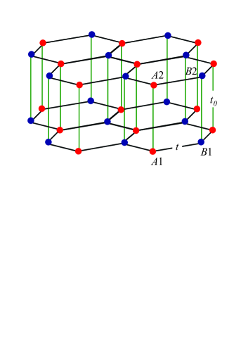
Figure 1: (Color online) Crystal structure of the AA-stacked bilayer graphene. The circles denote carbon atoms in the ${\cal A}$ (red) and ${\cal B}$ (blue) sublattices in the bottom (1) and top (2) layers. The unit cell of the AA-BLG consists of four atoms $A1$, $A2$, $B1$, and $B2$. Hopping integrals $t$ and $t_{0}$ correspond to the in-plane and inter-plane nearest-neighbor hopping.

II Tight-binding Hamiltonian

The crystal structure of the AA-BLG is shown in Fig. 1. The AA-BLG consists of two graphene layers, $1$ and $2$. Each carbon atom of the upper layer is located above the corresponding atom of the lower layer. Each layer consists of two triangular sublattices ${\cal A}$ and ${\cal B}$. The elementary unit cell of the AA-BLG contains four carbon atoms $A1$, $A2$, $B1$, and $B2$.

We write the single-particle Hamiltonian of the AA-BLG in the form

$$H_{0} = -t\sum_{\langle\mathbf{nm}\rangle i\sigma}\left(d^{{\dagger}}_{\mathbf{n}i{\cal A}\sigma}d^{\phantom{{\dagger}}}_{\mathbf{m}i{\cal B}\sigma}+H.c.\right)-$$

$$t_{0}\sum_{\mathbf{n}a\sigma}\left(d^{{\dagger}}_{\mathbf{n}1a\sigma}d^{\phantom{{\dagger}}}_{\mathbf{n}2a\sigma}+H.c.\right)-\mu\sum_{\mathbf{n}ia\sigma}d^{{\dagger}}_{\mathbf{n}ia\sigma}d^{\phantom{{\dagger}}}_{\mathbf{n}ia\sigma}\,.$$

Here $d^{{\dagger}}_{\mathbf{n}ia\sigma}$ and $d^{\phantom{{\dagger}}}_{\mathbf{n}ia\sigma}$ are the creation and annihilation operators of an electron with spin projection $\sigma$ in the layer $i=1,\,2$ on the sublattice $a={\cal A},{\cal B}$ at the position $\mathbf{n}$, $\mu$ is the chemical potential, and $\langle...\rangle$ denotes nearest-neighbor pair. The amplitude $t$ ($t_{0}$) in Eq. (II) describes the in-plane (inter-plane) nearest-neighbor hopping. For calculations, we will use the values of the hopping integrals $t\approx 2.57$ eV, $t_{0}\approx 0.36$ eV computed by DFT for multilayer AA systems in Ref. Charlier et al., 1992.

If we perform the unitary transformation

$$h^{\phantom{{\dagger}}}_{\mathbf{n}a\sigma}=\frac{d^{\phantom{{\dagger}}}_{\mathbf{n}1a\sigma}+d^{\phantom{{\dagger}}}_{\mathbf{n}2a\sigma}}{\sqrt{2}}\,,\;\;g^{\phantom{{\dagger}}}_{\mathbf{n}a\sigma}=\frac{d^{\phantom{{\dagger}}}_{\mathbf{n}1a\sigma}-d^{\phantom{{\dagger}}}_{\mathbf{n}2a\sigma}}{\sqrt{2}}\,,$$ (2)

then, Eq. (II) can be rewritten as

$$\!\!\!H_{0}\!=\!-t\!\!\!\sum_{\langle\mathbf{nm}\rangle\sigma}\!\!\!\left(h^{{\dagger}}_{\mathbf{n}{\cal A}\sigma}h^{\phantom{{\dagger}}}_{\mathbf{m}{\cal B}\sigma}+H.c.\right)-(\mu+t_{0})\!\!\sum_{\mathbf{n}a\sigma}h^{{\dagger}}_{\mathbf{n}a\sigma}h^{\phantom{{\dagger}}}_{\mathbf{n}a\sigma}$$

$$\!\!\!-t\!\!\sum_{\langle\mathbf{nm}\rangle\sigma}\!\!\!\left(g^{{\dagger}}_{\mathbf{n}{\cal A}\sigma}g^{\phantom{{\dagger}}}_{\mathbf{m}{\cal B}\sigma}+H.c.\right)-(\mu-t_{0})\!\!\sum_{\mathbf{n}a\sigma}g^{{\dagger}}_{\mathbf{n}a\sigma}g^{\phantom{{\dagger}}}_{\mathbf{n}a\sigma}\,.$$ (3)

Therefore, in this representation the Hamiltonian $H_{0}$ is a sum of two single-layered graphene Hamiltonians Castro Neto et al. (2009), with different effective chemical potential $\mu\pm t_{0}$.

The Hamiltonian (II) can be readily diagonalized. To perform the diagonalization, we switch to the fermion operators $h^{\phantom{{\dagger}}}_{\mathbf{k}a\sigma}$ and $g^{\phantom{{\dagger}}}_{\mathbf{k}a\sigma}$, which are defined in the momentum representation, and make the unitary transformation

$$\gamma^{\phantom{{\dagger}}}_{\mathbf{k}1\sigma}=\frac{h^{\phantom{{\dagger}}}_{\mathbf{k}\cal{A}\sigma}+h^{\phantom{{\dagger}}}_{\mathbf{k}\cal{B}\sigma}e^{i\varphi_{\mathbf{k}}}}{\sqrt{2}}\,,\;\gamma^{\phantom{{\dagger}}}_{\mathbf{k}2\sigma}=\frac{h^{\phantom{{\dagger}}}_{\mathbf{k}\cal{A}\sigma}-h^{\phantom{{\dagger}}}_{\mathbf{k}\cal{B}\sigma}e^{i\varphi_{\mathbf{k}}}}{\sqrt{2}}\,,$$

$$\gamma^{\phantom{{\dagger}}}_{\mathbf{k}3\sigma}=\frac{g^{\phantom{{\dagger}}}_{\mathbf{k}\cal{A}\sigma}+g^{\phantom{{\dagger}}}_{\mathbf{k}\cal{B}\sigma}e^{i\varphi_{\mathbf{k}}}}{\sqrt{2}}\,,\;\gamma^{\phantom{{\dagger}}}_{\mathbf{k}4\sigma}=\frac{g^{\phantom{{\dagger}}}_{\mathbf{k}\cal{A}\sigma}-g^{\phantom{{\dagger}}}_{\mathbf{k}\cal{B}\sigma}e^{i\varphi_{\mathbf{k}}}}{\sqrt{2}}\,,$$ (4)

where $\varphi_{\mathbf{k}}=\arg\left(f_{\mathbf{k}}\right)$,

$$f_{\mathbf{k}}=1+2\exp\!\left(\frac{3ik_{x}a_{0}}{2}\right)\!\cos\!\left(\!\!\frac{\sqrt{3}k_{y}a_{0}}{2}\!\!\right)\,,$$ (5)

and $a_{0}$ is the in-plane carbon-carbon distance. As a result, Hamiltonian (II) becomes

$$H_{0}=\!\sum_{\mathbf{k}s\sigma}\!\left(\varepsilon^{(s)}_{0\mathbf{k}}-\mu\right)\gamma^{{\dagger}}_{\mathbf{k}s\sigma}\gamma^{\phantom{{\dagger}}}_{\mathbf{k}s\sigma}\,.$$ (6)

In this equation, the band index $s$ runs from 1 to 4, and the band spectra $\varepsilon^{(s)}_{0\mathbf{k}}$ are

$$\varepsilon^{(1)}_{0\mathbf{k}}=-t_{0}-t\zeta_{\bf k}\,,\qquad\varepsilon^{(2)}_{0\mathbf{k}}=-t_{0}+t\zeta_{\bf k}\,,$$

$$\varepsilon^{(3)}_{0\mathbf{k}}=+t_{0}-t\zeta_{\bf k}\,,\qquad\varepsilon^{(4)}_{0\mathbf{k}}=+t_{0}+t\zeta_{\bf k}\,,$$ (7)

where $\zeta_{\bf k}=|f_{\bf k}|$. The band structure obtained is shown in Fig. 2. The bands $s=2$ and $s=3$ cross the Fermi level near the Dirac points $\mathbf{K}=2\pi(\sqrt{3},\,1)/(3\sqrt{3}a_{0})$ and $\mathbf{K}^{\prime}=2\pi(\sqrt{3},\,-1)/(3\sqrt{3}a_{0})$ [see Fig. 2(b)].

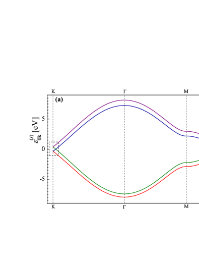
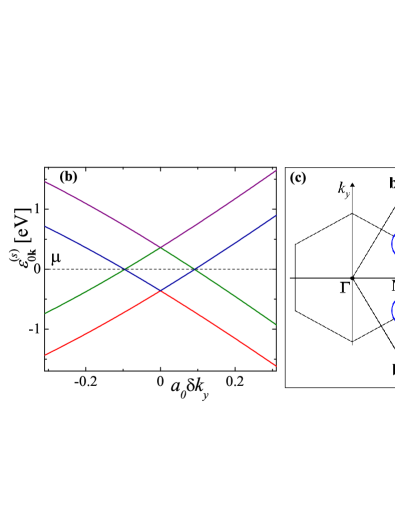
Figure 2: (Color online) (a) The single-particle band structure of the AA-stacked bilayer graphene. It consists of two single-layered graphene spectra shifted relative to each other by the energy $2t_{0}$. (b) The $\mathbf{k}$-dependence of the spectra $\varepsilon^{(s)}_{0\mathbf{k}}$ near the Dirac point ${\cal K}$ located at momentum $\mathbf{K}$. Here, $\mathbf{k}=\mathbf{K}+\delta k_{y}\mathbf{e}_{y}$. The intersection of the bands $s=2$ and $s=3$ occurs exactly at zero energy, which corresponds to the Fermi level of the undoped system. (c) The first Brillouin zone (hexagon) and the reciprocal lattice unit cell (rhombus) of the AA-BLG. The circles around ${\bf K}$ and ${\bf K}^{\prime}$ points correspond to Fermi surfaces of the doped system.

For undoped systems ($\mu=0$, half-filling) the Fermi surfaces are given by the equation $|f_{\bf k}|=t_{0}/t$. Since $t_{0}/t\ll 1$, we can expand the function $|f_{\bf k}|$ near the Dirac points and find that the Fermi surface consists of two circles with radius $k_{r}=2t_{0}/(3ta_{0})$. These Fermi surfaces transform into four circles in doped AA-BLG [see Fig. 2(c)].

The most important feature of this tight-binding band structure is that at half-filling the Fermi surfaces of both bands coincide. That is, the electron and hole components of the Fermi surface are perfectly nested. This property of the Fermi surfaces is quite stable against changes in the tight-binding Hamiltonian. It survives even if longer-range hoppings are taken into account, or a system with two non-equivalent layers is considered (e.g., similar to the single-side hydrogenated graphene sshg ). However, the electron interactions can destabilize such a degenerate spectrum, generating a gap our_preprint .

III Commensurate antiferromagnetic state

The single-electron spectrum described in the previous section changes qualitatively when interaction is included. Specifically, using mean field theory, we will demonstrate that the degenerate Fermi surface of the undoped AA-BLG is unstable with respect to the spontaneous generation of AFM order.

III.1 Mean-field equations

We approximate the electron-electron interaction by the Hubbard-like interaction Hamiltonian:

$$H_{\text{int}}=\frac{U}{2}\sum_{\mathbf{n}ia\sigma}\left(n_{\mathbf{n}ia\sigma}-\frac{1}{2}\right)\left(n_{\mathbf{n}ia\bar{\sigma}}-\frac{1}{2}\right)\,,$$ (8)

where $n_{\mathbf{n}ia\sigma}=d^{{\dagger}}_{\mathbf{n}ia\sigma}d^{\phantom{{\dagger}}}_{\mathbf{n}ia\sigma}$, and $\bar{\sigma}=-\sigma$. It is known that the on-site Coulomb interaction $U$ in graphene and other carbon systems is rather strong, but the estimates available in the literature vary considerably Ut ; U69 , ranging from 4-5 to 9-10 eV.

We analyze the properties of the Hamiltonian $H=H_{0}+H_{\text{int}}$ in the mean-field approximation. We choose the $x$-axis as the spin quantization axis, and write the order parameters as

$$\Delta_{ia}\equiv U\left\langle d^{{\dagger}}_{\mathbf{n}ia\uparrow}d^{\phantom{{\dagger}}}_{\mathbf{n}ia\downarrow}\right\rangle\,,$$ (9)

$$\Delta_{1\cal{A}}=\Delta_{2\cal{B}}=-\Delta_{1\cal{B}}=-\Delta_{2\cal{A}}\equiv\Delta\,,$$ (10)

and $\Delta$ is real. Such AFM order, when spin at any given site is antiparallel to spins at all four nearest-neighbor sites, is called in the literature G-type AFM. Other types of spin order are either unstable or metastable.

In the mean-field approximation, the interaction Hamiltonian has the form

$$H^{\rm MF}_{\text{int}} = {\cal N}\left[\frac{4\Delta^{2}}{U}-U(n^{2}-1)\right]+\frac{Ux}{2}\sum_{\mathbf{n}ia\sigma}n_{\mathbf{n}ia\sigma}$$ (11)

$$- \sum_{\mathbf{n}ia}\Delta_{ia}\left(d^{{\dagger}}_{\mathbf{n}ia\uparrow}d^{\phantom{{\dagger}}}_{\mathbf{n}ia\downarrow}+d^{{\dagger}}_{\mathbf{n}ia\downarrow}d^{\phantom{{\dagger}}}_{\mathbf{n}ia\uparrow}\right)\,,$$

where $x=n-1$ is the doping level, $n$ is the number of electrons per site, and ${\cal N}$ is the number of unit cells in the sample (a unit cell of AA-BLG consists of four carbon atoms, see Fig. 1). Below, when quoting numerical estimates for doping, we will write $x$ as a percentage of the total number of carbon atoms in the sample.

We introduce the four-component spinor

$$\psi^{{\dagger}}_{\mathbf{k}\sigma}=(d^{{\dagger}}_{\mathbf{k}1\cal{A}\sigma},d^{{\dagger}}_{\mathbf{k}2\cal{A}\sigma},d^{{\dagger}}_{\mathbf{k}1\cal{B}\sigma},d^{{\dagger}}_{\mathbf{k}2\cal{B}\sigma}),$$ (12)

which can be used to build an eight-component spinor $\Psi^{{\dagger}}_{\mathbf{k}}=(\psi^{{\dagger}}_{\mathbf{k}\uparrow},\psi^{{\dagger}}_{\mathbf{k}\downarrow}).$ In terms of this spinor, the mean field Hamiltonian $H^{\rm MF}=H_{0}+H^{\rm MF}_{\text{int}}$ can be written as

$$H^{\rm MF}={\cal N}E_{0}+\sum_{\mathbf{k}}\Psi^{{\dagger}}_{\mathbf{k}}\left(\begin{matrix}\hat{H}_{0\mathbf{k}}-\mu^{\prime}&\hat{\Delta}&\cr\hat{\Delta}&\hat{H}_{0\mathbf{k}}-\mu^{\prime}\cr\end{matrix}\!\!\!\right)\Psi^{\phantom{{\dagger}}}_{\mathbf{k}}\,,$$ (13)

where

$$E_{0}=\frac{4\Delta^{2}}{U}-U(n^{2}-1),\ \ \mu^{\prime}=\mu-\frac{Ux}{2}.$$ (14)

In these equations, $E_{0}$ is a $c$-number, $\mu^{\prime}$ is the renormalized chemical potential, $\hat{H}_{0\mathbf{k}}$, and $\hat{\Delta}$ are $4\times 4$ matrices

$$\hat{H}_{0\mathbf{k}}=-\left(\begin{matrix}0&t_{0}&tf_{\bf k}&0\cr t_{0}&0&0&tf_{\bf k}\cr tf_{\bf k}^{*}&0&0&t_{0}\cr 0&tf_{\bf k}^{*}&t_{0}&0\cr\end{matrix}\right)\,,$$ (15)

$$\hat{\Delta}=\left(\begin{matrix}-\Delta&0&0&0\cr 0&\Delta&0&0\cr 0&0&\Delta&0\cr 0&0&0&-\Delta\cr\end{matrix}\right)\,.$$ (16)

We diagonalize the $8\times 8$ matrix in Eq. (13) and obtain four doubly-degenerate bands

$$\varepsilon^{(1,4)}_{\mathbf{k}}=\mp\sqrt{\Delta^{2}+\left(t\zeta_{\mathbf{k}}+t_{0}\right)^{2}}\,,$$

$$\varepsilon^{(2,3)}_{\mathbf{k}}=\mp\sqrt{\Delta^{2}+\left(t\zeta_{\mathbf{k}}-t_{0}\right)^{2}}\,.$$ (17)

To determine the AFM gap $\Delta$ we should minimize the grand potential $\Omega$. The grand potential per unit cell is

$$\Omega=E_{0}-2T\!\sum_{s=1}^{4}\!\int\!\frac{d\mathbf{k}}{V_{\text{BZ}}}\ln\left[1+e^{(\mu^{\prime}-\varepsilon^{(s)}_{\mathbf{k}})/T}\right]\,,$$ (18)

where $V_{\text{BZ}}$ is the volume of the first Brillouin zone.

To evaluate integrals over the Brillouin zone it is convenient to introduce the density of states

$$\rho_{0}(\zeta)=\!\int\!\frac{d\mathbf{k}}{V_{\text{BZ}}}\delta(\zeta-\zeta_{\mathbf{k}})\,.$$ (19)

This function is non-zero only for $0<\zeta<3$. It is related to the graphene density of states $\rho_{\text{gr}}(E)$ as $\rho_{\text{gr}}(E)=\rho_{0}(|E/t|)/t$ (see Ref. Castro Neto et al., 2009).

Minimization of $\Omega$ with respect to $\Delta$ gives the equation

$$1 = \frac{U}{4t}\!\int\limits_{0}^{3}\!\!d\zeta\,\rho_{0}(\zeta)\!\!\left[F\left(\sqrt{\delta^{2}+(\zeta+\zeta_{0})^{2}}\right)\right.+$$ (20)

$$\left.F\left(\sqrt{\delta^{2}+(\zeta-\zeta_{0})^{2}}\right)\right]\,,$$

where $\delta=\Delta/t$, $\zeta_{0}=t_{0}/t$, and

$$F(\varepsilon)=\frac{f(-t\varepsilon-\mu^{\prime})-f(t\varepsilon-\mu^{\prime})}{\varepsilon},\;\;f(E)=\frac{1}{e^{\frac{\scriptstyle E}{\scriptstyle T}}+1}\,.$$ (21)

Equation (20) determines the gap $\Delta$ as a function of the renormalized chemical potential $\mu^{\prime}$. To find $\Delta$ as a function of doping, we need to relate the doping and the chemical potential. It is easy to prove that

$$n=1+x=-\frac{1}{4}\frac{\partial(\Omega-E_{0})}{\partial\mu^{\prime}}.$$ (22)

Then, using Eqs. (18) and (19) we derive

$$x=\frac{1}{2}\!\int\limits_{0}^{3}\!\!d\zeta\,\rho_{0}(\zeta)\!\!\left[G\left(\sqrt{\delta^{2}+(\zeta+\zeta_{0})^{2}}\right)\right.+$$

$$\left.G\left(\sqrt{\delta^{2}+(\zeta-\zeta_{0})^{2}}\right)\right]\,,$$ (23)

$${\rm where\ \ }G(\varepsilon)=f(-t\varepsilon-\mu^{\prime})+f(t\varepsilon-\mu^{\prime})-1\,.$$ (24)

Solving Eqs. (20) and (III.1) we obtain the AFM gap $\Delta(x,T)$ and the chemical potential $\mu(x,T)$.

The solutions of Eqs. (20) and (III.1) satisfy the following relations: $\Delta(-x,T)=\Delta(x,T)$ and $\mu(-x,T)=-\mu(x,T)$. They are consequences of the particle-hole symmetry of the model Hamiltonian. The next-nearest-neighbor hopping breaks this symmetry. However, our analysis shows that corrections, introduced by these terms, do not exceed 1–2% for the range of parameters characteristic of graphene systems. Assuming particle-hole symmetry, below we only consider electron doping, $x>0$.

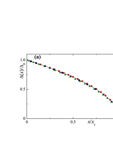
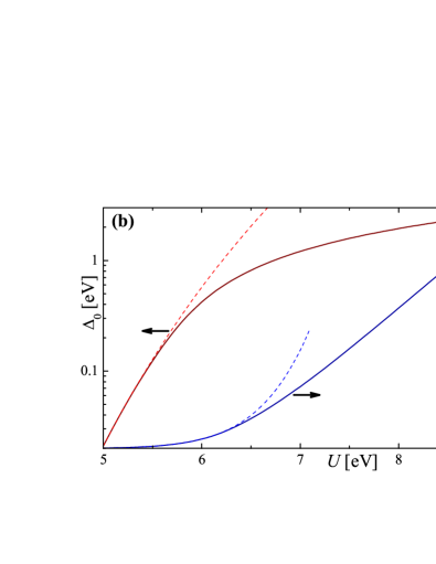
Figure 3: (Color online) (a) The AFM gap ratio $\Delta/\Delta_{0}$ versus doping $x/x_{c}$ for different values of the on-site Coulomb repulsion $U$: (red) squares correspond to $U=5.5$ eV, (blue) circles to $U=7$ eV, (green) triangles to $U=9$ eV. The solid (black) curve is $\Delta(x)/\Delta_{0}=\sqrt{1-x/x_{c}}$. (b) The dependencies $\Delta(x=0,T=0)\equiv\Delta_{0}$ and critical doping $x_{c}$ versus $U$. The solid curves are numerical solutions of Eqs. (25) and (26), while the dashed curves are calculated using the approximate analytical solution, Eqs. (29) and (30).

III.2 Zero temperature

If $T=0$, Eqs. (20) and (III.1) become

$$1 = \frac{U}{4t}\int\limits_{0}^{3}\!\!d\zeta\,\rho_{0}(\zeta)\!\!\left[\frac{1-\Theta\left(\displaystyle\mu^{\prime}/t-\sqrt{\delta^{2}+\left(\zeta+\zeta_{0}\right)^{2}}\right)}{\sqrt{\delta^{2}+\left(\zeta+\zeta_{0}\right)^{2}}}\right.+$$ (25)

$$\left.\frac{1-\Theta\left(\displaystyle\mu^{\prime}/t-\sqrt{\delta^{2}+\left(\zeta-\zeta_{0}\right)^{2}}\right)}{\sqrt{\delta^{2}+\left(\zeta-\zeta_{0}\right)^{2}}}\right]\,,$$

$$x = \frac{1}{2}\int\limits_{0}^{3}\!\!d\zeta\,\rho_{0}(\zeta)\!\!\left[\Theta\left(\displaystyle\mu^{\prime}/t-\sqrt{\delta^{2}+\left(\zeta+\zeta_{0}\right)^{2}}\right)\right.+$$ (26)

$$\left.\Theta\left(\displaystyle\mu^{\prime}/t-\sqrt{\delta^{2}+\left(\zeta-\zeta_{0}\right)^{2}}\right)\right]\,,$$

where $\Theta(x)$ is the step function. At half-filling, $n=1$, $x=0$, and $\mu=\mu^{\prime}=0$. The lower two bands are filled, the upper two bands are empty, and both $\Theta$-functions in Eq. (25) are zero for any $\zeta$.

When doping is introduced, analysis of the latter equations shows that $\mu^{\prime}$ changes abruptly from zero to the value $\mu^{\prime}>\Delta$. The gap $\Delta(x,T=0)$ decreases monotonously from $\Delta(x=0,T=0)\equiv\Delta_{0}$ to $0$, when $x$ increases from $0$ to some critical doping $x_{c}$. To find $x_{c}$ we must put $\delta=0$ into Eqs. (25) and (26) and solve them for $\mu^{\prime}$ and $x=x_{c}$.

Equations (25) and (26) can be solved analytically, if $\Delta_{0}\ll t,t_{0}$. Using the asymptotic expansions of integrals in these equations for small $\delta$ we obtain our_preprint2

$$\Delta(x,0) = \Delta_{0}\sqrt{1\!-\frac{x}{x_{c}}}\,,$$ (27)

$$\mu(x,0) = \Delta_{0}\left[{\rm sgn\,}(x)-\frac{x}{2x_{c}}\right]+\frac{Ux}{2}\,,$$ (28)

$$x_{c} = \frac{\Delta_{0}\rho_{0}(\zeta_{0})}{2t}\cong\frac{\Delta_{0}t_{0}}{\pi\sqrt{3}t^{2}}\;\;{\rm\ when\ }t_{0}\ll t\,.$$ (29)

In this limit the value of $\Delta_{0}$ is given by the relation our_preprint

$$\Delta_{0}=2\sqrt{t_{0}(3t-t_{0})}\exp\left\{-\frac{4t-U\eta(\zeta_{0})}{2U\rho_{0}(\zeta_{0})}\right\}\,,$$ (30)

where

$$\eta(\zeta_{0})\!=\!\int\limits_{0}^{3}\!\!d\zeta\left[\frac{\rho_{0}(\zeta)}{\zeta+\zeta_{0}}+\frac{\rho_{0}(\zeta)-\rho_{0}(\zeta_{0})}{\left|\zeta-\zeta_{0}\right|}\right].\;\;\$$ (31)

The dependence of the ratio $\Delta(x,0)/\Delta_{0}$ on $x/x_{c}$ for different values of $U$ is shown in Fig. 3(a). Figure 3(b) shows $\Delta_{0}$ and $x_{c}$ as functions of $U$ calculated both numerically [Eqs. (25) and (26)] and analytically [Eqs. (29) and (30)]. Equations (28), (29) together with Eq. (30) for $\Delta_{0}$ are valid if $U\lesssim 6$ eV. However, Eq. (27) is accurate for any $U$, provided that $x_{c}$ and $\Delta_{0}$ are calculated numerically from Eqs. (25) and (26) [see Fig. 3(a)].

III.3 Finite temperatures

In this subsection we will analyze the finite-temperature solutions of the mean field equations (20) and (III.1). However, it is necessary to remember that in 2D systems no long-range order is possible if $T>0$. In such a situation the mean field solutions characterize the short-range order, which survives for sufficiently low $T$. The effects beyond the mean field approximation will be discussed in subsection III.4.

Solving numerically the mean field equations (20) and (III.1), we find $\Delta$ as a function of doping $x$ and temperature $T$ (see Fig. 4). The temperature $T_{\rm MF}$ at which $\Delta$ vanishes is the mean field transition temperature (see inset of Fig. 4). The transition temperature, as a function of doping $x$, is not a single-valued function. Instead, it demonstrates a pronounced re-entrant behavior. We discuss this unusual phenomenon in more details in Sections IV, V, and VI.

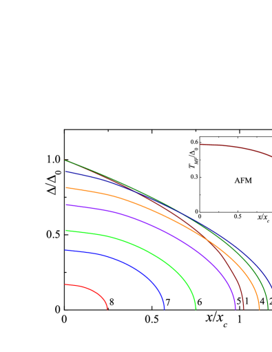
Figure 4: (Color online) The dependence of $\Delta(x,T)$ on doping $x$ calculated for $U=5.5$ eV and different $T/\Delta_{0}$: (1) $T/\Delta_{0}=0.06$, (2) $T/\Delta_{0}=0.17$, (3) $T/\Delta_{0}=0.33$, (4) $T/\Delta_{0}=0.41$, (5) $T/\Delta_{0}=0.47$, (6) $T/\Delta_{0}=0.52$, (7) $T/\Delta_{0}=0.55$, and (8) $T/\Delta_{0}=0.58$. Inset: The dependence of the mean-field transition temperature on doping. The re-entrance from PM to AFM state exists in the doping range $x_{c}<x<1.231x_{c}$; $x_{c}=0.128$% and $\Delta_{0}=0.124$ eV.

Equations (20) and (III.1) can be simplified in the case of small gap, when $\Delta_{0}\ll t_{0},t$. Neglecting terms of the order of $\Delta_{0}^{2}/t^{2}$ in Eq. (20) and taking into account Eq. (30) for $\Delta_{0}$, we obtain the following equation for $\Delta$

$$\ln\frac{\Delta_{0}}{\Delta} = \frac{1}{4}\!\!\int\limits_{\Delta/T}^{\infty}\!\!dz\operatorname{acosh}\left(\frac{zT}{\Delta}\right)$$

$$\times \!\!\left[{\cosh^{-2}\left(\displaystyle\frac{z-\mu^{\prime}/T}{2}\right)}+{\cosh^{-2}\left(\displaystyle\frac{z+\mu^{\prime}/T}{2}\right)}\right].$$

In the same limit, we derive from Eq. (III.1) the relation between $\mu^{\prime}$ and $x$ in the form

$$\frac{x}{x_{c}}=\frac{T}{2\Delta_{0}}\!\!\!\int\limits_{\Delta/T}^{\infty}\!dz\sqrt{z^{2}-\frac{\Delta^{2}}{T^{2}}}\!$$

$$\times\left[{\cosh^{-2}\left(\displaystyle\frac{z-\mu^{\prime}/T}{2}\right)}-{\cosh^{-2}\left(\displaystyle\frac{z+\mu^{\prime}/T}{2}\right)}\right]\,.$$

At half-filling ($x=0$) we find from Eq. (III.3) the BCS-like result $T_{\rm MF}(0)\cong 0.567\Delta_{0}$. If we normalize $x$ by $x_{c}$ and $\Delta$, $\mu^{\prime}$ and $T$ by $\Delta_{0}$, then, Eqs. (III.3) and (III.3) do not include any parameter characterizing the AA-BLG band structure. Thus, if the electron interaction $U$ is not large, the obtained results do not depend on details specific to the AA-BLG and are valid for other systems with imperfect nesting RiceMod ; our_Rice_model ; our_pnic .

III.4 Crossover temperature

In 2D systems, finite-temperature fluctuations destroy the AFM long-range order. Then, the results obtained above in the mean-field approximation are valid only if the mean-field correlation length $\xi=v_{\rm F}/\Delta$ is smaller than the spin-wave correlation length $\xi_{sw}$ (here $v_{\rm F}\cong 3a_{0}t/2$ is the Fermi velocity in our model). Otherwise, short-range ordering of spins disappears, and we cannot define the AFM order even locally.

In the limit $\xi_{\rm sw}>\xi$, the spin fluctuations can be described using the nonlinear $\sigma$-model with Lagrangian chak ; Manousakis

$${\cal L}_{\rm sw}=\frac{\rho}{2}\left[(\partial_{t}{\bf D})^{2}-c_{\rm sw}^{2}(\partial_{\bf r}{\bf D})^{2}\right],$$ (34)

where ${\bf D}$ is the unit vector along the local AFM magnetization. The spin-wave stiffness $\rho$ and velocity $c_{\rm sw}$ can be evaluated from Eqs. (7.89) and (7.90) of Ref. schakel,

$$c_{\rm sw}=\frac{v_{\rm F}}{\sqrt{2}},\quad\rho=\begin{cases}t_{0}/(8\pi v_{\rm F}^{2}),&\text{if $t_{0}\gg\Delta$},\\ \Delta/(16\pi v_{\rm F}^{2}),&\text{if $t_{0}\ll\Delta$}.\end{cases}$$ (35)

The correlation function $K(\mathbf{r})=\langle\mathbf{D}(\mathbf{r})\mathbf{D}(0)\rangle$ can be obtained using the Lagrangian (34). At large distances it behaves as chak ; Manousakis

$$K(\mathbf{r})\approx 1-\frac{T}{\pi\rho v_{\rm F}^{2}}\ln\left(\frac{e^{\gamma}\sqrt{2}\,rT}{3a_{0}t}\right)\,,$$ (36)

where $\gamma$ is the Euler’s constant. The spin-wave correlation length $\xi_{\rm sw}$ describing the characteristic size of the short-range AFM order can be estimated using the equation $K(\xi_{\rm sw})=0$. Thus, we have

$$\xi_{\rm sw}\approx\frac{a_{0}t}{T}\exp\left(\frac{2\pi\rho c_{\rm sw}^{2}}{T}\right)\,.$$ (37)

Solving the equation $\xi_{\rm sw}=\xi$, we find the crossover temperature $T^{*}$ between the short-range AFM and the PM. The short-range AFM order exists over distances of about $\xi_{\rm sw}\gg a_{0}$, if $T<T^{*}$, and it is destroyed if $T>T^{*}$. Our numerical analysis shows that $T^{*}(x)/T_{\rm MF}(x)\approx 0.8$ - $0.9$ for any ratio $\Delta/t$. Thus, the mean-field transition temperature gives an appropriate estimate for the AFM-to-PM crossover temperature.

IV Incommensurate antiferromagnetic state

The G-type AFM state considered above has the smallest value of the grand thermodynamic potential $\Omega$ among other states with commensurate magnetic order. However, further optimization of $\Omega$ could be achieved if we allow the local direction of the AFM magnetization slightly rotate from site to site RiceMod . Then, the translation invariance with a lattice period disappears. Such a state is referred to as incommensurate (or helical) AFM. The complex order parameter for this state has a form

$$\Delta_{\mathbf{n}ia}=U\left\langle d^{{\dagger}}_{\mathbf{n}ia\uparrow}d^{\phantom{{\dagger}}}_{\mathbf{n}ia\downarrow}\right\rangle=e^{i\mathbf{qn}}\Delta_{ia}\,,$$ (38)

where $\mathbf{q}$ describes the spatial variation of the AFM magnetization direction, the position vector $\mathbf{n}$ specifies the location of a given carbon atom, and $\Delta_{ia}$ satisfies Eqs. (10). The averaged electron spin $\mathbf{S}_{\mathbf{n}ia}$ at site $\mathbf{n}$ lies in the $xy$-plane. It is related to the order parameter as $\langle d^{{\dagger}}_{\mathbf{n}ia\uparrow}d^{\phantom{{\dagger}}}_{\mathbf{n}ia\downarrow}\rangle=S^{x}_{\mathbf{n}ia}+iS^{y}_{\mathbf{n}ia}$. As a result, we obtain

$$\mathbf{S}_{\mathbf{n}ia}=\frac{\Delta_{ia}}{U}\left(\cos(\mathbf{qn}),\,\sin(\mathbf{qn})\right)\,.$$ (39)

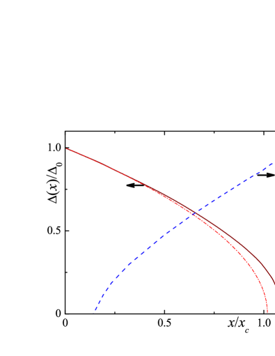
Figure 5: (Color online) The dependence of $\Delta$ (red solid curve) and $|\mathbf{q}|$ (blue dashed curve) on doping $x$ calculated for $T/\Delta_{0}=0.06$. The dot-dashed curve is the gap $\Delta$ calculated for $\mathbf{q}=0$ and $U=8$ eV. The doping $x$ is normalized by the critical doping $x_{c}$, calculated for the commensurate AFM state. The incommensurate AFM exists in a slightly larger doping range than the commensurate AFM. Note that the gap for commensurate AFM remains non-zero even for $x>x_{c}$. This is a manifestation of the re-entrance, see inset of Fig. 4.

The mean-field version of the interaction Hamiltonian (8) corresponding to the order parameter $\Delta_{\mathbf{n}ia}$, Eq. (38), can be written in the momentum representation as [c.f. Eq. (11)]

$$H_{\text{int}} \!\!=\!\! {\cal N}\!\left[\frac{4\Delta^{2}}{U}-U(n^{2}-1)\right]+\frac{Ux}{2}\!\sum_{\mathbf{k}ia\sigma}n_{\mathbf{k}ia\sigma}-$$

$$\!\!\sum_{\mathbf{k}ia}\Delta_{ia}\left(d^{{\dagger}}_{\mathbf{k}+\frac{\scriptstyle\mathbf{q}}{\scriptstyle 2}ia\uparrow}d^{\phantom{{\dagger}}}_{\mathbf{k}-\frac{\scriptstyle\mathbf{q}}{\scriptstyle 2}ia\downarrow}+d^{{\dagger}}_{\mathbf{k}-\frac{\scriptstyle\mathbf{q}}{\scriptstyle 2}ia\downarrow}d^{\phantom{{\dagger}}}_{\mathbf{k}+\frac{\scriptstyle\mathbf{q}}{\scriptstyle 2}ia\uparrow}\right)\,.$$

It is convenient to redefine the spinor $\Psi$ (see Sec. III.1):

$$\Psi^{{\dagger}}_{\mathbf{kq}}=(\psi^{{\dagger}}_{\mathbf{k}+\mathbf{q}/2\uparrow},\psi^{{\dagger}}_{\mathbf{k}-\mathbf{q}/2\downarrow}).$$ (41)

We can rewrite the mean-field Hamiltonian $H_{0}+H_{\rm int}^{\rm MF}$ in the form

$$H={\cal N}E_{0}+\!\sum_{\mathbf{k}}\Psi^{{\dagger}}_{\mathbf{kq}}\!\left(\begin{matrix}\hat{H}_{0\mathbf{k}+\frac{\scriptstyle\mathbf{q}}{\scriptstyle 2}}-\mu^{\prime}\!\!&\hat{\Delta}&\cr\hat{\Delta}&\!\!\hat{H}_{0\mathbf{k}-\frac{\scriptstyle\mathbf{q}}{\scriptstyle 2}}-\mu^{\prime}\cr\end{matrix}\!\!\!\right)\!\Psi^{\phantom{{\dagger}}}_{\mathbf{kq}},$$ (42)

where $\hat{H}_{0\mathbf{k}}$ and $\hat{\Delta}$ are given by Eqs. (15) and (16), respectively.

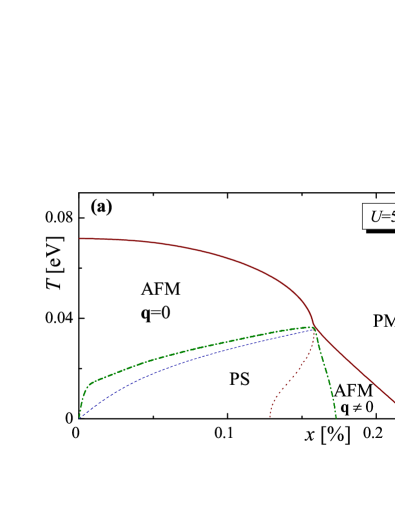
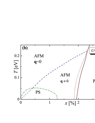
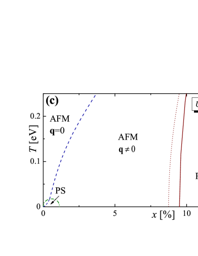
Figure 6: (Color online) The phase diagram of the model in the ($x,\,T$) plane, calculated for the electron doping $x>0$ and $U=5.5$ eV (a), $U=6.5$ eV (b), and $U=8$ eV (c). Solid (red) curves are $T_{\rm MF}(x)$, (blue) dashed curves are $T^{q}(x)$, at which the commensurate-incommensurate transition occurs. The dotted (red) curves are $T_{\rm MF}(x)$, calculated without taking into account the incommensurate AFM state. The dot-dashed (green) curves show the region of phase separation. For hole doping ($x<0$) the results are the same.

The electron spectrum in the incommensurate AFM state is found by diagonalization of the $8\times 8$ matrix in Eq. (42). It consists of $8$ non-degenerate bands, $E_{\mathbf{k},\mathbf{q}}^{(s)}$, $s=1,2,\dots,8$. The analytical expression for $E_{\mathbf{k},\mathbf{q}}^{(s)}$ can be obtained in the limit $|\mathbf{q}|\ll 1/a_{0}$,

$$\frac{E_{\mathbf{k},\mathbf{q}}^{(s)}}{t}\!\approx\!\pm\frac{\zeta_{\mathbf{k}+\frac{\scriptstyle\mathbf{q}}{\scriptstyle 2}}-\zeta_{\mathbf{k}-\frac{\scriptstyle\mathbf{q}}{\scriptstyle 2}}}{2}\!\pm\!\sqrt{\frac{\!\Delta^{2}}{t^{2}}+\!\!\left[\frac{t_{0}}{t}\pm\frac{\zeta_{\mathbf{k}+\frac{\scriptstyle\mathbf{q}}{\scriptstyle 2}}+\zeta_{\mathbf{k}-\frac{\scriptstyle\mathbf{q}}{\scriptstyle 2}}}{2}\right]^{2}}\!\!.$$ (43)

If $\mathbf{q}=0$, this spectrum coincides with the spectrum of Eqs. (III.1).

The expression for the grand potential $\Omega$ has similar structure as Eq. (18), but now the summation includes eight bands:

$$\Omega=E_{0}-T\sum_{s=1}^{8}\!\int\!\frac{d\mathbf{k}}{V_{\text{BZ}}}\ln\left[1+e^{(\mu^{\prime}-E^{(s)}_{\mathbf{k},\mathbf{q}})/T}\right].$$ (44)

Minimization of $\Omega$ with respect to $\Delta$ and $\mathbf{q}$, together with the condition relating $x$ and $\mu^{\prime}$ gives the closed system of equations for calculating $\Delta(x,T)$, $\mathbf{q}(x,T)$, and $\mu(x,T)$:

$$\frac{\partial\Omega}{\partial\Delta}=0\,,\;\;\frac{\partial\Omega}{\partial\mathbf{q}}=0\,,\;\;1+x=-\frac{\partial(\Omega-E_{0})}{\partial\mu^{\prime}}\,.$$ (45)

We calculate the functions $\Delta(x,T)$, $\mathbf{q}(x,T)$, and $\mu(x,T)$ numerically for different values of $U$. Typical curves $\Delta(x)$ and $|\mathbf{q}(x)|$ are shown in Fig. 5. For comparison, the curve $\Delta(x)$ calculated for the commensurate AFM is also plotted. We see that the incommensurate AFM state exists in a slightly wider doping range than the commensurate one. The incommensurate phase arises at arbitrary small doping if $T=0$. At non-zero $T$ the commensurate AFM state is stable until doping exceeds some $T$-dependent threshold $x^{q}(T)$. The curve $T^{q}(x)$ separates the incommensurate and commensurate AFM states; the more symmetrical AFM state with $\mathbf{q}=0$ lies above $T^{q}(x)$.

The phase diagrams of the model in the $x$–$T$ plane are shown in Fig. 6 for three different values of $U$. The diagrams for small $U$ ($\lesssim 6$ eV) and large $U$ ($\gtrsim 6$ eV) demonstrate a qualitative difference. Namely, for small $U$ [Fig. 6(a), $U=5.5$ eV] the re-entrance, seen in the inset of Fig. 4, disappears. It is masked by the incommensurate AFM phase. For larger $U$, however, it survives, Fig. 6(b,c). Re-entrance is an unusual phenomenon because the ordering occurs as the temperature increases. If re-entrance is a genuine feature of the model, or it is an artifact of the mean field approximation, whose reliability deteriorates when $U$ grows, we do not know. Similar behavior was predicted theoretically for quarter-filled Hubbard model at moderate interaction strength theory_reentrance , and numerically for classical rotor model rotor_reentrance1999 .

V Phase separation

In our discussion above we implicitly assumed that the ground state of the AA-BLG is spatially homogeneous. However, this is not always true: it was predicted in Ref. our_preprint2, that there is a finite doping range where the AA-BLG separates in two phases with unequal electron densities $n_{1,2}=1+x_{1,2}$. Indeed, if $\Delta_{0}\ll t,t_{0}$ we can use Eq. (28) and obtain that

$$\frac{\partial\mu}{\partial x}<0,{\rm\ \ if\ \ }\frac{U}{t}<\frac{\pi\sqrt{3}t}{t_{0}}.$$ (46)

The negative value of the derivative $\partial\mu/\partial x$ indicates the instability of the homogeneous state toward phase separation thermodyn .

If the possibility of the incommensurate AFM is ignored, then a zero-temperature phase separation our_preprint2 occurs between the AFM insulator ($x_{1}=0$) and the PM ($U\lesssim 6$ eV) or the AFM ($U\gtrsim 6$ eV) metal ($x_{2}>0$). Here we study phase separation taking into account the incommensurate AFM phase and non-zero temperature. We numerically analyze the stability of the homogeneous state using the dependence of the chemical potential $\mu$ on the doping $x$.

A typical dependence $\mu(x)$ for non-zero temperature is shown in Fig. 7. The derivative $\partial\mu/\partial x$ is negative in some range of doping and the system separates in commensurate ($\mathbf{q}=0$, $x_{1}<x$) and incommensurate ($\mathbf{q}\neq 0$, $x_{2}>x$) AFM phases. The doping concentrations $x_{1}$ and $x_{2}$ are found using the Maxwell construction thermodyn : the (black) horizontal line is drawn in such a manner that the areas of the shaded regions in Fig. 7 are equal to each other. When temperature increases, the doping range $x_{1}<x<x_{2}$, where the phase separation exists, becomes narrower and disappears at some critical temperature. Our calculations show that the separated phases are AFM with $\mathbf{q}=0$ and $\mathbf{q}\neq 0$ for any values of the model parameters. The region of the phase separation in the $(x,T)$-phase diagram is shown in Fig. 6 by (green) dot-dashed lines.

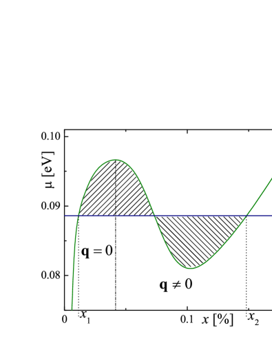
Figure 7: (Color online) Chemical potential $\mu$ of the homogeneous state versus doping $x$; $U=5.5$ eV and $T=0.014$ eV. The vertical dot-dashed line separates the AFM states with $\mathbf{q}=0$ and $\mathbf{q}\neq 0$. In the doping range $x_{1}<x<x_{2}$, phase separation occurs. The values $x_{1,2}$ are determined by the Maxwell construction: the horizontal (black) line is drawn in such a manner that the areas of the shaded regions are equal to each other.

VI Discussion

In this paper we study the evolution of the electron properties of AA-BLG with doping $x$ and temperature $T$. We calculate the phase diagram of the system in the $(x,T)$-plane. This diagram includes regions of the AFM commensurate and incommensurate states, a region of phase separation, and the PM state. With good accuracy, the electronic properties of the AA-BLG are symmetric with respect to the electron ($x>0$) or hole ($x<0$) doping. The maximum crossover temperature between the short-range AFM and the PM states depends on the on-site Coulomb repulsion $U$. For example, AFM ordering can exist up to temperatures of about 50 K if $U=5.5$ eV and to temperatures much higher than room temperature if $U\gtrsim 6.5$ eV. At present, there is no consensus on the value of the on-site Coulomb repulsion in graphene-based materials. However, it is commonly accepted that $U$ lies is in the range $6<U<10$ eV and, consequently, the AFM state can be observed in the AA-BLG.

The critical doping value $x_{c}$, at which the AFM is replaced by the PM, also strongly depends on $U$, changing from $\sim 0.1$ % if $U=5.5$ eV to $\sim 10$ % if $U=8$ eV. For graphene systems, doping of about $10\,\%$ and even higher was achieved CaK . Similar to single-layered graphene, the AA-BLG can be doped by using appropriate dopants CaK ; absor , choosing the substrate and applying a gate voltage Geim ; Kim , or by combinations of these methods.

We predict the existence of phase separation in the AA-BLG. The separated phases have different electron concentrations, $x_{1}$ and $x_{2}$, and the phase separation will be frustrated by long-range Coulomb repulsion Cul . In this case the formation of nano-scale inhomogeneities is more probable. The electron-rich phase (incommensurate AFM) is metal and the electron-poor phase (commensurate AFM insulator if $T=0$) is insulator or “bad” metal. Thus, the percolative insulator-metal transition will occur when the doping $x$ exceeds some threshold value our_preprint2 , which is about $0.5(x_{1}+x_{2})$ in 2D systems. Phase separation exists in the doping range $x_{1}<x<x_{2}$, and $x_{2}\lesssim 1$ % for any value of $U$. Depending on $U$, phase separation could be observed from 30-40 K to room and even higher temperatures (see Fig. 6). This makes AA-BLG promising for applications.

The incommensurate AFM phase is mathematically equivalent to the Fulde-Ferrel-Larkin-Ovchinnikov state in superconductors fflo ; sheehy2007 , which is sensitive to disorder Takada and difficult to observe experimentally. Consequently, it is reasonable to expect that the incommensurate AFM phase can be destroyed by factors our study did not account for. Our calculations predict that in this case the region of phase separation changes only slightly in the phase diagram. However, the separated phases would be the AFM insulator and PM ($U\lesssim 6$ eV) of AFM metal ($U\gtrsim 6$ eV).

To conclude, we studied the phase diagram of the AA-stacked graphene bilayers on the doping–temperature plane. It consists of paramagnetic and antiferromagnetic (both commensurate and incommensurate) homogeneous phases. In addition, a region of phase separation is also identified. Magnetic properties of the AA-BLG may survive even at room temperature.

References

- (1)
- Castro Neto et al. (2009) A.H. Castro Neto, F. Guinea, N.M.R. Peres, K.S. Novoselov, and A. K. Geim, Rev. Mod. Phys. 81, 109 (2009).
- Abergel et al. (2010) D.S.L. Abergel, V. Apalkov, J. Berashevich, K. Ziegler, and T. Chakraborty, Adv. Phys. 59, 261 (2010).
- Rozhkov et al. (2011) A.V. Rozhkov, G. Giavaras, Y.P. Bliokh, V. Freilikher, and F. Nori, Physics Reports 503, 77 (2011).
- McCann and Fal’ko (2006) E. McCann and V. I. Fal’ko, Phys. Rev. Lett. 96, 086805 (2006); E.V. Castro, N.M.R. Peres, T. Stauber, and N.A.P. Silva, ibid., 100, 186803 (2008); R. Nandkishore and L. Levitov, ibid. 104, 156803 (2010a); Phys. Rev. B 82, 115124 (2010b); F. Zhang, H. Min, M. Polini, and A.H. MacDonald, ibid., 81, 041402 (2010); Y. Lemonik, I.L. Aleiner, C. Toke, and V.I. Fal’ko, ibid., 82, 201408 (2010); O. Vafek and K. Yang, ibid., 81, 041401 (2010); J. Nilsson, A.H. Castro Neto, N.M.R. Peres, and F. Guinea, ibid., 73, 214418 (2006).
- Feldman et al. (2009) B.E. Feldman, J. Martin, and A. Yacoby, Nat. Phys. 5, 889 (2009).
- Mayorov et al. (2011) A.S. Mayorov D.C. Elias, M. Mucha-Kruczynski, R.V. Gorbachev, T. Tudorovskiy, A. Zhukov, S.V. Morozov, M.I. Katsnelson, V.I. Fal’ko, A.K. Geim, K.S. Novoselov, Science 333, 860 (2011).
- (8) J.-K. Lee, S.-Ch. Lee, J.-P. Ahn, S.-Ch. Kim, J.I.B. Wilson, and P. John, J. Chem. Phys. 129, 234709 (2008).
- Liu et al. (2009) Z. Liu, K. Suenaga, P. J. F. Harris, and S. Iijima, Phys. Rev. Lett. 102, 015501 (2009).
- Borysiuk et al. (2011) J. Borysiuk, J. Soltys, and J. Piechota, J. of Appl. Phys. 109, 093523 (2011).
- de Andres et al. (2008) P.L. de Andres, R. Ramírez, and J.A. Vergés, Phys. Rev. B 77, 045403 (2008).
- Prada et al. (2011) E. Prada, P. San-Jose, L. Brey, and H. Fertig, Solid State Commun. 151, 1075 (2011).
- Chiu et al. (2010) C.W. Chiu, S.H. Lee, S.C. Chen, F.L. Shyu, and M.F. Lin, New J. Phys. 12, 083060 (2010).
- Ho et al. (2010) Y.-H. Ho, J.-Y. Wu, R.-B. Chen, Y.-H. Chiu, and M.-F. Lin, Appl. Phys. Lett. 97, 101905 (2010).
- (15) S. Novoselov, E. McCann, S.V. Morozov, V.I. Fal’ko, M.I. Katsnelson, U. Zeitler, D. Jiang, F. Schedin, and A.K. Geim, Nat. Phys. 2, 177 (2006); S. Latil and L. Henrard, Phys. Rev. Lett. 97, 036803 (2006); B. Partoens and F.M. Peeters, Phys. Rev. B74, 075404 (2006); H. Min, B. Sahu, S.K. Banerjee, and A.H. MacDonald, Phys. Rev. B75, 155115 (2007).
- (16) A.L. Rakhmanov, A.V. Rozhkov, A.O. Sboychakov, and F. Nori, Phys. Rev. Lett. 109, 206801 (2012).
- (17) A.L. Rakhmanov, A.V. Rozhkov, A.O. Sboychakov, and F. Nori, Phys. Rev. B87, 121401(R) (2013).
- Charlier et al. (1992) J.-C. Charlier, J.-P. Michenaud, and X. Gonze, Phys. Rev. B 46, 4531 (1992).
- (19) H. Xiang, E.J. Kan, Su-Huai Wei, X.G. Gong, and M.-H. Whangbo, Phys. Rev. B 82, 165425 (2010); B. Pujari, S. Gusarov, M. Brett, and A. Kovalenko, Phys. Rev. B 84, 041402(R) (2011); L. Openov, A. Podlivaev, Semiconductors, 46, 199 (2012); L. Openov, A. Podlivaev, Physica E 44, 1894 (2012); L. Openov, A. Podlivaev, Technical Physics 57, 1603 (2012).
- (20) T.M. Rice, Phys. Rev. B2, 3619 (1970).
- (21) L. Pisani, J.A. Chan, B. Montanar, and N.M. Harrison, Phys. Rev. B75, 064418 (2007); D. Soriano, N. Leconte, P. Ordejón, J.-C. Charlier, J.-J. Palacios, and S. Roche, Phys. Rev. Lett. 107, 016602 (2011).
- (22) T.O. Wehling, E. Şaşogŭ, C. Friedrich, A.I. Lichtenstein, M.I. Katsnelson, and S. Blügel, Phys. Rev. Lett. 106, 236805 (2011); A. Du, Y.H. Ng, N.J. Bell, Z. Zhu, R. Amal, and S.C. Smith, J. Phys. Chem. Lett. 2, 894 (2011).
- (23) A.L. Rakhmanov, A.V. Rozhkov, A.O. Sboychakov, F. Nori, Phys. Rev. B 87, 075128 (2013).
- (24) A.O. Sboychakov, A.V. Rozhkov, K.I. Kugel, A.L. Rakhmanov, F. Nori, preprint arXiv:1304.2175 (unpublished).
- (25) S. Chakravarty, B.I. Halperin, and D.R. Nelson, Phys. Rev. B, 39, 2344 (1989).
- (26) E. Manousakis, Rev. Mod. Phys. 63, 1 (1991).
- (27) A.M.J. Schakel, Boulevard of Broken Symmetries: effective field theories of condensed matter (World Scientific, Singapore, 2008)
- (28) A. Kobayashi, Y. Tanaka, M. Ogata, and Y. Suzumura, J. Phys. Soc. Jpn. 73, 1115 (2004); J. Merino, A. Greco, N. Drichko, and M. Dressel, Phys. Rev. Lett. 96, 216402 (2006).
- (29) B. Hetényi, M.H. Müser, and B.J. Berne, Phys. Rev. Lett. 83, 4606 (1999).
- (30) M. Le Bellac, F. Mortessagne, and G.G. Batrouni, Equilibrium and Non-Equilibrium Statistical Thermodynamics, (Cambridge Univ. Press, Cambridge 2004).
- (31) J.L. McChesney, A. Bostwick, T. Ohta, T. Seyller, K. Horn, J. González, and E. Rotenberg, Phys. Rev. Lett. 104, 136803 (2010).
- (32) S.Y. Zhou, D.A. Siegel, A.V. Fedorov, and A. Lanzara, Phys. Rev. Lett. 101, 086402 (2008).
- (33) T.J. Echtermeyer, L. Britnell, P.K. Jasnos, A. Lombardo, R.V. Gorbachev, A.N. Grigorenko, A.K. Geim, A.C. Ferrari, and K.S. Novoselov, Nature Communs. 2, 458 (2011).
- (34) S. Kim, I. Jo, D.C. Dillen, D.A. Ferrer, B. Fallahazad, Z. Yao, S.K. Banerjee, and E. Tutuc, Phys. Rev. Lett. 108, 116404 (2012).
- (35) J. Lorenzana, C. Castellani, and C. Di Castro, Phys. Rev. B64, 235127, 235128 (2001); R. Jamei, S. Kivelson, and B. Spivak, Phys. Rev. Lett. 94, 056805 (2005); K.I. Kugel, A.L. Rakhmanov, and A.O. Sboychakov, Phys. Rev. Lett. 95, 267210 (2005).
- (36) P. Fulde and R.A. Ferrel, Phys. Rev. 135, A550 (1964); A.I. Larkin and Yu.N. Ovchinnikov, Sov. Phys. - JETP 20, 762 (1965); L.G. Aslamazov, ibid. 28, 773 (1969).
- (37) D.E. Sheehy, L. Radzihovsky, Ann. of Phys. 322, 1790 (2007).
- (38) S. Takada, Prog. Theor. Phys. 43, 27 (1970).