Primordial non-Gaussianity estimation using 21 cm tomography
from the epoch of reionization

Abstract

Measuring the small primordial nonGaussianity (PNG) predicted by cosmic inflation theories may help diagnose them. The detectability of PNG by its imprint on the 21 cm power spectrum from the epoch of reionization is reassessed here in terms of $f_{NL}$, the local nonlinearity parameter. We find that an optimum, multi-frequency observation by SKA can achieve $\Delta f_{NL}\sim 3$ (comparable to recent Planck CMB limits), while a cosmic-variance-limited array of this size like Omniscope can even detect $\Delta f_{NL}\sim 0.2$. This substantially revises the methods and results of previous work.

I Introduction

The theory of cosmic inflation Guth81 ; Linde82 , advanced to solve the cosmological horizon and flatness problems, also explains the initial fluctuations which later gave rise to galaxies and large-scale structure in the universe. While inflation generically predicts initial matter density fluctuations with an approximately Gaussian random distribution, the small deviations from Gaussianity that characterize different inflation models have been suggested to provide an observational probe to test and distinguish the models. While purely Gaussian initial density fluctuations are fully described by their power spectrum, primordial non-Gaussianity (PNG) requires higher-order statistics to characterize it, the lowest-order being the 3-point correlation function, or its Fourier transform – the bispectrum – which is zero for the Gaussian case. Henceforth, we will describe the level of PNG predicted by different inflation models in terms of this bispectrum as parametrized by the dimensionless “nonlinearity parameter” $f_{NL}^{\rm local}$, specialized to the case of the so-called “local” template. [For further details, see D'Aloisio13 and refs. therein.]

The standard simplest model – slow roll, single-field inflation – predicts an extremely small level of PNG, given by $f_{NL}^{\rm local}=(5/12)(1-n_{\mathrm{s}})$, where $n_{\mathrm{s}}$ is the spectral index of the primordial power spectrum Acquaviva03 ; Maldacena03 ; Creminelli04 ; Seery05 ; Chen07 ; Cheung08 . Recent cosmic microwave background (CMB) temperature anisotropy measurements find $n_{\mathrm{s}}\approx 0.96$ Planck13cosmo , so $f_{NL}^{\rm local}\approx 0.016$. Other more general models (e.g. multi-field inflation) predict much larger values of $f_{NL}^{\rm local}$.

Observational cosmology has made important progress in constraining PNG thus far. Recent measurement of the CMB anisotropy bispectrum by Planck has placed the most stringent constraint so far, $f_{NL}^{\rm local}=2.7\pm 5.8$ Planck13PNG . Since, even in the ideal noise-free limit, CMB temperature (temperature+polarization) measurements can only reduce the error to $\Delta f_{NL}^{\rm local}\approx 3.5\,(1.6)$ Komatsu01 ; Babich04 , there is great interest in finding other methods to measure PNG; if future observations still do not detect PNG, an error budget $\Delta f_{NL}^{\rm local}<1$ will be necessary to rule out non-standard inflationary models conclusively. [Henceforth, we focus on this “local” template and remove the label “local”.]

PNG affects the clustering of the early star-forming galactic halos responsible for creating a network of ionized patches in the surrounding intergalactic medium (IGM) during the epoch of reionization (EOR), which leaves a PNG imprint on the tomographic mapping of neutral hydrogen in the IGM using its redshifted 21 cm radiation. We shall here investigate in detail the prospects for constraining PNG with radio interferometric 21 cm measurements. Our method and results differ significantly from previous attempts in the literature Joudaki11 ; Chongchitnan13 , as follows: (1) we apply the ionized density bias derived by Ref. D'Aloisio13 to model the effect of PNG by the excursion-set model of reionization (ESMR); (2) we show a phenomenological model that can constrain PNG just as accurately, independent of reionization details; (3) we show that a single-epoch measurement can be tuned to the optimum frequency for constraining PNG; (4) we show how combining multi-epoch measurements further reduces the forecast errors.

II PNG Signature in the 21 cm
power spectrum

The 3-D power spectrum of 21 cm brightness temperature fluctuations (hereafter, “21 cm power spectrum”) in observer’s redshift space can be expressed to linear order in neutral and total hydrogen density fluctuations, $\delta_{\rho_{\rm HI}}$ and $\delta_{\rho_{\rm H}}$, respectively, as the sum of powers of $\mu_{\bf k}\equiv{\bf k}\cdot{\bf n}/|{\bf k}|$ (cosine of angle between line-of-sight (LOS) ${\bf n}$ and wave vector ${\bf k}$ of a given Fourier mode) Barkana05 ; Mao12 , $P_{\Delta T}({\bf k},z)=\widetilde{\delta T}_{b}^{2}\bar{x}_{\rm HI}^{2}\,\left[P_{\delta_{\rho_{\rm HI}},\delta_{\rho_{\rm HI}}}(k,z)+2\,P_{\delta_{\rho_{\rm HI}},\delta_{\rho_{\rm H}}}(k,z)\,\mu_{\bf k}^{2}\right.$ $\left.+P_{\delta_{\rho_{\rm H}},\delta_{\rho_{\rm H}}}(k,z)\,\mu_{\bf k}^{4}\right]$, where $\widetilde{\delta T}_{b}(z)=(23.88\,{\rm mK})\left(\frac{\Omega_{\rm b}h^{2}}{0.02}\right)$ $\times\sqrt{\frac{0.15}{\Omega_{\rm M}h^{2}}\frac{1+z}{10}}$, and $\bar{x}_{\rm HI}(z)$ is the global neutral fraction. $P_{a,b}$ is the power spectrum between fields $a$ and $b$. Here, we focus on the limit where spin temperature $T_{s}\gg T_{\rm CMB}$, valid soon after reionization begins. As such, we can neglect the dependence on spin temperature, but our discussion can be readily generalized to finite $T_{s}$. We also focus on the 21 cm signal on large scales $k\leq 0.15\,{\rm Mpc}^{-1}$, so that linearity conditions are met (see Ref. Shapiro13 for a summary of these conditions). When the typical size of ionized regions is much smaller than the scale of interest, nonlinear effects of reionization patchiness on the 21 cm power spectrum Shapiro13 can be neglected. If we define neutral and ionized density biases, $b_{\rho_{\rm HI}}$ and $b_{\rho_{\rm HII}}$, according to $b_{a}(k)\equiv\tilde{\delta}_{a}({\bf k})/\tilde{\delta}_{\rho}({\bf k})$, i.e. ratio of density fluctuation in field $a$ to that of total matter density in Fourier space, then the 21 cm power spectrum can be rewritten as

$$P_{\Delta T}({\bf k},z)=\widetilde{\delta T}_{b}^{2}\bar{x}_{\rm HI}^{2}\,\left[b_{\rho_{\rm HI}}(k,z)+\mu_{\bf k}^{2}\right]^{2}\,P_{\delta\delta}(k,z)\,,$$ (1)

where $P_{\delta\delta}(k,z)$ is the total matter density power spectrum. Here, we assume the baryon distribution traces the cold dark matter on large scales, so $\delta_{\rho_{\rm H}}=\delta_{\rho}$.

The ionized density bias is the fundamental quantity derived from reionization models, related to the neutral density bias by

$$b_{\rho_{\rm HI}}=\left(1-\bar{x}_{\rm HII}\,b_{\rho_{\rm HII}}\right)/\bar{x}_{\rm HI}\,,$$ (2)

where $\bar{x}_{\rm HII}=1-\bar{x}_{\rm HI}$. We model reionization with PNG, as follows, based on the results of Ref. D'Aloisio13 .

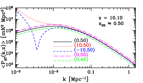
Figure 1: The spherically-averaged 21 cm power spectrum at $z=10.10$, using ESMR with the values of $(f_{NL},\zeta_{\rm ESMR})$ marked in the legend.

(i) ESMR: The basic postulate of ESMRFurlanetto04 is that the local ionized fraction within a spherical volume with radius $R$ is proportional to the local collapsed fraction of mass in luminous sources above some mass threshold $M_{\rm min}$, i.e. $x_{\rm HII}(M_{\rm min},R,z)=\zeta_{\rm ESMR}\,f_{\rm coll}(M_{\rm min},R,z)$, where $\zeta_{\rm ESMR}$ parametrizes the efficiency of this mass in releasing ionizing photons into the IGM. For simplicity, we assume atomic-cooling halos (ACHs), i.e.  halos with virial temperature $T_{\rm vir}\gtrsim 10^{4}\,{\rm K}$, are the only sources of ionizing radiation.

Our methodology for ESMR with PNG is as follows. The collapsed fraction of ACHs in Ref. D'Aloisio12 (see also Adshead12 ), calculated in the non-Markovian extension to the excursion set formalism Maggiore10a ; Maggiore10b ; Maggiore10c , for a given PNG parameter, is applied to the ESMR formalism to calculate the ionized density bias, for a given efficiency, analytically, as described in detail in Ref. D'Aloisio13 . Henceforth, since the functions $\bar{x}_{\rm HII}(z)$ and $b_{\rho_{\rm HII}}(k,z)$ are set by two parameters $(f_{NL},\,\zeta_{\rm ESMR})$, given a fiducial cosmology, so is the 21 cm power spectrum $P_{\Delta T}({\bf k},z)$ at any $z$. As Figure 1 illustrates, while $\zeta_{\rm ESMR}$ changes the amplitude of the 21 cm power spectrum, $f_{NL}$ changes the shape at small $k$ significantly. [Note that the reionization history is virtually independent of $f_{NL}$ for $\bar{x}_{\rm HII}>0.1$, e.g., for $\zeta_{\rm ESMR}=50$, $\bar{x}_{\rm HII}=0.50$ at $z=10.105\,(10.125)$ for $f_{NL}=0\,(10)$, respectively.] The (nonzero) minimum of the curve for $f_{NL}<0$ is at wavenumber $k_{\star}$, where $b_{\rho_{\rm HI}}(k_{\star},z)\approx-1/3$.

(ii) Phenomenological (“pheno”-) model: Just as PNG exhibits a scale-dependent effect on halo bias Dalal08 ; Matarrese08 ; Afshordi08 ; Desjacques11 ; Smith12 ; Adshead12 ; D'Aloisio12 ; Yokoyama12 , so we also find, in Ref. D'Aloisio13 , a scale-dependent non-Gaussian correction to the ionized density bias, $\Delta b^{(d)}_{\rho_{\rm HII}}(k,z)=b_{\rho_{\rm HII}}(k,z)-b^{\rm G}_{\rho_{\rm HII}}(z)$, where $b^{\rm G}_{\rho_{\rm HII}}$ is the Gaussian ionized density bias and scale-independent. [There is also a scale-independent non-Gaussian correction, $\Delta b^{(i)}_{\rho_{\rm HII}}(z)$. However, $\Delta b^{(i)}_{\rho_{\rm HII}}\ll b^{\rm G}_{\rho_{\rm HII}}$ for $f_{NL}<10$ (see D'Aloisio13 ), so we neglect it here, similar to the neglect of a scale-independent non-Gaussian correction to the halo bias when constraining PNG with galaxy surveys Giannantonio13 .]

For the local template, we derived from the ESMR a relation between $\Delta b^{(d)}_{\rho_{\rm HII}}$ and $b^{\rm G}_{\rho_{\rm HII}}$ in D'Aloisio13 . On large scales,

$$\Delta b^{(d)}_{\rho_{\rm HII}}(k,z)=3f_{NL}\left[b^{\rm G}_{\rho_{\rm HII}}(z)-1\right]\frac{\delta_{c}\Omega_{m}(H_{0}/c)^{2}}{g(0)D(z)k^{2}T(k)},$$ (3)

where $\delta_{c}\approx 1.686$ is the critical density in the spherical collapse model (in an Einstein-de Sitter universe); $D(z)$ is the linear growth factor normalized to unity at $z=0$; $g(0)=(1+z_{i})^{-1}D^{-1}(z_{i})\approx 0.76$ in our fiducial cosmology, where $z_{i}$ corresponds to the initial epoch, i.e. limit of large redshift; and $T(k)$ is the matter transfer function normalized to unity on large scales.

This relation was further tested and confirmed by numerical solution of the linear perturbation theory of reionization (LPTR) which includes radiative transfer Zhang07 . [For further details, see Ref. D'Aloisio13 .] Henceforth, Eq. (3) is assumed to be generic, regardless of reionization details. In what we call the “Pheno-model”, the 21 cm power spectrum is set by three parameters, $f_{NL}$, $\bar{x}_{\rm HI}$ and $b^{\rm G}_{\rho_{\rm HII}}$, at a given redshift. The latter two parameters embrace our ignorance of reionization.

Table 1: Specifications for 21 cm interferometers. We assume observation time $t_{0}=4000\,{\rm hours}$ for each redshift bin of bandwidth $B=6\,{\rm MHz}$.

Experiment	$N_{\rm in}$	$L_{\rm min}$ (m)	$\eta$	$A_{e}$($z=6/8/12$)[${\rm m}^{2}$]	$\Omega$[sr]
MWA	50	12.5	1	9/14/18	$\lambda^{2}/A_{e}$
LOFAR	32	100	0.8	397/656/1369	$2(\lambda^{2}/A_{e})$
SKA	1400	10	0.8	30/50/104	$\lambda^{2}/A_{e}$
Omniscope	$10^{6}$	1	1	1/1/1	$2\pi$

III Observability of 21 cm interferometric arrays using
Fisher matrix formalism

Radio interferometric arrays measure the 21 cm signal from coordinates ${\bf\Theta}\equiv\theta_{x}\hat{e}_{x}+\theta_{y}\hat{e}_{y}+\Delta\nu{\bf n}$, where $(\theta_{x},\theta_{y})$ mark the angular location on the sky, and $\Delta\nu$ is the frequency difference from the central redshift $z_{*}$ of a redshift bin. It is related to the 3D Cartesian coordinates ${\bf r}$ (with origin at the bin center) by ${\bf\Theta}_{\perp}={\bf r}_{\perp}/d_{A}(z_{*})$, and $\Delta\nu=r_{\parallel}/y(z_{*})$, where $d_{A}(z)$ is the comoving angular diameter distance, $y(z)\equiv\lambda_{21}(1+z)^{2}/H(z)$, $\lambda_{21}=\lambda(z)/(1+z)\approx 0.21\,{\rm m}$, and $H(z)$ is the Hubble parameter at $z$. The Fourier dual of ${\bf\Theta}$ is defined as ${\bf u}\equiv u_{x}\hat{e}_{x}+u_{y}\hat{e}_{y}+u_{\parallel}{\bf n}$ ($u_{\parallel}$ has units of time), which is related to ${\bf k}$ (Fourier dual to ${\bf r}$) by ${\bf u}_{\perp}=d_{A}{\bf k}_{\perp}$ and $u_{\parallel}=y\,k_{\parallel}$. The power spectrum in ${\bf u}$-space is related to that in the ${\bf k}$-space by $P_{\Delta T}({\bf u},z)=P_{\Delta T}({\bf k},z)/(d_{A}^{2}y)$.

For an interferometric array, a baseline ${\bf L}$ corresponds to ${\bf u}_{\perp}=2\pi{\bf L}/\lambda$. (Note: Our convention is different from the observer’s convention $u_{\perp}=L/\lambda$.) Let $\bar{n}({\bf L}_{\bf u_{\perp}})d^{2}{\bf L}$ denote the number of redundant baselines ${\bf L}_{\bf u_{\perp}}$ corresponding to ${\bf u_{\perp}}$, i.e. autocorrelation of array density. Then, the noise power spectrum in ${\bf u}$-space McQuinn06 ; Mao08 is $P^{N}({\bf u}_{\perp})=\left(\frac{\lambda T_{\rm sys}}{A_{e}}\right)^{2}/\left[t_{0}{\bar{n}}({\bf L}_{{\bf u}_{\perp}})\right]$, where $T_{\rm sys}\approx(280\,{\rm K})\left[(1+z)/7.4\right]^{2.3}$ is the system temperature Wyithe07 , $A_{e}\propto\lambda^{2}$ (for $\lambda$ less than antenna size) is effective collecting area, and $t_{0}$ is total observation time.

We adopt the following configuration of interferometric arrays. We assume antennas are concentrated within a nucleus of radius $R_{0}$ with area coverage fraction close to 100%, with coverage density dropping like $r^{-2}$ in a core extending from $R_{0}$ to $R_{\rm in}$. We neglect the dilute antenna distribution in the outskirts, $R>R_{\rm in}$. Given central array density $\rho_{0}$, the configuration can be specified by two convenient parameters: $N_{\rm in}$, the number of antennas within $R_{\rm in}$, and $\eta$, the fraction of these antennas that are in the nucleus . The relations are $R_{0}=\sqrt{\eta N_{\rm in}/\rho_{0}\pi}$, $R_{\rm in}=R_{0}\exp{[(1-\eta)/(2\eta)]}$ Mao08 .

Given a parameter space $\{p_{a}\}$, the Fisher matrix for 21 cm power spectrum measurements is ${\bf F}_{ab}=\sum_{\bf u}\left(\frac{\partial P_{\Delta T}({\bf u})}{\partial p_{a}}\right)\left(\frac{\partial P_{\Delta T}({\bf u})}{\partial p_{b}}\right)/\left[\delta P_{\Delta T}({\bf u})\right]^{2}$. The 1$\sigma$ forecast error of the parameter $p_{a}$ is given by $\Delta p_{a}=\sqrt{({\bf F^{-1}})_{aa}}$. The power spectrum measurement error in a pixel at ${\bf u}$ is $\delta P_{\Delta T}({\bf u})=\left[P_{\Delta T}({\bf u})+P_{N}(u_{\perp})\right]/\sqrt{N_{c}}$, where $N_{c}=u_{\perp}du_{\perp}du_{\parallel}\Omega B/(2\pi)^{2}$ is the number of independent modes in that pixel. We adopt logarithmic pixelization, $du_{\perp}/u_{\perp}=du_{\parallel}/u_{\parallel}=10\%$. Here, $\Omega$ is solid angle spanning the field of view, $B$ is bandwidth of the redshift bin.

We assume experimental specifications in Table 1, for MWAmwa , LOFARlofar , SKASKA , and OmniscopeFFTT , respectively. (We note that these interferometer array configurations were not designed to optimize the experiment proposed here, so improved constraints may be possible with other designs.) We assume residual foregrounds can be neglected for $k_{\parallel}\geq k_{\parallel,{\rm min}}=2\pi/(yB)$, e.g., $k_{\parallel,{\rm min}}=0.055\,{\rm Mpc}^{-1}$ at $z=10.1$. This foreground removal requirement is achievable, as demonstrated by, e.g.,McQuinn06 . (Ref. Lidz13 , submitted at about the same time as our paper, considers a somewhat more pessimistic foreground removal scenario in constraining PNG, complementary to our work.) The minimum $k_{\perp}$ is set by the minimum baseline, $k_{\perp,{\rm min}}=2\pi L_{\rm min}/(\lambda d_{A})$. We account for modes up to $k_{\rm max}=0.15\,{\rm Mpc}^{-1}$. Our fiducial cosmology is as follows: $\Omega_{\Lambda}=0.72$, $\Omega_{\rm M}=0.28$, $\Omega_{\rm b}=0.046$, $H_{0}=100h\,{\rm km}\,{\rm s}^{-1}\,{\rm Mpc}^{-1}$ ($h=0.7$), $\sigma_{8}=0.82$, $n_{\mathrm{s}}=0.96$, consistent with WMAP7 results Komatsu11 , with linear matter power spectrum of Ref. Eisenstein99 . ESMR fiducial values are $f_{NL}=0$, $\zeta_{\rm ESMR}=50.0$, corresponding to electron scattering optical depth $\tau_{\rm es}=0.08$. To facilitate direct comparison with ESMR, the fiducial model of 21 cm power spectrum for the Pheno-model will be the same as the ESMR fiducial model, which sets the fiducial values of $\bar{x}_{\rm HI}$ and $b^{\rm G}_{\rho_{\rm HII}}$ for a given redshift.

Table 2: Forecast 1$\sigma$ errors at $\bar{x}_{\rm HII}\approx 0.25$($z=11.24$) and $\bar{x}_{\rm HII}\approx 0.50$ ($z=10.10$), respectively. “F.V.” means fiducial values.

			ESMR		Pheno-model
$\bar{x}_{\rm HII}$			$f_{NL}$	$\zeta_{\rm ESMR}$	$f_{NL}$	$\bar{x}_{\rm HI}$	$b^{\rm G}_{\rho_{\rm HII}}$
		$\bigl{[}$F.V.	0	50.0	0	0.75	6.19 $\bigr{]}$
	MWA		13000	1500	14000	300	8800
$0.25$	LOFAR		1200	130	1200	1.1	29
	SKA		16	1.8	16	0.028	0.79
	Omniscope		0.38	0.040	0.38	0.00044	0.012
		$\bigl{[}$F.V.	0	50.0	0	0.50	5.43 $\bigr{]}$
	MWA		700	63	750	17	220
$0.50$	LOFAR		100	8.1	96	0.16	2.0
	SKA		19	1.5	18	0.030	0.37
	Omniscope		1.8	0.15	1.8	0.0023	0.027

IV Results

(i) Single epoch constraints: In Table 2, we list forecast errors, $\Delta f_{NL}$, marginalized over $\zeta_{\rm ESMR}$ in the ESMR, and over $\bar{x}_{\rm HI}$ and $b^{\rm G}_{\rho_{\rm HII}}$ in the Pheno-model. Top and bottom sets of forecasts use information from a single redshift bin centered at $z=11.24$ ($\bar{x}_{\rm HII}=0.25$) and $z=10.10$ ($\bar{x}_{\rm HII}=0.50$), respectively. For the same redshift and experiment, the values of $\Delta f_{NL}$ match very well between these two models. This demonstrates that the Pheno-model, which makes no assumptions about the connection between $\bar{x}_{\rm HI}$ and $b^{\rm G}_{\rho_{\rm HII}}$, can constrain $f_{NL}$ for a single epoch measurement as accurately as a reionization model which links the evolutions of $\bar{x}_{\rm HI}$ and $b^{\rm G}_{\rho_{\rm HII}}$.

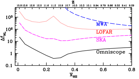
Figure 2: 1$\sigma$ error $\Delta f_{NL}$ from a series of single redshift bins, each with 6 MHz bandwidth.

For the same experiment, as Table 2 shows, values of $\Delta f_{NL}$ differ significantly between $\bar{x}_{\rm HII}=0.25$ and $0.50$, implying a strong dependence of $\Delta f_{NL}$ on $\bar{x}_{\rm HII}$. For Omniscope, in particular, $\Delta f_{NL}$ shrinks by a factor of $\sim 5$ from $\bar{x}_{\rm HII}=0.50$ to $0.25$. To investigate this in detail, we use the ESMR to plot $\Delta f_{NL}$ vs $\bar{x}_{\rm HII}$ in Figure 2. For MWA and LOFAR (both noise-dominated experiments), the constraint is tighter at higher $\bar{x}_{\rm HII}$ (i.e. lower redshift, where the noise is smaller). However, for SKA and Omniscope (cosmic-variance-dominated experiments), there appears to be a “sweet spot,” where $\Delta f_{NL}$ is minimized, at $\bar{x}_{\rm HII}\approx 0.25-0.30$. This sweet spot can be explained using the Pheno-model, as follows. The derivative $\left|dP_{\Delta T}/df_{NL}\right|\propto\left(\bar{x}_{\rm HII}/\bar{x}_{\rm HI}\right)\left[b^{\rm G}_{\rho_{\rm HII}}-1\right]\left|b^{\rm G}_{\rho_{\rm HI}}+\mu_{\bf k}^{2}\right|\propto\left|(1-b^{\rm G}_{\rho_{\rm HI}})(\frac{1}{3}+b^{\rm G}_{\rho_{\rm HI}})\right|$, using Eq. (2). In the ideal noise-free limit, the power spectrum error $\Delta P_{\Delta T}\propto P_{\Delta T}\propto\left[b^{\rm G}_{\rho_{\rm HI}}+\mu_{\bf k}^{2}\right]^{2}\approx{b^{\rm G}_{\rho_{\rm HI}}}^{2}+\frac{2}{3}\,b^{\rm G}_{\rho_{\rm HI}}+\frac{1}{5}$, when averaged over $\mu_{\bf k}$. Fixing $\bar{x}_{\rm HI}$ and $b^{\rm G}_{\rho_{\rm HII}}$, the Fisher matrix ${\bf F}=(\Delta f_{NL})^{-2}$ is peaked when $b^{\rm G}_{\rho_{\rm HI}}\approx-0.71$. Eq. (2) gives $\bar{x}_{\rm HII}=(1-b^{\rm G}_{\rho_{\rm HI}})/(b^{\rm G}_{\rho_{\rm HII}}-b^{\rm G}_{\rho_{\rm HI}})$. Since Gaussian bias $b^{\rm G}_{\rho_{\rm HII}}\approx 6$ (see Fig.5 of Ref.D'Aloisio13 ), the sweet spot is at $\bar{x}_{\rm HII}\approx 0.25$ in the ideal noise-free limit. In reality, finite noise is larger at higher redshifts, so the sweet spot will occur at slightly lower redshift.

Table 3: $\Delta f_{NL}$ from multiple redshift bins, marginalized over $\zeta_{\rm ESMR}$. “1-band,” “3-band,” “5-band,” “7-band” means the information of 1 bin (at $z=11.24$, $\bar{x}_{\rm HII}=0.25$), 3 bins ($\bar{x}_{\rm HII}\approx 0.17-0.37$), 5 bins ($\bar{x}_{\rm HII}\approx 0.11-0.52$), 7 bins ($\bar{x}_{\rm HII}\approx 0.06-0.70$), respectively.

Experiment	1-band	3-band	5-band	7-band
MWA	13000	1800	520	200
LOFAR	1215	91	39	26
SKA	16	5.0	3.5	2.8
Omniscope	0.38	0.23	0.18	0.16

(ii) Multi-epoch constraints: While a futuristic single epoch measurement can achieve a remarkable accuracy of $\Delta f_{NL}=0.38$ (16) for Omniscope (SKA), adding tomographic information can further improve the accuracy. The Pheno-model alone cannot be used to combine multi-frequency measurements because it does not specify the redshift evolutions of $\bar{x}_{\rm HI}$ and $b^{\rm G}_{\rho_{\rm HII}}$. On the other hand, a model such as the ESMR can be used to combine multi-frequency measurements because it fixes the reionization history (and therefore $P_{\Delta T}$) for a given ($f_{NL}$, $\zeta_{\rm ESMR}$). We show multi-epoch constraints from the ESMR in Table 3. Specifically, if information is combined from $\bar{x}_{\rm HII}\approx 0.06-0.70$ (7-band, total 42 MHz bandwidth, corresponding to $z\approx 9.5-13.4$ in the ESMR), the constraint can be significantly tightened, i.e. $\Delta f_{NL}=0.16$ for Omniscope (10 times smaller than an ideal CMB experiment), and $\Delta f_{NL}=2.8$ by SKA (two times smaller than Planck). A prior of $\Delta\tau_{\rm es}=0.014$ from Planck+WMAP CMB measurementsPlanck13cosmo corresponds to a prior of $\Delta\zeta_{\rm ESMR}\approx 39$, much larger than allowed by SKA and Omniscope alone, so adding this $\tau_{\rm es}$ prior cannot improve $\Delta f_{NL}$ from these experiments. If we take a more conservative upper limit, $k_{\rm max}=0.10\,{\rm Mpc}^{-1}$ (instead of $0.15\,{\rm Mpc}^{-1}$ as assumed above), then $\Delta f_{NL}$ for Omniscope is $\sim 2$ times larger. Since multi-epoch observations tighten $f_{NL}$ constraints by combining information from different frequency bands to increase the amount of data relative to a single band, our use of the simple ESMR model here, with constant efficiency parameter $\zeta_{\rm ESMR}$, for which reionization spans a relatively narrow range of redshift, may be a conservative one. If reionization is more extended, as in self-regulated reionization modelsIliev07 ; Iliev12 , for example, the resulting $f_{NL}$ constraints may be even tighter.

V Comparison with previous work

Previously, Ref. Joudaki11 reported forecasts of $\Delta f_{NL}=[100,700,50,4]$ for [MWA512, LOFAR, SKA, Omniscope] based on information from a single redshift bin at the 50%-ionized epoch. Their results can be compared to the bottom set in Table 2. Our results differ for a number of reasons: (1) Ref.Joudaki11 computed the scale-dependent signature of PNG in $P_{\Delta T}$ by fitting their approximate semi-numerical simulations of reionization. In Ref.D'Aloisio13 , we showed by our analytical derivation and numerical LPTR calculations that this fit underestimates the scale-dependent bias due to PNG significantly. These differences are reflected in the smaller $\Delta f_{NL}$ we obtain for LOFAR, SKA, and Omniscope. (2) The anticipated MWA512 configuration assumed by Ref. Joudaki11 was also overly optimistic, while we adopt the current MWA128 configuration mwa .

To model the effect of PNG on the 21 cm power spectrum, Ref. Chongchitnan13 assumed the simple functional dependence of ionized fraction on local overdensity, used for illustrative purposes by Ref. Alvarez06 for the Gaussian case, to derive an ionized fraction bias $b_{x}$ for PNG. Unfortunately, they incorrectly used $b_{x}$ to relate the 21 cm power spectrum to the matter power spectrum (see Ref. D'Aloisio13 ).

VI Conclusions

This paper suggests two approaches to constrain $f_{NL}$ with 21 cm power spectra from the EOR. If we take a conservative approach, i.e. assuming nothing about $\bar{x}_{\rm HI}(z)$ and $b_{\rho_{\rm HII}}^{G}(z)$, then the Pheno-model can be employed for a single redshift bin to provide $f_{NL}$ constraints with the same precision as a reionization model in which the reionization history is uniquely specified by a set of model parameters. However, using the ESMR, we demonstrate that a well-motivated reionization model can improve $\Delta f_{NL}$ in two ways: (1) a pathfinder measurement at a single redshift can best-fit the values of model parameters, which then can be used to estimate the desired redshift corresponding to $\bar{x}_{\rm HII}\approx 0.25-0.3$, i.e. the “sweet spot” for cosmic-variance-dominated experiments. This can help tune single-epoch observations for maximum precision. (2) Multi-epoch measurements can be combined to improve $\Delta f_{NL}$. We find that multi-frequency observation by SKA can achieve $\Delta f_{NL}\sim 3$, providing a new method to constrain PNG independent of CMB measurements, but with a precision comparable to Planck’s. A cosmic-variance-limited array of this size like Omniscope can achieve $\Delta f_{NL}\sim 0.2$, improving current constraints by an order of magnitude. These high precision observations may someday shed light on inflationary models.

- (1) A. H. Guth, Phys. Rev. D 23, 347 (1981)
- (2) A. D. Linde, Phys. Lett. B 108, 389 (1982)
- (3) A. D’Aloisio, J. Zhang, P. R. Shapiro, and Y. Mao, MNRAS, 433, 2900 (2013)
- (4) V. Acquaviva, N. Bartolo, S. Matarrese, A. Riotto Nuclear Physics B 667, 119 (2003)
- (5) J. Maldacena, Journal of High Energy Physics, 5, 13 (2003)
- (6) P. Creminelli, and M. Zaldarriaga, JCAP, 10, 6 (2004)
- (7) D. Seery, and J. E. Lidsey, JCAP, 6, 3 (2005)
- (8) X. Chen, M.-x. Huang, S. Kachru, G. Shiu, JCAP, 1, 2 (2007)
- (9) C. Cheung, A. L. Fitzpatrick, J. Kaplan, L. Senatore, JCAP, 2, 21 (2008)
- (10) P. A. R. Ade et al. [Planck Collaboration], ArXiv:1303.5076 (2013)
- (11) P. A. R. Ade et al. [Planck Collaboration], ArXiv:1303.5084 (2013)
- (12) E. Komatsu and D. N. Spergel, Phys. Rev. D 63, 063002 (2001)
- (13) D. Babich and M. Zaldarriaga, Phys. Rev. D 70, 083005 (2004)
- (14) S. Joudaki, O. Doré, L. Ferramacho, M. Kaplinghat, and M. G. Santos, Phys. Rev. Lett. 107, 131304 (2011)
- (15) S. Chongchitnan, JCAP, 03, 037 (2013)
- (16) R. Barkana and A. Loeb, ApJL, 624, L65 (2005)
- (17) Y. Mao, P. R. Shapiro, G. Mellema, I. T. Iliev, J. Koda, and K. Ahn, MNRAS, 422, 926 (2012)
- (18) P. R. Shapiro, Y. Mao, I. T. Iliev, G. Mellema, K. K. Datta, K. Ahn, and J. Koda, Phys. Rev. Lett. 110, 151301 (2013)
- (19) S. R. Furlanetto, M. Zaldarriaga, and L. Hernquist, Astrophys. J. , 613, 1 (2004)
- (20) A. D’Aloisio, J. Zhang, D. Jeong, P. R. Shapiro, MNRAS, 428, 2765 (2012)
- (21) P. Adshead, E. J. Baxter, S. Dodelson, and A. Lidz, Phys. Rev. D 86, 063526 (2012)
- (22) M. Maggiore and A. Riotto, ApJ, 711, 907 (2010)
- (23) M. Maggiore and A. Riotto, ApJ, 717, 515 (2010)
- (24) M. Maggiore and A. Riotto, ApJ, 717, 526 (2010)
- (25) N. Dalal, O. Doré, D. Huterer, and A. Shirokov, Phys. Rev. D 77, 123514 (2008)
- (26) S. Matarrese and L. Verde, ApJ, 677, L77 (2008)
- (27) N. Afshordi and A. J. Tolley, Phys. Rev. D 78, 123507 (2008)
- (28) V. Desjacques, D. Jeong, and F. Schmidt, Phys. Rev. D 84, 063512 (2011)
- (29) K. M. Smith, S. Ferraro, and M. LoVerde, JCAP, 3, 32 (2012)
- (30) S. Yokoyama and T. Matsubara, Phys. Rev. D 87, 023525 (2013)
- (31) T. Giannantonio, A. J. Ross, W. J. Percival, R. Crittenden, D. Bacher, M. Kilbinger, R. Nichol, and J. Weller, ArXiv:1303.1349 (2013)
- (32) J. Zhang, L. Hui, and Z. Haiman, MNRAS, 375, 324 (2007)
- (33) Y. Mao, M. Tegmark, M. McQuinn, M. Zaldarriaga, and O. Zahn, Phys. Rev. D 78, 023529 (2008)
- (34) M. McQuinn,O. Zahn, M. Zaldarriaga, L. Hernquist and S. R. Furlanetto, Astrophys. J. 653, 815 (2006)
- (35) S. Wyithe and M. F. Morales, ArXiv:astro-ph/0703070 (2007)
- (36) S. J. Tingay, et al. [MWA Collaboration], PASA, 30, 7 (2013); http://www.mwatelescope.org/.
- (37) M. P. van Haarlem et al. (in prep.), http://www.lofar.org
- (38) http://www.skatelescope.org/
- (39) M. Tegmark, and M. Zaldarriaga, Phys. Rev. D 79, 083530 (2009); M. Tegmark, and M. Zaldarriaga, Phys. Rev. D 82, 103501 (2010); S. Clesse, L. Lopez-Honorez, C. Ringeval, H. Tashiro, and M. H. G. Tytgat, Phys. Rev. D 86, 123506 (2012)
- (40) A. Lidz, E. J. Baxter, P. Adshead, and S. Dodelson, Phys. Rev. D 88, 023534 (2013).
- (41) E. Komatsu, et al. [WMAP Collaboration], ApJS, 192, 18 (2011)
- (42) D. J. Eisenstein and W. Hu, ApJ, 511, 5 (1999)
- (43) I. T. Iliev, G. Mellema, P. R. Shapiro, and U.-L. Pen, MNRAS, 376, 534 (2007)
- (44) I. T. Iliev, G. Mellema, P. R. Shapiro, and U.-L. Pen, Y. Mao, J. Koda, and K. Ahn, MNRAS, 423, 2222 (2012)
- (45) M. A. Alvarez, E. Komatsu, O. Doré, and P. R. Shapiro, ApJ, 647, 840 (2006)