Turbulence-Induced Relative Velocity of Dust Particles I: Identical Particles

Abstract

We study the relative velocity of inertial particles suspended in turbulent flows and discuss implications for dust particle collisions in protoplanetary disks. We simulate a weakly compressible turbulent flow, evolving 14 particle species with friction timescale, $\tau_{\rm p}$, covering the entire range of scales in the flow. The particle Stokes numbers, $St$, measuring the ratio of $\tau_{\rm p}$ to the Kolmogorov timescale, are in the range $0.1\;\hbox to0.0pt{\lower 2.5pt\hbox{$\sim$}\hss}\raise 1.5pt\hbox{$<$}\;St\;\hbox to0.0pt{\lower 2.5pt\hbox{$\sim$}\hss}\raise 1.5pt\hbox{$<$}\;800$. Using simulation results, we show that the model by Pan & Padoan (PP10) gives satisfactory predictions for the rms relative velocity between identical particles. The probability distribution function (PDF) of the relative velocity is found to be highly non-Gaussian. The PDF tails are well described by a 4/3 stretched exponential function for particles with $\tau_{\rm p}\simeq 1-2T_{\rm L}$, where $T_{\rm L}$ is the Lagrangian correlation timescale, consistent with a prediction based on PP10. The PDF approaches Gaussian only for very large particles with $\tau_{\rm p}\;\hbox to0.0pt{\lower 2.5pt\hbox{$\sim$}\hss}\raise 1.5pt\hbox{$>$}\;54T_{\rm L}$. We split particle pairs at given distances into two types with low and high relative speeds, referred to as continuous and caustic types, respectively, and compute their contributions to the collision kernel. Although amplified by the effect of clustering, the continuous contribution vanishes in the limit of infinitesimal particle distance, where the caustic contribution dominates. The caustic kernel per unit cross section rises rapidly as $St$ increases toward $\simeq 1$, reaches a maximum at $\tau_{\rm p}\simeq 2T_{\rm L}$, and decreases as $\tau_{\rm p}^{-1/2}$ for $\tau_{\rm p}\gg T_{\rm L}$.

1. Introduction

The dynamics of particles of finite inertia suspended in turbulent flows is a fundamental problem with applications ranging from industrial processes (e.g. spray combustion engines) to geophysical flows (e.g., atmospheric clouds). The interaction between turbulence and particles has been studied to understand rain initiation in warm terrestrial clouds (e.g., Pinsky & Khain 1997; Falkovich, Fouxon,& Stepanov 2002; Shaw 2003), cloud evolution in the atmospheres of planets, cool stars and brown dwarfs (e.g., Rossow 1978; Pruppacher & Klett 1997; Freytag et al. 2010; Helling et al. 2011), collisions and growth of dust particles in protoplanetory disks (e.g., Dullemond & Dominik 2005; Zsom et al. 2010, 2011; Birnstiel et al. 2011) and in the interstellar medium (e.g., Ormel et al. 2009).

The evolution of the particle size depends on the particle collision rate which may be significantly enhanced by turbulent motions in the carrier flow, as illustrated by recent numerical and theoretical advances in this field (e.g., Wang et al. 2000; Zhou et al. 2001; Falkovich et al. 2002; Zaichik & Alipchenkov 2003, 2009; Zaichik et al.  2003, 2006; Wilkinson et al. 2005, 2006; Falkovich & Pumir 2007; Gustavsson & Mehlig 2011; Gustavsson et al. 2012). An accurate evaluation of the collision rates requires understanding the effects of two interesting phenomena: the preferential concentration or clustering of inertial particles (e.g., Maxey 1987 and Squires & Eaton 1991) and the turbulence-induced collision velocity. In this work, we will focus on the statistics of turbulence-induced relative velocities, and briefly discuss the role of turbulent clustering on the collision rate (see Pan et al. 2011 for a detailed discussion of turbulent clustering in the context of planetesimal formation). We restrict our discussion to the relative velocity between same-size particles, usually referred to as the monodisperse case, and will address the general bidisperse case (collisions between particles of different sizes) in a follow-up paper.

The main motivation of our study is to improve the modeling of the evolution of dust particles in protoplanetary disks, which sets the stage for the formation of planetesimals, the likely precursors to fully-fledged planets. For example, the planetesimal formation model by Johansen et al. (2007, 2009, 2011) requires particle growth up to decimeter to meter size, in order to achieve good frictional coupling to the disk rotation and hence the maximum clustering effect by the streaming instability. Cuzzi et al. (2008, 2010) and Chambers (2010) proposed an alternative model of planetesimal formation based on the strong turbulent clustering of chondrule-size particles. Other studies (e.g. Lee et al. 2010) focus on the possibility that small particles settle to the disk midplane, where gravitational instability can result in planetesimal formation (e.g. Goldreich & Ward 1973; Youdin 2011), despite the turbulence stirring caused by the Kelvin-Helmholtz instability induced by the vertical settling of the particles (e.g. Weidenschilling 1980; Chiang 2008).

The evolution of the size distribution of dust particles is controlled by collisions. Small particles tend to stick together when colliding, and thus their size grows by coagulation. As the size increases, the particles become less sticky (Blum & Wurm 2010), and, depending on the collision velocity, the collisions may result in bouncing or fragmentation. A detailed summary of experimental results for the dependence of the collision outcome on the particle properties (such as the particle size and porosity) and on the collision velocity can be found in Guttler et al. (2010). The coagulation, bouncing and fragmentation processes may lead to a quasi-equilibrium distribution of particle sizes (e.g., Birnstiel et al. 2011; Zsom et al. 2010, 2011). Due to the dependence of the collision outcome on the collision velocity, an accurate evaluation of the turbulence-induced relative velocity is important for modeling the size distribution of dust particles.

Saffman and Turner (1956) studied the relative velocity in the limit of small particles with the particle friction or stopping time, $\tau_{\rm p}$, much smaller than the Kolmogorov timescale, $\tau_{\eta}$, of the turbulent flow. This limit, known as the Saffman-Turner limit, is usually expressed as $St\ll 1$, where the Stokes number is defined as $St\equiv\tau_{\rm p}/\tau_{\eta}$. Saffman and Turner (1956) predicted that, at a given distance, $r$, the relative velocity of identical particles is independent of $St$, and, at a given $St$, it scales linearly with $r$ for small $r$. In the opposite limit of large particles with $\tau_{\rm p}$ larger than the largest timescale of the turbulent flow, Abrahamson (1975) showed that the relative velocity scales with the friction time as $\tau_{\rm p}^{-1/2}$. A variety of models have been developed to bridge the two limits and to predict the relative velocity for particles of any size, i.e., with $\tau_{\rm p}$ covering the entire scale range of the carrier flow (Williams & Crane 1983, Yuu 1984, Kruis & Kusters 1997, & Alipchenkov 2003, Zaichik et al. 2006, Ayala et al. 2008). Among these models, the formulation of Zaichik and collaborators is particularly impressive, as it examines turbulent clustering and turbulence-induced relative velocity simultaneously. The model prediction for the relative velocity agrees well with simulation results at low resolutions. However, the model lacks a transparent physical picture.

Pan & Padoan (2010) developed a new model for the relative velocity of inertial particles of any size that provides an insightful physical picture of the problem. Their formulation illustrates that the relative velocity of identical particles is determined by the memory of the flow velocity difference along their trajectories in the past. The model also shows that the separation of inertial particle pairs backward in time plays an important role in their relative velocity. The model prediction can correctly reproduce the scaling behaviors of the relative speed in the extreme limits of small and large particles, and was found to successfully match the simulation data of Wang et al. (2000).

Falkovich et al. (2002) discovered an interesting effect, named the sling effect, which provides an important contribution to the collision rate. The basic physical picture of this effect is that inertial particles may be shot out of fluid streamlines with high curvature, causing their trajectories to cross with those of other particles (see Fig. 1 of Falkovich & Pumir 2007). In particular, in flow regions with large negative velocity gradients, fast particles can catch up with the slower ones from behind. The trajectory crossing causes the particle velocity to be multi-valued at a given point. This gives rise to folds, usually referred to as caustics, in the momentum-position phase space of the particles (Wilkinson et al. 2006; see Fig. 1 of Gustavsson & Mehlig 2011 for a clear illustration). For small particles with $St\ll 1$, the sling events correspond to high-order statistics of the flow velocity gradient, and the effect is not reflected in the prediction of Saffman and Turner (1956). The formulations of Falkovich et al. (2002) and Gustavsson & Mehlig (2011) for the collision kernel of $St\;\hbox to0.0pt{\lower 2.5pt\hbox{$\sim$}\hss}\raise 1.5pt\hbox{$<$}\;1$ particles consist of two contributions. Following Wilkinson et al. (2006), we name them as continuous and caustic contributions, corresponding to two types of particle pairs with low and high relative velocities, respectively. In the continuous contribution, the relative speed follows the Saffman-Turner prediction and decreases linearly with the particle distance, $r$. The contribution is amplified by turbulent clustering. However, the scaling exponents of the relative speed and the degree of clustering suggest that the continuous contribution approaches zero in the limit $r\to 0$, as pointed out by Hubbard (2012). The caustic contribution to the collision kernel per unit cross section was predicted to be independent of the particle size or distance, $r$, and is thus expected to dominate at sufficiently small $r$. The effect of slings or caustics causes a rapid rise in the collision rate as $St$ approaches 1, which has been proposed to be responsible for the initiation of rain shower in terrestrial clouds (Wilkinson et al. 2006). Applying this effect to dust particle collisions in protoplanetary disks, one may expect that the collision rate greatly accelerates as the particle grows past sub-mm to mm size, corresponding to $St\simeq 1$ for typical protoplanetary turbulence conditions.

The recent developments mentioned above have not been considered in coagulation models for dust particles in circumstellar disks. We will show that the general formulation of the collision kernel commonly used in the astrophysical literature for dust coagulation is inaccurate. In particular, the dust coagulation models usually adopt collision velocities from the work of Volk et al. (1980) and its later extensions (e.g., Markiewicz, Mizuno & Volk 1991, Cuzzi and Hogan 2003, and Ormel & Cuzzi 2007), which have a number of limitations. Pan & Padoan (2010) pointed out a weakness in the physical picture of these models. Roughly speaking, these models assume that the velocities of two particles induced by turbulent eddies with turnover time significantly smaller (larger) than $\tau_{\rm p}$ are independent (correlated). As shown by Pan & Padoan (2010), whether the particle velocities contributed by turbulent eddies of a given size are correlated or not also depends on how the eddy size compares to the separation of the particles at the time the eddies were encountered. Therefore, the eddy turnover time is not the only factor that determines the degree of correlation. The role of the particle separation relative to the eddy size is not captured by the approach of Volk et al. We also find that the model of Volk et al. overestimates the relative velocity by a factor of 2 for particles with $\tau_{\rm p}$ on the order of the large eddy turnover time of the turbulent flow.

In this paper, we conduct a $512^{3}$ numerical simulation to study inertial particle dynamics in a hydrodynamic turbulent flow. In the simulated flow, we evolve inertial particles in an extended size range, with $\tau_{\rm p}$ covering the entire scale range of the turbulent flow. To our knowledge, such a systematic simulation of a significant resolution has not been previously conducted in the astrophysical literature. Using the simulation data, we first test the model prediction of Pan & Padoan (2010) for the rms relative velocity of inertial particles as a function of $St$, and validate the physical picture revealed by the model. We then apply the Pan & Padoan (2010) model to interpret the probability distribution function (PDF) of the relative velocity. The PDF study is motivated by the importance of the PDF of the collision speed in modeling dust particle collisions (Windmark et al. 2012, Garaud et al. 2013), which determines the fractions of collisions leading to sticking, bouncing or fragmentation. The relative velocity PDF of inertial particles has been shown to be highly non-Gaussian by numerical, experimental and theoretical studies (e.g., Sundaram and Collins 1997, Wang et al. 2000, Gustavsson et al. 2008, Bec et al. 2009, de Jong et al. 2010, Gustavsson & Mehlig 2011, Hubbard 2012). Our simulation further confirms high non-Gaussianity, which should be incorporated into coagulation models for dust particles in protoplanetary disks. We will also investigate the particle collision kernel as a function of $St$.

Due to the computational cost, the number of particles included in our simulation is limited and only allows to accurately measure the relative velocity statistics at significant particle distances. The distance range explored is $\eta/4\leq r\leq\eta$ where $\eta$ is the Kolmogorov scale of the simulated flow. This raises the question concerning the direct applicability of our measured statistics to dust particle collisions. The size of dust particles is many orders of magnitudes smaller than the Kolmogorov scale ($\eta\sim 1$ km) in protoplanetary turbulence. Therefore, dust particles should be viewed as nearly point particles, and one is required to examine the $r\to 0$ limit in order to model their collisions (Hubbard 2012, 2013). This suggests that the relative velocity measured in our simulation at $r\simeq\eta$ would be distinct from the collision speed of dust particles, unless the statistics have already converged at $\simeq\eta$. We find that the measured relative velocity statistics for particles with $St\;\hbox to0.0pt{\lower 2.5pt\hbox{$\sim$}\hss}\raise 1.5pt\hbox{$>$}\;10$ actually converge at $r\simeq\eta$, and are thus directly applicable for the collision velocity of dust particles. On the other hand, for small to intermediate particles with $St\;\hbox to0.0pt{\lower 2.5pt\hbox{$\sim$}\hss}\raise 1.5pt\hbox{$<$}\;10$, the measured statistics show an $r$-dependence in the $r$ range explored in this study. For these particles, an appropriate extrapolation to the $r\to 0$ limit is needed for applications to dust particle collisions.

In the current paper, we focus on understanding the fundamental physics of turbulence-induced relative velocity at finite distances ($\;\hbox to0.0pt{\lower 2.5pt\hbox{$\sim$}\hss}\raise 1.5pt\hbox{$<$}\;1\eta$). Our theoretical and numerical results provide an important step toward the final goal of estimating the dust particle collision velocity at $r\to 0$. To underhand the $r\to 0$ limit, we make an initial and preliminary attempt to separate particle pairs into two types, i.e., continuous and caustic types, which show different scalings with $r$. In particular, we evaluate the contributions of two types of pairs to the collision kernel and examine their behaviors as $r\to 0$. A systematical study for the $r\to 0$ limit is deferred to a future work.

In this work, we will consider the particle dynamics only in statistically homogeneous and isotropic turbulence. This is clearly an idealized situation, considering various complexities in protoplanetary disks. For example, the disk rotation induces large-scale anisotropy, which may have significant effects on the prediction for particles with friction time close to the rotation period. Nevertheless, the idealized problem is a very useful tool to understand the fundamental physics. We also neglect the vertical settling and radial drift. These processes do not directly affect the relative velocity between identical particles, although they may provide important contributions for particles of different sizes that we address in a follow-up work.

The paper is organized as follows. In §2, we present a simple model for the rms velocity of a single particle, which provides an illustration for our formulation of the particle relative velocity. In §3, we introduce the model of Pan & Padoan (2010) for the relative velocity of nearby particles. Our simulation setup and the statistical properties of the simulated turbulent flow are described in §4. §5 presents simulation results for the one-particle rms velocity. In §6, we test the model prediction of Pan & Padoan (2010) for the rms relative velocity, and discuss in details the probability distribution of the relative velocity as a function of the particle inertia. In §7, we evaluate the collision kernel. The conclusions of our study are summarized in §8.

2. The Velocity of Inertial Particles

The dynamics of inertial particles depends crucially on its friction or stopping timescale, $\tau_{\rm p}$. To evaluate of the friction timescale, we first need to compare the particle size, $a_{\rm p}$, with the mean free path of the gas particles in the carrier flow. If the particle size is larger than the mean free path, the friction timescale is given by the Stokes law $\tau_{\rm p}=\frac{2}{9}\left(\frac{\rho_{\rm d}}{\rho}\right)\left(\frac{a_{\rm p}^{2}}{\nu}\right)$, where $\rho_{\rm d}$ ($\simeq 1$ g cm^-3) is the density of the dust material, $\rho$ is the gas density, and $\nu$ is the kinematic viscosity of the flow. On the other hand, if $a_{\rm p}$ is smaller than the gas mean free path, the particle is in the Epstein regime and $\tau_{\rm p}=\left(\frac{\rho_{\rm d}}{\rho}\right)\left(\frac{a_{\rm p}}{C_{\rm s}}\right)$, where $C_{\rm s}$ is the sound speed in the flow. For example, for a typical gas density in protoplanetary discs, $\rho\simeq 10^{-9}$ g cm^-3, at 1 AU, the mean free path of the gas particles is $\sim 1$ cm, and thus particles with $a_{\rm p}$ larger (smaller) than 1 cm are in the Stokes (Epstein) regime.

The velocity, ${\boldsymbol{v}}(t)$, of an inertial particle suspended in a turbulent velocity field, $\boldsymbol{u}({\boldsymbol{x}},t)$, obeys the equation,

$$\frac{d{\boldsymbol{v}}}{dt}=\frac{{\boldsymbol{u}}\left({\boldsymbol{X}}(t),t\right)-{\boldsymbol{v}}}{\tau_{\rm p}},$$ (1)

where ${\boldsymbol{X}}(t)$ is the position of the particle at time $t$, and ${\boldsymbol{u}}\left({\boldsymbol{X}}(t),t\right)$ corresponds to the flow velocity “seen” by the particle. Eq. (1) has a formal solution,

$${\boldsymbol{v}}(t)=\frac{1}{\tau_{\rm p}}\int_{t_{0}}^{t}{\boldsymbol{u}}\left({\boldsymbol{X}}(\tau),\tau\right)\exp\left(-\frac{t-\tau}{\tau_{\rm p}}\right)d\tau,$$ (2)

where it is assumed that $t-t_{0}\gg\tau_{\rm p}$ and the particle has already lost the memory of its initial velocity at $t_{0}$. The formal solution indicates that the velocity of an inertial particle is determined by the memory of the flow velocity along its trajectory within a timescale of $\simeq\tau_{\rm p}$ in the past.

Although the aim of the present work is the relative velocity of inertial particle pairs, we start with a discussion of the single-particle (or “1-particle”) velocity induced by turbulent motions. We provide a simple model for the 1-particle rms velocity as a function of $\tau_{\rm p}$. The derivation of this model helps to illustrate our formulation for the relative velocity between two nearby particles.

The 1-particle rms velocity can be calculated using the formal solution of eq. (2). We assume the turbulent flow is statistically stationary, and the particle statistics eventually relax to a steady state. We consider a time when the steady state is already reached and denote this time as time 0. Using eq. (2) at $t=0$, we have,

$$\langle v_{i}v_{j}\rangle=\int_{-\infty}^{0}\frac{d\tau}{\tau_{\rm p}}\int_{-\infty}^{0}\frac{d\tau^{\prime}}{\tau_{\rm p}}B_{{\rm T}ij}(\tau,\tau^{\prime})\exp\left(\frac{\tau}{\tau_{\rm p}}\right)\exp\left(\frac{\tau^{\prime}}{\tau_{\rm p}}\right),$$ (3)

where $\langle\cdot\cdot\cdot\rangle$ denotes the ensemble average and $B_{{\rm T}ij}(\tau,\tau^{\prime})\equiv\left\langle u_{i}({\boldsymbol{X}}(\tau),\tau)u_{j}({\boldsymbol{X}}(\tau^{\prime}),\tau^{\prime})\right\rangle$ is the temporal correlation tensor of the flow velocity along the trajectory, ${\boldsymbol{X}}(\tau)$, of the inertial particle. The subscript “T” stands for “trajectory”. We changed the lower integration limit ($t_{0}$) in eq. (2) to $-\infty$, based on the assumption that the particle dynamics is fully relaxed at time 0 (i.e., $t_{0}\ll-\tau_{\rm p}$).

With statistical stationarity and isotropy, the trajectory correlation tensor can be written as $B_{{\rm T}ij}(\tau,\tau^{\prime})=u^{\prime 2}\Phi_{\rm 1}(\tau^{\prime}-\tau)\delta_{ij}$, where $u^{\prime}$ is the 1D rms velocity of the turbulent flow and the correlation coefficient $\Phi_{\rm 1}$ is a function of the time lag only. The subscript “1” is used to indicate that the correlation is along the trajectory of one particle. The correlation coefficient, $\Phi_{\rm 1}$, is unknown, and a common assumption is to approximate it with the Lagrangian correlation function, $\Phi_{\rm L}$, of tracer particles (or fluid elements), which has been extensively studied. The assumption is likely valid for small particles, but cannot be justified for large particles on a theoretical basis. We will validate the assumption a posteriori using simulation results.

The simplest choice for $\Phi_{\rm L}$ is an exponential function, $\Phi_{\rm L}(\Delta\tau)=\exp(-|\Delta\tau|/T_{\rm L})$, where $\Delta\tau=\tau^{\prime}-\tau$ is the time lag and $T_{\rm L}$ the Lagrangian correlation timescale. Setting $B_{{\rm T}ij}=u^{\prime 2}\exp(-|\tau^{\prime}-\tau|/T_{\rm L})\delta_{ij}$ in eq. (3), we have $\langle v_{i}v_{j}\rangle=v^{\prime 2}\delta_{ij}$, where the 1D rms particle velocity, $v^{\prime}$, is given by,

$$v^{\prime}=u^{\prime}\left(\frac{T_{\rm L}}{T_{\rm L}+\tau_{\rm p}}\right)^{1/2}.$$ (4)

This result shows that the particle rms velocity approaches the flow velocity for $\tau_{\rm p}\ll T_{\rm L}$ and decreases as $(T_{\rm L}/\tau_{\rm p})^{1/2}$ for $\tau_{\rm p}\gg T_{\rm L}$ (e.g., Abrahamson 1975). In the large particle limit, $\tau_{\rm p}\gg T_{\rm L}$, the action of even the largest turbulent eddies on the particle would appear to be random kicks when viewed on a timescale of $\tau_{\rm p}$. In that case, eq. (1) is essentially a Langevin equation, and the particle motions are similar to Brownian motions. The $\tau_{\rm p}^{-1/2}$ scaling corresponds to an “equilibrium” between the velocity of these particles and the turbulent motions of the flow.

Numerical simulations have shown that the Lagrangian correlation function, $\Phi_{\rm L}(\Delta\tau)$, is better fit by a bi-exponential form (e.g., Sawford 1991). A single-exponential form does not reflect the smooth part of the correlation function for $\Delta\tau$ smaller than the Taylor micro timescale, $\tau_{\rm T}$. The Taylor timescale is defined as $\left(2u^{\prime 2}/a^{2}\right)^{1/2}$, where $a$ is the rms acceleration of the turbulent velocity field. The bi-exponential form for $\Phi_{\rm L}(\Delta\tau)$ is,

$$\hskip 28.45274pt\exp\Bigg{[}-\frac{2|\Delta\tau|}{\big{(}1+\sqrt{1-2z^{2}}\big{)}T_{\rm L}}\Bigg{]}-\big{(}1-\sqrt{1-2z^{2}}\big{)}\times$$

$$\exp\left[{-\frac{2|\Delta\tau|}{\big{(}1-\sqrt{1-2z^{2}}\big{)}T_{\rm L}}}\right]\bBigg@{3}\},\hskip 51.21504pt$$ (5)

where the parameter $z$ is defined as $z=\tau_{\rm T}/T_{\rm L}$. From the above equation, it is easy to show that $T_{\rm L}=\int\Phi_{\rm L}(\Delta\tau)d\Delta\tau$, and the bi-exponential function is smooth, $\simeq 1-(\Delta\tau/\tau_{\rm T})^{2}$, at $\Delta\tau\ll\tau_{\rm T}$. In the limit $z\to 0$, eq. (5) reduces to the single exponential with a timescale of $T_{\rm L}$.

Adopting the bi-exponential form, eq. (5), for the trajectory correlation coefficient, $\Phi_{1}$, we find that the 1-particle rms velocity is given by,

$$v^{\prime}=u^{\prime}\left(\frac{\Omega+z^{2}/2}{\Omega+\Omega^{2}+z^{2}/2}\right)^{1/2},$$ (6)

where $\Omega$ is defined as $\Omega\equiv\tau_{\rm p}/T_{\rm L}$. In the limits $\Omega\ll 1$ and $\Omega\gg 1$, eq. (6) has the same behavior as eq. (4) from the single exponential correlation. In fact, the two predictions, eqs. (4) and (6), are close to each other at all values of $\Omega$, differing only by a few percent at $\Omega\simeq 1$. This suggests that, for a given correlation timescale, $T_{\rm L}$$(\equiv\int\Phi_{\rm L}(\Delta\tau)d\Delta\tau$), the integral in eq. (3) is insensitive to the exact function form of $\Phi_{1}(\Delta\tau)$. We will measure $z$ and $T_{\rm L}$ using Lagrangian tracer particles in our simulated turbulent flow, and test the predictions, eqs. (4) and (6), against the simulation data.

3. Turbulence-induced Relative Velocity of Inertial Particles

We briefly review the 2-point Eulerian statistics of the velocity field in fully-developed turbulence, which is crucial to understand the relative velocity of two inertial particles. We consider the structure tensor of a turbulent flow, defined as $S_{ij}(\boldsymbol{\ell})=\left\langle\Delta u_{i}\Delta u_{j}\right\rangle$ where $\Delta u_{i}=u_{i}({\boldsymbol{x}}+{\boldsymbol{\ell}},t)-u_{i}({\boldsymbol{x}},t)$ is the velocity increment across a separation ${\boldsymbol{\ell}}$. The statistics of $\Delta u_{i}$ is independent of ${\boldsymbol{x}}$ and $t$ from the assumption of homogeneity and stationarity. With statistical isotropy, the velocity structure tensor takes the form (e.g., Monin and Yaglom 1975),

$$S_{ij}(\boldsymbol{\ell})=S_{\rm nn}(\ell)\delta_{ij}+\left[S_{\rm ll}(\ell)-S_{\rm nn}(\ell)\right]\frac{\ell_{i}\ell_{j}}{\ell^{2}}$$ (7)

where the longitudinal and transverse structure functions, $S_{\rm ll}$ and $S_{\rm nn}$, are functions of the amplitude, $\ell$, but not the direction (${\boldsymbol{\ell}}/\ell$) of ${\boldsymbol{\ell}}$. From eq. (7), we see $S_{\rm ll}=S_{ij}(\boldsymbol{\ell})\ell_{i}\ell_{j}/\ell^{2}=\left\langle\Delta u_{\rm r}^{2}\right\rangle$, where $\Delta u_{\rm r}=\Delta u_{i}\ell_{i}/\ell$ is the radial component of ${\boldsymbol{\Delta}u}$. Similarly, $S_{\rm nn}$ can be written as $S_{\rm nn}=\langle(\Delta u_{\rm t})^{2}\rangle$ with $\Delta u_{\rm t}$ being one of the two components of ${\boldsymbol{\Delta}u}$ on the tangential/transverse plane perpendicular to ${\boldsymbol{\ell}}$. The statistical isotropy indicates that the probability distribution of $\Delta u_{\rm t}$ is invariant under any rotation about the direction ${\boldsymbol{\ell}}/\ell$. In incompressible turbulence, which is approximately the case for gas flows in protoplanetary disks, we have the relation $S_{\rm nn}=S_{\rm ll}+\frac{1}{2}{\ell}dS_{\rm ll}/d\ell$, which can be derived from the incompressibility condition: $\partial_{j}S_{ij}({\boldsymbol{\ell}})=0$ (Monin and Yaglom 1975).

The structure functions exhibit different scaling behaviors in different scale ranges. There are three subranges divided by two length scales, the Kolmogorov length scale, $\eta$, and the integral length scale $L$. The Kolmogorov scale, $\eta$, is defined as $\eta=(\nu^{3}/\bar{\epsilon})^{1/4}$, where $\nu$ and $\bar{\epsilon}$ are, respectively, the kinematic viscosity and the average energy dissipation rate in the turbulent flow. It essentially corresponds to the size of the smallest eddies. Scales below $\eta$ are called the viscous or dissipation range, where the velocity field is laminar and differentiable due to the smoothing effect of the viscosity. In the dissipation range, the velocity difference scales linearly with $\ell$, and the longitudinal structure function is $S_{\rm ll}=\frac{\bar{\epsilon}}{15\nu}\ell^{2}$. $S_{\rm nn}$ is twice larger, i.e., $S_{\rm nn}=\frac{2\bar{\epsilon}}{15\nu}\ell^{2}$, as required by the incompressibility constraint. In the inertial range, $\eta\;\hbox to0.0pt{\lower 2.5pt\hbox{$\sim$}\hss}\raise 1.5pt\hbox{$<$}\;\ell\;\hbox to0.0pt{\lower 2.5pt\hbox{$\sim$}\hss}\raise 1.5pt\hbox{$<$}\;L$, $S_{\rm ll}$ follows the Kolmogorov scaling, $S_{\rm ll}=C_{\rm K}(\bar{\epsilon}\ell)^{2/3}$, where $C_{\rm K}$ is the Kolmogorov constant. The typical value of $C_{\rm K}$ is $\simeq 2$. The incompressibility condition gives $S_{\rm nn}=4S_{\rm ll}/3$ in the inertial range. The integral scale, $L$, is essentially the correlation length of the velocity field. At $\ell\gg L$, the velocity field is uncorrelated, and both $S_{\rm ll}(\ell)$ and $S_{\rm nn}(\ell)$ are constant and equal to $2u^{\prime 2}$ with $u^{\prime}$ the 1D rms velocity of the flow.

To bridge the scalings of $S_{\rm ll}$ in the three scale ranges, we adopt a connecting formula (Zaichik et al.  2006),

$${\displaystyle S_{\rm ll}=2u^{\prime 2}\left[1-\exp\left(-\frac{(\ell/\eta)}{(15C_{\rm K})^{3/4}}\right)\right]^{4/3}\times}\hskip 56.9055pt$$

$$\hskip 85.35826pt{\displaystyle\left[\frac{(\ell/\eta)^{4}}{(\ell/\eta)^{4}+(2u^{\prime 2}/C_{\rm K}u_{\eta}^{2})^{6}}\right]^{1/6}},$$ (8)

where $u_{\eta}$ is the Kolmogorov velocity scale defined as $(\nu\bar{\epsilon})^{1/4}$. With eq. (8) for $S_{\rm ll}$, we can obtain $S_{\rm nn}$ using the incompressibility condition (see above). Alternatively, one may adopt a separate connecting formula for $S_{\rm nn}$ (see §4.3).

The goal of this work is to understand the relative velocity of two nearby inertial particles. The relative velocity across a distance, $r$, equal to the sum of the particle radii corresponds to the speed at which the two particles collide (Saffman and Turner 1956). As mentioned earlier, dust particles in protoplanetary disks are nearly point-like, as their size is much smaller than the Kolmogorov length scale, $\eta$. The collision speed of dust particles is therefore the relative velocity at $r\to 0$. In this paper, we focus on the relative speed at finite distances, $r\;\hbox to0.0pt{\lower 2.5pt\hbox{$\sim$}\hss}\raise 1.5pt\hbox{$<$}\;\eta$, and the $r\to 0$ limit will be examined systematically in a future work.

We label two particles coming together with superscripts $(1)$ and $(2)$. For example, we denote their positions as ${\boldsymbol{X}}^{(1)}(t)$ and ${\boldsymbol{X}}^{(2)}(t)$, and their velocities as ${\boldsymbol{v}}^{(1)}(t)$ and $\boldsymbol{v}^{(2)}(t)$ (see Fig. 1 for illustration). When the superscripts $(1)$ and $(2)$ are not used, the discussion is general and not referring to a specific particle. At a given time $t$, we consider the relative velocity ${\boldsymbol{w}}\equiv{\boldsymbol{v}}^{(2)}(t)-{\boldsymbol{v}}^{(1)}(t)$, of particle pairs at a given separation, ${\boldsymbol{r}}$, which corresponds to a constraint ${\boldsymbol{X}}^{(2)}(t)-{\boldsymbol{X}}^{(1)}(t)={\boldsymbol{r}}$ for the particle positions. We first present a theoretical model for the second-order moment of ${\boldsymbol{w}}$, and then use simulations to explore its full statistics including the probability distribution function (PDF).

Similar to the structure tensor of the flow velocity, we characterize the second-order statistics of the particle relative velocity ${\boldsymbol{w}}$ by a structure tensor,

$$S_{{\rm p}ij}\equiv\left\langle w_{i}w_{j}\right\rangle=\left\langle\left(v^{(2)}_{i}-v^{(1)}_{i}\right)\left(v^{(2)}_{j}-v^{(1)}_{j}\right)\right\rangle,$$ (9)

which was referred to as the particle velocity structure tensor by Pan and Padoan (2010). Here $\langle\cdot\cdot\cdot\rangle$ denotes the average over all particle pairs at a separation of ${\boldsymbol{r}}$.

Once the particle dynamics is fully relaxed, the particle velocity is expected to possess the same statistical symmetries as the flow, including stationarity, homogeneity and isotropy. With these symmetries, $S_{{\rm p}ij}$ can be written in a similar form as the structure tensor of the flow (eq. 7),

$$S_{{\rm p}ij}({\boldsymbol{r}})=\langle w_{\rm t}^{2}\rangle\delta_{ij}+\left(\langle w_{\rm r}^{2}\rangle-\langle w_{\rm t}^{2}\rangle\right)\frac{r_{i}r_{j}}{r^{2}},$$ (10)

where $\langle w_{\rm r}^{2}\rangle$ and $\langle w_{\rm t}^{2}\rangle$ are the variances of the radial/longitudinal component, $w_{\rm r}$ ($\equiv w_{i}r_{i}/r$), and a tangential/transverse component, $w_{\rm t}$, of the relative velocity, respectively. For particle collisions, we are interested in $S_{{\rm p}ij}$ at small distances only, with $r$ in the dissipation range of the flow. Under the assumption of isotropy, the tangential component, $w_{\rm t}$, is expected to be statistically invariant for any rotations about the axis ${\boldsymbol{r}}$. We can thus measure the statistics of the tangential relative velocity by projecting ${\boldsymbol{w}}$ into an arbitrary direction on the plane perpendicular to ${\boldsymbol{r}}$.

In the rest of this section, we consider theoretical models for the variances, $\langle w_{\rm r}^{2}\rangle$ and $\langle w_{\rm t}^{2}\rangle$, of the relative velocity, which can be computed from the particle structure tensor $S_{{\rm p}ij}$. For example, $\langle w_{\rm r}^{2}\rangle=S_{{\rm p}ij}{r_{i}r_{j}}/{r^{2}}$. The 3D variance, $\langle w^{2}\rangle$, of the relative velocity, is given by the contraction of the tensor, i.e., $S_{{\rm p}ii}=\langle w_{\rm r}^{2}\rangle+2\langle w_{\rm t}^{2}\rangle$. We point out that the relative velocity variances cannot be directly applied to estimate the collision kernel, which depends on $\langle|w_{\rm r}|\rangle$ or $\langle|{\boldsymbol{w}}|\rangle$ (see §7). One may use $\langle w_{\rm r}^{2}\rangle$ to approximately estimate the collision rate by a conversion to $\langle|w_{\rm r}|\rangle$ under an assumption for the PDF shape of $w_{\rm r}$ (e.g., Wang et al. 2000).

Furthermore, the 3D variance $\langle w^{2}\rangle$ does not accurately reflect the average collisional energy for each collision. As pointed out by Hubbard (2012), a collision-rate weighting is needed to evaluate the average collisional energy per collision. In particular, $\langle w^{2}\rangle$ is defined as the variance over all particle pairs at a distance, $r$. But not all the pairs may give a significant contribution to the collision rate in the $r\to 0$ limit (see §7.2), and in that case $\langle w^{2}\rangle$ does not provide a reliable estimate for the average collision energy for those pairs that dominate the collision rate at $r\to 0$. Despite these limitations in the practical use of the overall rms (or variance) of the relative speed, its theoretical modeling is an important step toward understanding the fundamental physics. As mentioned earlier, we focus on the monodisperse case with equal-size particles.

3.1. The Limits of Small and Large Particles

We first consider small particles in the Saffman-Turner limit (hereafter the S-T limit). In this limit, the friction timescale, $\tau_{\rm p}$, is much smaller than the Kolmogorov timescale, $\tau_{\eta}$, of the carried flow, which is defined as $\tau_{\eta}\equiv(\nu/\bar{\epsilon})^{1/2}$. The Kolmogorov timescale is the smallest timescale in a turbulent flow, corresponding to the turnover time of the smallest eddies. Therefore, the velocity of particles with $\tau_{\rm p}\ll\tau_{\eta}$ can be approximated by a Taylor expansion of eq. (1), ${\boldsymbol{v}}(t)\simeq{\boldsymbol{u}}({\boldsymbol{X}},t)+\tau_{\rm p}{\boldsymbol{a}}({\boldsymbol{X}},t)$, where ${\boldsymbol{a}}=D{\boldsymbol{u}}/Dt$ is the acceleration of the local fluid element. Applying the approximation to both particles $(1)$ and $(2)$, we have ${\boldsymbol{w}}=\left({\boldsymbol{u}}^{(2)}-{\boldsymbol{u}}^{(1)}\right)+\left({\boldsymbol{a}}^{(2)}-{\boldsymbol{a}}^{(1)}\right)\tau_{\rm p}$, where ${\boldsymbol{u}}^{(1,2)}$ ($\equiv{\boldsymbol{u}}({\boldsymbol{X}}^{(1,2)},t)$) and ${\boldsymbol{a}}^{(1,2)}$ ($\equiv{\boldsymbol{a}}({\boldsymbol{X}}^{(1,2)},t)$) are the flow velocity and acceleration at the positions of particles (1) and (2), respectively. Saffman and Turner (1956) assumed that the correlation coefficient of the flow accelerations, ${\boldsymbol{a}}^{(1)}$, and ${\boldsymbol{a}}^{(2)}$, across a small distance, $r$, is unity, which is equivalent to assuming ${\boldsymbol{a}}^{(1)}\simeq{\boldsymbol{a}}^{(2)}$. The acceleration terms then cancel out for identical particles, and the particle structure tensor, $S_{{\rm p}ij}$, is simply equal to the flow structure tensor, $S_{ij}$, defined in eq. (7). Using the flow structure functions $S_{\rm ll}$ and $S_{\rm nn}$ at $r\ll\eta$ in incompressible turbulence, we have the Saffman-Turner formula,

$$\langle w_{\rm r}^{2}\rangle=\frac{1}{15}\frac{\bar{\epsilon}}{\nu}r^{2},\hskip 14.22636pt\langle w_{\rm t}^{2}\rangle=\frac{2}{15}\frac{\bar{\epsilon}}{\nu}r^{2},$$ (11)

for identical particles with $St\ll 1$. The equation shows that in the S-T limit the relative speed is caused by the flow velocity difference across the particle separation. The effect is usually referred to as the shear contribution. From eq. (11), the 3D variance of the relative velocity is given by $\langle w^{2}(r)\rangle=\frac{\bar{\epsilon}}{3\nu}r^{2}$.

The S-T formula predicts that the tangential variance of the relative velocity, $\langle w_{\rm t}^{2}\rangle$, is twice larger than that in the radial direction, $\langle w_{\rm r}^{2}\rangle$. Eq. (11) also indicates a constant relative speed at a given separation, $r$, and a linear scaling with $r$ at a given $St\ll 1$. The accuracy of the Saffman-Turner formula for the small particle limit has been questioned, as it neglects the effect of slings and caustic formation (e.g., Falkovich et al. 2002, Wilkinson et al. 2006). We will test the S-T prediction against our simulation data. In the S-T limit, the particle memory is short and the relative speed is determined largely by the local flow velocity at small scales. The memory effect becomes more important for larger particles with $\tau_{\rm p}>\tau_{\eta}$ (see §3.2).

We next consider the other extreme limit, i.e., large particles with $\tau_{\rm p}$ much larger than the Lagrangian correlation time, $T_{\rm L}$, of the flow. As discussed in §2, the motions of these particles are similar to Brownian motions, and the velocities of any two particles are statistically independent. This is because the velocity of a large particle has a significant contribution from its memory of the flow velocity long time ago, and the flow velocities “seen” by the two particles at that time were uncorrelated because the particle separation was likely larger than the flow integral length scale, $L$. With the independence of ${\boldsymbol{v}}^{(1)}$ and ${\boldsymbol{v}}^{(2)}$, the particle structure tensor defined in eq. (9) can be written as $S_{{\rm p}ij}=\left[\left(v^{\prime(1)}\right)^{2}+\left(v^{\prime(2)}\right)^{2}\right]\delta_{ij}$, where $v^{\prime(1)}$ and $v^{\prime(2)}$ are the (1D) rms velocities of particles (1) and (2), respectively. As shown in §2, for particles with $\tau_{\rm p}\gg T_{\rm L}$, the rms velocity is given by $\simeq u^{\prime}\left({T_{\rm L}}/{\tau_{\rm p}}\right)^{1/2}$. We therefore have (e.g., Abrahamson 1975),

$$\langle w_{\rm r}^{2}\rangle=\langle w_{\rm t}^{2}\rangle=2u^{\prime 2}\frac{T_{\rm L}}{\tau_{\rm p}},$$ (12)

for identical particles with $\tau_{\rm p}\gg T_{\rm L}$. The equation suggests that the rms relative speed decreases with $St$ as $St^{-1/2}$. The physical picture for the large particle limit is clear, and eq. (12) is thus robust.

In between the two extreme limits are particles in the inertial range, i.e., particles with friction timescale $\tau_{\eta}\;\hbox to0.0pt{\lower 2.5pt\hbox{$\sim$}\hss}\raise 1.5pt\hbox{$<$}\;\tau_{\rm p}\;\hbox to0.0pt{\lower 2.5pt\hbox{$\sim$}\hss}\raise 1.5pt\hbox{$<$}\;T_{\rm L}$, corresponding to inertial-range scales in the turbulent flow. Unlike the two extreme limits where the velocities of two nearby particles are either highly correlated (small particles) or essentially independent (large particles), the velocity correlation of nearby inertial-range particles is at an intermediate level. We will show that a key physics for the relative velocity of these particles is their memory of the flow velocity difference in the past and the separation of the particle pair backward in time.

As mentioned in the Introduction, a variety of models for the particle relative velocity covering the whole range of particle sizes have been developed (e.g., Volk et al. 1980, Ormel & Cuzzi 2007, Zaichik & Alipchenkov 2003, Zaichik et al. 2006, and Pan & Padoan 2010). The models listed here all predict a $St^{1/2}$ scaling for inertial-range particles in turbulent flows with an extended inertial range. The $St^{1/2}$ scaling may be obtained by a simple scale-invariant assumption for inertial-range particles (e.g., Hubbard 2012), which we argue, however, does not provide a sufficient physical picture to understand the full statistics, e.g., the PDF shape, of the relative velocity. The models of Zaichik and collaborators and Pan and Padoan (2010) can reproduce both the S-T limit (eq. (11)) and the large particle limit (eq. (12)). We will focus on the model of Pan and Padoan (2010), which provides a clearer physical picture than that of Zaichik et al. The physical differences between various models have been summarized in Pan and Padoan (2010).

3.2. The Model of Pan and Padoan (2010)

We review the formulation and the physical picture of the model by Pan & Padoan (2010; hereafter PP10) for the relative velocity of identical particles. The PP10 model aimed at predicting the variance or rms of the relative velocity. As mentioned earlier, although the rms relative velocity does not directly enter the collision kernel or the average collisional energy per collision, its theoretical modeling is essential for understanding the underlying physics. For example, the physical picture revealed by the PP10 model is very successful in the interpretation of the probability distribution of the relative velocity (§6.2), which, in turn, is helpful for the evaluation of the collision kernel (§7). The main idea of the PP10 model was to compute the particle velocity structure tensor, $S_{{\rm p}ij}({\boldsymbol{r}})$, using the formal solution (eq. (2)) for the particle velocity. Applying eq. (2) to the velocities of particles (1) and (2) at $t=0$, we have,

$$v^{(2)}_{i}-v^{(1)}_{i}=\frac{1}{\tau_{\rm p}}\int_{-\infty}^{0}\left[u_{i}^{(2)}(\tau)-u_{i}^{(1)}(\tau)\right]\exp\left(\frac{\tau}{\tau_{\rm p}}\right)d\tau,$$ (13)

where ${\boldsymbol{u}}^{(1,2)}(\tau)$ ($\equiv{\boldsymbol{u}}({\boldsymbol{X}}^{(1,2)}(\tau),\tau)$) are the flow velocities “seen” by the two particles at time $\tau$. Again we have changed the lower integration limit in the formal solution, eq. (2), to $-\infty$.

Inserting eq. (13) into the definition (eq. (9)) of $S_{{\rm p}ij}$, it is straightforward to find that,

$$S_{{\rm p}ij}({\boldsymbol{r}})=\int_{-\infty}^{0}\frac{d\tau}{\tau_{\rm p}}\int_{-\infty}^{0}\frac{d\tau^{\prime}}{\tau_{\rm p}}S_{{\rm T}ij}({\boldsymbol{r}};\tau,\tau^{\prime})\times\hskip 42.67912pt$$

$$\hskip 99.58464pt\exp\left(\frac{\tau}{\tau_{\rm p}}\right)\exp\left(\frac{\tau^{\prime}}{\tau_{\rm p}}\right),$$ (14)

where $S_{{\rm T}ij}$, named the trajectory structure tensor by PP10, is defined as,

$$S_{{\rm T}ij}({\boldsymbol{r}},\tau,\tau^{\prime})=\left\langle\left[u_{i}^{(2)}(\tau)-u_{i}^{(1)}(\tau)\right]\left[u_{j}^{(2)}(\tau^{\prime})-u_{j}^{(1)}(\tau^{\prime})\right]\right\rangle.$$ (15)

This tensor represents the correlation of the flow velocity differences on the trajectories of the two particles at two times $\tau$ and $\tau^{\prime}$. $S_{{\rm T}ij}$ depends on the separation, ${\boldsymbol{r}}$, through the constraint that ${\boldsymbol{X}}^{(2)}(0)-{\boldsymbol{X}}^{(1)}(0)={\boldsymbol{r}}$. Eq. (14) is in close analogy with eq. (3) for the 1-particle velocity. Here the trajectory structure tensor, $S_{{\rm T}ij}$, replaces the trajectory correlation tensor, $B_{{\rm T}ij}$, in eq. (3).

The physical meaning of eqs. (13) and (14) is clear: the relative velocity of two identical inertial particles is controlled by the particles’ memory of the flow velocity difference within a friction timescale, $\sim\tau_{\rm p}$, in the past. The physical picture is illustrated in Fig. 1. The trajectory structure tensor, $S_{{\rm T}ij}$, is unknown, and we model it using the approach of PP10.

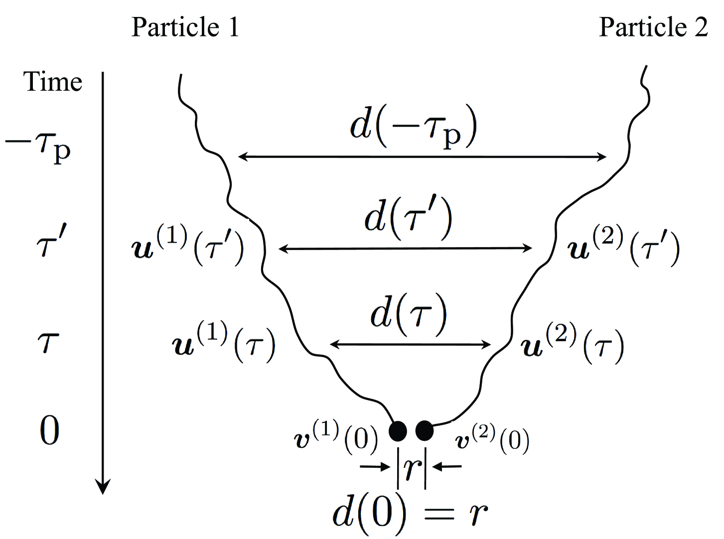
Figure 1.— Schematic figure illustrating the physical picture of the PP10 model for the relative velocity of two equal-size particles. At time 0, the separation of particles (1) and (2) is $r$. The velocity, ${\boldsymbol{v}}(0)$, of each particle at $t=0$, is determined by its memory of the flow velocity, ${\boldsymbol{u}}(\tau)$, along the particle trajectory in the past. The relative velocity of the two particles mainly depends on the flow velocity difference, ${\boldsymbol{u}}^{(2)}(\tau)-{\boldsymbol{u}}^{(1)}(\tau)$, they “saw” within about a friction timescale $\tau_{\rm p}$ in the past, i.e., $-\tau_{\rm p}\;\hbox to0.0pt{\lower 2.5pt\hbox{$\sim$}\hss}\raise 1.5pt\hbox{$<$}\;\tau\leq 0$. The flow velocity difference at a given time $\tau$ scales with the particle separation, $d(\tau)$. The particle separation satisfies the “initial” constraint $d(0)=r$ and increases backward in time. Due to particle inertia, a roughly ballistic separation is expected within a friction timescale. The trajectories plot here reflect a more-or-less linear separation of the two particles. The particle relative velocity also depends on the temporal correlation of the flow velocity differences the two particles “saw” at different times, say $\tau$ and $\tau^{\prime}$. The correlation timescale is associated with the turnover time of turbulent eddies encountered by the two particles.

Since the flow velocity difference scales with the distance, $S_{{\rm T}ij}$ has an indirect dependence on the particle separation at $\tau$ and $\tau^{\prime}$. We denote the particle separation at $\tau$ as ${\boldsymbol{d}}(\tau)$ ($\equiv{\boldsymbol{X}}^{(2)}(\tau)-{\boldsymbol{X}}^{(1)}(\tau)$). The vector ${\boldsymbol{d}}$ is stochastic because of the random dispersion of the particle pair by turbulent motions. $S_{{\rm T}ij}$ also has a dependence on the time lag $(\tau^{\prime}-\tau)$. This dependence is associated with the temporal correlation of turbulent structures or eddies encountered by the two particles between $\tau$ and $\tau^{\prime}$, and the correlation time is essentially the turnover time of these eddies. To estimate $S_{{\rm T}ij}$, we consider the (indirect) spatial dependence on the particle separation and the temporal dependence on the time lag separately.

We use a typical particle separation ${\boldsymbol{R}}(\tau,\tau^{\prime})$ between $\tau$ and $\tau^{\prime}$ to model the spatial dependence. Like ${\boldsymbol{d}}(\tau)$ and ${\boldsymbol{d}}(\tau^{\prime})$, ${\boldsymbol{R}}(\tau,\tau^{\prime})$ is also a random vector. We approximate the dependence on the separation by the Eulerian structure tensor of the flow velocity, $S_{ij}({\boldsymbol{R}})$, defined in eq. (7). We denote as $\Phi_{2}(\tau^{\prime}-\tau,R)$ the temporal correlation of the flow structure at the scale $R$. $\Phi_{2}$ is expected to be an even function of the time lag and is normalized to unity, $\Phi_{2}(0,R)=1$, at zero time lag. To distinguish from the temporal correlation, $\Phi_{1}(\tau^{\prime}-\tau)$, along the trajectory of a single particle (see §2), we have used a subscript “2” here for the two-particle case. The trajectory structure tensor is then modeled as the product of the two dependences (PP10),

$$S_{{\rm T}ij}({\boldsymbol{r}};\tau,\tau^{\prime})\simeq\big{\langle}S_{ij}({\boldsymbol{R}})\Phi_{2}\big{(}\tau^{\prime}-\tau,R\big{)}\big{\rangle}_{\boldsymbol{R}}$$ (16)

where $\langle\cdot\cdot\cdot\rangle_{\boldsymbol{R}}$ denotes the average over the statistics of the random vector, ${\boldsymbol{R}}$. This average is over the probability distributions of both the amplitude, $R$, and the direction of ${\boldsymbol{R}}$. Eq. (16) implicitly assumes the statistical independence of the velocity difference, $\Delta{\boldsymbol{u}}$, seen by the two particles from their separation, ${\boldsymbol{R}}$. Rigorously, the amplitudes of $\Delta{\boldsymbol{u}}$ and ${\boldsymbol{R}}$ may have a correlation. If the particle pair encounters an eddy with a larger velocity, the particle separation tends to be larger. For example, if $R$ is in the inertial range of the flow, $\Delta u\simeq\epsilon_{\rm R}^{1/3}R^{1/3}$ from the refined similarity hypothesis (Kolmogorov 1962), where $\epsilon_{\rm R}$ is the average dissipation rate over the scale $R$ seen by the particle pair. A positive correlation is expected between the fluctuations in $\epsilon_{\rm R}$ and $R$. Eq. (16) neglects this correlation and may underestimate $S_{{\rm T}ij}$ and hence the particle relative velocity.

The $\Phi_{2}$ term in eq. (16) does not depend on the direction of ${\boldsymbol{R}}$, so one can first take the angular average of $S_{ij}({\boldsymbol{R}})$ and then average the entire term over the PDF of the amplitude, $R$. The latter cannot be exactly performed because the PDF of $R$ is unknown. With some simple estimates, PP10 argued that simply using the rms of $R$ to evaluate $S_{{\rm T}ij}$ (instead of averaging over the PDF of $R$) only causes a small difference ($\simeq 10\%$) in the model prediction. Following PP10, we ignore the PDF of $R$ and insert the rms of $R$ to evaluate $S_{{\rm T}ij}$. For the simplicity of notation, we use $R$ to denote the rms particle distance in between $\tau$ and $\tau^{\prime}$ in the rest of the paper. A similar notation is adopted for $d(\tau)$ and $d(\tau^{\prime})$, which will denote the rms separations at $\tau$ and $\tau^{\prime}$, respectively. We approximate $R$ by the geometric average of $d(\tau)$ and $d(\tau^{\prime})$,

$$R(\tau,\tau^{\prime})=\left[d(\tau)d(\tau^{\prime})\right]^{1/2}.$$ (17)

The rms separation $d(\tau)$ as a function of time $\tau$ will be discussed in §3.2.3.

With the above assumptions, the trajectory structure tensor is modeled as,

$$S_{{\rm T}ij}({\boldsymbol{r}};\tau,\tau^{\prime})\simeq\big{\langle}S_{ij}({\boldsymbol{R}})\big{\rangle}_{\rm ang}\Phi_{2}\big{(}\tau^{\prime}-\tau,R\big{)}.$$ (18)

The angular average of $S_{ij}$ over the direction of ${\boldsymbol{R}}$ will be carried out in §3.2.2. In eq. (18), the dependence of $S_{{\rm T}ij}$ on ${\boldsymbol{r}}$ is through the dependence of $d(\tau)$, $d(\tau^{\prime})$ and $R$ on ${\boldsymbol{r}}$. We refer to $\boldsymbol{r}$ as the “initial” separation, although it actually corresponds to the current or final separation of the two particles. Our formulation indicates that the separation of particle pairs backward in time is crucial for the prediction of the particle relative speed.

Inserting eq. (18) into eq. (14) gives the PP10 model for the particle structure tensor,

$$S_{{\rm p}ij}({\boldsymbol{r}})=\int_{-\infty}^{0}\frac{d\tau}{\tau_{\rm p}}\int_{-\infty}^{0}\frac{d\tau^{\prime}}{\tau_{\rm p}}\big{\langle}S_{ij}({\boldsymbol{R}})\big{\rangle}_{\rm ang}\times\hskip 56.9055pt$$

$$\hskip 56.9055pt\Phi_{2}\big{(}\tau^{\prime}-\tau,R\big{)}\exp\left(\frac{\tau}{\tau_{\rm p}}\right)\exp\left(\frac{\tau^{\prime}}{\tau_{\rm p}}\right).$$ (19)

We will numerically compute this double integral after evaluating or modeling the angular average, the temporal correlation and the particle separation backward in time.

A simplification of the PP10 model is to set ${\boldsymbol{R}}$ to one of two distances, ${\boldsymbol{d}}(\tau)$ or ${\boldsymbol{d}}(\tau^{\prime})$, instead of their geometric average. We find that replacing ${\boldsymbol{R}}$ in eq. (19) by either ${\boldsymbol{d}}(\tau)$ or ${\boldsymbol{d}}(\tau^{\prime})$ leads to equivalent model prediction for the particle relative speed. This is because $\Phi_{2}$ in eq. (19) is an even function of $\Delta\tau$($\equiv\tau^{\prime}-\tau$), and the product of the two exponential cutoffs are invariant under the exchange of $\tau$ and $\tau^{\prime}$. If one sets ${\boldsymbol{R}}={\boldsymbol{d}}(\tau)$ in eq. (19), the integral over $\tau^{\prime}$ can be isolated, yielding,

$$S_{{\rm p}ij}=\frac{1}{\tau_{\rm p}}\int_{-\infty}^{0}\langle S_{ij}({\boldsymbol{d}}(\tau))\rangle_{\rm ang}F(\tau)\exp\left(\frac{\tau}{\tau_{\rm p}}\right)d\tau,$$ (20)

where the angular average is over the direction of ${\boldsymbol{d}}(\tau)$ and the function $F(\tau)$ is defined as,

$$F(\tau)=\frac{1}{\tau_{\rm p}}\int_{-\infty}^{0}\Phi_{2}\big{(}\tau^{\prime}-\tau,d(\tau)\big{)}\exp\left(\frac{\tau^{\prime}}{\tau_{\rm p}}\right)d\tau^{\prime}.$$ (21)

The factor $F(\tau)$ may be roughly viewed as a response function of the particle pair to turbulent eddies at the scale $d(\tau)$. Although not indicated explicitly, the factor $F(\tau)$ also depends on $r$ through its dependence on $d(\tau)$. We will refer to eqs. (20) and (21) as the simplified model. In the simplified model, $F(\tau)$ can be integrated analytically using assumed function forms of $\Phi_{2}$ in §3.2.1, and one only needs to numerically solve a single integral in eq. (20). On the other hand, for the original PP10 model, one must numerically evaluate the double integral in eq. (19).

3.2.1 The temporal correlation $\Phi_{2}$

To estimate the temporal correlation, $\Phi_{2}$, in the trajectory structure tensor, $S_{{\rm T}ij}$, we first consider a special case where the particle separation, $R$, is much larger than the integral length scale, $L$, of the flow. In this case, the flow velocities, ${\boldsymbol{u}}^{(1)}$ and ${\boldsymbol{u}}^{(2)}$, “seen” by the two particles are independent, and $S_{{\rm T}ij}$ can be written as $\langle u^{(1)}_{i}(\tau)u^{(1)}_{j}(\tau^{\prime})\rangle+\langle u^{(2)}_{i}(\tau)u^{(2)}_{j}(\tau^{\prime})\rangle$ (see eq. (9)). Both terms correspond to the trajectory correlation tensor $B_{{\rm T}ij}$ defined below eq. (3) in §2, and for identical particles the two terms are equal. Therefore, for $R\gg L$, $\Phi_{2}(\Delta\tau,R)$ is the same as the temporal correlation coefficient, $\Phi_{1}(\Delta\tau)$, along the trajectory of one particle.

In §2, we approximated $\Phi_{1}$ by the Lagrangian correlation function, $\Phi_{\rm L}$. Using the approximation again, we have $\Phi_{2}(\Delta\tau,\ell)=\Phi_{1}(\Delta\tau)\simeq\Phi_{\rm L}(\Delta\tau)$ for $\ell\gg L$. Two function forms, single- and bi-exponential, were adopted for $\Phi_{\rm L}$ in §2. With the single-exponential form, we set $\Phi_{2}(\Delta\tau,\ell)=\exp(-|\Delta\tau|/T_{\rm L})$ for $\ell\gg L$. An extension of this function to smaller scales gives,

$$\Phi_{2}(\Delta\tau,\ell)=\exp\left(-\frac{|\Delta\tau|}{T(\ell)}\right),$$ (22)

where $T(\ell)$ is essentially the correlation time or lifetime of turbulent eddies of size $\ell$. For $\ell\gg L$, we set $T(\ell)=T_{\rm L}$.

At smaller $\ell$, $T(\ell)$ can be estimated using the velocity scalings in the turbulent flow. For $\ell$ in the inertial range, we obtain $T(\ell)$ by dividing $\ell$ by the amplitude of the turbulent velocity fluctuations at this scale, which is $\left(S_{\rm ll}(\ell)+2S_{\rm nn}(\ell)\right)^{1/2}$. Using the Kolmogorov scaling for structure functions, we have $T(\ell)=C_{\rm T}\bar{\epsilon}^{-1/3}\ell^{2/3}$, where $C_{\rm T}=(11C_{\rm K}/3)^{-1/2}=0.52C_{\rm K}^{-1/2}$. The factor, $11/3$, is from the incompressibility relation $S_{\rm nn}=4S_{\rm ll}/3$ in the inertial range. Since the Kolmogorov constant $C_{\rm K}$ is $\simeq 2$, we set $C_{\rm T}\simeq 0.4$. A similar value of $C_{\rm T}$ was adopted by Zaichik & Alipchenkov (2003). In the viscous range with $\ell\ll\eta$, the flow velocity difference goes linearly with $\ell$, and $T({\ell})$ is expected to be constant. Lundgren (1981) predicted that $T(\ell)=\sqrt{5}\tau_{\eta}$ for $\ell\ll\eta$, which was later confirmed by numerical simulations of Girimaji & Pope (1990). We thus take $T(\ell)=\sqrt{5}\tau_{\eta}$ for $\ell\ll\eta$ in our model. We will use the bridging formula for $T(\ell)$ from Zaichik et al. (2006),

$$T(\ell)=T_{\rm L}\left[1-\exp\left(-\left(\frac{C_{\rm T}}{\sqrt{5}}\right)^{3/2}(\ell/\eta)\right)\right]^{-2/3}\times\hskip 28.45274pt$$

$$\hskip 76.82234pt\left[\frac{(\ell/\eta)^{4}}{(\ell/\eta)^{4}+(T_{\rm L}/(C_{\rm T}\tau_{\eta}))^{6}}\right]^{1/6},$$ (23)

which satisfies the scalings of $T(\ell)$ in different scale ranges.

One may also adopt a bi-exponential form for $\Phi_{2}(\Delta\tau,\ell)$ based on eq. (5) for the Lagrangian correlation function $\Phi_{\rm L}$ (see §2). Replacing $T_{\rm L}$ in eq. (5) by $T(\ell)$ gives,

$$\Phi_{2}(\Delta\tau,\ell)={\frac{1}{2\sqrt{1-2z^{2}}}}\bBigg@{3}\{\big{(}1+\sqrt{1-2z^{2}}\big{)}\times\hskip 142.26378pt$$

$$\hskip 25.6073pt\exp\Bigg{[}-\frac{2|\Delta\tau|}{\big{(}1+\sqrt{1-2z^{2}}\big{)}T(\ell)}\Bigg{]}-\big{(}1-\sqrt{1-2z^{2}}\big{)}\times$$

$$\exp\left[{-\frac{2|\Delta\tau|}{\big{(}1-\sqrt{1-2z^{2}}\big{)}T(\ell)}}\right]\bBigg@{3}\}.\hskip 36.98866pt$$ (24)

This bi-exponential form for $\Phi_{2}(\Delta\tau,\ell)$ was used in all the calculations in PP10. We will compute the predictions of the PP10 model using both the single- and bi-exponential correlation functions. We find the results from the two cases are close to each other, suggesting that the double integral in eq. (19) is insensitive to the function form of $\Phi_{2}(\Delta\tau,\ell)$. After the integration, the dependence on $\Phi_{2}(\Delta\tau,\ell)$ is essentially condensed to a dependence on the timescale $T(\ell)$. This is similar to the case of the one-particle velocity, which is insensitive to the form of $\Phi_{1}(\Delta\tau)$ (see §2). PP10 also considered the possible dependence of the parameter $z$ on the length scale $\ell$. It was found that including a reasonable length scale dependence of $z$ barely changes the model prediction. We will set $z$ to be constant in this study.

We next consider the simplified model represented by eqs. (20) and (21). With a single-exponential $\Phi_{2}$ (eq. (22)), the response factor $F(\tau)$ defined in eq. (21) can be integrated analytcally,

$$F(\tau)=\frac{T(d)}{T(d)-\tau_{\rm p}}\exp\left(\frac{\tau}{T(d)}\right)+\frac{2\tau_{\rm p}T(d)}{\tau_{\rm p}^{2}-T^{2}(d)}\exp\left(\frac{\tau}{\tau_{\rm p}}\right).$$ (25)

Since $\tau$ is negative, $F(\tau)$ is dominated by the first term if $T(d)\gg\tau_{\rm p}$, and it approaches $\exp\left(\tau/T(d)\right)$ in that limit. On the other hand, for $T(d)\ll\tau_{\rm p}$, the leading term is $\frac{2T(d)}{\tau_{\rm p}}\exp(\tau/\tau_{\rm p})$. Note that eq. (25) does not diverge at $T(d)=\tau_{\rm p}$. Applying the L’Hospital’s rule shows that it converges to $(\frac{1}{2}-\frac{\tau}{\tau_{\rm p}})\exp(\tau/\tau_{\rm p})$, as $T(d)\to\tau_{\rm p}$. Therefore, when numerically integrating eq. (20), we set $F(\tau)=(\frac{1}{2}-\frac{\tau}{\tau_{\rm p}})\exp(\tau/\tau_{\rm p})$ for $T(d)$ around $\tau_{\rm p}$.

With the bi-exponential temporal correlation, eq. (24), the response factor, $F(\tau)$, can also be integrated analytically. The integration is straightforward, but the resulting function for $F(\tau)$ is complicated and is thus omitted here. The predictions of the simplified model with single- and bi-exponential $\Phi_{2}(\Delta\tau,\ell)$ are also found to be close to each other.

3.2.2 Averaging over the direction of ${\boldsymbol{R}}$

We evaluate the angular average of $S_{ij}({\boldsymbol{R}})$ over the direction of ${\boldsymbol{R}}$. It follows from eq. (7) that $S_{ij}({\boldsymbol{R}})=S_{\rm nn}(R)\delta_{ij}+\left[S_{\rm ll}(R)-S_{\rm nn}(R)\right]R_{i}R_{j}/R^{2}$. The contraction of the tensor is $S_{ii}({\boldsymbol{R}})=S_{\rm ll}(R)+2S_{\rm nn}(R)$, which does not have a direct dependence on the direction of ${\boldsymbol{R}}$. Therefore, to predict the 3D rms relative speed, we do not need to perform the angular average. However, for the radial and tangential components, one must make an assumption for the direction of ${\boldsymbol{R}}$ and compute the angular average for the term $\propto R_{i}R_{j}/R^{2}$.

In PP10, we assumed that the direction of the separation change, $\Delta{\boldsymbol{R}}\equiv{\boldsymbol{R}}-{\boldsymbol{r}}$, caused by turbulent dispersion is completely random or isotropic. One can then insert ${\boldsymbol{R}}=\Delta{\boldsymbol{R}}+{\boldsymbol{r}}$ into $S_{ij}({\boldsymbol{R}})$ and take the average over the direction of $\Delta{\boldsymbol{R}}$. From the assumed isotropy of $\Delta{\boldsymbol{R}}$, we have $\langle r_{i}\Delta R_{j}\rangle=0$ and $\langle\Delta R_{i}\Delta R_{j}\rangle_{\rm ang}=\frac{1}{3}(R^{2}-r^{2})\delta_{ij}$, and hence $\langle R_{i}R_{j}\rangle_{\rm ang}\simeq r_{i}r_{j}+\frac{1}{3}(R^{2}-r^{2})\delta_{ij}$ (see PP10). The angular average $\langle S_{ij}({\boldsymbol{R}})\rangle_{\rm ang}$ is then given by,

$$\langle S_{ij}({\boldsymbol{R}})\rangle_{\rm ang}=\delta_{ij}\bigg{[}\left(\frac{1}{3}-\frac{r^{2}}{3R^{2}}\right)S_{\rm ll}(R)+\left(\frac{2}{3}+\frac{r^{2}}{3R^{2}}\right)\times\hskip 56.9055pt$$

$$\hskip 85.35826ptS_{\rm nn}(R)\bigg{]}+\Big{[}S_{\rm ll}(R)-S_{\rm nn}(R)\Big{]}\frac{r_{i}r_{j}}{R^{2}}.$$ (26)

The equation approaches $S_{ij}({\boldsymbol{r}})$ in the limit $R\to r$. PP10 showed that eq. (26) reproduces the S-T formula for the radial and tangential relative speeds. In the limit $R\gg r$, we have $\langle S_{ij}({\boldsymbol{R}})\rangle_{\rm ang}\simeq\frac{1}{3}\left[S_{\rm ll}(R)+2S_{\rm nn}(R)\right]$.

Here we make a simpler assumption than PP10: we take the direction of ${\boldsymbol{R}}$ (rather than $\Delta{\boldsymbol{R}}$) to be isotropic. This means $\langle R_{i}R_{j}/R^{2}\rangle_{\rm ang}=\frac{1}{3}\delta_{ij}$, and we have,

$$\langle S_{ij}({\boldsymbol{R}})\rangle_{\rm ang}=\frac{1}{3}\left[S_{\rm ll}(R)+2S_{\rm nn}(R)\right]\delta_{ij},$$ (27)

which suggests that the particle structure tensor $S_{{\rm p}ij}\propto\delta_{ij}$ (see eq. (19)), and hence $\langle w_{\rm r}^{2}\rangle=\langle w_{\rm t}^{2}\rangle$ (see eq. (10)) for particles of any size. A comparison of the two assumptions, eqs. (26) and (27), shows that they differ only at $R\;\hbox to0.0pt{\lower 2.5pt\hbox{$\sim$}\hss}\raise 1.5pt\hbox{$<$}\;r$.

As expected, the contraction $\langle S_{ii}(R)\rangle_{\rm ang}$ of both eq. (26) and eq. (27), is equal to $\left[S_{\rm ll}(R)+2S_{\rm nn}(R)\right]$, indicating that the two assumptions give the same prediction for the 3D rms relative velocity. The only difference between the two assumptions is the prediction for the radial and tangential components at $St\;\hbox to0.0pt{\lower 2.5pt\hbox{$\sim$}\hss}\raise 1.5pt\hbox{$<$}\;1$. In §3.2.4, we will compare the model predictions by the two assumptions. The angular average $\langle S_{ij}({\boldsymbol{d}})\rangle_{\rm ang}$ in the simplified model (eq. (20)) can be evaluated similarly, and the resulting expressions are in the same form as eqs. (26) and (27) with $d(\tau)$ replacing $R(\tau,\tau^{\prime})$.

3.2.3 The backward dispersion of particle pairs

We finally specify the (rms) particle separation, $d(\tau)$, as a function of $\tau$. The separation of inertial particle pairs backward in time has not been explored in the literature. Fortunately, Bec et al. (2010) carried out a detailed numerical study of the forward-in-time pair dispersion of inertial particles. Following PP10, we use their results to guide the assumption for the backward dispersion. We first consider the separation behavior of inertial-range particles with $\tau_{\eta}\;\hbox to0.0pt{\lower 2.5pt\hbox{$\sim$}\hss}\raise 1.5pt\hbox{$<$}\;\tau_{\rm p}\;\hbox to0.0pt{\lower 2.5pt\hbox{$\sim$}\hss}\raise 1.5pt\hbox{$<$}\;T_{\rm L}$.

Bec et al. (2010) found that the separation of inertial particles shows different behaviors at early and late times. At early times, a clear ballistic phase is observed for particles with $St\;\hbox to0.0pt{\lower 2.5pt\hbox{$\sim$}\hss}\raise 1.5pt\hbox{$>$}\;3$. In this phase, the separation increases linearly with time, and the phase lasts for about a friction timescale. The ballistic behavior is easy to understand: The particle velocity tends to be roughly constant for a memory timescale, $\tau_{\rm p}$. This also applies to the dispersion backward in time. We thus assume that, for particle pairs at an “initial” distance of $r$, the separation $d(\tau)$ in the time range $-\tau_{\rm p}\;\hbox to0.0pt{\lower 2.5pt\hbox{$\sim$}\hss}\raise 1.5pt\hbox{$<$}\;\tau\leq 0$ is given by,

$$d^{2}(\tau)=r^{2}+\langle w^{2}\rangle\tau^{2}$$ (28)

where $\langle w^{2}\rangle$ is the 3D variance of the particle relative velocity at time 0. The particle relative speed is actually what our model aims to predict. Therefore, the dependence of $d(\tau)$ on $\langle w^{2}\rangle$ in the ballistic phase leads to an implicit equation for $\langle w^{2}\rangle$(see §3.2.4).

Bec et al. (2010) also showed that, after a friction timescale, the dispersion of inertial-range particles make a transition to a tracer-like phase, where the separation variance increases as time cubed, a behavior known as the Richardson law. The Richardson law was first discovered for tracer pair dispersion at inertial-range scales. The transition to the Richardson phase at a friction timescale or so suggests the ballistic separation for a duration of $\tau_{\rm p}$ already brings the average particle distance into the inertial range of the flow. The Richardson behavior was observed in the tracer pair dispersion both forward and backward in time (Berg et al.  2006; see Appendix A). It is thus likely to exist also in the backward separation of inertial particles. We connect the Richardson phase to the ballistic phase at $\tau\simeq-\tau_{\rm p}$, and use the Richardson law

$$d^{2}(\tau)\simeq g\bar{\epsilon}|\tau|^{3}$$ (29)

at $\tau\;\hbox to0.0pt{\lower 2.5pt\hbox{$\sim$}\hss}\raise 1.5pt\hbox{$<$}\;-\tau_{\rm p}$, where $g$ is called the Richardson constant and $\bar{\epsilon}$ is the average dissipation rate of the flow. As the backward separation is typically faster than the forward case, the transition to the Richardson phase might occur slightly earlier than assumed here. Bec et al. (2010) did not report the value of $g$ in the Richardson phase of inertial particle pair dispersion. As in PP10, we will take $g$ as a parameter. In our model, we use a combined separation behavior that connects a ballistic and a Richardson phase at $\tau\simeq-\tau_{\rm p}$.

The Richardson behavior would end when the separation becomes larger than the integral length scale, $L$, of the turbulent flow. At such a large distance, the flow velocities “seen” by the two particles is uncorrelated, and the particle separation is expected to be diffusive like in a random walk. It is thus appropriate to switch the Richardson behavior to a diffusive phase with $d^{2}(\tau)\propto|\tau|$ at $d\;\hbox to0.0pt{\lower 2.5pt\hbox{$\sim$}\hss}\raise 1.5pt\hbox{$>$}\;L$. However, we find that the exact separation behavior at $d\gg L$ (or $R\gg L$) does not affect the prediction of our model. This is because at these scales both the structure functions, $S_{\rm ll}$ and $S_{\rm ll}$, and the timescale, $T(d)$ (or $T(R)$), become independent of $d$ (or $R$). Therefore, eq. (19) (or eq. (20)) is insensitive to the behavior of the separation once it becomes much larger than $L$. This is confirmed by the numerical solutions of eqs. (19) and (20). For convenience, we keep using the Richardson’s law even after $d$ exceeds $L$.

The separation behavior discussed above is based on the simulation results of Bec et al. (2010) for particles in the inertial range. For simplicity, we will use the same behavior for all particles, although its validity is questionable for small ($\tau_{\rm p}\;\hbox to0.0pt{\lower 2.5pt\hbox{$\sim$}\hss}\raise 1.5pt\hbox{$<$}\;\tau_{\eta}$) and large ($\tau_{\rm p}\;\hbox to0.0pt{\lower 2.5pt\hbox{$\sim$}\hss}\raise 1.5pt\hbox{$>$}\;T_{\rm L}$) particles. For small particles with $St\;\hbox to0.0pt{\lower 2.5pt\hbox{$\sim$}\hss}\raise 1.5pt\hbox{$<$}\;3$, a ballistic phase is not clearly observed in the $d^{2}$ vs. time plots in Fig. 5 of Bec et al. (2010). We expect that a short ballistic phase is likely to exist if one plots $(d^{2}-r^{2})$ (instead of $d^{2}$) vs. time (see Fig. 20 in Appendix A for the $(d^{2}-r^{2})$ vs. time plot for tracer particle pairs). However, for $St\;\hbox to0.0pt{\lower 2.5pt\hbox{$\sim$}\hss}\raise 1.5pt\hbox{$<$}\;3$ particles, the connection of the short ballistic phase to the Richardson behavior is more complicated than in the case of larger particles (Fig. 5 of Bec et al. 2010). This is because the pair separation of these particles does not enter the inertial range of the flow in a friction timescale or so. Therefore, an intermediate phase exists in between the ballistic and Richardson phases. Ideally, a three-phase behavior should be considered. Unfortunately, the separation behavior in the intermediate phase is completely unknown, and thus, to include it, one must adopt a pure parameterization. Here we take a simpler approximation: We still connect the Richardson behavior directly to the ballistic phase for $St\;\hbox to0.0pt{\lower 2.5pt\hbox{$\sim$}\hss}\raise 1.5pt\hbox{$<$}\;3$ particles, although it cannot be justified physically. Essentially, this parameterizes the later two phases by a single Richardson law with a free parameter $g$. Future numerical studies for the entire separation behavior of small particles is needed to improve the approximation. For the particle distance range, $\eta/4\;\hbox to0.0pt{\lower 2.5pt\hbox{$\sim$}\hss}\raise 1.5pt\hbox{$<$}\;r\;\hbox to0.0pt{\lower 2.5pt\hbox{$\sim$}\hss}\raise 1.5pt\hbox{$<$}\;\eta$, considered in our data analysis (see §6.1), our model with the assumed behavior does give acceptable prediction for $St\;\hbox to0.0pt{\lower 2.5pt\hbox{$\sim$}\hss}\raise 1.5pt\hbox{$<$}\;3$ particles. However, in the $r\to 0$ limit, a careful study of the intermediate separation phase of $St\;\hbox to0.0pt{\lower 2.5pt\hbox{$\sim$}\hss}\raise 1.5pt\hbox{$<$}\;3$ particles is necesary to accurately model their relative velocity.

The problem of using the assumed behavior for particles with $\tau_{\rm p}\gg T_{\rm L}$ is that the Richardson phase does not exit. The velocities of these large particles are uncorrelated even at small distances (§3.1). Therefore, at timescales larger than $\tau_{\rm p}$, the separation is likely diffusive, i.e., $d(\tau)\propto|\tau|$. Realistically, one needs to connect the ballistic phase to a diffusive behavior rather than a Richardson law at $|\tau|\sim\tau_{\rm p}$. However, it turns out that, at the end of the ballistic phase of these particles, the separation is already $\;\hbox to0.0pt{\lower 2.5pt\hbox{$\sim$}\hss}\raise 1.5pt\hbox{$>$}\;L$. As discussed earlier, once the separation exceeds $L$, the exact separation behavior would not significantly affect the model prediction. This justifies using a combined separation behavior with a ballistic and a Richardson phase also for $\tau_{\rm p}\gg T_{\rm L}$ particles.

So far, the initial distance, $r$, just provides a floor value in our assumption for the particle separation $d$ (eq. (28)). It is, however, possible that the value of $r$ has additional effects on the separation behavior. Bec et al. (2010) only explored $r$ above the Kolmogorov scale, and it is not clear whether the separation behavior has a qualitative difference if $r\;\hbox to0.0pt{\lower 2.5pt\hbox{$\sim$}\hss}\raise 1.5pt\hbox{$<$}\;\eta$. To model the particle collision speed, we are interested in the backward separation with $r\ll\eta$, and it would thus be helpful to systematically investigate whether and how the separation behavior changes as $r$ decreases below $\eta$. We defer such a study to a later work. Due to the uncertainty in the separation behavior for $r\ll\eta$, we will focus on testing the model prediction for the relative velocity at significant fractions of the Kolmogorov scale ($\eta/4\;\hbox to0.0pt{\lower 2.5pt\hbox{$\sim$}\hss}\raise 1.5pt\hbox{$<$}\;r\;\hbox to0.0pt{\lower 2.5pt\hbox{$\sim$}\hss}\raise 1.5pt\hbox{$<$}\;\eta$). We assume that the two-phase behavior discussed above applies for this range of $r$. Considering the existence of various uncertainties, the assumed separation behavior should be viewed more or less as a parameterization.

To constrain $g$ in the Richardson phase, in Appendix A we measure $g$ for the backward dispersion of tracer particle pairs in our simulated flow, which is used as a reference for inertial particles. The measured $g$ for tracers in our flow at a limited resolution shows a dependence on $r$, suggesting that the Richardson constant for inertial particles may also depend on $r$. When comparing our model prediction to the simulation results at different $r$, we will adjust $g$ to obtain best fits, and examine whether the best-fit values are consistent with the range of $g$ measured from tracer particles. The Richardson constant for inertial particles may also have a dependence on $\tau_{\rm p}$ (or $St$), which will be ignored for simplicity.

Finally, we point out that our model for the rms relative velocity does not directly account for the effect of the spatial clustering of the particles (see §7). Ideally, a theoretical model needs to consider the clustering and relative velocity statistics simultaneously. At a given time, the relative velocity determines the evolution of the spatial distribution of the particles, while the particle distribution may affect how the particles “see” the flow velocity and hence the evolution of the relative velocity statistics. However, modeling clustering and the relative velocity together self-consistently is very challenging, and is out of the scope of the current work.

3.2.4 Qualitative Behavior of Our Model Prediction

Our model for the particle structure tensor, $S_{{\rm p}ij}$, is now complete. Here we discuss the qualitative behavior of our model prediction. We start by considering the 3D variance, $\langle w^{2}\rangle$. The contraction of eq. (19) gives,

$${\displaystyle\langle w^{2}\rangle=\int_{-\infty}^{0}\frac{d\tau}{\tau_{\rm p}}\int_{-\infty}^{0}\frac{d\tau^{\prime}}{\tau_{\rm p}}\big{[}S_{\rm ll}(R)+2S_{\rm nn}(R)]\times}\hskip 28.45274pt$$

$$\hskip 56.9055pt{\displaystyle\Phi_{2}\big{(}\tau^{\prime}-\tau,R\big{)}\exp\left(\frac{\tau}{\tau_{\rm p}}\right)\exp\left(\frac{\tau^{\prime}}{\tau_{\rm p}}\right)},$$ (30)

which is an implicit equation of $\langle w^{2}\rangle$ because $R$ depends on $\langle w^{2}\rangle$ in the ballistic separation phase. In §6.1, we will solve the equation numerically using an iterative method.

The qualitative behavior of the model prediction for $\langle w^{2}\rangle$ can be obtained by analyzing the integrand in eq. (30). In the S-T limit ($\tau_{\rm p}\to 0$), the exponential cutoff terms, $\frac{1}{\tau_{\rm p}}\exp(\tau/\tau_{\rm p})$ and $\frac{1}{\tau_{\rm p}}\exp(\tau^{\prime}/\tau_{\rm p})$, in the integrand can be viewed as delta functions at $\tau=0$ and $\tau^{\prime}=0$, respectively. This suggests that $\langle w^{2}\rangle$ is approximately given by $\simeq(S_{\rm ll}+2S_{\rm nn})$ at $R(0,0)$. Since $R(0,0)=r$, we have $\langle w^{2}\rangle=\frac{\bar{\epsilon}}{3\nu}r^{2}$ for $r$ in the dissipation rate, which is consistent with the S-T prediction (see eq. (11)) for the 3D variance of the relative velocity.

The analysis of eq. (30) for larger particles is more complicated. We first note that $S_{\rm ll}(R)$, $S_{\rm nn}(R)$, and the timescale $T(R)$ in the correlation function $\Phi_{2}$ are all increasing functions of $R$. Since $R$ increases backward in time, the first factor in the integrand of eq. (30) increases with increasing $|\tau|$ and $|\tau^{\prime}|$. A larger $T(R)$ also tends to increase the integral because, with increasing $T(R)$, $\Phi_{2}$ allows contributions from a broader range of time lag ($\Delta\tau$). Together with the exponential cutoffs, these suggest that the contribution to the integral peaks at $\tau,\tau^{\prime}\simeq-\tau_{\rm p}$. We denote the particle separation at $\tau=\tau^{\prime}=-\tau_{\rm p}$ as $R_{\rm p}$ ($\equiv R(-\tau_{\rm p},-\tau_{\rm p})$), and refer to it as the primary distance.

In the extreme limit of large particles with $\tau_{\rm p}\gg T_{\rm L}$, $R_{\rm p}$ is expected to be much larger than the integral scale, $L$, of the flow. At $R_{\rm p}\gg L$, we have $S_{\rm ll}=S_{\rm nn}=2u^{\prime 2}$, and $T(R_{\rm p})=T_{\rm L}$. The exponential cutoff by $\Phi_{2}$ indicates that only the time pairs ($\tau$ and $\tau^{\prime}$) that satisfy the constraint $|\tau^{\prime}-\tau|\simeq T_{\rm L}$ give a significant contribution to the integral. Since $T_{\rm L}\ll\tau_{\rm p}$, $\Phi_{2}$ reduces the range of $\tau$ and $\tau^{\prime}$ that contributes to the double integral by a factor of $T_{\rm L}/\tau_{\rm p}$. Assuming the main contribution to the integral is from $R\simeq R_{\rm p}$ and accounting for the effect of $\Phi_{2}$, we find $\langle w^{2}\rangle\simeq 6u^{\prime 2}T_{\rm L}/\tau_{\rm p}$. This is consistent with eq. (12), meaning that our model correctly reproduces the large particle limit.

For inertial-range particles with $\tau_{\eta}\;\hbox to0.0pt{\lower 2.5pt\hbox{$\sim$}\hss}\raise 1.5pt\hbox{$<$}\;\tau_{\rm p}\;\hbox to0.0pt{\lower 2.5pt\hbox{$\sim$}\hss}\raise 1.5pt\hbox{$<$}\;T_{\rm L}$, the primary distance, $R_{\rm p}$, corresponds to inertial-range scales of the turbulent flow. Using the Kolmogorov scaling gives $S_{\rm ll},S_{\rm nn}\propto R_{\rm p}^{2/3}$ and $T(R_{\rm p})\propto R_{\rm p}^{2/3}$. From its definition, $R_{\rm p}$ is roughly the particle distance at the time when the ballistic phase connects to the Richardson phase (see §3.2.3). We thus assume that $R_{\rm p}$ is determined by a ballistic separation of duration $\tau_{\rm p}$, i.e., $R_{\rm p}\simeq\langle w^{2}\rangle^{1/2}\tau_{\rm p}$. The effect of $\Phi_{2}$ depends on how $T(R_{\rm p})$ compares to $\tau_{\rm p}$. If $T(R_{\rm p})>\tau_{\rm p}$, $\Phi_{2}\simeq 1$ for all time pairs in the range $-\tau_{\rm p}\;\hbox to0.0pt{\lower 2.5pt\hbox{$\sim$}\hss}\raise 1.5pt\hbox{$<$}\;\tau,\tau^{\prime}\;\hbox to0.0pt{\lower 2.5pt\hbox{$\sim$}\hss}\raise 1.5pt\hbox{$<$}\;0$. On the other hand, if $T(R_{\rm p})<\tau_{\rm p}$, $\Phi_{2}$ provides a factor of $T(R_{\rm p})/\tau_{\rm p}$, which follows from the same argument used above for the large particle limit. We find that both cases lead to the same scaling of $\langle w^{2}\rangle$ with $\tau_{\rm p}$. In the first case, eq. (30) is approximated by $\langle w^{2}\rangle\simeq[S_{\rm ll}(R_{\rm p})+S_{\rm nn}(R_{\rm p})]\propto R_{\rm p}^{2/3}$. With $R_{\rm p}\simeq\langle w^{2}\rangle^{1/2}\tau_{\rm p}$, we obtain $\langle w^{2}\rangle^{1/2}\propto\tau_{\rm p}^{1/2}$. In the second case with $T(R_{\rm p})<\tau_{\rm p}$, we include a factor of $T(R_{\rm p})/\tau_{\rm p}$ and estimate $\langle w^{2}\rangle$ as $\simeq[S_{\rm ll}(R_{\rm p})+S_{\rm nn}(R_{\rm p})]T(R_{\rm p})/\tau_{\rm p}\propto R_{\rm p}^{4/3}/\tau_{\rm p}$. It is straightforward to see that setting $R_{\rm p}\simeq\langle w^{2}\rangle^{1/2}\tau_{\rm p}$ in this estimate gives the same scaling, $\langle w^{2}\rangle^{1/2}\propto\tau_{\rm p}^{1/2}$, as the first case. Therefore, whether $T(R_{\rm p})$ is larger or smaller than $\tau_{\rm p}$, our model predicts a $\tau_{\rm p}^{1/2}$ (or $St^{1/2}$) scaling for inertial-range particles.

Using a similar argument, PP10 found that if the primary distance is determined by the Richardson’s law, $R_{\rm p}\simeq(g\bar{\epsilon}\tau_{p}^{3})^{1/2}$, the model also predicts a $St^{1/2}$ scaling for inertial-range particles. Since both the ballistic and Richardson behaviors yield a $St^{1/2}$ scaling, a combination of a ballistic and a Richardson phase produces the same scaling (PP10). The $St^{1/2}$ scaling has been previously predicted by models of Volk et al. (1980), Cuzzi and Hogan (2003), Ormel and Cuzzi (2007), and Zaichik & Alipchenkov (2003). As mentioned earlier, the scaling may also be obtained from a dimensional analysis under a scale-invariant assumption. If the dimensional analysis exactly holds, then the departure from the $St^{1/2}$ scaling for inertial-range particles in a simulation of limited resolution is caused completely by the effects from dissipation or driving scales. The derivation of the $St^{1/2}$ scaling in all the models assumes a sufficiently broad inertial range. The scaling would not exist if the Reynolds number of the turbulent flow is low. In fact, the predicted $St^{1/2}$ behavior has never been confirmed by simulations due to the low numerical resolution. PP10 showed that, to see the $St^{1/2}$ scaling, the Taylor Reynolds number of the turbulent flow must be larger than $\simeq 300$. This is higher than in the $512^{3}$ simulation used in the present study, and thus a clear $St^{1/2}$ scaling is not observed. It appears likely that the existence of this scaling can be verified at a twice larger resolution. We will conduct a $1024^{3}$ simulation in a future work.

The above analysis for the scaling behavior of $\langle w^{2}\rangle$ in different $St$ ranges can be similarly applied to the simplified model, eqs. (20) and (21). The prediction of the simplified model is qualitatively the same as the original PP10 model.

Finally, we examine the model prediction for the radial and tangential components of the relative velocity. The prediction for $\langle w_{\rm r}^{2}\rangle$ and $\langle w_{\rm t}^{2}\rangle$ depends on the angular average of $S_{{\rm T}ij}$ in eq. (19) (or eq. 20). In §3.3.2, we made two assumptions, eqs. (26) and (27), for the angular average. Inserting the first assumption, eq. (26), into eq. (19) and comparing it with eq. (10), we find,

$$\langle w_{\rm r}^{2}\rangle=\int_{-\infty}^{0}\frac{d\tau}{\tau_{\rm p}}\int_{-\infty}^{0}\frac{d\tau^{\prime}}{\tau_{\rm p}}\bigg{[}\left(\frac{1}{3}+\frac{2r^{2}}{3R^{2}}\right)S_{\rm ll}(R)+\hskip 56.9055pt$$

$$\hskip 28.45274pt\left(\frac{2}{3}-\frac{2r^{2}}{3R^{2}}\right)S_{\rm nn}(R)\bigg{]}\Phi_{2}\big{(}\tau^{\prime}-\tau,R\big{)}\exp\left(\frac{\tau+\tau^{\prime}}{\tau_{\rm p}}\right),$$

$$\langle w_{\rm t}^{2}\rangle=\int_{-\infty}^{0}\frac{d\tau}{\tau_{\rm p}}\int_{-\infty}^{0}\frac{d\tau^{\prime}}{\tau_{\rm p}}\bigg{[}\left(\frac{1}{3}-\frac{r^{2}}{3R^{2}}\right)S_{\rm ll}(R)+\hskip 56.9055pt$$

$$\hskip 28.45274pt\bigg{(}\frac{2}{3}+\frac{r^{2}}{3R^{2}}\bigg{)}S_{\rm nn}(R)\bigg{]}\Phi_{2}\big{(}\tau^{\prime}-\tau,R\big{)}\exp\left(\frac{\tau+\tau^{\prime}}{\tau_{\rm p}}\right).$$ (31)

In order to integrate these two equations, one needs to first solve eq. (30) for $\langle w^{2}\rangle$ due to the dependence of $R$ on $\langle w^{2}\rangle$ in the ballistic phase. It is easy to show that, in the limit $\tau_{\rm p}\to 0$, $R\to r$, and eq. (31) reduces to $\langle w_{\rm r}^{2}\rangle=S_{\rm ll}(r)$ and $\langle w_{\rm t}^{2}\rangle=S_{\rm nn}(r)$, reproducing the S-T formula, eq. (11). For larger particles with $\tau_{\rm p}\gg\tau_{\eta}$, we have $R_{\rm p}\gg r$, and thus eq. (31) predicts $\langle w_{\rm r}^{2}\rangle=\langle w_{\rm t}^{2}\rangle=\frac{1}{3}\langle w^{2}\rangle$, Therefore, like $\langle w^{2}\rangle$, both $\langle w_{\rm r}^{2}\rangle$ and $\langle w_{\rm t}^{2}\rangle$ scale as $St^{1/2}$ for inertial-range particles and as $St^{-1/2}$ in the large particle limit.

As discussed in §3.3.2, the second assumption, eq. (27), for the angular average of $S_{{\rm T}ij}$ predicts that $\langle w_{\rm r}^{2}\rangle=\langle w_{\rm t}^{2}\rangle=\frac{1}{3}\langle w^{2}\rangle$ for all particles. In the S-T limit, eq. (30) gives $\langle w^{2}\rangle=\frac{\bar{\epsilon}}{3\nu}r^{2}$, and thus $\langle w_{\rm r}^{2}\rangle=\langle w_{\rm t}^{2}\rangle=\frac{\bar{\epsilon}}{9\nu}r^{2}$. This means that the prediction by the second assumption for the radial and tangential relative speeds of $St\ll 1$ particles differs from the S-T formula, although it reproduces the S-T prediction for the 3D rms. We will test the model predictions for the relative velocity variances measured from our simulation data.

4. Statistics of the Simulated Flow

In this section, we describe the numerical method used in our simulation and discuss the statistical properties of the simulated flow. Our simulation was conducted in a periodic $512^{3}$ box with a length of $2\pi$ on each side. Using the Pencil code (Brandenburg & Dobler 2002, Johansen, Andersen, & Brandenburg 2004), we evolved the hydrodynamic equations,

$$\frac{\partial\rho}{\partial t}+\frac{\partial}{\partial x_{i}}\left(\rho u_{i}\right)=0,$$

$$\frac{\partial{u}_{i}}{\partial t}+{u_{j}}\frac{\partial{u_{i}}}{\partial x_{j}}=\frac{1}{\rho}\frac{\partial}{\partial x_{j}}\left[\rho\nu\left(\frac{\partial u_{i}}{\partial x_{j}}+\frac{\partial u_{j}}{\partial x_{i}}-\frac{2}{3}\delta_{ij}\frac{\partial u_{k}}{\partial x_{k}}\right)\right]\hskip 99.58464pt$$

$$-\frac{1}{\rho}\frac{\partial p}{\partial x_{i}}+{f_{i}},\hskip 48.36958pt$$ (32)

with an isothermal equation of state, $p=\rho C_{\rm s}^{2}$. The sound speed is set to unity, i.e., $C_{\rm s}=1$. The kinematic viscosity, $\nu$, is taken to be constant, $\nu=5\times 10^{-5}$. A large-scale force, $f_{i}$, generated in Fourier space using 20 modes in the wavenumber range of $1\leq k\leq 2$ is applied to drive and maintain the turbulent flow. The driving length scale, $L_{\rm f}$, is thus about 1/2 box size. The balance between the energy input by the driving force and the dissipation by viscosity leads to a statistical steady state with a 1D rms velocity, $u^{\prime}$, of 0.05, or a 3D rms of $0.085$. This weakly compressible flow is suitable for the application to turbulence in protoplanetary disks. At an rms Mach number of $0.085$, the flow statistics is essentially the same as incompressible turbulence (Padoan et al. 2004, Pan & Scannapieco 2011).

The integral length scale, $L$, in our simulated flow is found to be $\simeq 1$, i.e., about 1/6 box size. It is about 3 times smaller than the driving scale, $L_{\rm f}$. The integral scale, $L$, represents the (longitudinal) correlation length of the velocity field, and we computed it from the energy spectrum, $E(k)$, of the flow, using the relation $L=\frac{\pi}{2u^{\prime 2}}\int k^{-1}E(k)dk$ (Monin & Yaglom 1975). The energy spectrum, $E(k)$, is plot in the inset of Fig. (3). With $L=1$, the large-eddy turnover time is $T_{\rm eddy}=L/u^{\prime}=20$ in units in which the sound crossing time is $2\pi$.

The average energy dissipation rate per unit volume by the viscosity term is given by $\bar{\epsilon}=\frac{1}{2\bar{\rho}}\langle\rho\nu(\partial_{i}u_{j}+{\partial_{j}u_{i}}-\frac{2}{3}\delta_{ij}{\partial_{k}u_{k}})^{2}\rangle$, where $\bar{\rho}$ is the average density. In our weakly compressible flow, the density fluctuations and the velocity divergence can be neglected, and the dissipation rate can be estimated by $\bar{\epsilon}=\nu\langle\omega^{2}\rangle$, where $\langle\omega^{2}\rangle$ is the vorticity variance. We find that $\langle\omega^{2}\rangle=0.92$, implying that $\bar{\epsilon}\simeq 4.6\times 10^{-5}$. We also evaluated the dissipation rate from the 3rd-order longitudinal structure function using Kolmogorov’s 4/5 law, $\langle\Delta u_{\rm r}(\ell)^{3}\rangle=-\frac{4}{5}\bar{\epsilon}\ell$, for $\ell$ in the inertial range. This latter method gives a larger dissipation rate, $\bar{\epsilon}=5\times 10^{-5}$, suggesting that a small fraction, $\simeq 8\%$, of kinetic energy is dissipated by numerical diffusion. The effective viscosity is thus larger than the adopted value by the same amount. We take the effective viscosity to be $5.4\times 10^{-5}$ and use it in our estimates of the Kolmogorov scales. We compute the Kolmogorov timescale from the vorticity variance as $\tau_{\eta}=\langle w^{2}\rangle^{-1/2}=1.04$. The Kolmogorov length scale is estimated to be $\eta=(\nu^{3}/\bar{\epsilon})^{1/4}=0.0075$, which corresponds to $\simeq 0.6$ cell size of the computation grid. The Kolmogorov velocity scale is $u_{\eta}=(\nu\bar{\epsilon})^{1/4}=0.0072$ in units of the sound speed.

The Reynolds number of our simulated flow is $Re\equiv u^{\prime}L/\nu\simeq 1000$. A more commonly-used Reynolds number in turbulence studies is the Taylor Reynolds number, $Re_{\lambda}\equiv u^{\prime}\lambda/\nu$, where the Taylor micro length scale is defined as $\lambda\equiv(15u^{\prime 2}/\langle\omega^{2}\rangle)^{1/2}$. We find that $\lambda=0.2$ in our simulated flow, and thus $Re_{\lambda}\simeq 200$. From the definitions of $u_{\eta}$ and $Re_{\lambda}$, we have $u^{\prime}/u_{\eta}=(Re_{\lambda}/\sqrt{15})^{1/2}$.

4.1. The Lagrangian Correlation Function and the Timescales

To study the Lagrangian statistics, we integrated the trajectories of $33.6$ million tracer particles with zero inertia in the simulated flow. The total number of tracer particles corresponds to an average number density of 1 particle per 4 computational cells. To obtain the particle velocity inside a cell, we selected the triangular-shaped-cloud interpolation method already implemented in the Pencil code (Johansen and Youdin 2007). We output the particle positions to a data file in each $0.1\tau_{\eta}$. The Lagrangian correlation function, $\Phi_{\rm L}(\Delta\tau)$, is computed as the average of the velocity correlation, $\langle u_{i}({\boldsymbol{X}}(t),t)u_{i}({\boldsymbol{X}}(t+\Delta\tau),t+\Delta\tau)\rangle/3u^{\prime 2}$, along the trajectories, ${\boldsymbol{X}}(t)$, of all particles. We considered both positive and negative $\Delta\tau$, corresponding to Lagrangian trajectories forward and backward in time, respectively. Our data confirmed that $\Phi_{\rm L}$ is an even function of $\Delta\tau$, as expected from statistical stationarity (see §2). We find that the Lagrangian correlation timescale, $T_{\rm L}$ ($\equiv\int\Phi_{\rm L}(\Delta\tau)d\Delta\tau$), is $\simeq 15$, which is about 0.75 eddy turnover time, $T_{\rm eddy}$. This is consistent with the simulation result of Yeung et al. (2006). Since $\tau_{\eta}=1.04$ in our flow, we have $T_{\rm L}=14.4\tau_{\eta}$.

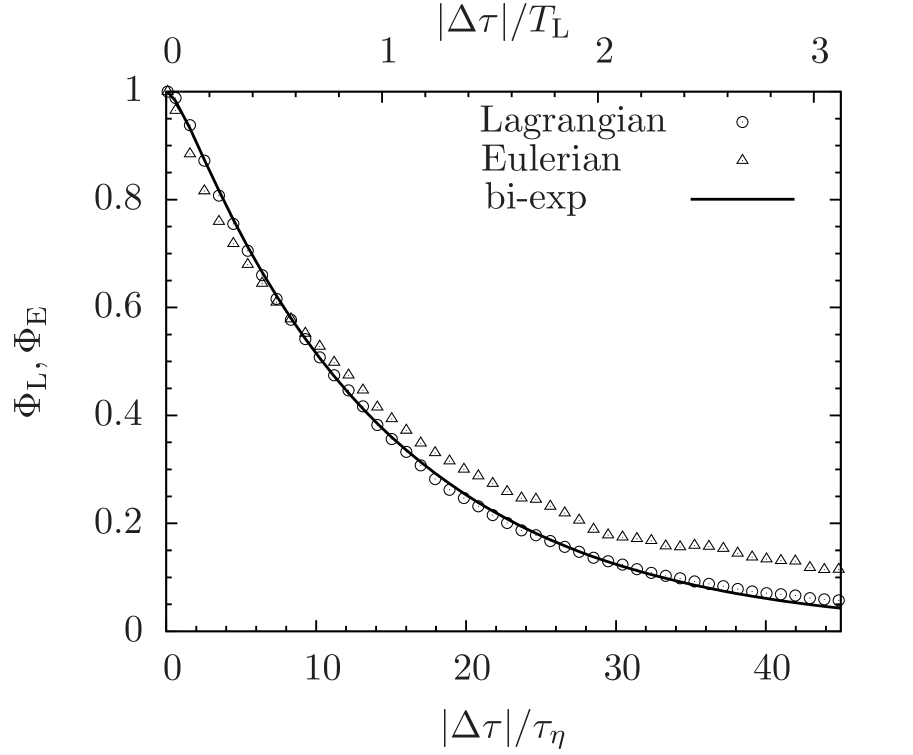
Figure 2.— Lagrangian ($\Phi_{\rm L}$; circles) and Eulerian ($\Phi_{\rm E}$; triangles) temporal correlation functions in our simulated flow. The time lag, $\Delta\tau$, is normalized to the Kolmogorov timescale, $\tau_{\eta}$ and the Lagrangian correlation time, $T_{\rm L}$, on the bottom and top X-axises, respectively. The solid line shows the best fit for $\Phi_{\rm L}$ using the bi-exponential function, eq. (5).

The Lagrangian correlation, $\Phi_{\rm L}$, in our flow is plot as circles in Fig.  2, where the time lag, $|\Delta\tau|$, is normalized to the Kolmogorov timescale, $\tau_{\eta}$ and the Lagrangian correlation time, $T_{\rm L}$, on the bottom and top X-axises, respectively. The solid line shows the bi-exponential function, eq. (5), given in §2. The parameter $z$ is set to 0.3, which suggests that the Taylor micro timescale, $\tau_{\rm T}$, is $\simeq 4.3\tau_{\eta}$. This value of $\tau_{\rm T}$ corresponds to an acceleration variance, $a^{2}\simeq 5.2(u_{\eta}/\tau_{\eta})^{2}$. The bi-exponential function matches very well the simulation data. On the other hand, we find that a single exponential function could not give a satisfactory fit to $\Phi_{\rm L}$.

We also considered the Eulerian temporal correlation function, $\Phi_{\rm E}(\Delta\tau)$. It is computed as the average, $\langle u_{i}({\boldsymbol{x}},t)u_{i}({\boldsymbol{x}},t+\Delta\tau)\rangle/3u^{\prime 2}$, over all grid points ${\boldsymbol{x}}$. The result is plot as triangles in Fig. 2. $\Phi_{\rm E}$ is smaller than the Lagrangian correlation $\Phi_{\rm L}$ at small time lags, and then becomes larger at $|\Delta\tau|\;\hbox to0.0pt{\lower 2.5pt\hbox{$\sim$}\hss}\raise 1.5pt\hbox{$>$}\;8\tau_{\eta}\simeq 0.55T_{\rm L}$. Due to the slower decrease of $\Phi_{\rm E}$ at large time lags, the Eulerian correlation time, $T_{\rm E}\equiv\int\Phi_{\rm E}(\Delta\tau)d\Delta\tau$, is slightly (10%) larger than $T_{\rm L}$. We find that $T_{\rm E}=15.9\tau_{\eta}$. The Eulerian correlation function is of interest for large inertial particles with $\tau_{\rm p}\gg T_{\rm L}$. Due to their large inertia, these particles have small velocities and thus may stay around as the flow sweeps by. Therefore, unlike small particles, the temporal series of the flow velocity “seen” by the large particles may be better described by the Eulerian velocity. This suggests that, for $\tau_{\rm p}\;\hbox to0.0pt{\lower 2.5pt\hbox{$\sim$}\hss}\raise 1.5pt\hbox{$>$}\;T_{\rm L}$, it may be appropriate to replace the Lagrangian correlation used in our model by the Eulerian correlation. However, the Eulerian correlation function and timescale are quite close to the Lagrangian ones, and using the Lagrangian correlation for all particles in our model gives satisfactory predictions for both the 1-particle velocity and the 2-particle relative velocity at any $St$ (§5 and §6.1).

We summarize the relevant timescales in the simulated flow and list them in an increasing order. The smallest timescale is Kolmogorov time $\tau_{\eta}$, and we use it as a reference timescale. The Taylor micro scale, $\tau_{\rm T}$, was found to be $4.3\tau_{\eta}$ from the bi-exponential fit to the Lagrangian correlation function. The next timescale is the Lagrangian correlation time, $T_{\rm L}$, which is $14.4\tau_{\eta}$. The Eulerian correlation time is slightly larger, $T_{\rm E}\simeq 15.9\tau_{\eta}$. The large eddy turnover time, $T_{\rm eddy}$, was measured to be $\simeq 19.2\tau_{\eta}$. Another commonly-used timescale is the dynamical time, $\tau_{\rm dyn}$, defined as the forcing length scale, $L_{\rm f}$, divided by the 3D rms velocity ($\sqrt{3}u^{\prime}$). We find that $\tau_{\rm dyn}=35\tau_{\eta}$.

In this work, we will express the particle friction time primarily by $St$ and $\Omega$. They correspond to normalizations to $\tau_{\eta}$ and $T_{\rm L}$, which are convenient for small and large particles, respectively. One may also normalize $\tau_{\rm p}$ to the large eddy turnover time, and define $\Omega_{\rm eddy}=\tau_{\rm p}/T_{\rm eddy}$, which may be more convenient for practical applications. However, we prefer using $\Omega$ than $\Omega_{\rm eddy}$, because, according to our model, it is $T_{\rm L}$ that directly enters the physics of turbulence-induced particle velocity. Using the measured values of the timescales in our simulation, one may convert the normalizations by $\Omega_{\rm eddy}=0.75\Omega=0.052St$.

4.2. The Flow Structure Functions and Energy Spectrum

In Fig. 3, we show the longitudinal ($S_{\rm ll}$; open circles) and transverse ($S_{\rm nn}$; filled circles) structure functions in our simulated flow. The structure functions are measured from the velocity differences along the 3 directions, ${\boldsymbol{e}}_{1}$, ${\boldsymbol{e}}_{2}$ and ${\boldsymbol{e}}_{3}$, of the simulation grid. For $S_{\rm ll}(\ell)$, we computed and averaged the variances of $\Delta u_{11}(\ell)$($\equiv u_{1}({\boldsymbol{x}}+\ell{\boldsymbol{e}}_{1})-u_{1}({\boldsymbol{x}})$), $\Delta u_{22}(\ell)$ and $\Delta u_{33}(\ell)$ over all the points, ${\boldsymbol{x}}$. Similarly, $S_{\rm nn}(\ell)$ is obtained by averaging the variances of $\Delta u_{12}(\ell)$($\equiv u_{1}({\boldsymbol{x}}+\ell{\boldsymbol{e}}_{2})-u_{1}({\boldsymbol{x}})$), $\Delta u_{13}(\ell)$, $\Delta u_{21}(\ell)$, $\Delta u_{23}(\ell)$, $\Delta u_{31}(\ell)$ and $\Delta u_{32}(\ell)$.

As discussed earlier, Kolmogorov’s similarity theory predicts that $S_{\rm ll}(\ell)\simeq C_{\rm K}(\bar{\epsilon}\ell)^{2/3}$ for $\ell$ in the inertial range. We thus compensated the structure functions by $(\bar{\epsilon}\ell)^{2/3}$ in Fig. 3. A limited inertial range is seen in both $S_{\rm ll}$ and $S_{\rm nn}$. The Kolmogorov constant $C_{\rm K}$ is about 2. In the inertial range, the scaling exponent for $S_{\rm ll}$ is found to be slightly larger than 2/3, while the slope of $S_{\rm nn}$ is close to 2/3. The ratio of the two structure functions in the inertial range is about 1.25, slightly smaller than the value, 4/3, expected from the incompressibility condition (see §3). This is perhaps because our flow is weakly compressible. Another possibililty is that the inertial range is too short to allow an accurate measurement of this ratio. Both structure functions become smooth, i.e., $\propto\ell^{2}$, as $\ell$ decreases toward the Kolmogorov scale, and approach $2u^{\prime 2}$ in the limit $\ell\gg L$ (§3).

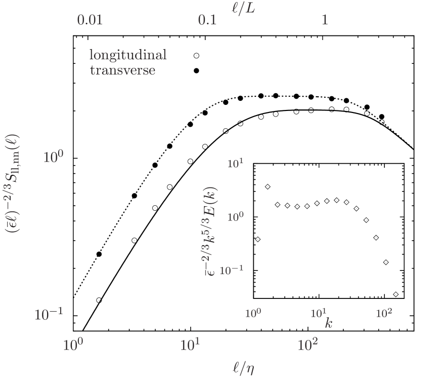
Figure 3.— Longitudinal (open circles) and transverse (filled circles) structure functions in our simulated flow. The structure functions are compensated by the Kolmogorov scaling in the inertial range. The solid and dashed lines are fitting functions, eqs. (8) and (33), for $S_{\rm ll}$ and $S_{\rm nn}$, respectively. The bottom and top X-axises normalize $\ell$ to the Kolmogorov scale and the integral scale, respectively. The inset shows the energy spectrum of the flow, compensated by $\bar{\epsilon}^{2/3}k^{-5/3}$.

The solid line in Fig. 3 is the connecting formula, eq. (8), for $S_{\rm ll}$ (§3). We set $C_{\rm K}=2$ in the formula. The line gives a fairly good fit to the data points. As discussed in §3, with the connecting formula for $S_{\rm ll}$, one may obtain a fitting function for $S_{\rm nn}$ using the incompressibility relation $S_{\rm nn}=S_{\rm ll}+\frac{1}{2}\ell dS_{\rm ll}/d\ell$. However, the fitting function obtained this way overestimates $S_{\rm nn}$ in the inertial range, perhaps because the incompressibility condition does not exactly hold in our flow (see above). For a more accurate fit, we adopted a separate connecting formula for $S_{\rm nn}$,

$$S_{\rm nn}=2u^{\prime 2}\left[1-\exp\left(-\frac{(\ell/\eta)^{4/3}}{(15C_{\rm Kn}/2)}\right)\right]\times\hskip 56.9055pt$$

$$\hskip 56.9055pt\left[\frac{(\ell/\eta)^{4}}{(\ell/\eta)^{4}+(2u^{\prime 2}/C_{\rm Kn}u_{\eta}^{2})^{6}}\right]^{1/6},$$ (33)

where $C_{\rm Kn}$ is the scaling coefficient for $S_{\rm nn}$ in the inertial range. This connecting formula correctly reproduces the scaling behaviors of $S_{\rm nn}$ in different scale ranges. Its form is slightly different from eq. (8) for $S_{\rm ll}$. The dotted line in Fig. 3 corresponds to eq. (33) with $C_{\rm Kn}\simeq 1.25C_{\rm K}=2.5$. We will use eqs. (8) and (33) in the computation of our model prediction for the particle relative velocity.

The inset of Fig. 3 show the energy spectrum, $E(k)$, of our flow. The Kolmogorov theory predicts $E(k)=K{\bar{\epsilon}}^{2/3}k^{-5/3}$ in the inertial range, and we compensated the spectrum by $\bar{\epsilon}^{2/3}k^{-5/3}$. The power-law range ($3\leq k\leq 10$) in the spectrum appears to be shorter than in the structure functions. The constant $K$ is measured to be $\simeq 1.7$, consistent with previous studies (Ishihara et al. 2009). It is also consistent with the relation $K=0.76C_{\rm K}$ (Monin & Yaglon 1975), as the Kolmogorov constant, $C_{\rm K}$, for $S_{\rm ll}$ was found to be $\simeq 2$.

5. One-particle Root-mean-square Velocity

In our simulation, we included 14 species of inertial particles of different sizes. The friction timescale of the particles spans about four decades from $\simeq 0.1\tau_{\eta}$ to $\simeq 41T_{\rm eddy}$ ($\simeq 54T_{\rm L}$ or $\simeq 800\tau_{\eta}$), covering the entire scale range of the simulated flow. The friction timescale is equally spaced, increasing by a factor of two in each successive species. The number of particles contained in each species is 33.6 million, corresponding to an average particle density of one per 4 computational cells. The same number of tracer particles was included to study the Lagrangian statistics (§4.1). The integration of the particle trajectories is computationally very expensive. Using 4096 cores (512 Harpertown nodes) on the NASA/Ames Pleiades supercomputer, the simulation was run for 14 days, corresponding to a total CPU cost of 1.4 million hours.

To evolve the particle equation of motion (eq. 1), we adopted the triangular-shaped-cloud (TSC) method to interpolate the flow velocity inside the computational cells. The TSC interpolation is a well-established method (Hockney & Eastwood 1981, Johansen & Youdin 2007) that makes use of the nearest 27 grid points in a 3D simulation. In 1D, the weighting factor for the nearest 3 grid points is set to be quadratic with the distance to the points. The velocity difference in our simulated flow is linear with $\ell$ around and below the cell size, $\Delta x$, as seen from the $\ell^{2}$ scaling of the structure functions toward $\Delta x$ (bottom data points) in Fig. 3. This implies that the subgrid velocity field can be well approximated by a linear interpolation (Pan et al. 2011). The linear scaling is also captured by the TSC method. It is straightforward to show that, if the flow velocity is already linear around the resolution scale (approximately the case in our simulated flow), the scaling of the interpolated velocity at subgrid scales by the TSC method would be exactly linear, as the quadratic terms in the weighting functions cancel out in this special case. In comparison to the linear interpolation, the TSC method is of higher order and has the advantage of smoother connections at cell boundaries.

Initially, the 33.6 million particles in each species are distributed randomly in the simulation box. Each component of the initial particle velocity is also random, independently drawn from a uniform distribution in the range [-0.01, 0.01]. Therefore, the initial (1D) rms, $v^{\prime}(0)$, of each velocity component of all the particles is $0.01/\sqrt{3}$, equivalent to a 3D rms of 0.01. The numerical values given here are in units of the gas sound speed, which was set to unity in the simulation. The initial particle conditions for all the 14 species are the same. We evolved the turbulent flow and the particle trajectories together right from the beginning of the simulation. At time zero, the gas velocity and density are set to zero and unity, respectively.

Our simulation run lasted for about $26T_{\rm eddy}$ (or $35T_{\rm L}$), and we saved 52 snapshots with an equal separation of $0.5T_{\rm eddy}$. The black dotted line in Fig. 4 is the 3D rms of the flow velocity ($\sqrt{3}u^{\prime}$) as a function of time, which shows that the flow is fully developed and reaches a (quasi) steady state at $t_{\rm dev}\simeq 5-10T_{\rm eddy}$. From top to bottom, the colored lines in Fig. 4 plot the 3D rms velocities of inertial particles with $St(\Omega)[\Omega_{\rm eddy}]=0.39(0.027)[0.02]$, $6.21(0.41)[0.32]$, $12.4(0.84)[0.65]$, $24.9(1.7)[1.3]$, $49.7(3.4)[2.6]$, $99.4(6.8)[5.2]$, $199(13.5)[10.4]$, $398(27)[20.7]$, and 795(54)[41.4], respectively. The numbers in the parentheses and square brackets correspond to $\Omega$ and $\Omega_{\rm eddy}$, respectively. We find there are dips at earlier times in the curves for relatively large particles. When our first snapshot was saved at $0.5T_{\rm eddy}$, particles with $\tau_{\rm p}\;\hbox to0.0pt{\lower 2.5pt\hbox{$\sim$}\hss}\raise 1.5pt\hbox{$>$}\;0.5T_{\rm eddy}$ partially lost the memory of the initial rms velocity, and meanwhile their velocity had some contribution from the flow velocity, $u^{\prime}$, between $t=0$ and $0.5T_{\rm eddy}$. However, since $u^{\prime}$ was 0 at $t=0$, this contribution turns out to be small and does not compensate the decrease due to the memory loss of the initial velocity. This causes a decrease in $v^{\prime}$ and leads to dips at $t\;\hbox to0.0pt{\lower 2.5pt\hbox{$\sim$}\hss}\raise 1.5pt\hbox{$>$}\;0.5T_{\rm eddy}$. Due to their short memory time, the small particles forgot their initial velocity, $v^{\prime}(0)$, at the first snapshot, and their velocity was close to the flow velocity at $0.5T_{\rm eddy}$, which is already slightly larger than $v^{\prime}(0)$. Therefore, no dips appear for the small particles with $\tau_{\rm p}\;\hbox to0.0pt{\lower 2.5pt\hbox{$\sim$}\hss}\raise 1.5pt\hbox{$<$}\;0.5T_{\rm eddy}$. The top six color lines appear to reach a steady state at $\simeq 10T_{\rm eddy}$. For the bottom three lines, $v^{\prime}(t)$ keeps increasing gradually but almost monotonically. This may imply that these largest particles need more time to relax. It is also possible that the slow increase of $v^{\prime}$ at late times is simply caused by the slight rise of the flow velocity (see the black dotted line).

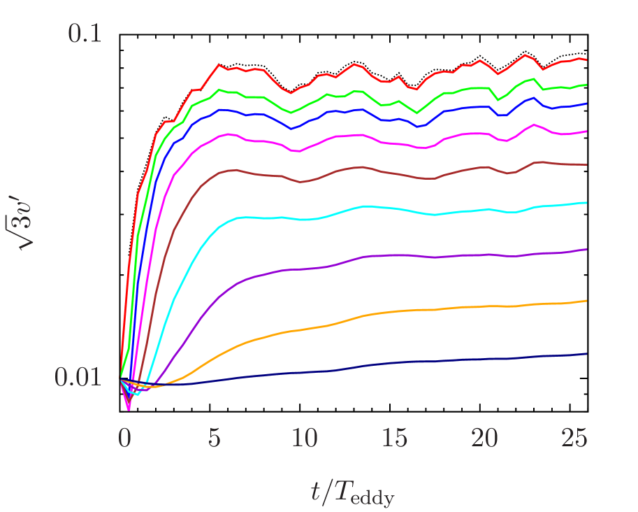
Figure 4.— The temporal evolution of the 3D rms velocity, $\sqrt{3}v^{\prime}$, of inertial particles of different sizes. The thin dotted line shows the 3D rms flow velocity, which reaches a (quasi) steady state at $t\;\hbox to0.0pt{\lower 2.5pt\hbox{$\sim$}\hss}\raise 1.5pt\hbox{$>$}\;5-10T_{\rm eddy}$. The flow rms velocity is 0 at time zero, and the dotted line starts from $0.5T_{\rm eddy}$ when the first snapshot is saved. From top to bottom, the color lines correspond to the rms velocity for particles with $St=0.39$, 6.12, 12.4, 24.9, 49.7, 99.4, 199, 398 and 795, respectively. The velocity is in units of the sound speed of the flow, which is set to unity in the simulation.

The relaxation timescale for inertial particles in a stationary turbulent flow is essentially the time for the particles to forget the initial condition, and is roughly given by the friction timescale, if the initial velocity is not much larger than the final steady-state value (as is the case for our initial conditions). The estimate for the relaxation time in our simulation is a little complicated because the particles are released to the flow before $t_{\rm dev}$. For particles with $\tau_{\rm p}\ll t_{\rm dev}$, the dynamical relaxation is expected once the flow is fully developed, i.e., at $\simeq t_{\rm dev}$. This is the case for the top 5-6 color lines in Fig. 4.

For the bottom 3-4 lines, $\tau_{\rm p}\;\hbox to0.0pt{\lower 2.5pt\hbox{$\sim$}\hss}\raise 1.5pt\hbox{$>$}\;t_{\rm dev}$, and we expect these particles would be relaxed at some time in the range ($\tau_{\rm p}$, $t_{\rm dev}+\tau_{\rm p}$). The lower limit is the minimum relaxation time, and the upper limit is based on the consideration that, if the particle evolution started at $t_{\rm dev}$ instead of time 0, the particles would relax at $\simeq t_{\rm dev}+\tau_{\rm p}$. From this estimate, the third largest particles ($St=199$) are relaxed by $\;\hbox to0.0pt{\lower 2.5pt\hbox{$\sim$}\hss}\raise 1.5pt\hbox{$<$}\;20T_{\rm eddy}$, and the second largest ones ($St=398$) are likely relaxed by the end of the simulation. On the other hand, the largest ($St=795$) particles may not have reached a relaxed state. However, the quite flat $v^{\prime}(t)$ of the $St=795$ particles indicates the possibility they are actually relaxed toward the end of the simulation. If that is the case, a likely reason for it is that the chosen initial condition (e.g., the rms velocity) happens to be very similar to the expected relaxed state of these particles. This similarity may reduce the relaxation time. We assume that all particles in our simulation are relaxed in the last 5-6 $T_{\rm eddy}$.

In our data analysis, we average over three snapshots at $t=21.5$, 24 and $26T_{\rm eddy}$. For the uniformity of the data sample, we use the same snapshots for all particle species. Since the largest particles become relaxed around the end of the simulation, we only select late snapshots at $t\;\hbox to0.0pt{\lower 2.5pt\hbox{$\sim$}\hss}\raise 1.5pt\hbox{$>$}\;20T_{\rm eddy}$. The purpose of averaging over a number of snapshots is to obtain better statistics by increasing the sample size. It is thus helpful to use well-separated snapshots with independent statistics. A temporal separation of $\simeq 2T_{\rm eddy}$ guarantees the particle velocities at the selected snapshots are independent for the first 10 particle species. The velocities of the largest four particles remain correlated for significantly longer than $\simeq 2T_{\rm eddy}$. Therefore, unlike the case of smaller particles, using the selected snapshots may not effectively increase the independent sample size or the measurement accuracy. If the computation resources allow, it would be ideal to run the simulation much longer and collect snapshots separated by a few friction times of the largest particles.

In Fig. 5, we show the simulation result for the 1D rms, $v^{\prime}$, of the particle velocity as a function of $St$. We normalized $v^{\prime}$ by the rms velocity, $u^{\prime}$, of the flow. The top X-axis normalizes the friction time to the Lagrangian correlation time. One may convert $St$ (or $\Omega$) to $\Omega_{\rm eddy}$ by $\Omega_{\rm eddy}=0.052St$ (or $\Omega_{\rm eddy}=0.75\Omega)$. The dotted and solid lines are predictions, eq. (4) and eq. (6), of our model using single- and bi-exponential forms for the temporal correlation function, respectively. The model approximates the trajectory correlation function, $\Phi_{1}$, by the Lagrangian correlation function, $\Phi_{\rm L}$ (see §2). For the bi-exponential case, we set the parameter $z=0.3$, which best fits $\Phi_{\rm L}$ measured from the Lagrangian trajectories (see §4.1). The two lines almost coincide, indicating that the model prediction for $v^{\prime}$ is insensitive to the exact form of the correlation function, and depends only on the correlation timescale. In both curves, we set $T_{\rm L}=15.4\tau_{\eta}$, generally consistent with the directly measured value of $14.4\tau_{\eta}$ (see §4.1). As expected, $v^{\prime}$ follows the $St^{-1/2}$ scaling (the dotted line segment) at $\Omega\gg 1$. This supports our claim that the largest particles are dynamically relaxed at the end of the run.

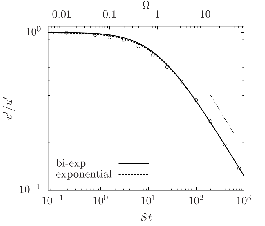
Figure 5.— The 1-particle rms velocity, $v^{\prime}$, as a function of the particle friction time. The bottom and top X-axises normalize $\tau_{\rm p}$ to $\tau_{\eta}$ and $T_{\rm L}$, respectively. The dotted and solid lines are the predictions, eq. (4) and eq. (6), of our model using single- and bi- exponential forms for the temporal correlation function, respectively. In both cases, $T_{\rm L}$ is set to $15.4\tau_{\eta}$, and the parameter $z$ in the bi-exponential case is set to 0.3. The thin dotted line segment denotes a $St^{-1/2}$ scaling.

The flow velocity “seen” by large particles with $\tau_{\rm p}\;\hbox to0.0pt{\lower 2.5pt\hbox{$\sim$}\hss}\raise 1.5pt\hbox{$>$}\;T_{\rm L}$ may be closer to Eulerian than Lagrangian (§4.1), and thus using $\Phi_{\rm L}$ for the trajectory correlation $\Phi_{1}$ is not well justified (§2). However, the assumption is validated by our simulation result for all particles. This is because, first, based on our model prediction, $v^{\prime}$ is controlled mainly by the correlation time, not the form of the correlation function, and, second, the Eulerian correlation timescale, $T_{\rm E}$, was found to be close to $T_{\rm L}$. Thus, whether $\Phi_{1}$ is approximated by $\Phi_{\rm E}$ or $\Phi_{\rm L}$, the predicted 1-particle velocity would be similar, justifying the use of $\Phi_{\rm L}$ for all particles. The best-fit correlation timescale, $15.4\tau_{\eta}$, used in Fig. 5 is in between the measured values of $T_{\rm L}$ ($14.4\tau_{\eta}$) and $T_{\rm E}$ ($15.9\tau_{\eta}$). This suggests that the temporal statistics of the flow velocity “seen” by a large particle is in between that along a Lagrangian trajectory and that at a fixed Eulerian point. It is interesting to note that, although a single-exponential function does not well fit either $\Phi_{\rm E}$ or $\Phi_{\rm L}$ (§4.1), our model prediction for the rms particle velocity with an exponential correlation is in good agreement with the simulation data.

We also computed the probability distribution of the 1-particle velocity. The velocity of small particles is expected to be Gaussian because it simply samples the 1-point PDF of the flow velocity, which is close to Gaussian. For large particles with $\tau_{\rm p}\gg T_{\rm L}$, the velocity would also be Gaussian because their equation of motion is essentially a Langevin equation. We find the 1-particle velocity PDF is indeed nearly Gaussian at all $St$. The nearly Gaussian PDF for the largest particles in the three selected snapshots also supports our assumption that these particles are relaxed at $t\;\hbox to0.0pt{\lower 2.5pt\hbox{$\sim$}\hss}\raise 1.5pt\hbox{$>$}\;20T_{\rm eddy}$.

6. The Relative Velocity of Inertial Particles

Now we explore the statistics of 2-particle relative velocity in our simulation, focusing on the monodisperse case of equal-size particles. Using the simulations data, we can compute the joint probability distribution, $\rho({\boldsymbol{r}},{\boldsymbol{w}};St)$, of the particle separation and the relative velocity as a function of $St$ (see, e.g., Zaichik et al. 2003, Gustavsson and Mehlig 2011, Hubbard 2013). The joint distribution is defined such that the number of particles located in a volume $dV$ at a separation ${\boldsymbol{r}}$ from a reference particle and moving at a relative velocity in the range $[{\boldsymbol{w}},{\boldsymbol{w}}+d{\boldsymbol{w}}]$ is given by $\bar{n}\rho({\boldsymbol{r}},{\boldsymbol{w}};St)dVd{\boldsymbol{w}}$, where $\bar{n}$ is the average number density. Once the particle statistics become isotropic, it is convenient to study the distributions, $\rho(r,w_{\rm r};St)$, $\rho(r,w_{\rm t};St)$, and $\rho(r,|{\boldsymbol{w}}|;St)$, for the radial, tangential components and the 3D amplitude of the relative velocity. The normalization of $\rho(r,w_{\rm r};St)$ with respect to $w_{\rm r}$ is given by $\int_{-\infty}^{\infty}\rho(r,w_{\rm r};St)dw_{\rm r}=g(r,St)$, where $g(r,St)$ is the so-called radial distribution function (RDF). The same normalization applies for $\rho(r,w_{\rm t};St)$ and $\rho(r,|{\boldsymbol{w}}|;St)$. The RDF represents the overall probability of finding a neighbor with any relative speed, and is a measure of the spatial clustering of inertial particles (see §7). With the joint distributions and the RDF, we define the relative speed PDFs as $P(w_{\rm r},St)=\rho(r,w_{\rm r};St)/g(r,St)$, $P(w_{\rm t},St)=\rho(r,w_{\rm t};St)/g(r,St)$, and $P(|{\boldsymbol{w}}|,St)=\rho(r,|{\boldsymbol{w}}|;St)/g(r,St)$. For the simplicity of notation, the dependence of the PDFs on $r$ is not explicitly indicated. A systematic study of these PDFs is given in §6.2. Our simulation results for the variances of the PDFs are presented in §6.1.

For each species ($St$), we measure the relative velocity of particle pairs mainly at three distances, $r=1\eta$, $0.5\eta$ and $0.25\eta$. These distances are below the resolution scale of the simulation. Measuring the statistics at subgrid scales is justified, as the subgrid flow velocity is reliably captured by the adopted TSC interpolation (§5). For each $St$ and $r$, we search the simulation box for all particle pairs in a distance shell from $r-\delta r/2$ to $r+\delta r/2$. For $r=1\eta$ and $0.5\eta$, we set the shell thickness $\delta r$ to $0.08r$. To increase the number of particle pairs hence the measurement accuracy at $r=0.25\eta$, we used a larger thickness, $\delta r=0.16r$, which is likely the largest value one can reasonably adopt. If $\delta r$ is increased further by a factor of 2, it would be comparable to $r$, and one may not safely attribute the measured statistics to a single particle distance. For $r=0.25\eta$ and $\delta r=0.16r$, the number of particle pairs in one snapshot is typically on the order of $\simeq 10^{4}$. This number of pairs is about enough to provide sufficient statistics, although the measured relative speed PDF at $r=0.25\eta$ already shows considerable noises at the tails (see Fig. 13 in §6.2.3). A study of smaller values of $r$ is desirable. However, at smaller $r$, the number of particle pairs available becomes more limited and does not allow accurate statistical analysis. We take the statistical accuracy as priority, and restrict our data analysis to $r\geq\eta/4$.

To check the relaxation of the 2-particle statistics, we examined the temporal evolution of the particle pair counts, or equivalently the RDF, and the rms relative velocity in our simulation. The RDFs for all the 14 particle species reach a quasi steady state at $\simeq 10T_{\rm eddy}$, when the turbulent flow is fully developed (Fig. 4). This further confirms that the dynamics of the particles in the first 10 species is well relaxed at $10T_{\rm eddy}$. However, the steady state of the RDF is not a perfect indicator for the relaxation of the largest few particles. These particles do not show significantly clustering (see §7.1), and their RDFs are close to unity at all times. The rms of the relative velocity also reaches a quasi steady state at $\;\hbox to0.0pt{\lower 2.5pt\hbox{$\sim$}\hss}\raise 1.5pt\hbox{$>$}\;10T_{\rm eddy}$ for essentially all particles. As discussed in §5, there is an uncertainty in the relaxation of the largest particles ($St=795$) because the expected relaxation time is larger than the end time of the simulation. Our data shows that the rms relative velocity of the largest particles is about equal to $\sqrt{2}$ times the 1-particle rms velocity, consistent with the expected relaxed state (see §3.1). The relaxation of the largest particles is also supported by our later results that the rms relative speed obeys the expected $St^{-1/2}$ scaling (§6.1) and the relative velocity PDF approaches Gaussian (§6.2). In summary, there is sufficient evidence that the 2-particle statistics is well relaxed toward the end of our simulation for all particles.

Again we use the three snapshots at $21.5T_{\rm eddy}$, $24T_{\rm eddy}$, and $26T_{\rm eddy}$ in our analysis. For the first 10 species with $\tau_{\rm p}\;\hbox to0.0pt{\lower 2.5pt\hbox{$\sim$}\hss}\raise 1.5pt\hbox{$<$}\;2T_{\rm eddy}$, the velocity of each particle is independent in the three snapshots. Averaging over these snapshots increases the measurement accuracy for both the 1-particle velocity and the 2-particle relative velocity. We find that using the three snapshots also improves the relative velocity measurement for the four largest particles (unlike the case of the 1-particle rms; see §5), even though the velocity of each individual particle is correlated for longer than $2$-$3T_{\rm eddy}$. To effectively increase the independent sample size, one should avoid the same two particles to appear as a pair in two successive snapshots selected (see Hubbard 2013). It turns out that, for the typical relative velocity of the four largest particles, a particle pair at $\eta/4\;\hbox to0.0pt{\lower 2.5pt\hbox{$\sim$}\hss}\raise 1.5pt\hbox{$<$}\;r\;\hbox to0.0pt{\lower 2.5pt\hbox{$\sim$}\hss}\raise 1.5pt\hbox{$<$}\;\eta$ separates to a significant distance and no longer makes a pair in $2-3T_{\rm eddy}$. Since the velocities of any two large particles with $\tau_{\rm p}\gg T_{\rm eddy}$ at any distance in a snapshot are independent (§3.1), the relative velocities of new pairs that appear in $2-3T_{\rm eddy}$ are typically independent of those in the earlier snapshot. Therefore, including the three snapshots does increase the independent sample size and the measurement accuracy for the relative velocity of the largest particles.

To decompose the relative velocity, ${\boldsymbol{w}}$, into radial and tangential components, we set up a local coordinate system (${\boldsymbol{e}}^{\prime}_{1}$, ${\boldsymbol{e}}^{\prime}_{2}$ and ${\boldsymbol{e}}^{\prime}_{3}$) for each selected particle pair. The direction ${\boldsymbol{e}}^{\prime}_{1}$ is chosen to coincide with the particle separation, ${\boldsymbol{r}}$. In terms of the unit base vectors, ${\boldsymbol{e}}_{1}$, ${\boldsymbol{e}}_{2}$ and ${\boldsymbol{e}}_{3}$, of the simulation grid, ${\boldsymbol{e}}^{\prime}_{1}$ is expressed as $\cos\theta\cos\phi{\boldsymbol{e}}_{1}+\cos\theta\sin\phi{\boldsymbol{e}}_{2}+\sin\theta{\boldsymbol{e}}_{3}$, where $\sin\theta=r_{3}/r$, $\cos\theta=(r_{1}^{2}+r_{2}^{2})^{1/2}/r$, $\cos\phi=r_{1}/(r_{1}^{2}+r^{2}_{2})^{1/2}$, and $\sin\phi=r_{2}/(r_{1}^{2}+r_{2}^{2})^{1/2}$. The radial component is calculated as $w_{\rm r}={\boldsymbol{w}}\cdot{\boldsymbol{e}}^{\prime}_{1}$. For the two tangential directions, we set ${\boldsymbol{e}}^{\prime}_{2}=-\sin\phi{\boldsymbol{e}}_{1}+\cos\phi{\boldsymbol{e}}_{2}$ and ${\boldsymbol{e}}^{\prime}_{3}=-\sin\theta\cos\phi{\boldsymbol{e}}_{1}-\sin\theta\sin\phi{\boldsymbol{e}}_{2}+\cos\theta{\boldsymbol{e}}_{3}$, which are obtained by two consecutive rotations of the original coordinates. The first rotation is about ${\boldsymbol{e}}_{3}$ by $\phi$, which moves ${\boldsymbol{e}}_{2}$ to ${\boldsymbol{e}}^{\prime}_{2}$, and the second one is about ${\boldsymbol{e}}^{\prime}_{2}$ by $-\theta$, which further brings the original base vectors ${\boldsymbol{e}}_{1}$ and ${\boldsymbol{e}}_{3}$ to ${\boldsymbol{e}}^{\prime}_{1}$ and ${\boldsymbol{e}}^{\prime}_{3}$. We then calculate $w_{\rm t2}={\boldsymbol{w}}\cdot{\boldsymbol{e}}^{\prime}_{2}$ and $w_{\rm t3}={\boldsymbol{w}}\cdot{\boldsymbol{e}}^{\prime}_{3}$. The PDFs of $w_{\rm t2}$ and $w_{\rm t3}$ are found to be almost the same, as expected from the statistical isotropy. We thus take the PDF of a tangential component, $w_{\rm t}$, to be the average PDF of $w_{\rm t2}$ and $w_{\rm t3}$. The variance of $w_{\rm t}$ is calculated as $\langle w_{\rm t}^{2}\rangle=\frac{1}{2}\left(\langle w_{\rm t2}^{2}\rangle+\langle w_{\rm t3}^{2}\rangle\right)$.

6.1. The Root-mean-square Relative Speed

We first study the root-mean-square of the relative velocity. We test the prediction of the PP10 model and validate the physical picture revealed by the model. Fig. 6 shows the simulation result for the 3D rms, $\langle w^{2}\rangle^{1/2}$, of the relative velocity as a function of the particle inertia. The data points correspond to the measured relative velocity at a distance of $1\eta$. On the bottom and top X-axises, we normalize the friction timescale to the Kolmogorov timescale ($St=\tau_{\rm p}/\tau_{\eta}$) and the Lagrangian correlation timescale($\Omega=\tau_{\rm p}/T_{\rm L}$), respectively. The left and right Y-axises normalize the relative speed to the Kolmogorov velocity and the 3D rms flow velocity, respectively. As a reminder, $u^{\prime}=\left(Re_{\lambda}/\sqrt{15}\right)^{1/2}u_{\eta}=7u_{\eta}$ in our simulated flow. Similar normalizations are adopted in most figures in the rest of the paper. The normalization to Kolmogorov scales is a convention commonly adopted in the turbulence literature, which is convenient for the study of small particles with $St\;\hbox to0.0pt{\lower 2.5pt\hbox{$\sim$}\hss}\raise 1.5pt\hbox{$<$}\;1$ and the related phenomena at small length scales. On the other hand, the normalization to large-scale quantities is more useful for large particles, and may be more convenient for practical applications since observations constrain the large-scales properties of protoplanetary turbulence.

At small $St$, the 3D rms relative speed is roughly constant, and its value is consistent with the S-T prediction, $\langle w^{2}\rangle^{1/2}=u_{\eta}/\sqrt{3}$. The relative speed starts to rise at $St\simeq 1$, as the effect of the particle memory and the backward separation becomes important. For the largest particles, we find that $\langle w^{2}\rangle^{1/2}\simeq\sqrt{6}u^{\prime}(T_{\rm L}/\tau_{\rm p})^{1/2}$, with $T_{\rm L}\simeq 14\tau_{\eta}$, in agreement with eq. (12) for the large particle limit, $\tau_{\rm p}\gg T_{\rm L}$. Like the earlier result for the 1-particle rms velocity, this provides a validation for using the Lagrangian correlation function for the trajectory correlation, $\Phi_{1}$, of large particles with $\tau_{\rm p}\gg T_{\rm L}$, even though their trajectories may significantly deviate from Lagrangian tracers. The predicted $St^{1/2}$ scaling for inertial-range particles by various models is not observed due to the limited inertial range of the simulated flow.

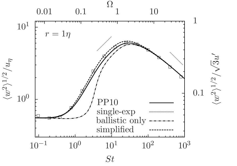
Figure 6.— The 3D rms relative velocity, $\langle w^{2}\rangle^{1/2}$, as a function of the Stokes number, $St$. The data points show the simulation result. The solid line is the prediction of the PP10 model (eq. 30) using a bi-exponential temporal correlation $\Phi_{2}$ and a two-phase separation with $g=1.6$ in the Richardson phase. The dotted line corresponds to the same model but with a single-exponential $\Phi_{2}$. The line is barely visible because it almost coincides with the solid line. The dot-dashed line assumes ballistic separation at all times. The dashed line is the prediction of the simplified model, eqs. (20) and (21), using single-exponential $\Phi_{2}$ and a two-phase separation behavior with $g=1.0$. The top X-axis and the right Y-axis normalize the friction timescale and the relative speed to $T_{\rm L}$ and $\sqrt{3}u^{\prime}$, respectively. The left and right dotted line segments show $St^{1/2}$ and $St^{-1/2}$ scalings.

The solid curve in Fig. (6) is the prediction of the PP10 model, and it is obtained by numerically solving eq. (30). In the computation, we used eq. (8) for $S_{\rm ll}$, eq. (33) for $S_{\rm nn}$, and eq. (23) for $T(\ell)$, respectively. The parameters in these equations were set to $C_{\rm K}=2$, $C_{\rm Kn}=2.5$, $C_{\rm T}=0.4$ and $T_{\rm L}=14.4\tau_{\eta}$. A bi-exponential form, eq. (24), is adopted for the temporal correlation $\Phi_{2}$. We used a two-phase behavior for the particle separation backward in time (§3.4.3), connecting the ballistic and Richardson phases at $\tau_{\rm c}=-\tau_{\rm p}$. We set $d^{2}(\tau)=r^{2}+\langle w^{2}\rangle\tau^{2}$ for $\tau\geq\tau_{\rm c}$, and then switch to the Richardson’s law, $d^{2}(\tau)=d^{2}(\tau_{\rm c})+g\bar{\epsilon}(|\tau|^{3}-|\tau_{\rm c}|^{3})$, for $\tau<\tau_{\rm c}$, where $d^{2}(\tau_{\rm c})=r^{2}+\langle w^{2}\rangle\tau_{\rm c}^{2}$. To fit the simulation data, the Richardson constant, $g$, is set to 1.6. The solid line is in good agreement with the data points, confirming the validity of the physical picture of our model. Adopting a larger $g$ could further improve the fitting quality at intermediate $St$.

In Appendix A, we investigate the backward separation of tracer particles in our simulated flow, and find that $0.5\;\hbox to0.0pt{\lower 2.5pt\hbox{$\sim$}\hss}\raise 1.5pt\hbox{$<$}\;g\;\hbox to0.0pt{\lower 2.5pt\hbox{$\sim$}\hss}\raise 1.5pt\hbox{$<$}\;1.2$. Therefore, the $g$ value used in the solid line in Fig. 6 is significantly larger than that of tracer particles. There exist two possibilities. First, the backward separation of inertial particles in the Richardson phase is indeed faster than tracers. Second, the accuracy of our model for the trajectory structure tensor, $S_{{\rm T}ij}$, may be inadequate. For example, approximating the correlation timescale, $T(\ell)$, in $\Phi_{2}$ by the eddy turnover time at the scale of the particle separation, $R$, is essentially a qualitative assumption. Also there is an order-of-unity uncertainty in the adopted parameter $C_{\rm T}$ for the scaling of $T({\ell})$ in the inertia range (see eq. (23)). If a larger $C_{\rm T}$ were adopted, we could obtain a good fit to the data with a smaller $g$. Finally, in our model for $S_{{\rm T}ij}$, we neglected the correlation between the particle distance, $R$, and the fluctuations in the flow velocity difference, $\Delta u(R)$, seen by the particle pair (see §3.2). This tends to underestimate the relative velocity.

The dotted line in Fig. (6) is the prediction of the same PP 10 model, but with a single-exponential $\Phi_{2}$ (eq. (22)). The dotted line is actually not distinguishable from the solid line, confirming the earlier statement in §3.2.1 that our model prediction for the relative speed is insensitive to the function form of $\Phi_{2}$. This leaves us some freedom for the choice of $\Phi_{2}$, as long as the correlation timescale is accurately esimated. In particular, it provides a justification for approximating $\Phi_{2}$ by the same function form, e.g., a bi-exponential function, for all particles, although realistically the form of $\Phi_{2}$ may have a dependence on the particle inertia.

The dot-dashed curve plots the prediction of the PP10 model assuming that the particle separation is ballistic with $d^{2}(\tau)=r^{2}+\langle w^{2}\rangle\tau^{2}$ at all times. The model is otherwise the same as the solid line. A pure ballistic separation is not realistic, and we show it here just to illustrate whether the Richardson phase provides important contribution to the relative velocity. At $0.5\;\hbox to0.0pt{\lower 2.5pt\hbox{$\sim$}\hss}\raise 1.5pt\hbox{$<$}\;St\;\hbox to0.0pt{\lower 2.5pt\hbox{$\sim$}\hss}\raise 1.5pt\hbox{$<$}\;5$, the dot-dashed line significantly underestimates $\langle w^{2}\rangle$, and, from $St\simeq 5$, it becomes close to both the data points and the solid line using a two-phase separation behavior. A possible explanation for this is that, for $0.5\;\hbox to0.0pt{\lower 2.5pt\hbox{$\sim$}\hss}\raise 1.5pt\hbox{$<$}\;St\;\hbox to0.0pt{\lower 2.5pt\hbox{$\sim$}\hss}\raise 1.5pt\hbox{$<$}\;5$, the relative velocity receives a significant contribution from the Richardson phase, even though this phase occurs at times beyond the particle memory timescale, i.e., at $\tau\;\hbox to0.0pt{\lower 2.5pt\hbox{$\sim$}\hss}\raise 1.5pt\hbox{$<$}\;-\tau_{\rm p}$. In that case, accounting for this phase would be necessary for particles with intermediate $St$. However, the validity of the above interpretation is subject to future tests. There is the possibility that the discrepancy between the dot-dashed line and the data points may be caused by various uncertainties in our model for the trajectory structure tensor, $S_{{\rm T}ij}$ (see above).

The dashed line is the prediction of the simplified model, eqs. (20) and (25), using a single-exponential $\Phi_{2}$. As before, the simplified model with a bi-exponential $\Phi_{2}$ gives almost the same prediction. The same two-phase separation as in the solid line for the original PP10 model is adopted. For the simplified model, the best-fit $g$ is found to be $\simeq 1$, which is close to the $g$ values measured from tracer particles. The simplified model also fits the data better for intermediate $St$, although the assumption made in the model is physically not better than the original PP10 model. The simplified model may be a preferred choice, as its prediction is easier to compute.

We find that the Stokes number, $St_{\rm m}$, at which the rms relative velocity peaks is $\simeq 30$, corresponding to a friction timescale of $\simeq 2T_{\rm L}$ (or $\simeq 1.5T_{\rm eddy}$). The peak value of the 3D rms relative velocity is $\simeq 6.2u_{\eta}$, which is about half the 3D rms velocity ($\sqrt{3}u^{\prime}$) of the flow. We give an explanation for the behavior of the peak relative velocity using the qualitative analysis of our model prediction disucssed in §3.2.4. The analysis was based on the primary distance $R_{\rm p}$, estimated as $R_{\rm p}=\langle w^{2}\rangle^{1/2}\tau_{\rm p}$. $R_{\rm p}$ generally increases with $\tau_{\rm p}$. Around the relative velocity peak, $\tau_{\rm p}\simeq 30\tau_{\eta}$ and $\langle w^{2}\rangle^{1/2}\simeq 6.2u_{\eta}$, and thus $R_{\rm p}\simeq 200\eta$. From eq. (23), the correlation time, $T(\ell)$, at $\ell\simeq 200\eta$ is about $14\tau_{\eta}$, which is close to $T_{\rm L}$. For $St\;\hbox to0.0pt{\lower 2.5pt\hbox{$\sim$}\hss}\raise 1.5pt\hbox{$>$}\;30$, $T(R_{\rm p})$ would be constant and $\simeq T_{\rm L}$. Consequently, the $\Phi_{2}$ term in eq. (30) provides a factor of $T_{\rm L}/\tau_{\rm p}$ for all particles with $St\;\hbox to0.0pt{\lower 2.5pt\hbox{$\sim$}\hss}\raise 1.5pt\hbox{$>$}\;30$ (see §3.2.4). Using the same analysis as in §3.2.4, one can show that this factor causes the relative speed to decrease with $\tau_{\rm p}$, even though the structure functions $S_{\rm ll}(R_{\rm p})$ and $S_{\rm nn}(R_{\rm p})$ are still increasing with $R_{\rm p}$ at $R_{\rm p}\simeq 200\eta$ (see Fig. 3). For particles with $St\;\hbox to0.0pt{\lower 2.5pt\hbox{$\sim$}\hss}\raise 1.5pt\hbox{$<$}\;30$, both the structure functions and $T(R_{\rm p})$ decrease with decreasing $R_{\rm p}$, and thus the relative speed would decrease with decreasing $\tau_{\rm p}$. Therefore a peak forms at $St_{\rm m}\simeq 30$. We find that, for particles with $St\simeq 30$, the amplitude of the flow velocity difference at the primary distance ($R_{\rm p}\simeq 200\eta$) is smaller than $\sqrt{3}u^{\prime}$, and this is responsible for why the maximum relative velocity is significantly lower than the rms flow velocity. The discussion here shows that the relative velocity is the largest for the particles whose primary distance $R_{\rm p}$ corresponds to the size of turbulent eddies with lifetime $\simeq T_{\rm L}$. Clearly, the backward particle separation plays an important role in determining the peak Stokes number, $St_{\rm m}$.

The model of Volk et al. (1980) and its later developments predict that the relative speed reaches the maximum when $\tau_{\rm p}$ is equal to a large eddy time, $t_{\rm L}$ (e.g., Markiewicz, Mizuno & Volk 1991, Cuzzi and Hogan 2003, Ormel & Cuzzi 2007). The definition of $t_{\rm L}$ in these studies is different from the timescales we used, and it is not clear whether, using parameters appropriate for our simulated flow, these models may correctly produce a peak at $St_{\rm m}=30$. Another issue is that, in the Volk et al. model, the peak relative speed is predicted to be equal or close to the rms velocity of the flow. This overestimates the relative speed around the peak by a factor of 2. A physical problem of the Volk et al. model has been discussed in the Introduction (see PP10 for details). The performance of the Volk et al. (1980) model may improve as the Reynolds number of the flow increases, which will be tested by future higher-resolution simulations.

6.1.1 Dependence on the Particle Distance

In Fig. 7, we plot the 3D rms relative velocity at different distances, $r$. The squares, circles and diamonds correspond to $r=1$, $0.5$ and $0.25\eta$, respectively. In this distance range, the relative velocity shows a $r$-dependence at $St\;\hbox to0.0pt{\lower 2.5pt\hbox{$\sim$}\hss}\raise 1.5pt\hbox{$<$}\;6$, while it is independent of $r$ for $St\;\hbox to0.0pt{\lower 2.5pt\hbox{$\sim$}\hss}\raise 1.5pt\hbox{$>$}\;6$ particles. In the context of our physical picture, this is because the friction time, $\tau_{\rm p}$, of $St\;\hbox to0.0pt{\lower 2.5pt\hbox{$\sim$}\hss}\raise 1.5pt\hbox{$>$}\;6$ particles is long enough that the backward particle separation after a duration of $\simeq\tau_{\rm p}$ is insensitive to the “initial” value, $r$. On the other hand, the relative speed of smaller particles relies on the flow velocity difference they saw in the near past, when the particle separation was still dependent on $r$.

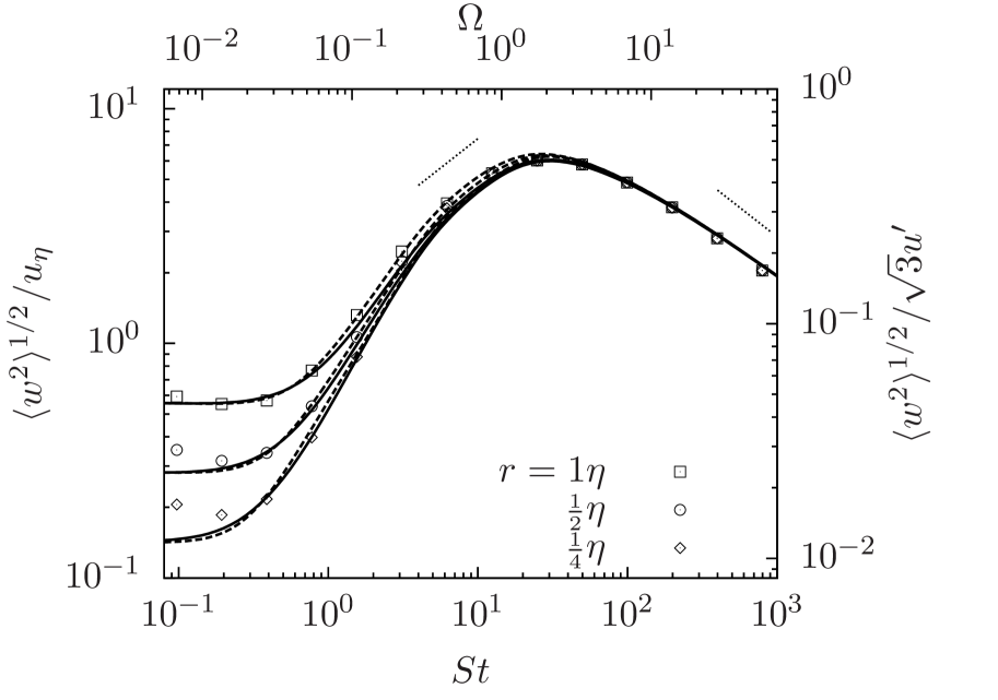
Figure 7.— The 3D rms relative velocity, $\langle w^{2}\rangle^{1/2}$, at at $r=1$ (squares), $0.5$ (circles) and $0.25\eta$ (diamonds). Solid and dashed lines are predictions of the PP10 model with bi-exponential $\Phi_{2}$ and the simplified model with single-exponential $\Phi_{2}$, respectively. A two-phase separation connecting at $\tau=-\tau_{\rm p}$ is adopted in both models. In the PP10 model, the Richardson constant $g$ is set to 1.6, 1.3 and 1.0 for solid lines from top to bottom. The corresponding $g$ values used in the simplified model are 1, 0.7 and 0.5, respectively. The dotted line segments denote $St^{1/2}$ and $St^{-1/2}$ scalings.

The solid and dotted lines are predictions of the PP10 model with bi-exponential correlation function $\Phi_{2}$ and the simplified version with single-exponential $\Phi_{2}$, respectively. The lines for $r=1\eta$ have already been shown in Fig. (6), and the Richardson constant, $g$, was set to 1.6 and 1.0, respectively, in the two models. At smaller $r$, the best-fit value of $g$ becomes smaller. For the PP10 model, we adopted $g=1.3$ and $1.0$ for $r=0.5$ and $0.25\eta$, respectively. The decrease of $g$ with decreasing $r$ is consistent with our result in Appendix A for the tracer particle pair dispersion. The backward separation of tracer pairs was found to be slower for smaller $r$. The $g$ value used in the simplified model also decreases with decreasing $r$. In the dashed lines for $r=1$, $0.5$ and $0.25\eta$, the value of $g$ is set to 1, 0.7 and 0.5, respectively.

The relative speed of the smallest particles ($St\simeq 0.1$) in our simulation appears to be larger than the second smallest ones ($St\simeq 0.2$), especially at smaller $r$. Slight dips are seen at $St\simeq 0.2$ (Fig. 7). This is in contrast to the S-T formula, which predicts the relative speed at a given $r$ is constant at sufficiently small $St$. These dips are not expected from the physical picture of our model either, and their existence is thus questionable. One possibility is that the rise of the relative speed toward $St\simeq 0.1$ is a numerical artifact. This suspicion is based on the consideration that the trajectory integration in our simulation is likely less accurate for smaller particles. The accuracy of the trajectory computation depends on the integration time step relative to the particle friction time. Since the time step is the same for all particles, the accuracy would be lower for smaller particles. This suggests the rise of the relative speed toward $St\simeq 0.1$ may be caused by numerical errors in the trajectory integration. We expect it to disappear as the computation accuracy increases. This will be tested by future simulations with a better temporal resolution for the integration of small particles.

The S-T formula predicts that $\langle w^{2}\rangle^{1/2}$ scales linearly with $r$ in the $St\ll 1$ limit. This linear scaling is not confirmed by our simulation result for the smallest particles. A rough power fit for the rms relative speed as a function of $r$ gives $\langle w^{2}\rangle^{1/2}\propto r^{0.78}$ at $St=0.1-0.2$. This means that, for particles with $St\simeq 0.1-0.2$, the S-T formula is already invalid at $r\;\hbox to0.0pt{\lower 2.5pt\hbox{$\sim$}\hss}\raise 1.5pt\hbox{$<$}\;0.5\eta$. At a given $St$, a critical particle distance is expected, below which the linear scaling does not apply. The physical reason is that, as $r$ decreases, the local flow velocity difference across $r$ becomes smaller, and it is easier for the particle memory of the flow velocity difference in the past to provide a significant contribution, which tends to invalidate the S-T prediction. Equivalently, at a given $r$, the S-T formula is valid only below a critical $St$. In Fig. 7, the lines for $r\;\hbox to0.0pt{\lower 2.5pt\hbox{$\sim$}\hss}\raise 1.5pt\hbox{$<$}\;0.5\eta$ show that, as $St$ decreases to $\simeq 0.2$, the relative speed predicted by our model is not flat yet, suggesting a significant contribution from the particle memory. At sufficiently small $St$, the rms relative speed at a distance $r\;\hbox to0.0pt{\lower 2.5pt\hbox{$\sim$}\hss}\raise 1.5pt\hbox{$<$}\;0.5\eta$ is expected to finally become constant. To verify this, a simulation of higher accuracy for small particles is needed to fix the problem of the artificial rise in the relative velocity toward $St\simeq 0.1$. As mentioned earlier, the rise is expected to disappear as the computation accuracy for the smallest particles increases.

Our model does not directly consider the sling effect (Falkovich et al. 2002, Falkovich and Pumir 2007) or the related caustic formation (Wilkinson & Mehlig 2005; Wilkinson et al. 2006; Gustavsson & Mehlig 2011). The effect of slings is usually explored for small particles with $St\;\hbox to0.0pt{\lower 2.5pt\hbox{$\sim$}\hss}\raise 1.5pt\hbox{$<$}\;1$. As mentioned in the Introduction, it corresponds to crossing of particle trajectories that occurs at fluid streamlines with high curvature or local flow regions with large velocity gradient. In our physical picture, the effect of slings or caustics could be viewed as a contribution to the backward particle separation. In the sling events, the particle pairs come together from a farther distance than the average. Based on the model of Wilkinson et al. (2006) and Gustavsson & Mehlig (2011), the frequency of slings or caustic formation increases with $St$. The effect also becomes more important as $r$ decreases, and would finally dominate over the S-T contribution at a sufficiently small $r$. Falkovich and Pumir (2007) showed that the sling effect is already significant at $St\simeq 0.2$. In Fig. 7, we see that our model prediction underestimates the relative velocity of $St=0.2$ particles at $r\;\hbox to0.0pt{\lower 2.5pt\hbox{$\sim$}\hss}\raise 1.5pt\hbox{$<$}\;0.5\eta$. A likely reason is that the sling effect is not sufficiently reflected by the assumed backward separation behavior. In principle, the effect can be better incorporated into our model by directly and accurately evaluating the frequency of such events and their contribution to the backward separation. We will discuss the effect of slings or caustics on the particle collision rate in details in §7. For $St\;\hbox to0.0pt{\lower 2.5pt\hbox{$\sim$}\hss}\raise 1.5pt\hbox{$<$}\;1$ particles, the sling events are rare. At $St\;\hbox to0.0pt{\lower 2.5pt\hbox{$\sim$}\hss}\raise 1.5pt\hbox{$>$}\;3$, these events become very frequent, and essentially all particle pairs at $r\;\hbox to0.0pt{\lower 2.5pt\hbox{$\sim$}\hss}\raise 1.5pt\hbox{$<$}\;\eta$ should be counted as sling or caustic pairs (§7.2). In our physical picture, this corresponds to the fact that the backward separation of $St\;\hbox to0.0pt{\lower 2.5pt\hbox{$\sim$}\hss}\raise 1.5pt\hbox{$>$}\;3$ particle pairs at a friction timescale ago is significantly larger the initial distance, $r$.

Concerning the $r$-dependence of $\langle w^{2}\rangle^{1/2}$ for $St\;\hbox to0.0pt{\lower 2.5pt\hbox{$\sim$}\hss}\raise 1.5pt\hbox{$<$}\;6.2$ particles seen in Fig. 7, a fundamental question is whether the dependence disappears as $r$ further decreases below $\eta/4$, or, equivalently, whether $\langle w^{2}\rangle^{1/2}$ approaches a finite constant as $r\to 0$. Based on the prediction of Gustavsson & Mehlig (2011), it is possible that, for particles that exhibit significant clustering (see §7.1), the overall rms relative velocity may approach 0 as $r\to 0$. In the case, $\langle w^{2}\rangle^{1/2}$ for $St\;\hbox to0.0pt{\lower 2.5pt\hbox{$\sim$}\hss}\raise 1.5pt\hbox{$<$}\;6.2$ particles would not converge with decreasing $r$, and thus in principle could not be resolved. Intuitively, the rms relative speed, $\langle w^{2}\rangle^{1/2}$, of intermediate particles with $1\;\hbox to0.0pt{\lower 2.5pt\hbox{$\sim$}\hss}\raise 1.5pt\hbox{$<$}\;St\;\hbox to0.0pt{\lower 2.5pt\hbox{$\sim$}\hss}\raise 1.5pt\hbox{$<$}\;6.2$ may converge at sufficiently small $r$, while, for $St\ll 1$ particles, $\langle w^{2}\rangle^{1/2}$ may decrease to zero as $r\to 0$. The convergence of $\langle w^{2}\rangle^{1/2}$ for $St\;\hbox to0.0pt{\lower 2.5pt\hbox{$\sim$}\hss}\raise 1.5pt\hbox{$<$}\;6.2$ particles needs to checked with larger simulations that allow accurate measurements at $r\ll\eta/4$.

6.1.2 The Radial and Tangential Relative Speeds

Fig. 8 shows the rms relative speeds in the radial (circles) and tangential (diamonds) directions for particle pairs at $r=1$, $0.5$ and $0.25\eta$. At $St\;\hbox to0.0pt{\lower 2.5pt\hbox{$\sim$}\hss}\raise 1.5pt\hbox{$<$}\;1$, the tangential rms speed, $\langle w_{\rm t}^{2}\rangle^{1/2}$, is slightly larger (by $\simeq 10\%$) than the radial rms, $\langle w_{\rm r}^{2}\rangle^{1/2}$. This difference is considerably smaller than the prediction of the S-T formula, eq. (11), which indicates that for $St\ll 1$ particles the tangential rms relative speed should be larger than the radial rms by a factor of $\sqrt{2}$. Our data implies that this prediction is not valid at least for particles with $St\;\hbox to0.0pt{\lower 2.5pt\hbox{$\sim$}\hss}\raise 1.5pt\hbox{$>$}\;0.1$. It remains to be checked whether the factor of $\sqrt{2}$ difference between $\langle w_{\rm r}^{2}\rangle^{1/2}$ and $\langle w_{\rm t}^{2}\rangle^{1/2}$ would be recovered at smaller Stokes numbers. In Fig. 8, we see that $\langle w_{\rm r}^{2}\rangle^{1/2}$ and $\langle w_{\rm t}^{2}\rangle^{1/2}$ become exactly equal at $St\;\hbox to0.0pt{\lower 2.5pt\hbox{$\sim$}\hss}\raise 1.5pt\hbox{$>$}\;1$.

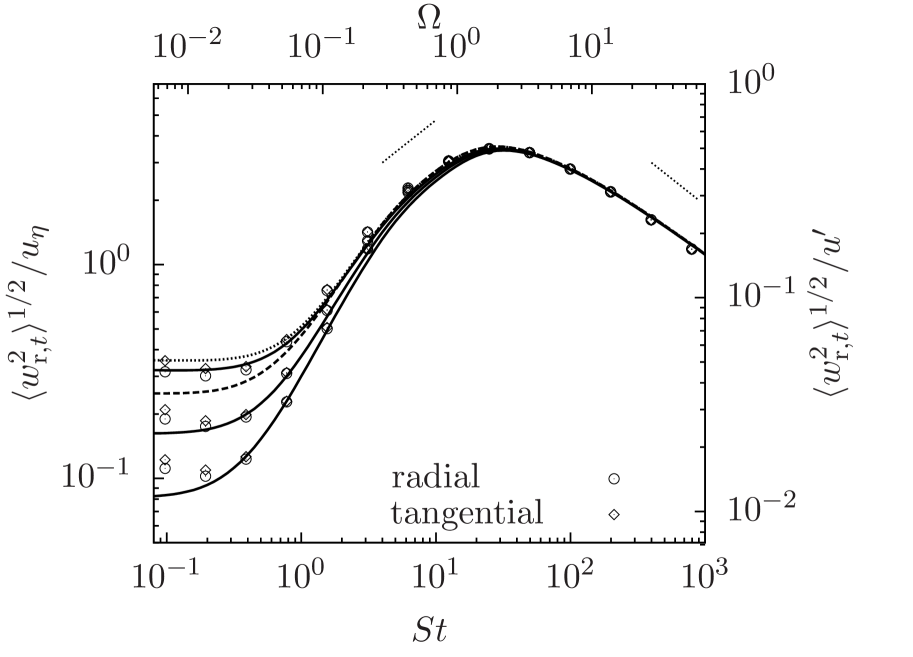
Figure 8.— The rms relative speeds in the radial ($\langle w_{\rm r}^{2}\rangle^{1/2}$; circles) and tangential ($\langle w_{\rm t}^{2}\rangle^{1/2}$; diamonds) directions. From top to bottom, data points show simulation results at $r=1$, $0.5$, and $0.25\eta$, respectively. Lines are predictions of the PP10 model. The solid lines adopt eq. (27) for the angular average of $S_{{\rm T}ij}$, which predicts that $\langle w_{\rm r}^{2}\rangle=\langle w_{\rm t}^{2}\rangle=\frac{1}{3}\langle w^{2}\rangle$. The particle separation behavior assumed here is exactly the same as in the solid lines in Fig. 7 for the 3D rms. The Richardson constant, $g$, is set to 1.6, 1.3 and 1.0 for $r=1$, $0.5$, and $0.25\eta$, respectively. The dashed and dotted lines for $r=1\eta$ are solutions of eq. (31) for the radial and tangential relative speeds, respectively. The two lines reproduce the S-T prediction for $\langle w_{\rm r}^{2}\rangle^{1/2}$ and $\langle w_{\rm t}^{2}\rangle^{1/2}$ at $St\ll 1$.

The solid lines in Fig. 8 correspond to the prediction of the PP10 model using eq. (27) for the angular average, $\langle S_{{\rm T}ij}\rangle_{\rm ang}$, of the trajectory structure tensor. The equation assumes that the direction of the particle separation ${\boldsymbol{R}}$ at any time is completely random, and predicts that $\langle w_{\rm r}^{2}\rangle=\langle w_{\rm t}^{2}\rangle=\frac{1}{3}\langle w^{2}\rangle$ for all particles (§3.2.2). This prediction is in good agreement with our simulation data. The equality of the radial and tangential rms speeds for $St\;\hbox to0.0pt{\lower 2.5pt\hbox{$\sim$}\hss}\raise 1.5pt\hbox{$>$}\;1$ is expected, because the separation ${\boldsymbol{R}}$ of these particles at a friction timescale ago is significantly larger than the initial distance, $r$, and its direction is likely random with respect to ${\boldsymbol{r}}$. On the other hand, the near equality of $\langle w_{\rm r}^{2}\rangle^{1/2}$ and $\langle w_{\rm t}^{2}\rangle^{1/2}$ at $St\sim 0.1-0.2$ is somewhat surprising. For $r=1\eta$, the backward separation of these particles does not contribute to make the 3D rms, $\langle w^{2}\rangle^{1/2}$, of the relative velocity significantly larger than the S-T prediction. This suggests that the near equality of $\langle w_{\rm r}^{2}\rangle^{1/2}$ and $\langle w_{\rm t}^{2}\rangle^{1/2}$ is due to a conversion of the relative velocity from the tangential to the radial direction. The conversion is probably caused by the deviation of the particle trajectories from the fluid elements. Even though the deviation does not considerably change the 3D amplitude $\langle w^{2}\rangle^{1/2}$ at $r\simeq 1\eta$, it could efficiently alter the direction of ${\boldsymbol{w}}$ with respect to ${\boldsymbol{r}}$. The trajectory deviation is stochastic, and thus tends to randomize the direction of ${\boldsymbol{w}}$ and equalize its radial and tangential components. This reduces the tangential-to-radial ratio. The randomization effect is expected to be more efficient in the slings events, where the particles are shot out of the flow streamlines, and encounter the trajectories of other particles. At smaller $r$, the contribution from the backward separation to the 3D rms of the relative velocity is larger, and the random direction of the particle separation in the past also tends to equalize the radial and tangential components. In the $r\to 0$ limit, we would expect that $\langle w_{\rm r}^{2}\rangle^{1/2}$ and $\langle w_{\rm t}^{2}\rangle^{1/2}$ are exactly equal at all $St$.

When computing the solid lines, we used a bi-exponential form for $\Phi_{2}$, and the separation behavior adopted here is exactly the same as for the solid lines in Fig. 7 for the 3D rms. The solid lines shown here correspond to those in Fig. 7 divided by $\sqrt{3}$. The Richardson constant is set to 1.6, 1.3 and 1.0 in the three lines for $r=1,0.5$, and $0.25\eta$, respectively.

The dashed and dotted lines for $r=1\eta$ are the solutions of eq. (31) for the radial and tangential rms relative speeds, respectively. Eq. (31) was derived from eq. (26) for $\langle S_{{\rm T}ij}\rangle_{\rm ang}$, which assumes that the direction of the separation change $\Delta{\boldsymbol{R}}$ (rather than ${\boldsymbol{R}}$ itself) is random. When solving eq. (31), we used the same two-phase separation behavior (with $g=1.6$) as in the corresponding solid line. At small $St$, the dashed and solid lines reproduce the S-T prediction that $\langle w_{\rm t}^{2}\rangle=2\langle w_{\rm r}^{2}\rangle$. The discrepancy between the simulation data and the S-T formula implies that, for particles with $0.1\;\hbox to0.0pt{\lower 2.5pt\hbox{$\sim$}\hss}\raise 1.5pt\hbox{$<$}\;St\;\hbox to0.0pt{\lower 2.5pt\hbox{$\sim$}\hss}\raise 1.5pt\hbox{$<$}\;1$, the direction of ${\boldsymbol{R}}$ is more random than assumed in eq. (26).

The dependence of the radial and tangential rms relative speeds on $r$ is similar to that of the 3D rms (see Fig. 7). In an attempt to roughly fit them as power-law functions of $r$, we find that $\langle w_{\rm r}^{2}\rangle^{1/2}$and $\langle w_{\rm t}^{2}\rangle^{1/2}$ scale with $r$ as $\propto r^{0.78}$ at $St=0.1-0.2$. Similar to the 3D rms, the slight dips at $St\simeq 0.2$ for both $\langle w_{\rm r}^{2}\rangle^{1/2}$and $\langle w_{\rm t}^{2}\rangle^{1/2}$ may be due to a numerical artifact.

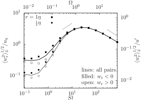
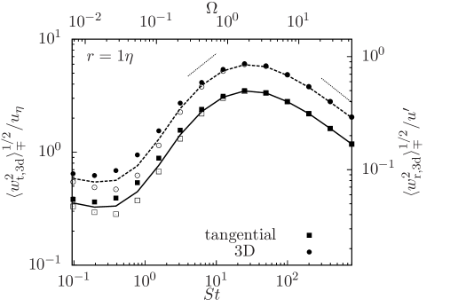
Figure 9.— The rms relative speeds for approaching ($w_{\rm r}<0$; filled symbols) or separating ($w_{\rm r}>0$; open symbols) particle pairs. Lines correspond to the overall rms relative speeds counting all pairs. Left panel: The radial rms speed $\langle w_{\rm r}^{2}\rangle_{\mp}^{1/2}$) in the minus and plus groups with $r=1\eta$ (squares) and $0.25\eta$ (circles). Right panels: the tangential (squares) and 3D (circles) rms relative speeds for particle pairs at $r=1\eta$. The dotted line segments denote $St^{1/2}$ and $St^{-1/2}$ scalings.

The simulations of Wang et al. (2000) found that the tangential-to-radial variance ratio, $\langle w_{\rm t}^{2}\rangle/\langle w_{\rm r}^{2}\rangle$, is $\simeq 1.5-1.6$ at $St\simeq 0.1-0.2$. This is closer to the S-T prediction and larger than the corresponding value ($1.2-1.3$) in our simulation. This is probably because our flow has a much larger Reynolds number. Although Wang et al. (2000) claimed that the ratio is independent of $Re_{\lambda}$ based on several simulations with $Re_{\lambda}\;\hbox to0.0pt{\lower 2.5pt\hbox{$\sim$}\hss}\raise 1.5pt\hbox{$<$}\;75$, it is not clear if this is also true at $Re_{\lambda}\gg 75$. As speculated above, it is the deviation of the particle trajectories from the flow elements that tends to equalize the radial and tangential relative speeds of small particles. Clearly, the trajectory deviation would be larger in flow regions with larger velocity gradients, where the flow experiences a faster velocity change. The probability of finding large flow velocity gradients hence large trajectory deviations increases with $Re_{\lambda}$. Therefore, the tangential-to-radial ratio is likely smaller at higher $Re_{\lambda}$. For $St\;\hbox to0.0pt{\lower 2.5pt\hbox{$\sim$}\hss}\raise 1.5pt\hbox{$<$}\;1$ particles, the sling events occur in regions with extreme flow velocity gradients, and the frequency of slings would increase with $Re_{\lambda}$ (Falkovich and Pumir 2007). This also tends to reduce the tangential-to-radial ratio. However, we cannot rule out the possibility that the trajectory integration of the smallest particles in our simulation is not sufficiently accurate to allow an accurate measurement of $\langle w_{\rm t}^{2}\rangle/\langle w_{\rm r}^{2}\rangle$ at small $St$.

6.1.3 Approaching and Separating Particle Pairs

So far, our analysis for the particle relative velocity included all particle pairs at given distances. However, not all pairs at a small distance lead to collisions. Particles with a negative radial relative velocity, $w_{\rm r}<0$, approach each other and may collide, while particle pairs with $w_{\rm r}>0$ move away from each other. Since the final goal of our study is to examine the particle collisions, it is appropriate to split particle pairs at a given distance into two groups with $w_{\rm r}<0$ and $w_{\rm r}\geq 0$, respectively. We refer to them as the minus and plus groups. Although only the first group is relevant for particle collisions, it is theoretically interesting to compare the two groups.

For the radial component, $w_{\rm r}$, of the relative velocity, we denote the variances in the minus and plus groups as $\langle w_{\rm r}^{2}\rangle_{-}$ and $\langle w_{\rm r}^{2}\rangle_{+}$, respectively. In terms of the PDF, $P(w_{\rm r},St)$, of $w_{\rm r}$, the variances are written as $\langle w_{\rm r}^{2}\rangle_{-}=\int_{-\infty}^{0}w_{\rm r}^{2}P(w_{\rm r},St)dw_{\rm r}/\int_{-\infty}^{0}P(w_{\rm r},St)dw_{\rm r}$ and $\langle w_{\rm r}^{2}\rangle_{+}=\int_{0}^{\infty}w_{\rm r}^{2}P(w_{\rm r},St)dw_{\rm r}/\int_{0}^{\infty}P(w_{\rm r},St)dw_{\rm r}$. We denote the PDFs of the tangential component in the minus and plus groups as conditional PDFs, $P(w_{\rm t}|w_{\rm r}<0,St)$ and $P(w_{\rm t}|w_{\rm r}>0,St)$. The tangential variances in the two groups are then given by $\langle w_{\rm t}^{2}\rangle_{\mp}=\int_{-\infty}^{\infty}w_{\rm t}^{2}P(w_{\rm t}|w_{\rm r}\lessgtr 0,St)dw_{\rm t}$. Similarly, for the 3D amplitude, $|{\boldsymbol{w}}|$, the minus and plus variances are expressed as $\langle w^{2}\rangle_{\mp}=\int_{-\infty}^{\infty}w^{2}P(|{\boldsymbol{w}}||w_{\rm r}\lessgtr 0,St)d|{\boldsymbol{w}}|$, where $P(|{\boldsymbol{w}}||w_{\rm r}\lessgtr 0,St)$ are the PDFs of $|{\boldsymbol{w}}|$ for approaching and separating pairs. The PDFs, $P(w_{\rm r},St)$, $P(w_{\rm t}|w_{\rm r}\lessgtr 0,St)$, and $P(|{\boldsymbol{w}}||w_{\rm r}\lessgtr 0,St)$, will be studied in §6.2.

The data points in the left panel of Fig. (9) show the radial rms relative speeds of particle pairs at $r=1\eta$ (squares) and $0.25\eta$ (circles). The right panel plots the tangential (squares) and 3D (circles) rms speeds at $1\eta$. In both panels, the filled and open symbols correspond to particle pairs in the minus and plus groups, respectively, and the lines plot the overall rms relative velocities counting all particle pairs. If the velocity of $St\ll 1$ particles closely follow the flow velocity, we expect that $\langle w_{\rm r}^{2}\rangle_{\mp}$ are determined by the variances of the longitudinal flow velocity increments, $\langle\Delta u_{\rm r}^{2}\rangle_{\mp}$, for negative and positive $\Delta u_{\rm r}$, respectively. The definition of $\langle\Delta u_{\rm r}^{2}\rangle_{\mp}$ is given in Appendix B, and they correspond to the fluctuation amplitudes in the left and right wings of the PDF of $\Delta u_{\rm r}$. In Appendix B, we find the ratio $\langle\Delta u_{\rm r}^{2}\rangle_{-}/\langle\Delta u_{\rm r}^{2}\rangle_{+}$ is 1.47 at the size, $\Delta x$, of the computation cell. This suggests that, in the $St\to 0$ limit, $\langle w_{\rm r}^{2}\rangle_{-}^{1/2}$ would be larger than $\langle w_{\rm r}^{2}\rangle_{+}^{1/2}$ by $\simeq 20\%$. The simulation result confirms this expectation. At $St\simeq 0.1$, $\langle w_{\rm r}^{2}\rangle_{-}^{1/2}$ is larger than $\langle w_{\rm r}^{2}\rangle_{+}^{1/2}$ by $\simeq 25\%$ for both $r=1$ and $0.25\eta$ (see the left panel of Fig. 9). Using a similar analysis to the tangential component gives $\langle w_{\rm t}^{2}\rangle_{\mp}^{1/2}\simeq\langle\Delta u_{\rm t}^{2}\rangle_{\mp}^{1/2}$ for $St\ll 1$, where $\langle\Delta u_{\rm t}^{2}\rangle_{\mp}$ are variances of the transverse flow velocity increment, $\Delta u_{\rm t}$, conditioned on the sign of the longitudinal increment $\Delta u_{\rm r}$ (see Appendix B). The ratio $\langle w_{\rm t}^{2}\rangle_{-}^{1/2}/\langle w_{\rm t}^{2}\rangle_{+}^{1/2}$ is found to be 1.16 at $St=0.1-0.2$, consistent with the ratio of $\langle\Delta u_{\rm t}^{2}\rangle_{-}$ to $\langle\Delta u_{\rm t}^{2}\rangle_{+}$ at the grid cell size, $\Delta x$ (see Appendix B). For the the 3D amplitude ($\langle w^{2}\rangle_{\mp}^{1/2}$), the rms ratio between the minus and plus groups is 1.18 at $St\ll 1$.

As $St$ increases, the relative speed for the plus group first decreases slightly and reaches a minimum at $St\simeq 0.4$ in all cases with $r=1\eta$. This can be explained by considering the effects of the particle memory and the particle separation backward in time. Particle pairs in the plus group with $w_{\rm r}>0$ are coming from smaller distances, meaning that the separation of the particles was smaller in the near past. As $St$ increases from 0.1 to 0.4, the contribution from the particle memory of the flow velocity difference becomes more important, and this contribution tends to reduce the relative speed since the particle distance was smaller in the immediate past. However, if we look back further into the past (i.e., at larger $|\tau|$), the two particles may pass each other, and their distance would make a transition from decreasing to increasing. This explains the increase of $\langle w_{\rm r}^{2}\rangle_{+}$, $\langle w_{\rm t}^{2}\rangle_{+}$, and $\langle w^{2}\rangle_{+}$ at $St\;\hbox to0.0pt{\lower 2.5pt\hbox{$\sim$}\hss}\raise 1.5pt\hbox{$>$}\;0.4$. The minimum of $\langle w_{\rm r}^{2}\rangle_{+}$ for $r=0.25\eta$ appears at $St=0.2$ instead of $St=0.4$, because, for smaller $r$, it takes a shorter time for the particle distance in the past to change from decreasing to increasing.

For approaching particles in the minus group, the particle distance would increase monotonically toward the past. Therefore, the relative speed for this group is expected to increase monotonically as $\tau_{\rm p}$ increases from 0 to $\simeq T_{\rm L}$. This is confirmed by the filled data points in Fig. 9, except the slight dips at $St\simeq 0.2$. These dips are not expected, and again may be caused by insufficient numerical accuracy in the trajectory integration of the smallest particles (§6.1.1). Fig. 9 shows that approaching particles tend to have a larger relative speed than separating ones. The difference between the two groups first increases with $St$ and then decreases at $St\geq 1$. At $St\;\hbox to0.0pt{\lower 2.5pt\hbox{$\sim$}\hss}\raise 1.5pt\hbox{$>$}\;6.2$, the rms relative speeds in the two groups are close and coincide with the overall rms. The reason is that, for these larger particles, the separation of the particle pairs in the two groups at a friction timescale ago becomes insensitive to the “initial” condition around $\tau=0$.

The asymmetry in the relative velocity of $St\;\hbox to0.0pt{\lower 2.5pt\hbox{$\sim$}\hss}\raise 1.5pt\hbox{$<$}\;6.2$ particles is related to the spatial clustering of these particles. The fact that approaching pairs move faster than separating ones may imply that particles tend to cluster at small distances to a reference particle (see also §7.1). An interesting question is whether the asymmetry found at $\eta/4\;\hbox to0.0pt{\lower 2.5pt\hbox{$\sim$}\hss}\raise 1.5pt\hbox{$<$}\;r\;\hbox to0.0pt{\lower 2.5pt\hbox{$\sim$}\hss}\raise 1.5pt\hbox{$<$}\;\eta$ would exist also in the $r\to 0$ limit. We expect the asymmetry to decrease with decreasing $r$ because the difference caused by the different separation behaviors in the near past for approaching and separating pairs would be smaller at smaller $r$. However, it is not clear whether it completely vanishes as $r\to 0$. For example, the asymmetry in the flow velocity difference, $\Delta{\boldsymbol{u}}$, persists at any tiny but finite $r$, and it may leave an imprint on the relative velocity of small particles (say, with $St\;\hbox to0.0pt{\lower 2.5pt\hbox{$\sim$}\hss}\raise 1.5pt\hbox{$<$}\;1$). The actual behavior of the asymmetry as $r\to 0$ will be checked by future simulations that allow to resolve smaller $r$. The prediction of the PP10 model was made only for the overall rms, and it could be modified to give separate predictions for approaching and separating pairs if the different separation behaviors of the two groups are properly specified. We also find that $\langle w_{\rm r}^{2}\rangle_{-}^{1/2}$ and $\langle w_{\rm t}^{2}\rangle_{-}^{1/2}$ almost coincide for all $St$, suggesting that each relative velocity component would provide equal amount of collision energy. On average, the radial component contributes 1/3 collision energy, while the rest 2/3 is from the two tangential components.

6.2. The PDF of the Particle Relative Velocity

An accurate estimate of the PDF of the particle collision velocity is important for modeling the growth and evolution of dust particles in protoplanetary disks. As mentioned in the Introduction, the outcome of particle collisions depends on the collision velocity, and due to the random nature of the turbulent-induced collision velocity, collisions of particles with exactly the same properties may have different outcomes, and thus using a single value, e.g., the rms, for the collision speed of particles of a given size is insufficient. The probability distribution of the collision velocity is needed to calculate the fractions of collisions resulting in sticking, bouncing or fragmentation.

In this section, we explore the probability distribution of the particle relative velocity. We will primarily show the PDFs at $r=\eta$, where the statistical measurements are most sufficient and accurate. The measured PDFs for $St\;\hbox to0.0pt{\lower 2.5pt\hbox{$\sim$}\hss}\raise 1.5pt\hbox{$>$}\;10$ particles already converge at $r\simeq\eta$. On the other hand, for smaller particles the PDFs have an $r$-dependence at $r\;\hbox to0.0pt{\lower 2.5pt\hbox{$\sim$}\hss}\raise 1.5pt\hbox{$>$}\;\eta/4$, and an appropriate extrapolation to $r\to 0$ using larger simulations will be needed for the application to dust particle collisions.

The physical picture of PP10 shows that the relative velocity of inertial particles depends on the flow velocity difference the particle pairs saw within a memory timescale or so. This suggests that the statistics of the velocity difference in the carrier flow is crucial for the understanding of the relative velocity PDF of inertial particles. Therefore, we analyzed the PDFs, $P_{\rm u}(\Delta u_{\rm r},\ell)$ and $P_{\rm u}(\Delta u_{\rm t},\ell)$, of the longitudinal and transverse velocity increments, $\Delta u_{\rm r}$ and $\Delta u_{\rm t}$, as functions of the length scale, $\ell$, in our simulated flow. The results are discussed in details in Appendix B. The flow velocity PDFs are used in the physical explanation for the PDF of the particle relative velocity as a function of particle inertia in §6.2.2.

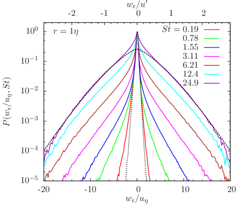
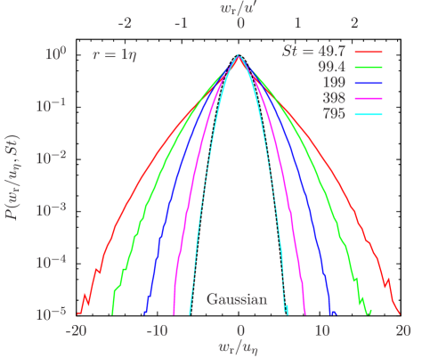
Figure 10.— The PDF of the radial component ($w_{\rm r}$) of the relative velocity at $r=1\eta$ as a function of $St$. The relative speed is normalized by the Kolmogorov velocity, $u_{\eta}$, and the rms flow velocity, $u^{\prime}$, on bottom and top axises, respectively. Each PDF is normalized to its peak value at $w_{\rm r}=0$. The left panel shows the PDFs for particles with $St\leq 24.9$, while the right panel shows results for $St\geq 49.7$ particles. The dotted line in the left panel is the PDF of the radial relative speed of tracer particles ($St=0$). The dashed line in this panel is the stretched exponential function with $\alpha=4/3$, which provides a good fit for the PDF tails of $St=24.9$ particles. In the right panel, the dashed line corresponds to the Gaussian fit to the largest particles in our simulation. One can use $\Omega=St/14.4$ and $\Omega_{\rm eddy}=St/19.2$ to convert the normalization of the particle friction time.

6.2.1 The PDFs of the radial and tangential components

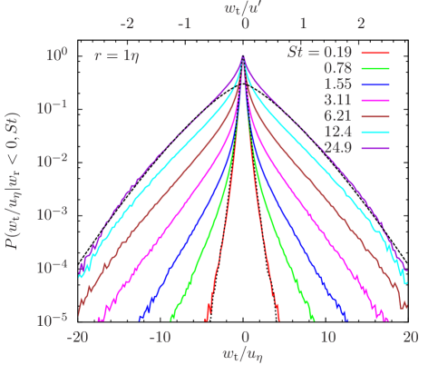
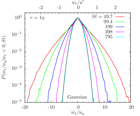
Figure 11.— The PDFs of the tangential relative velocity, $w_{\rm t}$, conditioned on $w_{\rm r}<0$. The PDFs are measured from approaching particle pairs. The normalizations are the same as in Fig. 10. The left and right panels show results for particles with $St\leq 24.9$ and $St\geq 49.7$, respectively. The dotted line in the left panel is the PDF of the tangential relative velocity of tracer particles ($St=0$) conditioned on $w_{\rm r}<0$. The dashed line in this panel is a stretched exponential function with $\alpha=4/3$. The dashed line in the right panel corresponds to the Gaussian fit for $St=795$ particles.

In Fig. 10, we show the PDF, $P(w_{\rm r},St)$, of the radial component of the relative velocity as a function of the Stokes number. All the PDFs are measured at a particle distance of $1\eta$. The relative speed is normalized to the Kolmogorov velocity, $u_{\eta}$, and the 1D flow rms velocity, $u^{\prime}$, on the bottom and top X-axises, respectively. Each PDF is normalized to its value at the central peak. In the left panel, the thin dashed line corresponds to the PDF of tracer particles ($St=0$) at $1\eta$. The shape of this line is found to be identical to the PDF, $P_{\rm u}(\Delta u_{\rm r},\ell)$, of the longitudinal flow velocity increment, $\Delta u_{\rm r}$, at the computational cell size ($\ell=1.7\eta$; see the top line in the left panel of Fig. 21 in Appendix B). This is expected as tracer particles exactly follow the flow velocity, and the shape of $P_{\rm u}(\Delta u_{\rm r},\ell)$ is independent of $\ell$ in the dissipation range (Appendix B). The solid color lines of increasing width show the PDFs of larger particles. This corresponds to the increase of the rms relative speed with $St$ for $St\;\hbox to0.0pt{\lower 2.5pt\hbox{$\sim$}\hss}\raise 1.5pt\hbox{$<$}\;24.9$ (see Figs. 8 and 9). For $St\leq 1.55$, the PDF of $w_{\rm r}$ has a negative skewness, which is inherited from the flow velocity PDF $P_{\rm u}(\Delta u_{\rm r},\ell)$. The PDF becomes symmetric at $St\;\hbox to0.0pt{\lower 2.5pt\hbox{$\sim$}\hss}\raise 1.5pt\hbox{$>$}\;3.21$. It is interesting to note that, as $St$ increases, the tails of the PDFs become broader, while the innermost part remains unaffected and the same as the PDF of the tracer particles. As to be shown in §6.2.2, the amplification of the PDF tails correspond to the effect of slings or caustic formation. Due to the tail amplification, the overall PDF shape becomes fatter as $St$ increases to $\simeq 1.55$. With increasing $St$, the amplification effect proceeds towards the inner parts of the PDF, leading to a sharp cusp-like shape at the center, especially for $St\;\hbox to0.0pt{\lower 2.5pt\hbox{$\sim$}\hss}\raise 1.5pt\hbox{$>$}\;3.11$. For particles with $St\;\hbox to0.0pt{\lower 2.5pt\hbox{$\sim$}\hss}\raise 1.5pt\hbox{$>$}\;3.11$, the slope of the outer parts of the PDF tends to steepen when extending to higher tails, i.e., the PDF shape becomes thinner at larger $|w_{\rm r}|$. This thinning trend toward the high tails causes a decrease in the overall fatness of the PDF for $St$ above $3.11$.

In the right panel, the PDF becomes narrower as $St$ increases above $49.7$, corresponding to the decrease of the rms relative velocity with $St$ in the large particle limit (Figs. 8 and 9). For $St\geq 49.7$ ($\Omega\geq 3.4$), the friction timescale is larger than the correlation timescale ($T_{\rm L}$) of the flow velocity at largest scales, meaning that the memory time of the flow velocity is shorter than the memory of the particles. This induces a factor of $T_{\rm L}/\tau_{\rm p}$ in the relative velocity variance (§3.2.4), causing a decrease of the PDF width at larger $St$. The dotted line in the right panel is the Gaussian fit to the PDF of the largest particles ($St=795$; or $\Omega=54$) in our simulation. For these particles, $\tau_{\rm p}$ is 54 times larger than $T_{\rm L}$, suggesting that the assumption of a Gaussian relative velocity PDF applies only in the extreme limit $\tau_{\rm p}\gg T_{\rm L}$.

Fig. 11 shows the PDF, $P(w_{\rm t}|w_{\rm r}<0,\tau_{\rm p})$, of a tangential component of the relative velocity conditioned on $w_{\rm r}<0$. The measurement of $P(w_{\rm t}|w_{\rm r}<0,\tau_{\rm p})$ only counts particle pairs approaching each other. The figure is plot in the same way as Fig. 10 for the radial component. Again, the thin dashed line in the left panel is for tracer particles ($St=0$). It corresponds to the PDF of the transverse difference, $\Delta u_{\rm t}$, of the flow velocity conditioned on $\Delta u_{\rm r}<0$. The shape of $P(w_{\rm t}|w_{\rm r}<0,0)$ for tracer particles at $r=1\eta$ is close to the dashed line in the right panel of Fig. 21 for $P_{\rm u}(\widetilde{\Delta u_{\rm t}}|\Delta u_{\rm r}<0,\ell)$ at $\ell=1.7\eta$ (Appendix B). The qualitative behavior of $P(w_{\rm t}|w_{\rm r}<0,St)$ as a functions of $St$ is similar to that of $P(w_{\rm r},St)$.

For $St=0.19$ particles, the radial PDF tails are significantly amplified with respect to tracers (Fig. 10), while the conditional PDF of the tangential component almost coincides with the tracer PDF (Fig. 11). From the physical picture for the PDF behavior given in §6.2.2, the effects of the particle memory and the backward separation tend to amplify the PDF tails of $St=0.19$ particles. For the tangential PDF, this amplification effect is counteracted by the conversion of the relative velocity from the tangential to the radial direction, which reduces the PDF width of the tangential component. As discussed in §6.1.2, the conversion is caused by the deviation of inertial particle trajectories from the flow elements and the particle memory of the flow velocity in the past, which randomize the direction of $\boldsymbol{w}$ relative to the particle separation, ${\boldsymbol{r}}$. The conversion is expected to be more efficient at the PDF tails (corresponding to the sling events). It appears that the two opposite effects cancel out for the tangential PDF of $St\simeq 0.19$ particles, as it almost coincides with the dotted line for tracers. On the other hand, both effects broaden the PDF of the radial component, leading to significantly amplified tails with respect to tracers.

Unlike $P(w_{\rm r},St)$, which has a negative skewness for $St\leq 1.55$ particles, $P(w_{\rm t}|w_{\rm r}<0,St)$ is symmetric at all $St$. As mentioned earlier, the symmetry of the tangential PDF is expected from the statistical isotropy. We find that the left wing of the radial PDF $P(w_{\rm r},St)$ almost coincides with that of $P(w_{\rm t}|w_{\rm r}<0,St)$ at all $St$. This is apparently due to the randomization of the relative velocity direction discussed above. On the other hand, the right wing of $P(w_{\rm r},St)$ is narrower than that of $P(w_{\rm r}|w_{\rm r}<0,St)$, until it becomes symmetric at $St\;\hbox to0.0pt{\lower 2.5pt\hbox{$\sim$}\hss}\raise 1.5pt\hbox{$>$}\;3.11$. To study particle collisions, we are mainly interested in the PDFs for approaching pairs, i.e., the left wing of $P(w_{\rm r},St)$ and the entire tangential PDF, $P(w_{\rm t}|w_{\rm r}<0,St)$, conditioned on $w_{\rm r}<0$.

We give a more quantitative description for the shape of $P(w_{\rm t}|w_{\rm r}<0,St)$. The description also applies to the left wing of $P(w_{\rm r},St)$, as it coincides with the left wing of $P(w_{\rm t}|w_{\rm r}<0,St)$. We first quantify the fatness of $P(w_{\rm t}|w_{\rm r}<0,\tau_{\rm p})$ by computing the kurtosis, defined as $\langle w_{\rm t}^{4}\rangle_{-}/\langle w_{\rm t}^{2}\rangle_{-}^{2}$. At $r=1\eta$, the kurtosis for $St=0.1$ and $0.19$ particles is $\simeq 11$, which is already much larger than 3 for a Gaussian PDF. With increasing $St$, the kurtosis first increases due to the tail amplification. It reaches a maximum value of $36$ at $St=0.78$, indicating extremely high non-Gaussianity. The kurtosis decreases slightly to 32 at $St=1.55$, and then drops rapidly and approaches $\simeq 3$ for the largest particles ($St=795$). This decrease corresponds to the thinning trend of the high PDF tails for the large particles. We also measured the kurtosis for the PDFs at smaller $r$, and found that, for $St\;\hbox to0.0pt{\lower 2.5pt\hbox{$\sim$}\hss}\raise 1.5pt\hbox{$<$}\;6.2$ particles, it keeps increasing as $r$ decreases to $\eta/4$. The PDFs of these particles are fatter at smaller $r$ because the effect of the tail amplification on the PDF shape is relatively stronger (see more detailed discussions in §6.2.3).

Following Sundaram & Collions (1997) and Wang et al. (2000), we attempted to fit $P(w_{\rm t}|w_{\rm r}<0,\tau_{\rm p})$ with stretched exponential PDF. The generic stretched exponential function is given by,

$$P_{\rm se}(x)=\frac{\alpha}{2\beta\Gamma(1/\alpha)}\exp\left[-\left(\frac{|x|}{\beta}\right)^{\alpha}\right],$$ (34)

where $\Gamma$ is the Gamma function. The variance of $P_{\rm se}$ is given by $\beta^{2}\Gamma(3/\alpha)/\Gamma(1/\alpha)$. Thus, to fit a given PDF by eq. (34) with a chosen $\alpha$, one can fix $\beta$ by the variance of the PDF. The index $\alpha$ controls the PDF shape, and smaller $\alpha$ corresponds to fatter tails. The PDFs for $St=0.1$ and $0.19$ at $r=1\eta$ almost have the same shape, and both can be fit by a stretched exponential with $\alpha=0.67$. This value of $\alpha$ is consistent with that (0.7) used to fit the PDF tails of the flow velocity difference at $\ell=1.7$ (see Appendix B and Fig. 21). At $St=0.39$, $0.78$ and $1.55$, the best-fit $\alpha$ is $0.52$, $0.48$, and $0.49$, respectively. The decrease of $\alpha$ in the $St$ range from 0.1 to 0.78 indicates increasing fatness of the PDF. The PDF shape at $St=1.55$ is very close to that at $St=0.78$.

For particles with $3.11\leq St\leq 49.7$, the PDFs are more complicated, due to the existence of sharp cusps at the center and the steepening trend of the PDF slope toward to the far tails. These features cannot be captured simultaneously by a single stretched exponential function. It is, however, possible to fit these PDFs with a combination of two different stretched exponential functions for the cusp and the tails respectively. We postpone a detailed study of fitting functions for these intermediate particles to a future work. To give a quantitative idea for the PDF shape of these particles, here we simply list the best-fit $\alpha$ for the far tails without accounting for the central cusp. At $St=3.11$, 6.21, 12.4, 24.9 and $49.7$, the best-fit $\alpha$ for the PDF tails is found to be 1, 1.1, 1.3, 1.33, and 1.45, respectively. The stretched exponential fits for the PDF tails of $St=24.9$ ($\Omega=1.7$) particles are shown as dotted lines in Figs.  10 and 11, where the index $\alpha$ is set to $4/3$. Such a 4/3 stretched exponential PDF was predicted by Gustavsson et al. (2008) assuming an exact Gaussian flow velocity field with Kolmogorov scaling and a rapid temporal decorrelation. An alternative derivation for the 4/3 stretched exponential is given in §6.2.2 using the physical picture of the PP10 model. Our derivation does not assume a short temporal correlation for the flow velocity, and is thus more general than that of Gustavsson et al. (2008).

Starting from $St=99$ ($\Omega=6.8$), the central cusp becomes sufficiently small, leading to simpler PDF shapes. This allows the entire PDF to be satisfactorily fit by a single stretched exponential again. The measured $\alpha$ values for $St=99$, $199$, $397$ and $795$ are $1.5$, $1.65$, $1.75$ and $1.9$, respectively. Note that the PDF at $St=795$ is close to Gaussian, but the best-fit value for $\alpha$ is actually 1.9 instead of 2. A similar trend of the PDF fatness and the best-fit $\alpha$ as a function of $St$ was found in previous studies with low-resolution simulations (Sundaram & Collions 1997; Wang et al. 2000).

6.2.2 Physical picture for the PDF behavior

We give an explanation for the behavior of the relative velocity PDF using the physical picture of PP10, which was illustrated in Fig. 1. We first consider particles with $\tau_{\rm p}\;\hbox to0.0pt{\lower 2.5pt\hbox{$\sim$}\hss}\raise 1.5pt\hbox{$<$}\;T_{\rm L}$. In §3.2.4, we showed that the 3D relative velocity variance of these particles may be roughly estimated by $\langle w^{2}\rangle\simeq S_{ii}\left(R_{\rm p}\right)$, where $S_{ij}$ is the flow structure tensor and $R_{\rm p}$ is the primary distance. For simplicity, we have neglected the effect of the temporal correlation function, $\Phi_{2}$, which may provide a factor, $\min(1,T(R_{\rm p})/\tau_{\rm p})$, of order of unity for particles with $\tau_{\rm p}\;\hbox to0.0pt{\lower 2.5pt\hbox{$\sim$}\hss}\raise 1.5pt\hbox{$<$}\;T_{\rm L}$. $R_{\rm p}$ was estimated by $R_{\rm p}^{2}=r^{2}+\langle w^{2}\rangle\tau_{\rm p}^{2}$, assuming a ballistic backward separation within a friction timescale.

This picture for the rms relative velocity can be generalized to understand the behavior of the full PDF as a function of $St$. Consider a pair of particles at a distance $r$ at time 0, and suppose their relative velocity is $w$. Applying the above physical picture to this particular pair, the relative speed, $w$, is estimated as $w\simeq\Delta u(r_{\rm p})$, where $\Delta u$ is the flow velocity difference the two particles “saw” at $\tau=-\tau_{\rm p}$ and $r_{\rm p}$ is the primary distance of this pair. We have used $w$ and $\Delta u$ to represent either the radial or the tangential component. The generalized picture suggests that the particle relative velocity samples the PDF of the flow velocity difference in a certain way. An immediate implication is that the particle relative velocity would inherit intermittency of the turbulent flow. Assuming a ballistic separation again, $r_{\rm p}$ is estimated by $(r^{2}+\zeta w^{2}\tau_{\rm p}^{2})^{1/2}$, where $\zeta\simeq 3$ corresponds to the difference between the 3D separation speed of the particle pair and the 1D speed in the radial or tangential direction. We point out that, for particles with $0.8\;\hbox to0.0pt{\lower 2.5pt\hbox{$\sim$}\hss}\raise 1.5pt\hbox{$<$}\;St\;\hbox to0.0pt{\lower 2.5pt\hbox{$\sim$}\hss}\raise 1.5pt\hbox{$<$}\;6.2$, it may not be valid to assume the contribution to the particle relative speed is dominated by the ballistic separation phase. As discussed in §6.1, the Richardson phase may provide a crucial contribution for these particles (see Fig. 6). However, using the ballistic assumption to estimate $r_{\rm p}$ would be sufficient for a qualitative understanding of the relative velocity PDF.

The above argument provides a satisfactory explanation for our simulation results for the relative speed PDF, $P(w,\tau_{\rm p})$, of particles with $\tau_{\rm p}\;\hbox to0.0pt{\lower 2.5pt\hbox{$\sim$}\hss}\raise 1.5pt\hbox{$<$}\;T_{\rm L}$. At $St\ll 1$, the primary distance $r_{\rm p}$ ($=(r^{2}+\zeta w^{2}\tau_{\rm p}^{2})^{1/2}$) for particle pairs in the inner part of the PDF (i.e., at $|w|\simeq 0$) would be close to $r$. As a result, the central PDF follows the PDF, $P_{\rm u}(\Delta u,\ell)$, of the flow velocity difference at $\ell=r$, as observed in the left panels of Figs. 10 and 11. At the tails of $P(w,\tau_{\rm p})$, $r_{\rm p}$ is larger, and $w$ samples the flow velocity PDF $P_{\rm u}(\Delta u,\ell)$ at larger $\ell$. This implies that higher tails broaden faster because $P_{\rm u}(\Delta u,\ell)$ is wider at larger $\ell$. The effect may be viewed as a “self-amplification” of the PDF tails. The tail amplification makes the overall shape of $P(w,\tau_{\rm p},St)$ at $St\;\hbox to0.0pt{\lower 2.5pt\hbox{$\sim$}\hss}\raise 1.5pt\hbox{$<$}\;1$ considerably fatter than the PDF of tracer particles. As $St$ increases, $r_{\rm p}$ becomes larger at the same value of $w$, and the “amplification” proceeds deeper into the inner part of the PDF, as seen in the left panels of Figs. 10 and 11. The overall PDF broadening appears to be driven by the tail amplification. The amplification in the far PDF tails of $St\;\hbox to0.0pt{\lower 2.5pt\hbox{$\sim$}\hss}\raise 1.5pt\hbox{$<$}\;1$ particles actually corresponds to the effects of slings or caustic formation. This is because the tail of $P(w,\tau_{\rm p})$ is associated with local flow regions with large velocity gradients, which are indeed where the slings or caustics are expected to occur. The tail amplification of $St\;\hbox to0.0pt{\lower 2.5pt\hbox{$\sim$}\hss}\raise 1.5pt\hbox{$<$}\;1$ particles thus corresponds to the caustic contribution to the collision kernel in the model of Wilkinson et al. (2006).

As $St$ increases above 1, the range of the central PDF that follows $P_{\rm u}(\Delta u,\ell)$ becomes narrower, and the outer parts continue to get more extended. As discussed in §6.2.1, for $St\simeq 3.11$, the PDF tails show slope changes as they extend to high values of $|w|$. This is because different parts of the relative velocity PDF samples the flow velocity difference PDF, $P_{\rm u}(\Delta u,\ell)$, at different length scales. As the fatness of $P_{\rm u}(\Delta u,\ell)$ decreases with increasing $\ell$ (see Appendix B and Fig. 21), the shape of $P(w,\tau_{\rm p})$ at higher tails becomes thinner. This thinning trend occurs at smaller values of $|w|$ for particles with larger $\tau_{\rm p}$. The trend explains why the overall shape of the PDF becomes less fat as $St$ increases above $\simeq 1$. Note that the central cusp for $3.11\;\hbox to0.0pt{\lower 2.5pt\hbox{$\sim$}\hss}\raise 1.5pt\hbox{$<$}\;St\;\hbox to0.0pt{\lower 2.5pt\hbox{$\sim$}\hss}\raise 1.5pt\hbox{$<$}\;24.9$ keeps a sharp shape, corresponding to $P_{\rm u}(\Delta u,\ell)$ at small $\ell$.

The fact that the broadening of the PDF starts from the tail amplification is not captured by the PP10 model for the rms relative velocity (§3.2). The model only considers the 2nd-order moments of the flow velocity increment, the particle separation and the particle relative velocity. This essentially assumes that the PDF shape does not considerably change with $St$, or the shape change of the PDF at the outer or tail parts does not have significant effects on the variance of the PDF. This gives rise to uncertainties in the prediction for the rms relative velocity because the PDF $P(w,St)$ is found to be very fat especially for $St\simeq 1$. Even the far tails give considerable contribution to the variance. The tail amplification also provides evidence for a positive correlation between the fluctuations in the flow velocity increment “seen” by the particle pair and the particle separation. The tails of $P(w,\tau_{\rm p})$ correspond to the PDF tails of both the flow velocity difference, $\Delta u$, and the the primary distance, $r_{\rm p}$. In other words, in flow regions with $\Delta u$ larger than its rms value, the backward separation of particles is also faster than the rms separation rate. As discussed in §3.2 and §6.1, the PP10 model neglects this correlation, and thus tends to underestimate the rms relative speed. The effect of the PDF tail amplification on the variance of the relative speed may be incorporated in the PP10 model if the correlation between $\Delta u$ and the particle separation is properly accounted for. As mentioned in §6.1, accounting for this correlation, our model may fit the rms relative velocity with a smaller Richardson constant.

In principle, if the PDF, $P_{\rm u}(\Delta u,\ell)$, of the flow velocity increment as a function of the scale $\ell$ is provided, one can derive the particle relative velocity PDF as a function of $\tau_{\rm p}$. For illustration, we consider a simplified example. We assume the flow velocity is exactly Gaussian, i.e.,

$$P_{\rm u}(\Delta u,\ell)=\frac{1}{\sqrt{2\pi S({\ell})}}\exp\left(-\frac{\Delta u^{2}}{2S(\ell)}\right),$$ (35)

where $S(\ell)$ is the flow structure function or the variance of $\Delta u$ at $\ell$. To estimate the PDF, $P(w,\tau_{\rm p})$, of the particle relative speed $w$, we ask the question what the probability is for two nearby particles to see a flow velocity difference of $w$ at a friction timescale ago, i.e., at $\tau\simeq-\tau_{\rm p}$. The probability is roughly estimated by $\propto P_{\rm u}(w,r_{\rm p})$. Using eq. (35) for $P_{\rm u}$ and setting $r_{\rm p}^{2}=r^{2}+\zeta w^{2}\tau_{\rm p}^{2}$, we have,

$$P(w,\tau_{\rm p})\propto\exp\left[-\frac{w^{2}}{2\xi S\left((r^{2}+\zeta w^{2}\tau_{\rm p}^{2})^{1/2}\right)}\right],$$ (36)

where it is assumed all uncertainties in the rough estimate can be absorbed in a parameter $\xi$. If $r_{\rm p}$ is in the inertial range of the flow, we may apply the Kolmogorov scaling $S(\ell)\propto\ell^{2/3}$. Further assuming that $\xi$ is independent of $w$, we find that eq. (36) corresponds to a stretched exponential with $\alpha=4/3$ (see eq. (34)) at $w\gg r/\tau_{\rm p}$. This suggests that the relative speed of inertial-range particles would be non-Gaussian even if the flow statistics were exactly Gaussian. This non-Gaussianity originates purely from the particle dynamics, and is thus distinct from that inherited from the intermittency of the turbulent flow. In other words, we identified two sources, namely, the turbulent intermittency and the particle dynamics, that contribute to the non-Gaussianity of the particle relative velocity.

The predicted stretched exponential with $\alpha=4/3$ was found to satisfactorily fit the PDF tails of $St=24.9$ ($\Omega=1.7$) particles (see dashed lines in the left panels of Figs. 10 and 11). For these particles, the two assumptions made in the derivation of the stretched exponential, i.e., Gaussianity and Kolmogorov scaling of the flow velocity, are both satisfied. We point out that these assumptions are strong, and thus the validity of the 4/3 stretched exponential is quite limited. In fact, the prediction applies only to particles around the peak Stokes number, $St_{\rm m}\simeq 30$. As discussed in §6.1, for particles with $St\simeq St_{\rm m}$ in our simulation, the typical primary distance is around $200\eta$. From Fig. 21 (Appendix B), we see that, above this length scale, the PDF of the flow velocity increment is close to Gaussian. Therefore, the Gaussian assumption made in eq. (36) is valid for $St\;\hbox to0.0pt{\lower 2.5pt\hbox{$\sim$}\hss}\raise 1.5pt\hbox{$>$}\;St_{\rm m}$. Also, Fig. 3 shows that $200\eta$ is toward the end of but still within the inertial range of the flow, meaning that, only for particles with $St\;\hbox to0.0pt{\lower 2.5pt\hbox{$\sim$}\hss}\raise 1.5pt\hbox{$<$}\;St_{\rm m}$, can one apply the Kolmogorov scaling around the primary distance, $r_{\rm p}$. These suggest that the two assumptions are simultaneously met only at $St\simeq St_{\rm m}$. Our finding that the 4/3 stretched exponential fits the PDF tails of $St=24.9$ particles confirms the validity of our physical picture. The 4/3 stretched exponential can also acceptably fit the PDF tails of $St=12.4$ particles, but not for other particles. At the central part of the PDF of $St=24.9$ (or 12.4) particles, both assumptions beak down, and the 4/3 stretched exponential does not apply.

We next consider large particles with $St\;\hbox to0.0pt{\lower 2.5pt\hbox{$\sim$}\hss}\raise 1.5pt\hbox{$>$}\;St_{\rm m}$. The friction time of these particles is much larger than $T_{\rm L}$, and, accounting for the effect of the memory time of the flow velocity, the relative velocity of a given particle pair is roughly estimated by $w\simeq\Delta u(r_{\rm p})(T_{\rm L}/\tau_{\rm p})^{1/2}$ (see §3.2.4). Due to the large friction time, $r_{\rm p}$ is typically comparable to or even larger than the integral scale, $L$, of the turbulent flow, and thus $P_{\rm u}(\Delta u,\ell)$ at $\ell\simeq r_{\rm p}$ is close to Gaussian. Since the flow velocity “seen” by $St\;\hbox to0.0pt{\lower 2.5pt\hbox{$\sim$}\hss}\raise 1.5pt\hbox{$>$}\;St_{\rm m}$ particles is typically Gaussian, the PDF shape for their relative velocity is simpler than particles with intermediate $\tau_{\rm p}$ (see Figs. 10 an 11). Using eq. (35) and the same analysis that led to eq. (36), we find $P(w,\tau_{\rm p})\propto\exp(-({w^{2}}\tau_{\rm p})/(2\xi S(r_{\rm p})T_{\rm L})$ for $St\;\hbox to0.0pt{\lower 2.5pt\hbox{$\sim$}\hss}\raise 1.5pt\hbox{$>$}\;St_{\rm m})$. The structure function, $S(\ell)$, starts to become constant at $\ell\;\hbox to0.0pt{\lower 2.5pt\hbox{$\sim$}\hss}\raise 1.5pt\hbox{$>$}\;L$. Therefore, as $\tau_{\rm p}$ increases, the typical $r_{\rm p}$ increases, and $S(r_{\rm p})$ becomes less dependent on $r_{\rm p}$ or $w$. As a consequence, the shape of the relative velocity PDF becomes less fat. In the limit $\tau_{\rm p}\to\infty$, $S(r_{\rm p})\to 2u^{\prime 2}$, and $P(w,\tau_{\rm p})$ finally approaches a Gaussian PDF with a variance $\propto u^{\prime 2}T_{\rm L}/\tau_{\rm p}$. As observed in Figs. 10 and 11, a nearly Gaussian PDF is indeed observed for the largest particles in our simulation.

The physical interpretation of the relative velocity PDF at the beginning of this subsection suggests that the PDF can be split into two parts. We use the PDF of $w_{\rm r}$ as an example, and, in particular, we consider the left wing of $P(w_{\rm r},St)$, corresponding to approaching particle pairs. We divide the PDF into two parts using a critical value, $w_{\rm r}^{\rm c}$. We choose $w_{\rm r}^{\rm c}$ such that the inner PDF at $w_{\rm r}^{\rm c}\;\hbox to0.0pt{\lower 2.5pt\hbox{$\sim$}\hss}\raise 1.5pt\hbox{$<$}\;w_{\rm r}\leq 0$ follows the flow velocity difference PDF, while in the outer part ($w_{\rm r}\;\hbox to0.0pt{\lower 2.5pt\hbox{$\sim$}\hss}\raise 1.5pt\hbox{$<$}\;w_{\rm r}^{\rm c}$) the effects of the particle memory and the backward separation dominate. At a given $r$, $w_{\rm r}^{\rm c}$ is roughly estimated by $-r/\tau_{\rm p}$. This critical value is consistent with the physical picture of Falkovich et al. (2002) for the sling effect. Falkovich et al. (2002) showed that the velocity gradient of small particles ($St\;\hbox to0.0pt{\lower 2.5pt\hbox{$\sim$}\hss}\raise 1.5pt\hbox{$<$}\;1$) blows up in a finite time once it exceeds $\tau_{\rm p}^{-1}$, leading to the sling events. At a given scale, $r$, this gradient criterion can be written as $|w_{\rm r}|/r\;\hbox to0.0pt{\lower 2.5pt\hbox{$\sim$}\hss}\raise 1.5pt\hbox{$>$}\;\tau_{\rm p}^{-1}$. The model of Gustavsson & Mehlig (2011) suggests the same criterion for caustic formation. A similar critical value was proposed by Hubbard (2013) for inertial-range particles. Following Wilkinson et al. (2006), we name the central part ($w_{\rm r}^{c}\;\hbox to0.0pt{\lower 2.5pt\hbox{$\sim$}\hss}\raise 1.5pt\hbox{$<$}\;w_{\rm r}\leq 0$) and the tail part ($-\infty<w_{\rm r}\;\hbox to0.0pt{\lower 2.5pt\hbox{$\sim$}\hss}\raise 1.5pt\hbox{$<$}\;w_{\rm r}^{c}$) of the PDF as the continuous (or S-T) part and the caustic (sling) part, respectively. The terminology is based on the geometry in the position-momentum phase diagram of inertial particles (see Fig. 1 of Gustavsson and Mehlig 2011). Because the two parts have different scaling behaviors with $r$, the division is especially useful for the prediction of particle collisions in the $r\to 0$ limit, appropriate for applications to dust particles. In §7, we evaluate the collision kernel and show the contribution from the continuous part vanishes as $r\to 0$. Only the caustic particle pairs contribute to the collisions of nearly point-like particles. Therefore, to obtain the collision velocity PDF for the application to dust particles, one may exclude the contribution of the continuous part, and meanwhile push $r$ to as small values as possible (e.g., Hubbard 2013). A detailed study of this topic will be conducted in a future work. Our study for the rms relative velocity in §6.1 did not split the particle pairs into the two types, and the main purpose was to to understand the general physics of turbulence-induced relative velocity and to validate the physical picture of PP10.

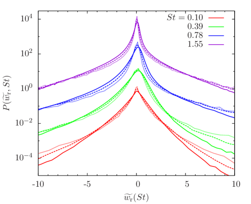
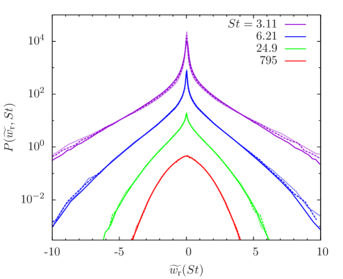
Figure 12.— The normalized PDF of the radial relative velocity, $w_{\rm r}$, as a function of the Stokes number $St$ and the particle distance, $r$. All PDFs are normalized to have unit variance. The normalized relative speed is defined as $\widetilde{w_{\rm r}}={w_{\rm r}}/\langle w_{\rm r}^{2}\rangle^{1/2}$. The solid, dashed and dotted lines correspond to particle distance $r=1,0.5$ and $0.25\eta$, respectively. The left panel plots the PDFs for particles with $St\leq 1.55$, while the right panel shows the results for larger particles with $St\geq 3.11$. In each panel, the bottom lines (i.e., $St=0.1$ and $St=795$) show the actual PDF values, and, for clarity, the upper lines for each larger $St$ are shifted upward by a factor of 16. One may change the normalization of the friction time using $\Omega=St/14.4$ and $\Omega_{\rm eddy}=St/19.2$.

6.2.3 The normalized PDF of the radial component

To see the shape of the PDF more clearly, we show in Fig. 12 the PDF of the radial component normalized to have unit variance. The radial relative speed is normalized to its rms value, $\langle w_{\rm r}^{2}\rangle^{1/2}$. The solid, dashed and dotted lines lines are the PDFs at $r=1\eta$, $0.5$ and $0.25\eta$, respectively, and the curves of different colors correspond to different $St$. The bottom curves in the left and right panels plot the actual PDF values for $St=0.1$ and $St=795$($\Omega=54$), respectively. For clarify, the PDF curves are shifted upward by a factor of 16 for each larger $St$ in the left panel or each smaller $St$ in the right panel. The asymmetry of the PDFs at $St\;\hbox to0.0pt{\lower 2.5pt\hbox{$\sim$}\hss}\raise 1.5pt\hbox{$<$}\;1.55$ is clearly seen.

As $St$ increases from 0.1 to 1.55, the central part of the normalized PDF $P(\widetilde{w_{\rm r}},St)$ becomes sharper. Before normalization, the innermost part of the PDF follows the PDF of the flow velocity difference, and is thus essentially the same for particles in the range $0.1\leq St\leq 1.55$ (see Fig. 10). Since the rms of $w_{\rm r}$ increases with $St$ due to the tail amplification, normalizing $w_{\rm r}$ by its rms tends to make the central part of the PDF sharper. At $St=3.11$ and $6.21$, the central cusp in the normalized PDF is very sharp. For $St$ above 3.11, the outer PDF parts become less fat with increasing $St$. The shape of the normalized PDF is helpful to understand the behavior of the ratio $\langle|w_{\rm r}|\rangle/\langle w_{\rm r}^{2}\rangle^{1/2}$ with $St$ discussed in §7.1.

It is interesting to note that, as $St$ increases from 0.1 to 0.39, the PDF, $P(\widetilde{w_{\rm r}},St)$, at small to intermediate $\widetilde{w_{\rm r}}$ in the right wing decreases. This corresponds to the decrease of $\langle w_{\rm r}^{2}\rangle_{+}^{1/2}$ in the $St$ range from 0.1 to 0.39 (see the left panel of Fig. 9). The physical reason is that the right wing corresponds to separating particle pairs, and the particle distance decreases toward the near past. This leads to a decrease in the primary distance, $r_{\rm p}$, for separating pairs with small to intermediate $\widetilde{w_{\rm r}}$, as $St$ increases from 0.1 to 0.39. For the far right tail with large $w_{\rm r}$, the particle pairs may quickly move past each other, and their distance starts to increase within a friction time in the past. This explains why the far right tail of $St=0.39$ particles becomes slightly broader than that for $St=0.1$. As $St$ increases to $0.78$, the PDF at immediate to large $\widetilde{w_{\rm r}}$ in the right wing is significantly amplified, while the effect of the “initial” decrease of the particle distance is still visible at small positive $\widetilde{w_{\rm r}}$. For $St>0.78$, the particle memory is longer, and the “initial” separation phase does not cause a significant difference in the primary distances $r_{\rm p}$ of separating and approaching particle pairs. The two wings become almost symmetric at $St\;\hbox to0.0pt{\lower 2.5pt\hbox{$\sim$}\hss}\raise 1.5pt\hbox{$>$}\;3.11$.

For particles with $St\;\hbox to0.0pt{\lower 2.5pt\hbox{$\sim$}\hss}\raise 1.5pt\hbox{$<$}\;3.11$, the normalized PDF has a dependence on the distance $r$ for the range of $r$ shown here. As $r$ decreases, the central part of the normalized PDF becomes sharper, and the outer parts become slightly broader, leading to a fatter PDF shape at smaller $r$. Before the normalization, the central part of the PDF follows the flow velocity difference at $r$, and its width thus decreases linearly with $r$. On the other hand, the dependence of the tails on $r$ is weaker because the primary distance, $r_{\rm p}$, for particle pairs in the outer parts of the PDF has a larger contribution from backward separation. Also, as $r$ decreases, the contribution from the outer parts of the PDF to the variance increases. Consequently, normalizing the PDF to unit variance gives a sharper central part and broader tails at smaller $r$. The fattening of the PDF with decreasing $r$ can also be viewed as due to the relatively larger contribution of caustics at the tails. The critical value $|w_{\rm r}^{\rm c}|$ decreases with decreasing $r$, suggesting that, for a given $St$, there are more caustic pairs at smaller $r$. We also observe that the asymmetry in the two wings decreases with decreasing $r$. However, it is remains to be verified whether it exactly disappears as $r\to 0$. At $St\;\hbox to0.0pt{\lower 2.5pt\hbox{$\sim$}\hss}\raise 1.5pt\hbox{$>$}\;12.4$, the PDF is essentially independent of $r$, and thus directly applicable for dust particle collisions. For these larger particles, $r_{\rm p}$ is mainly contributed by the backward separation even for pairs lying around the central part of the PDF, and thus the PDF is independent of $r$ for $w_{\rm r}$ in any range.

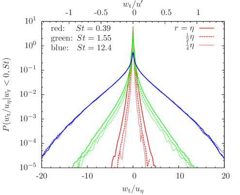
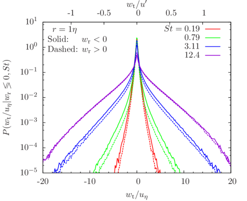
Figure 13.— Left panel: The PDF of tangential relative speed for approaching pairs at three distances for $St=0.39$, $1.55$ and $12.4$ particles. The PDF becomes independent of $r$ at $St\;\hbox to0.0pt{\lower 2.5pt\hbox{$\sim$}\hss}\raise 1.5pt\hbox{$>$}\;12.4$. Right panel: the tangential PDF for approaching ($w_{\rm r}<0$; solid) and separating ($w_{\rm r}>0$; dashed) particle pairs at $r=1\eta$. For $St<12.4$ particles, the PDF, $P(w_{\rm t}|w_{\rm r}<0$, St), of approaching pairs is wider than that of separating pairs ($w_{\rm r}>0$). Above $St=12.4$, the two conditional PDFs almost coincide.

6.2.4 The tangential PDFs: the $r$-dependence and approaching & separating pairs

The left panel of Fig. 13 shows the PDFs of the tangential relative speed at $r=1$, 0.5, and $0.25\eta$ for three values of $St$. At smaller $r$, the number of particle pairs available is smaller, leading to a decrease in the sample size. As a consequence, the PDFs become quite noisy at $r=\eta/4$, especially for small particles. For the $r$ range shown here, the PDF width decreases with decreasing $r$ for $St\;\hbox to0.0pt{\lower 2.5pt\hbox{$\sim$}\hss}\raise 1.5pt\hbox{$<$}\;6.21$ particles. The difference between the PDF tails at $\eta/4$ and $\eta/2$ appears to be smaller than that between $\eta/2$ and $\eta$, indicating relatively stronger contribution from caustic formation at smaller $r$. Like the radial PDF (Fig. 12), the PDF becomes independent of $r$ for $St\;\hbox to0.0pt{\lower 2.5pt\hbox{$\sim$}\hss}\raise 1.5pt\hbox{$>$}\;12.4$.

In the right panel of Fig. 13, we compare the PDFs of the tangential relative velocity for approaching ($P(w_{\rm t}|w_{\rm r}<0,St)$) and separating ($P(w_{\rm t}|w_{\rm r}>0,St)$) particle pairs at $r=1\eta$. For $St\;\hbox to0.0pt{\lower 2.5pt\hbox{$\sim$}\hss}\raise 1.5pt\hbox{$<$}\;6.2$, the PDF of approaching particles is broader than the separating ones, consistent with our earlier result for the rms relative speeds, $\langle w_{\rm t}^{2}\rangle^{1/2}_{\mp}$ (see the right panel of Fig. 9). Again, this is because, for a given “initial” value $r$, the distance of approaching particles was larger in the near past than the separating ones. Therefore, the PDF of the relative velocity for approaching pairs samples the PDF, $P_{\rm u}(\Delta u,\ell)$, of the flow difference at larger $\ell$. Since the width of $P_{\rm u}(\Delta u,\ell)$ increases with $\ell$, $P(w_{\rm t}|w_{\rm r}<0,St)$ is expected to be broader than $P(w_{\rm t}|w_{\rm r}>0,St)$. At $St\;\hbox to0.0pt{\lower 2.5pt\hbox{$\sim$}\hss}\raise 1.5pt\hbox{$>$}\;12.4$, the PDFs for approaching and separating pairs are almost equal. For these larger particles, the primary distance at $\tau\simeq-\tau_{\rm p}$ is insensitive to the initial conditions around $\tau=0$. Although $P(w_{\rm t}|w_{\rm r}>0,St)$ for separating particle pairs is not relevant for particle collisions, a comparison of $P(w_{\rm t}|w_{\rm r}<0,St)$ with $P(w_{\rm t}|w_{\rm r}>0,St)$ provides an interesting illustration for the role of the backward separation of particle pairs in determining their relative velocity.

6.2.5 The normalized PDF of the 3D amplitude

Fig. 14 plots the PDF of the 3D amplitude, $|{\boldsymbol{w}}|$, of the relative velocity for approaching particle pairs at $r=1\eta$. For each $St$, the amplitude $|{\boldsymbol{w}}|$ is normalized to the rms value $\langle w^{2}\rangle_{-}^{1/2}$, i.e., $\widetilde{|{\boldsymbol{w}}|}=|{\boldsymbol{w}}|/\langle w^{2}\rangle_{-}^{1/2}$, so that all the normalized PDFs have unit variance. The rms of the 3D amplitude, $\langle w^{2}\rangle_{-}^{1/2}$, for approaching pairs has been shown in Fig. 9. The left and right panels of Fig. 14 show simulation results for small ($St\leq 1.55$) and large ($St\geq 3.11$) particles, respectively. The thin dashed line in the left panel corresponds to approaching tracer particles ($St=0$), while the dashed line in right panel is the normalized PDF for a Gaussian vector with three independent components of equal variance. The PDF for tracer particles in the left panel is already highly non-Gaussian, as can be seen from a comparison with the dashed line in the right panel. In the left panel, the degree of non-Gaussianity increases as $St$ increases from $0$ to $\simeq 1$. At larger $St$, the PDF peaks at smaller $\widetilde{|{\boldsymbol{w}}|}$. The PDF around the rms value (i.e., $\widetilde{|{\boldsymbol{w}}|}\simeq 1$) decreases with increasing $St$, and more probability is distributed toward smaller and larger values of $\widetilde{|{\boldsymbol{w}}|}$. This corresponds to the sharpening of $P(w_{\rm r},St)$ and $P(w_{\rm t}|w_{\rm r}<0,St)$ in the central part and the broadening of the tail parts in this $St$ range (see Figs. 10, 11 and 12). The trend is reversed as $St$ increases further above $St\simeq 3.11$. The peak of the PDF moves back to around the rms value, $\widetilde{|{\boldsymbol{w}}|}\simeq 1$, at $St\;\hbox to0.0pt{\lower 2.5pt\hbox{$\sim$}\hss}\raise 1.5pt\hbox{$>$}\;49.7$ ($\Omega=3.5$). The PDF eventually approaches Gaussian in the limit $\tau_{\rm p}\gg T_{\rm L}$. However, note that, even for $St=795$ ($\Omega=54$) particles, the PDF shows a difference from the Gaussian distribution at small relative speeds.

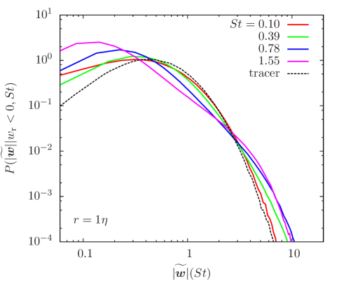
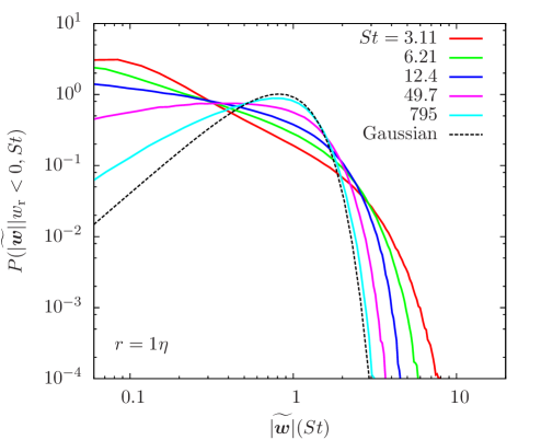
Figure 14.— The PDF of the 3D amplitude, $|{\boldsymbol{w}}|$, of the relative velocity for approaching particle pairs with $w_{\rm r}<0$. For each $St$, the amplitude, $|{\boldsymbol{w}}|$, is normalized to its rms value, and the PDF is normalized to have unit variance. In the left panel, the solid lines show results for $St\leq 1.55$, and the dashed line corresponds to the PDF for tracer particles ($St=0$). The right panel plots PDFs for $St\geq 3.11$. The dashed line in this panel is the normalized PDF, $\sqrt{\frac{54}{\pi}}\widetilde{|{\boldsymbol{w}}|}^{2}\exp(-3\widetilde{|{\boldsymbol{w}}|}^{2}/2)$, with unit variance for the amplitude of a Gaussian vector.

We find that, for $St$ in the range from 0.78 to 6.22, the PDF shows an extended power-law range at intermediate values of $\widetilde{|{\boldsymbol{w}}|}$. For example, at $St=0.78$, the PDF goes like $|{\boldsymbol{w}}|^{-2.4}$ in the range $0.5\leq\widetilde{|{\boldsymbol{w}}|}\leq 4$. The slope of the PDF in the power-law range becomes shallower with increasing $St$. For $St=1.55$, $St=3.11$ and $St=6.22$, the power-law exponent of the PDF in the intermediate $\widetilde{|{\boldsymbol{w}}|}$ range is $-1.8$, $-1.3$, and $-0.8$, respectively. The PDF of $|{\boldsymbol{w}}|$ can be easily computed from the PDFs of the radial and tangential components, if the three components are completely independent. In that case, one may obtain fitting functions for $P(|{\boldsymbol{w}}|)$ using the fitting functions discussed earlier for the PDFs, $P(w_{\rm r},St)$ and $P(w_{\rm t}|w_{\rm r}<0,St)$, of approaching particle pairs. One could also directly fit the PDF of $|{\boldsymbol{w}}|$ with simple function forms or tabulate it as a function of $St$. We will provide fitting functions for $P(|\boldsymbol{w}|,St)$ in a future paper.

The strong non-Gaussianity in the amplitude of the relative velocity has interesting implications for the growth and evolution of dust particles in planetary disks. We assume that the shape of the collision velocity PDF of dust particles at $r\to 0$ is more or less similar to the measured PDFs at $r\simeq\eta$ in our simulation, even though the PDFs of $St\;\hbox to0.0pt{\lower 2.5pt\hbox{$\sim$}\hss}\raise 1.5pt\hbox{$<$}\;12.4$ particles have not converged at $r\simeq\eta/4$. The shape of the PDFs shown in Fig. 14 suggests that there would more collisions with extremely large ($\widetilde{|{\boldsymbol{w}}|}\gg 1$) or small ($\widetilde{|{\boldsymbol{w}}|}\gg 1$) relative speeds than estimated from a Gaussian distribution. The higher probability for collisions with small relative speed would favor sticking, while there are also more collisions that would result in fragmentations. The competition of the two opposite effects would determine whether the non-Gaussian PDF of the collision velocity accelerates or slows down the particle growth. A coagulation model incorporating the non-Gaussian statistics of the collision speed would give a more realistic prediction for the evolution of the size distribution of dust particles.

7. The Collision Kernel

The prediction of the collision rate is one of the main goals of our study of the particle relative velocity. If the mean number density of inertial particles of a given size is $\bar{n}_{\rm p}$, the collision rate per unit volume between these identical particles is estimated by $\frac{1}{2}\bar{n}_{\rm p}^{2}\Gamma$, where $\Gamma$ is the collisional kernel and the factor 1/2 is used to avoid counting the same pair twice. Saffman and Turner (1956) presented two formulations for the collision kernel. The formulations were based on spherical and cylindrical geometries, respectively, and were thus named as the spherical and cylindrical formulations by Wang et al. (1998).

For the spherical formulation, we make use of the joint distribution, $\rho(r,w_{\rm r};St)$, of the particle distance and the radial relative speed, defined at the beginning of §6. The collision kernel for identical particles is written as (e.g., Saffman and Turner 1956),

$$\Gamma^{\rm sph}=-4\pi d_{\rm p}^{2}\int_{-\infty}^{0}\rho(d_{\rm p},w_{\rm r};St)w_{\rm r}dw_{\rm r}$$ (37)

where $d_{\rm p}$ is the diameter of the particle, and the integral limits include only particle pairs moving toward each other. Using the definition of the radial PDF, $P(w_{\rm r},St)$ as $\rho(r,w_{\rm r};St)/g(r,St)$, eq. (37) can be expressed in a simpler form, $\Gamma^{\rm sph}=4\pi d_{\rm p}^{2}g(r,St)F_{\rm r}^{-}$, where $F_{\rm r}$ is the inward flux of particles toward a given reference particle defined as $F_{\rm r}^{-}=-\int_{-\infty}^{0}w_{\rm r}P(w_{\rm r},St)dw_{\rm r}$.

The particle statistics become stationary when the dynamics is fully relaxed. In the steady state, the inward flux, $F_{\rm r}^{-}$, is equal to the outward flux $F^{+}$($\equiv\int_{0}^{\infty}w_{\rm r}P(w_{\rm r},St)dw_{\rm r}$) (Wang et al. 2000), which is confirmed by our simulation data. This is because the average radial velocity $\langle w_{\rm r}\rangle=0$, as expected from statistical isotropy, and $\langle w_{\rm r}\rangle=F_{\rm r}^{+}-F_{\rm r}^{-}$ by definition. We thus have $F_{\rm r}^{+}=F_{\rm r}^{-}=\frac{1}{2}\langle|w_{\rm r}|\rangle$ where $\langle|w_{\rm r}|\rangle$ is the ensemble average of the absolute value of the radial relative velocity. The collision kernel can then be written as (Wang et al. 2000),

$$\Gamma^{\rm sph}=2\pi d_{\rm p}^{2}g(d_{\rm p},St)\langle|w_{\rm r}|\rangle.$$ (38)

The cylindrical formulation assumes that all particles inside a cylinder of length $\langle|{\boldsymbol{w}}|\rangle dt$ located at a distance $d_{\rm p}$ from a given particle will collide with the particle in a time interval $dt$. Similar to eq. (38), the cylindrical collision kernel can be written as $\Gamma^{\rm cyl}=\pi d_{\rm p}^{2}g\langle|{\boldsymbol{w}}|\rangle$, with $\langle|{\boldsymbol{w}}|\rangle$ being the average of the 3D amplitude of the relative velocity.

To evaluate the collision kernel, one can start directly from eq. (37) using the joint distribution, $\rho(r,w_{\rm r};St)$. However, previous studies have shown that considering the RDF and $\langle|w_{\rm r}|\rangle$ separately provides interesting insights on the estimate of the particle collision rate (e.g., Sundaram & Collins 1997, Wang et al. 2000). In §7.1, we compute the RDF and the absolute average of the relative speed from our simulation data.

7.1. The Overall RDF and Absolute Average of the Relative Speed

The RDF represents the probability of finding a neighboring particle at a distance of $r$ with any relative velocity, and is a measure for the spatial clustering of the particles. Due to their finite inertia, inertial particles do not exactly follow the flow velocity and have been found to exhibit inhomogeneous distribution even in incompressible turbulence. Turbulent clustering of inertial particles has been extensively investigated in the literature (see e.g., Maxey 1987, Sundaram and Collins 1997, Wang et al. 2000, Cuzzi et al. 2001, Hogan & Cuzzi 2001, Balkovsky et al. 2001, Zaichik et al. 2003, Falkovich and Pumir 2004, Cuzzi et al. 2008, Pan et al. 2011). The general physical interpretation for turbulent clustering is that vortical structures in turbulent flows tend to expel inertial particles. The particles are pushed out of high-vorticity regions by the centrifugal force, leading to the formation of clusters in strain-dominated regions.

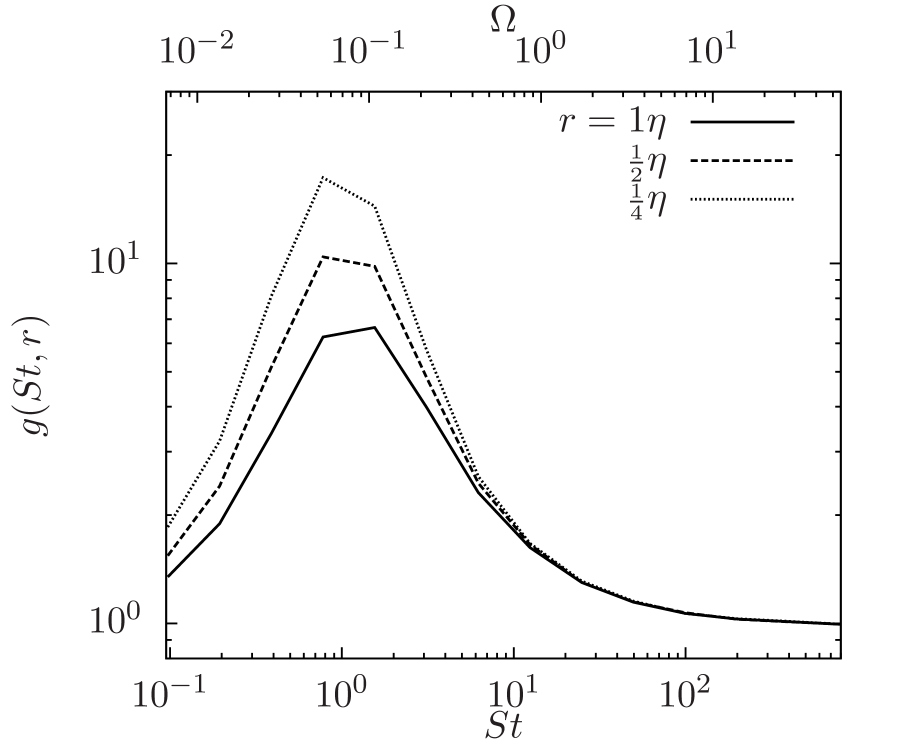
Figure 15.— The radial distribution function, $g(St,r)$, as a function of the Stokes number at $r=1$ (solid), $0.5$ (dashed) and $0.25\eta$ (dotted).

Fig. 15 plots the RDF as a function of $St$ at $r=1$, 0.5 and $0.25\eta$. Consistent with previous studies, the RDF is largest for $St\simeq 1$ particles, whose friction timescale couples with the smallest scale of the turbulent flow. For $r$ in the dissipation rage, the RDF increases toward smaller $r$ as a power-law, i.e., $g(St,r)\propto r^{-\mu}$. The scaling exponent $\mu$ peaks at $St\simeq 1$, and approaches zero in the limits $St\ll 1$ and $St\gg 1$. We measured $\mu$ using the values of $r$ shown in Fig. 15, and found that $\mu=0.73$ for $St=0.78$, consistent with the result of Pan et al. (2011). The interested reader is referred to Pan et al. (2011) for the scaling exponent, $\mu$, as a function of $St$.

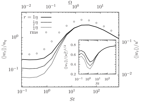
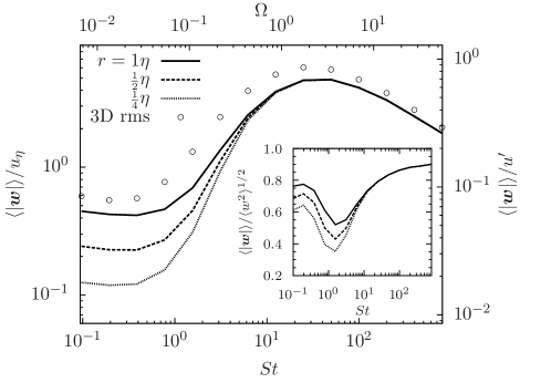
Figure 16.— Left panel: The average of the absolute value of the radial relative speed, $\langle|w_{\rm r}|\rangle$, as a function of the Stokes number. Solid, dashed and dotted lines correspond to the particle distance $r=1,0.5$ and $0.25\eta$, respectively. For comparison, the circles show the rms, $\langle w_{\rm r}^{2}\rangle^{1/2}$, of the radial relative speed at $r=1\eta$. The inset plots the ratio, $\langle|w_{\rm r}|\rangle/\langle w_{\rm r}^{2}\rangle^{1/2}$, at $r=1$ (solid), $0.5$ (dashed) and $0.25\eta$ (dotted). Right panel: same as the left panel, but for the 3D amplitude, $|{\boldsymbol{w}}|$, and the 3D rms, $\langle w^{2}\rangle^{1/2}$, of the relative velocity.

In the left panel of Fig. (16), we plot the simulation result for $\langle|w_{\rm r}|\rangle$ at $r=1,0.5$, and $0.25\eta$. For comparison, we also show the data (circles) for the rms of the radial relative speed at $r=1\eta$. Qualitatively, $\langle|w_{\rm r}|\rangle$ as a function of $St$ and $r$ is similar to the rms. It is smaller than the rms, as it corresponds to the 1st-order moment of the PDF, $P(w_{\rm r},St)$, of $w_{\rm r}$. Most theoretical models, including our own, for the particle relative velocity are based on the computation of the variance (e.g., $\langle w_{\rm r}^{2}\rangle$), and cannot be directly applied to predict $\langle|w_{\rm r}|\rangle$. The conversion between $\langle w_{\rm r}^{2}\rangle$ and $\langle|w_{\rm r}|\rangle$ relies on the shape of the PDF of $w_{\rm r}$, which is difficult to predict. We thus did not attempt to fit $\langle|w_{\rm r}|\rangle$ with a model prediction.

Similar to the S-T formula (eq. 11) for the variances of the relative velocity, we would predict that $\langle|w_{\rm r}|\rangle=\langle|\Delta u_{\rm r}|\rangle$ in the $St\ll 1$ limit, where $\langle|\Delta u_{\rm r}|\rangle$ is the absolute average of the longitudinal flow velocity increment. At $\ell\;\hbox to0.0pt{\lower 2.5pt\hbox{$\sim$}\hss}\raise 1.5pt\hbox{$<$}\;\eta$, $\langle|\Delta u_{\rm r}|\rangle$ is expected to scale linearly with $\ell$. We find that, for $St\ll 1$, $\langle|w_{\rm r}|\rangle\propto r^{0.9}$, which is slightly shallower than the linear scaling. This is likely caused by the contribution from the effect of slings or caustics. The scaling is steeper than $r^{0.78}$ for the radial rms velocity (see §6.1.2), suggesting that $\langle|w_{\rm r}|\rangle$ follows the flow velocity scaling better. The behavior of $\langle|\Delta u_{\rm r}|\rangle$ at small $St$ also appears to be more regular than that of $\langle w_{\rm r}^{2}\rangle^{1/2}$. For all three values of $r$, the $\langle|w_{\rm r}|\rangle$ curves become flat at $St\;\hbox to0.0pt{\lower 2.5pt\hbox{$\sim$}\hss}\raise 1.5pt\hbox{$<$}\;0.4$. The likely reason is that $\langle|w_{\rm r}|\rangle$ represents statistics at a lower order than the variance (or rms), and is thus less affected by the rare and extreme sling events, or by the numerical uncertainty in the particle trajectory computation.

The inset of the left panel shows the ratio of the absolute average to the rms. The ratio depends on the PDF shape of $w_{\rm r}$, and particularly on the central part of the PDF because both $\langle|w_{\rm r}|\rangle$ and the rms are lower-order moments. As a reference, if the PDF $P(w_{\rm r},St)$ is Gaussian, we have $\langle|w_{\rm r}|\rangle/\langle w_{\rm r}^{2}\rangle^{1/2}=(2/\pi)^{1/2}=0.80$ (e.g., Wang et al. 2000), and for an exponential PDF it is equal to $1/\sqrt{2}$. The ratio from a Gaussian PDF was usually used to convert the model predictions for the rms to $\langle|w_{\rm r}|\rangle$ (Wang et al. 2000, Zaichik et al. 2003, 2006). Generally, the ratio is smaller if the central PDF is sharper and the tails are fatter. As seen in the inset, the ratio reaches a minimum at $St\simeq 1$, corresponding to a maximum fatness of the PDF at $St\simeq 1$ (see §6.2.3). At $r\leq\eta$, the minimum is smaller than 0.45, corresponding to highly non-Gaussian PDF. At $St\simeq 800$, $\langle|w_{\rm r}|\rangle/\langle w_{\rm r}^{2}\rangle^{1/2}$ reaches 0.78, close to the expected value for a Gaussian PDF. For the range of $r$ shown here, the ratio also decreases with decreasing $r$ for $St\;\hbox to0.0pt{\lower 2.5pt\hbox{$\sim$}\hss}\raise 1.5pt\hbox{$<$}\;6$, which is expected from the trend of the PDF shape with $r$ for these particles (§6.2.3).

Our simulation result for $\langle|{\boldsymbol{w}}|\rangle$ is shown in the right panel of Fig. (16), which is very similar to the left panel for $\langle|w_{\rm r}|\rangle$. At $St\;\hbox to0.0pt{\lower 2.5pt\hbox{$\sim$}\hss}\raise 1.5pt\hbox{$<$}\;0.4$, we find $\langle|{\boldsymbol{w}}|\rangle$ also scales as $r^{0.9}$ with $r$. The ratio of $\langle|{\boldsymbol{w}}|\rangle$ to $\langle w^{2}\rangle^{1/2}$ also shows a dip at $St\simeq 1$. The ratio approaches 0.9 at the largest $St$, as expected from a 3D Gaussian distribution.

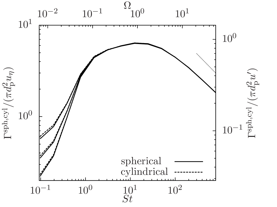
Figure 17.— The collision kernels normalized to $\pi d_{\rm p}^{2}u_{\eta}$. The solid lines plot $2g(St,r)\langle|w_{\rm r}|\rangle/u_{\eta}$ for the spherical formulation, and the dashed lines show $g(St,r)\langle|{\boldsymbol{w}}|\rangle/u_{\eta}$ for the cylindrical formulation. The lines from bottom to top correspond to normalized kernels measured at $r=0.25$, $0.5$ and $1\eta$, respectively. The dotted line segment corresponds to a $St^{-1/2}$ scaling.

In Fig. 17, we plot $\Gamma^{\rm sph}$ and $\Gamma^{\rm cyl}$ normalized to $\pi d_{\rm p}^{2}u_{\eta}$. The normalized kernels correspond to the product $2g(St,r)\langle|w_{\rm r}|\rangle/u_{\eta}$ (solid lines) for the spherical formulation and $g(St,r)\langle|{\boldsymbol{w}}|\rangle/u_{\eta}$ (dashed lines) for the cylindrical formulation. We will also refer to these products as the collision kernel per unit cross section. At each $r$, the solid and dashed lines almost coincide, meaning that $\Gamma^{\rm sph}$ and $\Gamma^{\rm cyl}$ are nearly equal at all $St$ and $r$. This suggests that $\langle|w_{\rm r}|\rangle\simeq 0.5\langle|{\boldsymbol{w}}|\rangle$ since $\Gamma^{\rm sph}/\Gamma^{\rm cyl}=2\langle|w_{\rm r}|\rangle/\langle|{\boldsymbol{w}}|\rangle$. The two collision kernels have a noticeable difference only at $St=0.1-0.2$, where $\Gamma^{\rm sph}$ is smaller than $\Gamma^{\rm cyl}$ by $\;\hbox to0.0pt{\lower 2.5pt\hbox{$\sim$}\hss}\raise 1.5pt\hbox{$<$}\;5\%$. This is consistent with the result of Wang et al. (2000). Wang et al. (2000) also showed that the spherical formulation provides an almost exact description for the particle collision rate. The near equality of $\Gamma^{\rm sph}$ and $\Gamma^{\rm cyl}$ at all $St$ and $r$ suggests that one can apply either formulation to evaluate the collision rate.

Fig. 17 shows that $2g(St,r)\langle|w_{\rm r}|\rangle$ and $g(St,r)\langle|{\boldsymbol{w}}|\rangle$ are independent of $r$ for $St\geq 1$. Apparently, this is because, at $St\;\hbox to0.0pt{\lower 2.5pt\hbox{$\sim$}\hss}\raise 1.5pt\hbox{$>$}\;1$, the $r$-dependences of the RDF $g(St,r)$ and the absolute average $\langle|w_{\rm r}|\rangle$ (or $\langle|{\boldsymbol{w}}|\rangle$) almost cancel out (see Figs. 15 and 16). A more interesting perspective is that the inverse scaling of $g(St,r)$ and $\langle|w_{\rm r}|\rangle$ is expected from the intuition that the normalized kernel approaches a finite constant, corresponding to a finite collision rate, at sufficiently small $r$. Therefore, the scalings of $g(St,r)$ and $\langle|w_{\rm r}|\rangle$ must cancel out once the kernel converges (see more discussions in §7.2). At $St=1.55$, $g(St,r)$ increases with decreasing $r$ as $\propto r^{-0.55}$, while both $\langle|w_{\rm r}|\rangle$ and $\langle|{\boldsymbol{w}}|\rangle$ scale with $r$ as $\propto r^{0.57}$. Note that, if the $r^{0.57}$ scaling of the relative speed persists in the $r\to 0$ limit, it does mean the collision energy is zero for nearly-point particles. This is because $\langle|w_{\rm r}|\rangle$ or $\langle|{\boldsymbol{w}}|\rangle$ does not represent the collision energy. The average collision energy per collision is expected to be finite even if $\langle|w_{\rm r}|\rangle$ or $\langle|{\boldsymbol{w}}|\rangle$ approaches zero at $r\to 0$ (see §7.2). The cancellation between the overall $g(St,r)$ and $\langle|w_{\rm r}|\rangle$ for $St\;\hbox to0.0pt{\lower 2.5pt\hbox{$\sim$}\hss}\raise 1.5pt\hbox{$>$}\;1$ particles needs to be interpreted with care. As discussed in §6.2, at a given $r$, there are two types of particle pairs, i.e., continuous and caustic pairs. The two types have different properties, and the inverse scalings of the overall RDF and relative velocity could be an artifact of not properly splitting the two types of particle pairs. In §7.2, we will evaluate the contribution from each type of pairs.

We find that the collision kernel per unit cross section shows an abrupt increase as $St$ increases toward 1 (see, e.g., Sundaram & Collins 1997), increases only slightly for $St$ between $1$ and $St_{\rm m}\simeq 30$, and starts to decrease at $St\simeq 30$. It finally scales with $St$ as $St^{-1/2}$ at $\tau_{\rm p}\gg T_{\rm L}$. A physical discussion for the behaviors is given in §7.2.

The $r-$independence of the kernel of $St\geq 1$ particles at $r\simeq\eta$ implies that one may apply our result to estimate the collision kernel of $St\;\hbox to0.0pt{\lower 2.5pt\hbox{$\sim$}\hss}\raise 1.5pt\hbox{$>$}\;1$ dust particles in protoplanetary turbulence, even though the dust particle diameter $d_{\rm p}$ is smaller than $\eta$ by orders of magnitude. On the other hand, at $St\;\hbox to0.0pt{\lower 2.5pt\hbox{$\sim$}\hss}\raise 1.5pt\hbox{$<$}\;1$, the measured collision kernel depends on $r$ in the range of $r$ considered, and is thus not directly applicable for dust particles with $St\;\hbox to0.0pt{\lower 2.5pt\hbox{$\sim$}\hss}\raise 1.5pt\hbox{$<$}\;1$. To achieve a general understanding of the $r\to 0$ limit, it would be useful if one could isolate an $r$-independent contribution. For this purpose, we make a preliminary attempt to separate the contributions from the continuous and caustic pairs.

7.2. Decomposing the Continuous and Caustic Contributions

As discussed in §6.2, at a given distance, $r$, there are two types of particle pairs, corresponding to the continuous (inner) and caustic (tail) parts of the relative velocity PDF. For the radial relative speed PDF of approaching particle pairs, the two parts can be roughly divided by a critical value, $w_{\rm r}^{\rm c}\simeq-r/\tau_{\rm p}$. In this section, we separate the contributions of the two types of pairs to the collision kernel in the spherical formulation. Using the relation $\rho(r,w_{\rm r};St)=g(r,St)P(w_{\rm r},St)$, and splitting the left wing of $P(w_{\rm r},St)$ into two parts, the collision kernel, eq. (37), is written as,

$$\Gamma^{\rm sph}=\Gamma^{\rm con}+\Gamma^{\rm cau},$$ (39)

where $\Gamma^{\rm con}=-4\pi d_{\rm p}^{2}g(r,St)\int_{w_{\rm r}^{\rm c}}^{0}w_{\rm r}P(w_{\rm r},St)dw_{\rm r}$ and $\Gamma^{\rm cau}=-4\pi d_{\rm p}^{2}g(r,St)\int_{-\infty}^{w_{\rm r}^{\rm c}}w_{\rm r}P(w_{\rm r},St)dw_{\rm r}$. The continuous and caustic contributions can be expressed in more convenient forms,

$$\Gamma^{\rm con}=4\pi d_{\rm p}^{2}g^{\rm con}\langle w_{\rm r}^{\rm con}\rangle$$

$$\Gamma^{\rm cau}=4\pi d_{\rm p}^{2}g^{\rm cau}\langle w_{\rm r}^{\rm cau}\rangle$$ (40)

where $g^{\rm con}(r,St)\equiv g(r,St)\int_{w_{\rm r}^{\rm c}}^{0}P(w_{\rm r},St)dw_{\rm r}$ and $g^{\rm cau}(r,St)\equiv g(r,St)\int_{-\infty}^{w_{\rm r}^{\rm c}}P(w_{\rm r},St)dw_{\rm r}$ are the RDFs of continuous and caustic pairs, corresponding to the probabilities of finding an approaching neighbor that makes a continuous and caustic pair, respectively. The sum of $g^{\rm con}$ and $g^{\rm cau}$ is given by $g^{-}\equiv g(r,St)\int_{-\infty}^{0}P(w_{\rm r},St)dw_{\rm r}$. Because there are more separating pairs than approaching ones, $g^{-}$ is smaller (by 10-20%) than $0.5g(r,St)$ at $St\;\hbox to0.0pt{\lower 2.5pt\hbox{$\sim$}\hss}\raise 1.5pt\hbox{$<$}\;10$. It becomes equal to $0.5g$ at $St\;\hbox to0.0pt{\lower 2.5pt\hbox{$\sim$}\hss}\raise 1.5pt\hbox{$>$}\;10$. The average radial relative speeds for the two types of pairs are defined as $\langle w_{\rm r}^{\rm con}\rangle=-\int_{w_{\rm r}^{\rm c}}^{0}w_{\rm r}P(w_{\rm r},St)dw_{\rm r}/\int_{w_{\rm r}^{\rm c}}^{0}P(w_{\rm r},St)dw_{\rm r}$, and $\langle w_{\rm r}^{\rm cau}\rangle=-\int_{-\infty}^{w_{\rm r}^{\rm c}}w_{\rm r}P(w_{\rm r},St)dw_{\rm r}/\int_{-\infty}^{w_{\rm r}^{\rm c}}P(w_{\rm r},St)dw_{\rm r}$. The four quantities, $g^{\rm con}$, $g^{\rm cau}$, $\langle w_{\rm r}^{\rm con}\rangle$, and $\langle w_{\rm r}^{\rm cau}\rangle$, depend on $w_{\rm r}^{\rm c}$, whose exact value is uncertain. We will set $w_{\rm r}^{\rm c}=-r/\tau_{\rm p}$ here, and defer a study on the effect of the choice of $w_{\rm r}^{\rm c}$ to a later work.

In the formulation of Falkovich et al. (2002) for the collision kernel of $St\;\hbox to0.0pt{\lower 2.5pt\hbox{$\sim$}\hss}\raise 1.5pt\hbox{$<$}\;1$ particles, the clustering effect enters only for the S-T (continuous) contribution. The RDF was theoretically modeled and evaluated by considering the continuous-type particles only. For the continuous pairs, $\langle w_{\rm r}^{\rm con}\rangle$ scales linearly with $r$, as in the S-T prediction. The continuous contribution to the kernel is amplified by the clustering effect. On the other hand, the Falkovich et al. formulation suggests that clustering plays no role for the sling (caustic) contribution. Both $\langle w_{\rm r}^{\rm cau}\rangle$, and the normalized kernel $\Gamma^{\rm cau}/(\pi d_{\rm p}^{2})$ due to the slings are independent of the particle distance (Falkovich et al. 2002). These also imply that $g^{\rm cau}$ is $r$-independent. The model of Gustavsson & Mehlig (2011) provides a similar formulation for the collision kernel. The continuous contribution is essentially the same as that in Falkovich et al. (2002). They also predicted an $r$-independent caustic contribution to the normalized kernel. However, unlike Falkovich et al. (2002), their derivation accounts for the possibility that both $g^{\rm cau}$ and $\langle w_{\rm r}^{\rm cau}\rangle$ may depend on $r$. But their scaling exponents exactly cancel out, giving an $r$-independent contribution to the kernel.

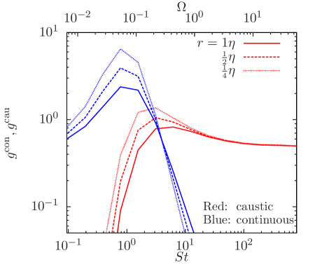
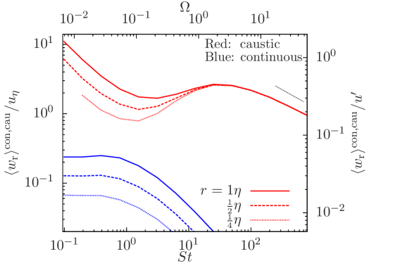
Figure 18.— Left panel: RDFs for continuous (blue) and caustic (red) particle pairs at $r=1\eta$ (solid), 0.5 $\eta$ (dashed) and 0.25 $\eta$ (dotted), respectively. Right panel: Average velocities, $\langle w_{\rm r}^{\rm con}\rangle$ and $\langle w_{\rm r}^{\rm cau}\rangle$, of continuous and caustic pairs at the same three distances. The dotted line segment denotes a $St^{1/2}$ scaling. In both panels, the critical value, $w_{\rm r}^{\rm c}$, is set to $-r/\tau_{\rm p}$. The red dotted-curve in the right panel lacks a point at $St=0.1$ because no caustic pairs were found for $St=0.1$ particles at $r=\eta/4$ in the simulation. For the corresponding curve in the left panel, $g^{\rm cau}$ drops to zero at $St=0.1$, which is not visible due to the selected Y-range in the figure.

In the left panel of Fig. 18, we plot $g^{\rm con}$ (blue) and $g^{\rm cau}$ (red) computed from our simulation data at three distances. At $St\;\hbox to0.0pt{\lower 2.5pt\hbox{$\sim$}\hss}\raise 1.5pt\hbox{$<$}\;1$, the number of caustic pairs is small, and most particle pairs belong to the continuous type. The continuous-type particles show significant clustering at $St\;\hbox to0.0pt{\lower 2.5pt\hbox{$\sim$}\hss}\raise 1.5pt\hbox{$<$}\;3$, and the RDF $g^{\rm con}$ increases toward smaller $r$ with similar scaling exponents as the overall RDF. These suggest that the origin of strong clustering at $St\;\hbox to0.0pt{\lower 2.5pt\hbox{$\sim$}\hss}\raise 1.5pt\hbox{$<$}\;3$ corresponds to the continuous-type particles (Falkovich et al. 2002). Similar to the overall RDF (Fig. 15), $g^{\rm con}$ peaks at $St\simeq 1$. At larger $St$, $g^{\rm con}$ decreases rapidly with $St$, and becomes comparable to $g^{\rm cau}$ at $St\simeq 3$. The fast drop of $g^{\rm con}$ at $St\;\hbox to0.0pt{\lower 2.5pt\hbox{$\sim$}\hss}\raise 1.5pt\hbox{$>$}\;3$ is because it becomes sensitive to the critical value, $w_{\rm r}^{\rm c}$, as the range $(w_{\rm r}^{\rm c},0)$ narrows with increasing $St$. This range also becomes narrower with decreasing $r$, and this causes $g^{\rm con}$ to slightly decease with decreasing $r$ at $St\;\hbox to0.0pt{\lower 2.5pt\hbox{$\sim$}\hss}\raise 1.5pt\hbox{$>$}\;3$. At $St\simeq 6.2$, $g^{\rm con}$ is significantly smaller than $g^{\rm cau}$, and essentially all particle pairs are of the caustic type. The caustic RDF $g^{\rm cau}$ increases with decreasing $r$ for particles with $St\;\hbox to0.0pt{\lower 2.5pt\hbox{$\sim$}\hss}\raise 1.5pt\hbox{$<$}\;10$, and is $r$-independent at larger $St$.

Concerning the $r$-dependence of $g^{\rm cau}$ at $St\;\hbox to0.0pt{\lower 2.5pt\hbox{$\sim$}\hss}\raise 1.5pt\hbox{$<$}\;10$, there are several possibilities. The first is that this dependence is generic, and $g^{\rm cau}\to\infty$ as $r\to 0$, as considered by Gustavsson & Mehlig (2011). Second, the $r$-dependence of $g^{\rm cau}$ may disappear at sufficiently small $r$, and $g^{\rm cau}$ finally converges to a finite constant, as assumed in Falkovich et al. (2002). In this case, one may in principle achieve a converged $g^{\rm cau}$ by using a larger number of $St\;\hbox to0.0pt{\lower 2.5pt\hbox{$\sim$}\hss}\raise 1.5pt\hbox{$<$}\;10$ particles in the simulation to resolve smaller scales. We checked $r=\eta/8$ in our simulation and found that the convergence is not reached yet. Third, the $r$-dependence of $g^{\rm cau}$ may be an artifact of our selected value for $w_{\rm r}^{\rm c}$. We attempted to vary $w_{\rm r}^{\rm c}$ around $-r/\tau_{\rm p}$ by a factor 4, but were not able to find a considerable decrease in the $r$-dependence of $g^{\rm cau}$. It is also possible that the transition from the continuous to the caustic type is gradual, and thus exactly splitting two types by a single critical value ($w_{\rm r}^{\rm c}$) is impossible at least at the scales explored here. We note that $g^{\rm cau}$ is larger than 0.5 at $St\simeq 3.11$, suggesting some degree of clustering for caustic-type particles. This, however, could be an artifact that the two types of pairs are not split precisely.

The right panel of Fig. 18 shows the average relative speeds, $\langle w_{\rm r}^{\rm con}\rangle$ and $\langle w_{\rm r}^{\rm cau}\rangle$, for continuous (blue) and caustic (red) pairs. At $St\ll 1$, $\langle w_{\rm r}^{\rm con}\rangle$ is constant with $St$ and decreases linearly with $r$, as in the S-T prediction. At $St\;\hbox to0.0pt{\lower 2.5pt\hbox{$\sim$}\hss}\raise 1.5pt\hbox{$>$}\;1$, $\langle w_{\rm r}^{\rm con}\rangle$ decreases with $St$. This is because the number of continuous pairs becomes small and the average relative speed starts to have a sensitive dependence on the lower limit $w_{\rm r}^{\rm c}$, which becomes closer to zero as $St$ increases. By definition, the caustic pairs have larger relative velocity than continuous pairs. At $St\ll 1$, the sling events or caustic formation occur only in regions with very large velocity gradient, and this is responsible for the large relative velocity for caustic pairs at small $St$. As $St$ increases, the criterion for the sling events to occur becomes weaker, as reflected by the decrease of $|w_{\rm r}^{\rm c}|$. This results in a decrease in $\langle w_{\rm r}^{\rm cau}\rangle$ toward $St\simeq 1$. At $St\;\hbox to0.0pt{\lower 2.5pt\hbox{$\sim$}\hss}\raise 1.5pt\hbox{$>$}\;3$, most particles belong to the caustic type, and thus the trend of $\langle w_{\rm r}^{\rm cau}\rangle$ as a function $St$ becomes similar to the overall relative speed $\langle|w_{\rm r}|\rangle$ (see Fig. 16). It first increases with $St$ for $3\;\hbox to0.0pt{\lower 2.5pt\hbox{$\sim$}\hss}\raise 1.5pt\hbox{$<$}\;St\;\hbox to0.0pt{\lower 2.5pt\hbox{$\sim$}\hss}\raise 1.5pt\hbox{$<$}\;St_{\rm m}\simeq 30$, and then decreases at $St\;\hbox to0.0pt{\lower 2.5pt\hbox{$\sim$}\hss}\raise 1.5pt\hbox{$>$}\;St_{\rm m}$. At the three distances shown here, $\langle w_{\rm r}^{\rm cau}\rangle$ decreases with decreasing $r$ for $St\;\hbox to0.0pt{\lower 2.5pt\hbox{$\sim$}\hss}\raise 1.5pt\hbox{$<$}\;10$ particles, as the condition to have a caustic pair is weaker at smaller $r$. Again, the $r$-dependence of $\langle w_{\rm r}^{\rm cau}\rangle$ may disappear at much smaller $r$ and/or with a better method to split the two types of pairs. At $St\;\hbox to0.0pt{\lower 2.5pt\hbox{$\sim$}\hss}\raise 1.5pt\hbox{$>$}\;10$, both $g^{\rm cau}$ and $\langle w_{\rm r}^{\rm cau}\rangle$ are independent of $r$, indicating full resolution of their statistics in our simulation.

In Fig. 19, we show the continuous (blue) and caustic (red) contributions to the collision kernel per unit cross section. In the $r$ range shown here, the continuous and caustic contributions dominate for $St\;\hbox to0.0pt{\lower 2.5pt\hbox{$\sim$}\hss}\raise 1.5pt\hbox{$<$}\;1$ and $St\;\hbox to0.0pt{\lower 2.5pt\hbox{$\sim$}\hss}\raise 1.5pt\hbox{$>$}\;1$, respectively. The continuous contribution decreases with $r$, corresponding to the $r$-dependence of the overall kernel, $\Gamma^{\rm sph}$, in Fig. 17. The decrease of the continuous contribution with $r$ is expected from the scaling exponents of $g^{\rm con}$ and $\langle w^{\rm con}\rangle$. With decreasing $r$, $\langle w^{\rm con}\rangle$ decreases linearly, which is faster than the increase of $g^{\rm con}$. In the limit $r\to 0$, the continuous contribution is expected to vanish for all particles. This means that, although amplified by clustering, the continuous-type particles do not significantly contribute to the collision rate of dust particles, as pointed out by Hubbard (2012).

The contribution of the caustic-type particles to the normalized kernel is found to be approximately $r$-independent. The differences in three red lines are small, and one may claim achieving numerical convergence at $r=\eta/4$ for all particles. The $r$-independence of $\Gamma^{\rm cau}/(\pi r_{\rm p}^{2})$ for $St\;\hbox to0.0pt{\lower 2.5pt\hbox{$\sim$}\hss}\raise 1.5pt\hbox{$<$}\;10$ particles at the distances explored here is related to the cancellation of the scalings of $g^{\rm cau}$ and $\langle w_{\rm r}^{\rm cau}\rangle$. Intuitively, one would expect that the collision rate of inertial particles converges to a finite constant in the $r\to 0$ limit. Therefore, $g^{\rm cau}$ and $\langle w_{\rm r}^{\rm cau}\rangle$ must have inverse scalings with $r$, once the caustic kernel converges. On the other hand, one may prove the intuition of a finite constant caustic kernel at sufficiently small $r$ by showing that $g^{\rm cau}$ and $\langle w_{\rm r}^{\rm cau}\rangle$ scale inversely with $r$, which was actually predicted by the theoretical model of Gustavsson & Mehlig (2011). As discussed earlier, both $g^{\rm cau}$ and $\langle w_{\rm r}^{\rm cau}\rangle$ may become independent of $r$ at much smaller $r$. However, it is also possible that, as $r\to 0$, $g^{\rm cau}\to\infty$ and $\langle w_{\rm r}^{\rm cau}\rangle\to 0$, especially for $St\;\hbox to0.0pt{\lower 2.5pt\hbox{$\sim$}\hss}\raise 1.5pt\hbox{$<$}\;1$ particles. Note that $\langle w_{\rm r}^{\rm cau}\rangle$ does not represent the collisional energy at all. Even if $\langle w_{\rm r}^{\rm cau}\rangle\to 0$, it does not suggest the average collisional energy is zero. In fact, a computation of the average collision energy per collision (i.e., the relative velocity variance weighted by the collision rate; see, e.g., Hubbard 2012) by caustic pairs for particles with $1\;\hbox to0.0pt{\lower 2.5pt\hbox{$\sim$}\hss}\raise 1.5pt\hbox{$<$}\;St\;\hbox to0.0pt{\lower 2.5pt\hbox{$\sim$}\hss}\raise 1.5pt\hbox{$<$}\;10$ in our simulation shows that it already converges to a finite constant at $r=\eta/4$. The collision energy (velocity) of $St\;\hbox to0.0pt{\lower 2.5pt\hbox{$\sim$}\hss}\raise 1.5pt\hbox{$<$}\;10$ particles by caustic pairs in the $r\to 0$ limit will be examined systematically in a future study.

The $r$-independence of the caustic contribution is responsible for that of the overall normalized kernel at $St\;\hbox to0.0pt{\lower 2.5pt\hbox{$\sim$}\hss}\raise 1.5pt\hbox{$>$}\;1$ observed in Fig. 17. Because the continuous contribution vanishes as $r\to 0$, and due to the convergence of the caustic contribution, one may use our result for $\Gamma^{\rm cau}$ to estimate the collision rate of nearly point-like dust particles. One caveat, however, is that $\Gamma^{\rm cau}$ has a dependence on the critical value, $w_{\rm r}^{\rm c}$, for $St\;\hbox to0.0pt{\lower 2.5pt\hbox{$\sim$}\hss}\raise 1.5pt\hbox{$<$}\;1$ particles, an issue that will be refined in a future work.

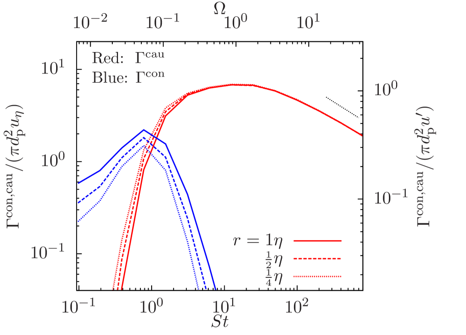
Figure 19.— The continuous ($\Gamma^{\rm con}$; blue) and caustic ($\Gamma^{\rm cau}$; red) contributions to the kernel normalized to $\pi d_{\rm p}^{2}u_{\eta}$ or $\pi d_{\rm p}^{2}u^{\prime}$ on the left and right Y-axis, respectively. The solid, dashed and dotted lines correspond to normalized kernels measured at $r=1$, $0.5$ and $0.25\eta$, respectively. The dotted line segment shows a $St^{-1/2}$ scaling.

From the behaviors of $\Gamma^{\rm con}$ and $\Gamma^{\rm cau}$ with $r$, there exists a distance, $r_{\rm c}$, below which the caustic contribution dominates. The critical distance $r_{\rm c}$ is generally a function of $St$. As seen in Fig. 19, $r_{\rm c}\;\hbox to0.0pt{\lower 2.5pt\hbox{$\sim$}\hss}\raise 1.5pt\hbox{$>$}\;1\eta$ for $St\;\hbox to0.0pt{\lower 2.5pt\hbox{$\sim$}\hss}\raise 1.5pt\hbox{$>$}\;1$. At $St=0.78$, the two contributions become about equal at $r_{\rm c}\simeq\eta/4$. Below $St=0.78$, $r_{\rm c}$ decreases very rapidly. For example, $r_{\rm c}\;\hbox to0.0pt{\lower 2.5pt\hbox{$\sim$}\hss}\raise 1.5pt\hbox{$<$}\;0.01\eta$ for $St=0.39$. Achieving sufficient statistics at such a small distance is computationally challenging, as it requires a huge number of particles. Directly resolving $\Gamma^{\rm sph}$ for nearly point particles with $St\;\hbox to0.0pt{\lower 2.5pt\hbox{$\sim$}\hss}\raise 1.5pt\hbox{$<$}\;0.8$ would be extremely difficult, and the best approach is thus to properly isolate the caustic and continuous contributions.

The normalized caustic kernel experiences a sharp rise as $St$ increase from 0.1 to 1, suggesting that the collision frequency greatly accelerates as the particle size grows toward $St\simeq 1$. The rise corresponds to the fast increase of $g^{\rm cau}$ (see the left panel of Fig. 18), which has been interpreted as due to the rapid caustic formation (Wilkinson et al. 2006). It has been claimed that the effect of caustic formation may be modeled as an activation process. If we fit the normalized caustic kernel by $\exp(-A/St)$ (Wilkinson et al. 2006, Falkovich & Pumir 2007), the activation value, $A$, is found to be around $1.7$. The sling events or caustic formation occur at places where the flow velocity gradient is larger than $\tau_{\rm p}^{-1}$ (Falkovich et al. 2002). At these locations, the flow velocity changes faster than the response of the particle. For small particles with $\tau_{\rm p}\ll\tau_{\eta}$, the probability of the sling events corresponds to the high PDF tail of the flow velocity gradient. With increasing $\tau_{\rm p}$, the probability becomes larger as it samples toward the inner parts of the flow velocity gradient PDF. Since the rms flow gradient is on the order of $\tau_{\eta}^{-1}$, the probability would increase rapidly as $\tau_{\rm p}^{-1}$ approaches $\tau_{\eta}^{-1}$, leading to a sharp rise in the sling frequency and the caustic kernel at $St\simeq 1$.

For $St$ between $1$ and the peak Stokes number, $St_{\rm m}\simeq 30$, the normalized caustic kernel is almost constant, increasing only by 50%. This is apparently due to the opposite trends of $g^{\rm cau}$ and $\langle w_{\rm r}^{\rm cau}\rangle$ with $St$ in this range. The kernel starts to decrease at $St\simeq 30$ due to the decrease of $\langle w_{\rm r}^{\rm cau}\rangle$. It finally scales with $St$ as $St^{-1/2}$ (dotted line segment in Fig. 19) for particles with $\tau_{\rm p}\gg T_{\rm L}$.

We finally comment on the collision kernel commonly used in coagulation models for the dust particle growth in protoplanetary disks. In these models, the kernel is typically set to $\Gamma^{\rm coa}=\pi d_{\rm p}^{2}\langle w^{2}\rangle^{1/2}$ (e.g., Dullemond and Dominik 2005). The models usually adopt the rms collision velocities based on the model of Volk et al. (1980) or its later developments. $\Gamma^{\rm coa}$ is of the cylindrical type discussed in §7.1. However, it would be more appropriate to use $\langle|{\boldsymbol{w}}|\rangle$, rather than the 3D rms, $\langle w^{2}\rangle^{1/2}$, in the cylindrical formulation (Wang et al. 2000; see the inset in the right panel of Fig. 16 for the difference between $\langle|{\boldsymbol{w}}|\rangle$ and $\langle w^{2}\rangle^{1/2}$). We argue that $\Gamma^{\rm coa}$ cannot sufficiently capture the wealth of physics for the turbulence-induced collision rate, especially the interesting phenomena that occur at small $St$. The prediction of Volk et al. for $\langle w^{2}\rangle^{1/2}$ should be viewed as for the $r\to 0$ limit, as it does not consider the $r$-dependence of the relative speed. Thus, we compare $\Gamma^{\rm coa}$ with our simulation result for $\Gamma^{\rm cau}$, which provides the dominant contribution in the $r\to 0$ limit. We point out several problems in the qualitative behavior of the commonly-used collision kernel.

First, Volk et al.’s model predicts that $\langle w^{2}\rangle^{1/2}$ drops exactly to zero for small particles with $\tau_{\rm p}$ below the turnover time of the smallest eddies in the assumed flow energy spectrum (e.g., Cuzzi & Hoggan 2003). However, our simulation result shows that, for any finite $St\;\hbox to0.0pt{\lower 2.5pt\hbox{$\sim$}\hss}\raise 1.5pt\hbox{$<$}\;1$, $\Gamma^{\rm cau}$ is nonzero, and it can be estimated from the activation formula, $\propto\exp(-A/St)$. Clearly, the Volk et al. model does not capture the sling effect, and cannot accurately estimate the kernel at $St\;\hbox to0.0pt{\lower 2.5pt\hbox{$\sim$}\hss}\raise 1.5pt\hbox{$<$}\;1$. Second, based on Fig. 5 of Cuzzi & Hoggan (2003), $\Gamma^{\rm coa}$ would increase quite rapidly as $St$ increases from 1 to 2-3, and then connect to a $St^{1/2}$ scaling at $St\;\hbox to0.0pt{\lower 2.5pt\hbox{$\sim$}\hss}\raise 1.5pt\hbox{$>$}\;3$. This is in contrast to $\Gamma^{\rm cau}$ found in our simulation, which changes quite slowly in the range $1\;\hbox to0.0pt{\lower 2.5pt\hbox{$\sim$}\hss}\raise 1.5pt\hbox{$<$}\;St\;\hbox to0.0pt{\lower 2.5pt\hbox{$\sim$}\hss}\raise 1.5pt\hbox{$<$}\;10$. This suggests that the commonly-used $\Gamma^{\rm coa}$ is inaccurate for $St\;\hbox to0.0pt{\lower 2.5pt\hbox{$\sim$}\hss}\raise 1.5pt\hbox{$<$}\;10$. This range of $St$ may include particle sizes up to chondrules for typical disk parameters at a radius of 1 AU. It remains to be checked by simulations at higher resolutions whether and how $\Gamma^{\rm coa}$ switches to a $St^{1/2}$ scaling for inertial-range particles. Finally, the Volk et al. model overestimates the peak relative speed at $St_{\rm m}$ (§6.1.1), and would thus overestimate the collision rate by a factor of 2 or so for inertial-range particles and/or large particles with $St>St_{\rm m}$.

8. Conclusions

We investigated the turbulence-induced relative velocity of inertial particles using both theoretical modeling and numerical simulations. We conducted a 512³ simulation of a weakly compressible turbulent flow with an rms Mach number of $\simeq 0.1$, and evolved 14 species of inertial particles with friction timescales, $\tau_{\rm p}$, covering the entire scale range of the flow. The Stokes number, $St$, of the particles spans about 4 order of magnitudes, ranging from 0.1 to 800. The friction time of the largest particles is about 41 times the large eddy turnover time, or 54 times the Lagrangian correlation time. We used the simulation to test the theoretical model for the rms relative velocity of inertial particles by Pan & Padoan (2010), in the case of identical particles (equal friction times). We explored the probability distribution function (PDF) of the relative velocity. Consistent with previous studies, our simulation result for the PDF indicates two different types of particle pairs, named as the continuous and caustic pairs, respectively. In this work, the relative velocity statistics is measured at distances, $r$, in the range from $\eta/4$ to $\eta$. An accurate measurement at smaller scales would require a larger simulation with a larger number of particles. Our study for the relative velocity helps reveal the fundamental physics, and provides a theoretical preparation toward modeling the collision velocity of nearly-point dust particles at $r\to 0$. Using the simulation data, we computed the particle collision kernel, and, in particular, we evaluated the contributions from the continuous and caustic pairs. Distinguishing the two types of contributions is crucial for the estimate of the kernel at $r\to 0$. We summarize the main results of this work.

1. We introduced the formulation for the particle relative velocity by Pan & Padoan (2010), which reveals an insightful physical picture. The relative velocity of two nearby identical particles is determined by the memory of the flow velocity difference along their trajectories in the past, and hence depends on the separation behavior of particle pairs backward in time. We adopted a two-phase separation behavior consisting of a ballistic and a Richardson phase, and showed that the model predicts a $St^{1/2}$ scaling for inertial-range particles in turbulent flows with an extended inertial range. The model can correctly reproduce the expected behaviors in the extreme limits of small and large particles. The model prediction for the rms relative velocity is in good agreement with the simulation results for $\eta/4\;\hbox to0.0pt{\lower 2.5pt\hbox{$\sim$}\hss}\raise 1.5pt\hbox{$<$}\;r\;\hbox to0.0pt{\lower 2.5pt\hbox{$\sim$}\hss}\raise 1.5pt\hbox{$<$}\;\eta$. The physical picture also provides a successful explanation for the the relative velocity PDF as a function of $St$.

2. To improve the understanding of the inertial particle statistics, we analyzed both Lagrangian and Eulerian temporal correlation functions in the simulated flow. While the flow velocity along the trajectory of a small particle is close to Lagrangian, the velocity seen by a very large particle may be better approximated by Eulerian. The Eulerian and Lagrangian correlation timescales, $T_{\rm E}$ and $T_{\rm L}$, were found to be close to each other, with $T_{\rm E}$ slightly larger (by 10%). Our model predictions for both 1-particle rms velocity and the rms relative speed between two identical particles depend mainly on the correlation timescale and are insensitive to the function form of the temporal correlation. These provides a validation for using the Lagrangian correlation function form for all particles.

3. Our simulation data shows that, in the small particle limit ($St\ll 1$), the 3D rms relative velocity of particle pairs at a distance $r=\eta$ is constant, $\simeq u_{\eta}/\sqrt{3}$, consistent with the Saffman-Turner prediction. It starts to rise at $St\;\hbox to0.0pt{\lower 2.5pt\hbox{$\sim$}\hss}\raise 1.5pt\hbox{$>$}\;1$, and peaks for particles with $\tau_{\rm p}\simeq 2T_{\rm L}$, corresponding to $St=St_{\rm m}\simeq 30$ in our simulated flow. As expected, the relative velocity scales with $St$ as $St^{-1/2}$ in the limit $\tau_{\rm p}\gg T_{\rm L}$. The PP10 model with reasonable parameters provides an excellent fit to the simulation result for the 3D rms. The maximum relative speed at $St_{\rm m}$ is twice smaller than the rms velocity of the turbulent flow, indicating a factor of $\simeq 2$ overestimate by the commonly-used model of Volk et al. (1980) and its later developments (e.g., Markiewicz et al. 1991; Cuzzi & Hogan 2003; Ormel & Cuzzi 2007).

   The rms relative speed of particles with $St\;\hbox to0.0pt{\lower 2.5pt\hbox{$\sim$}\hss}\raise 1.5pt\hbox{$<$}\;6$ shows a $r$-dependence in the range $\eta/4\;\hbox to0.0pt{\lower 2.5pt\hbox{$\sim$}\hss}\raise 1.5pt\hbox{$<$}\;r\;\hbox to0.0pt{\lower 2.5pt\hbox{$\sim$}\hss}\raise 1.5pt\hbox{$<$}\;\eta$. The dependence for the smallest particles ($St=0.1-0.2$) in our simulated flow at $r<\eta$ was found to be slower than the linear scaling predicted by the Saffman-Turner formula, suggesting considerable contributions from the sling events or caustic formation. For larger particles with $St\;\hbox to0.0pt{\lower 2.5pt\hbox{$\sim$}\hss}\raise 1.5pt\hbox{$>$}\;6$, the backward separation at a friction timescale ago becomes insensitive to the initial distance $r$, and the rms relative speed is independent of $r$. It remains to be examined whether and at which scale the rms relative velocity of $St\;\hbox to0.0pt{\lower 2.5pt\hbox{$\sim$}\hss}\raise 1.5pt\hbox{$<$}\;6$ particles would converge and become $r$-independent as $r\to 0$.

   The rms relative speeds in the radial and tangential directions are nearly equal for all $St\;\hbox to0.0pt{\lower 2.5pt\hbox{$\sim$}\hss}\raise 1.5pt\hbox{$>$}\;0.1$ particles. For $St\ll 1$ particles, this is in contrast to the Saffman-Turner formula, which predicts the tangential rms is larger than the radial rms by $\sqrt{2}$. This near equality is due to the randomization of the relative velocity direction with respect to the particle separation $\boldsymbol{r}$, which is caused by the deviation of particle trajectories from the fluid elements and/or the stochastic backward separation of particle pairs.

   In the distance range explored, we find an asymmetry in the relative speed of $St\;\hbox to0.0pt{\lower 2.5pt\hbox{$\sim$}\hss}\raise 1.5pt\hbox{$<$}\;6$ particles: approaching pairs that may lead to collisions have a larger relative speed than separating ones. The asymmetry is related to the phenomenon of turbulent clustering. The asymmetry is expected to decrease with decreasing $r$, but it remains to be tested whether it completely vanishes as $r\to 0$.

4. The probability distribution function for the particle relative velocity is highly non-Gaussian, exhibiting extremely fat tails. For small particles with $St\;\hbox to0.0pt{\lower 2.5pt\hbox{$\sim$}\hss}\raise 1.5pt\hbox{$<$}\;1$, the effects of the particle memory and the backward separation lead to a self-amplification starting at the far tails, corresponding to the effect of slings or caustic formation. As $St$ increases, the amplification becomes stronger and proceeds toward the inner part of the PDF, causing an increase in the fatness of the overall PDF shape. On the other hand, as $St$ increases above $\simeq 1$, the PDF shape becomes less fat. For the larger particles, the relative velocity samples the PDF, $P_{\rm u}(\Delta u,\ell)$, of the flow velocity increment, $\Delta u$, at larger scales, $\ell$. As the fatness of $P_{\rm u}$ decreases with increasing $\ell$, the PDF of $St\;\hbox to0.0pt{\lower 2.5pt\hbox{$\sim$}\hss}\raise 1.5pt\hbox{$>$}\;1$ particles keeps thinning with increasing $St$. At a particle distance of $r\simeq 1\eta$, the PDF shape is fattest at $St\simeq 1$, with a kurtosis of $\simeq 30$.

   We identified two sources of non-Gaussianity for the particle relative velocity: the imprint of intermittency of the turbulent flow and an intrinsic contribution from the particle dynamics. We predicted a 4/3 stretch exponential PDF, $\propto\exp(-(|w|/\beta)^{4/3})$, for inertial-range particles in an exactly Gaussian velocity field with Kolmogorov scaling. This 4/3 stretched exponential is observed in the PDF tails of particles with $St\simeq St_{\rm m}$ (or $\tau_{\rm p}\simeq T_{\rm L}$), confirming the validity of the physical picture of PP10.

   Based on the PP10 picture and our simulation result for the PDF, the particle pairs at a give distance can be split into two types, namely, the continuous type and the caustic type (Wilkinson et al. 2006). The two types correspond to the inner part of the PDF that follows the flow velocity difference, and the outer PDF part that is affected by the particle memory and the backward separation, respectively.

   The PDF of the particle collision velocity is expected to play a crucial role in the growth of dust particles in protoplanetary turbulence, as it determines the fractions of collisions resulting in sticking, bouncing and fragmentation. The relative velocity PDFs of $St\;\hbox to0.0pt{\lower 2.5pt\hbox{$\sim$}\hss}\raise 1.5pt\hbox{$>$}\;12.4$ particles already converge at $r\simeq\eta/4$. On the other hand, the PDFs of smaller particles show $r$-dependence at $r\;\hbox to0.0pt{\lower 2.5pt\hbox{$\sim$}\hss}\raise 1.5pt\hbox{$>$}\;\eta/4$, and an appropriate extrapolation is needed for the application to dust particle collisions at $r\to 0$. The shape of the measured PDFs provides interesting clues for the collisional energy. For example, the PDF of the 3D amplitude of the relative velocity suggests much higher probabilities of extremely small and large collision speeds than estimated from a Gaussian PDF. Only for very large particles with $\tau_{\rm p}\;\hbox to0.0pt{\lower 2.5pt\hbox{$\sim$}\hss}\raise 1.5pt\hbox{$>$}\;50T_{\rm L}$ does the PDF approach Gaussian. The highly non-Gaussian nature of the relative/collision velocity needs to be incorporated into dust coagulation models for protoplanetary disks. Pushing the PDF toward smaller $r$ and finally to $r\to 0$ will be pursued in a future work.

5. We computed the particle collision kernel from the simulation data using both spherical and cylindrical formulations. It was found that the two formulations give nearly equal predictions for all particles. Adopting the formulation of Falkovich et al. (2002) and Gustavsson and Mehlig (2011), we calculated the contributions to the collision kernel from continuous and caustic particle pairs separately. We showed that, although amplified by the effect clustering, the collision kernel due to the continuous-type pairs decreases with $r$, and would vanish in the $r\to 0$ limit. Consistent with the theoretical prediction of Gustavsson and Mehlig (2011), the contribution to the normalized kernel by caustic pairs is found to be $r$-independent, and the convergence is reached at $r=\eta/4$. This caustic contribution is dominant at sufficiently small $r$, and can be used to estimate the collision rate of nearly point-like dust particles.

   The caustic contribution to the collision kernel per unit cross section shows an abrupt rise as $St$ increases toward 1, which may be viewed as an activation process corresponding to the rapid formation of caustics. As $St$ increases from $\simeq 1$ to $St_{\rm m}$, the normalized caustic kernel is roughly constant, increasing only slightly by 50%. It finally decreases as $St^{-1/2}$ for large particles with $\tau_{\rm p}\gg T_{\rm L}$. Coagulation models for dust particle growth need to incorporate these important features. We will provide fitting functions for the caustic collision kernel and the collisional energy as a function of $St$ in a separate study.

In this work, we have focused on the monodisperse case with identical particles. A systematic analysis for the relative velocity of different particles will be conducted in a follow-up paper. Future simulations at higher resolutions will further improve our understanding of the problem. For example, a $1024^{3}$ simulation would help verify the existence of the predicted $St^{1/2}$ scaling for inertial-range particles by various models, which is not yet confirmed numerically. We have only partially addressed the $r\to 0$ limit, necessary for the application to dust particle collisions. A computationally more demanding simulation with a larger number of inertial particles would allow us to examine the particle statistics at smaller scales. With such simulations and by isolating the caustic pairs from the continuous ones, we can systematically evaluate the collision rate and the PDF of the collisional energy at $r\to 0$. The results of these future studies will significantly improve the formulation of coagulation models to compute the dust particle evolution in protoplanetary disks.

Appendix A A: Separation of Tracer Particle Pairs

Our model for the relative velocity of inertial particles depends on the particle pair dispersion backward in time (§3.2.3). We adopted a two-phase behavior, consisting of a ballistic and a Richardson phase. To constrain the Richardson constant, $g$, in the latter phase, we study the dispersion of tracer particles in our simulated flow, and take the measured value of $g$ as a reference for inertial particles.

In Fig. 20, the three solid lines from bottom to top show the backward-in-time separation of tracer particle pairs with “initial” distance $r=1\eta$, $2\eta$ and $4\eta$, respectively. We subtracted $r^{2}$ from the separation variance, $d^{2}(\tau)$. The “initial” time is set to 0, and $\tau$ is negative for the backward separation. As seen in Fig. 20, the particle separation at small $|\tau|$ shows a ballistic behavior with $d^{2}(\tau)-r^{2}$ increasing as $\tau^{2}$. The physical origin of the ballistic behavior is that the velocity at which two tracer particles separate is determined by the flow velocity difference across the initial distance, $r$, and remains roughly constant before the particle distance becomes significantly larger than $r$. This ballistic phase of the tracer particles is physically different from that of inertial particles discussed in §3.2.3. For inertial particles, the duration and the separation speed of the ballistic phase depend on the particles’ memory timescale. But for tracer particles, the ballistic phase is determined purely by the initial distance. For $r\;\hbox to0.0pt{\lower 2.5pt\hbox{$\sim$}\hss}\raise 1.5pt\hbox{$<$}\;4\eta$, the ballistic phase lasts for a few Kolmogorov timescales.

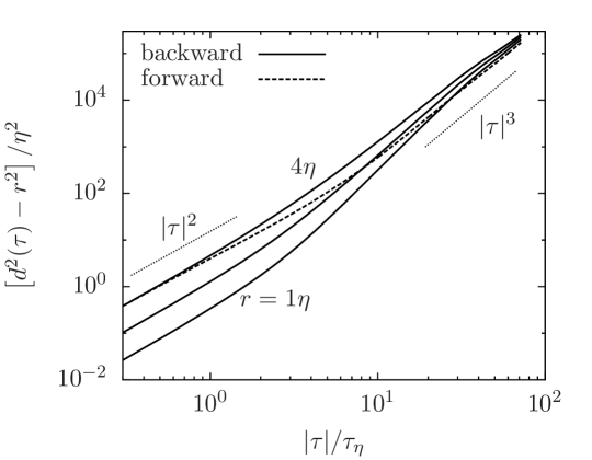
Figure 20.— Separation of tracer particle pairs in our simulated flow. The time lag and the particle separation are normalized to Kolmogorov time and length scales. Solid lines from top to bottom correspond to the backward separation of particle pairs with “initial” distance $r=1$, $2$ and $4\eta$, respectively. The dashed line plots the forward separation with $r=4\eta$. The initial time is set to 0, and $\tau$ is negative (positive) for the backward (forward) separation. The separation shows a ballistic phase and a Richardson behavior at small and large $|\tau|$, respectively.

The Richardson separation behavior (the $|\tau|^{3}$ scaling) is observed at large $|\tau|$ after the particle separation enters the inertial range of the flow. In the bottom solid curve for $r=1\eta$, a $|\tau|^{3}$ scaling exists in a very limited range. A rough estimate of the Richardson constant in that range gives $g\simeq 0.5$. Consistent with previous studies (e.g., Sawford et al. 2008), the time range that exhibits the Richardson scaling becomes broader as $r$ increases to $4\eta$. This allows a more accurate estimate of $g$, and we find $g\simeq 1.2$ for $r=4\eta$, consistent with the experimental results of Berg et al. (2006). Similar to Sawford et al. (2008), the measured $g$ has a dependence on $r$. If the inertial range of the flow is considerably broader and the Richardson behavior exists in a larger time range, the curves for different initial distances are expected to converge at sufficiently large time lags, with $g$ eventually approaching a universal value.

The dashed line in Fig. 20 plots the forward-in-time pair dispersion of tracer particles at $r=4\eta$. A comparison with the top solid line shows that the forward separation is slower than the backward separation. For $r=4\eta$, $g$ is estimated to be 0.5 in the forward separation, about twice smaller than the value (1.2) for the corresponding backward separation. This is consistent with the result of Berg et al. (2006). A physical explanation for the faster backward separation will be given in Appendix B. In our model for the relative velocity of inertial particles, it is the backward separation that is relevant, and the purpose of showing an example for the forward separation in Fig. 20 is to illustrate the difference between the forward and backward separations.

The Richardson constant, $g$, in the tracer-like phase of inertial particle separation may be different from tracers. However, it is reasonable to assume that $g$ for the backward separation of inertial particles lies in a similar range. Like tracers, the value of $g$ for inertial particles may also depend on the initial distance, $r$. In §6.1, we adjusted the value of $g$ in our model to obtain best fits to the simulation results for the rms relative velocity at different $r$.

Appendix B B: The PDFs of the Turbulent Velocity Field

In this Appendix, we analyze the probability distribution functions (PDF) of the flow velocity increments. We measure the PDFs, $P_{\rm u}(\Delta u_{\rm r},\ell)$ and $P_{\rm u}(\Delta u_{\rm t},\ell)$, of the longitudinal and transverse increments as a function of the length scale, $\ell$. Similar to the computation of the structure functions in §4.2, the PDF measurement also uses the velocity differences along the three directions of the simulation grid. The variances of $P_{\rm u}(\Delta u_{\rm r},\ell)$ and $P_{\rm u}(\Delta u_{\rm t},\ell)$ correspond to the longitudinal ($S_{\rm ll}(\ell)$) and transverse ($S_{\rm nn}(\ell)$) structure functions, which have been shown in Fig. 3 (see §4.2). Clearly, the PDFs are wider at larger scales. Also, $P_{\rm u}(\Delta u_{\rm t},\ell)$ is wider than $P_{\rm u}(\Delta u_{\rm r},\ell)$ because $S_{\rm nn}(\ell)\geq S_{\rm ll}(\ell)$ at all $\ell$ (see Fig. 3).

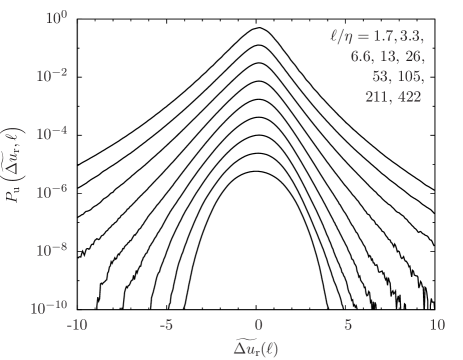
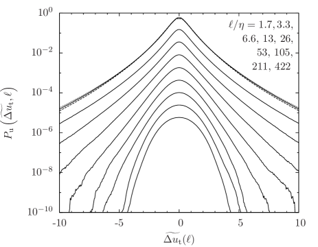
Figure 21.— The normalized PDFs of the flow velocity increment in the radial (left panel) and transverse (right panel) directions at different length scales, $\ell$. The normalized velocity increments are defined as $\widetilde{\Delta u_{\rm r}}(\ell)\equiv{\Delta u_{\rm r}}(\ell)/S_{\rm ll}^{1/2}(\ell)$ and $\widetilde{\Delta u_{\rm t}}(\ell)\equiv{\Delta u_{\rm t}}(\ell)/S_{\rm nn}^{1/2}(\ell)$. The top line in each panel plots the exact PDF at $\ell=1.7\eta$ (the cell size), and, for clarity, the PDF at each larger $\ell$ is shifted downward by a factor of 4. Except at the largest scales, the PDF, $P_{\rm u}(\widetilde{\Delta u_{\rm r}},\ell)$, of the radial increment has a negative skewness, whereas $P_{\rm u}(\widetilde{\Delta u_{\rm t}},\ell)$ for the transverse increment is symmetric at all scales. The PDF tails are highly non-Gaussian at small scales. With increasing $\ell$, the PDFs become less fat and finally approach Gaussian. In the right panel, the dashed and dotted lines for $\ell=1.7\eta$ are the normalized PDFs of the transverse increment conditioned on $\Delta u_{\rm r}<0$ and $\Delta u_{\rm r}>0$, respectively. One may change the normalization of $\ell$ to the integral scale, $L$, using $L=135\eta$.

To better see the PDF shape as a function of $\ell$, we normalized the PDFs at each scale to have unit variance. The radial and transverse velocity increments are normalized to their rms values, i.e., $\widetilde{\Delta u_{\rm r}}(\ell)\equiv{\Delta u_{\rm r}}(\ell)/S_{\rm ll}^{1/2}(\ell)$ and $\widetilde{\Delta u_{\rm t}}(\ell)\equiv{\Delta u_{\rm t}}(\ell)/S_{\rm nn}^{1/2}(\ell)$. The left panel of Fig. 21 shows the normalized PDF, $P_{\rm u}(\widetilde{\Delta u_{\rm r}},\ell)$, of the radial increment. Except at the largest scales, the PDF is negatively skewed. For inertial-range scales, this can be understood from Kolmogorov’s 4/5 law, $\langle\Delta u_{\rm r}(\ell)^{3}\rangle=-\frac{4}{5}\bar{\epsilon}\ell$, which indicates a negative skewness for the PDF of $\Delta u_{\rm r}$. The connection of the 3rd order moment of $\Delta u_{\rm r}$ to the energy dissipation rate suggests that the skewness originates from the dissipative nature of turbulence. The skewness of the PDF of $\Delta u_{\rm r}$ also provides an explanation for the faster backward separation found in Appendix A. The left and right tails of $P_{\rm u}(\widetilde{\Delta u_{\rm r}},\ell)$ correspond to tracer pairs receding from each other backward and forward in time, respectively. The broader left tail of the PDF thus suggests that the backward separation of tracer particles is faster than the forward case. Unlike $P_{\rm u}(\widetilde{\Delta u_{\rm r}},\ell)$, the PDF, $P_{\rm u}(\widetilde{\Delta u_{\rm t}},\ell)$, of the transverse increment in the right panel is symmetric at all $\ell$, as expected from statistical isotropy.

Both $P_{\rm u}(\widetilde{\Delta u_{\rm r}},\ell)$ and $P_{\rm u}(\widetilde{\Delta u_{\rm t}},\ell)$ are close to Gaussian at the largest scales, $\ell=211\eta$ (1/4 box size, or 1.6 times the integral scale, $L$) and $422\eta$ (1/2 box size, or $3.1L$), of the simulated flow. This is consistent with the Gaussian 1-point statistics in fully developed turbulence. At smaller $\ell$, the PDFs become non-Gaussian, and the tails keep getting fatter with decreasing $\ell$, a phenomenon known as intermittency in turbulence theory (Frisch 1995). As mentioned in the text, we use the word “fat” (or “thin”) specifically for the shape of the PDF, while “broad” (or “narrow”) refers to the extension or width of the PDF. The smallest scale, $1.7\eta$, in the figure corresponds to the size, $\Delta x$, of the computational cell. The shape of the normalized PDF is expected to remain unchanged once $\ell$ becomes smaller than $\sim\eta$. Physically, the viscosity acts to smooth the velocity field and makes it differentiable in the dissipation range, and thus the velocity increment at any scale $\ell\;\hbox to0.0pt{\lower 2.5pt\hbox{$\sim$}\hss}\raise 1.5pt\hbox{$<$}\;\eta$ is proportional to the local velocity gradient, whose PDF is fixed. In our simulation, the velocity field inside a computation cell is obtained by interpolation, and thus the PDF of the velocity difference below the cell size is controlled by the velocity gradient PDF at $\Delta x$. In §6.2, we showed that the trend of the PDF shape of the flow velocity difference with $\ell$ has interesting effects on the PDF of the relative velocity of inertial particles as a function of the particle inertia.

The tails of $P_{\rm u}(\widetilde{\Delta u_{\rm t}},\ell)$ for the transverse increment can be approximately described by stretched exponentials, $P_{\rm se}$ (see eq. (34) in §6.2). At largest scales, $P_{\rm u}(\widetilde{\Delta u_{\rm t}},\ell)$ are nearly Gaussian, and $\alpha=2$. With decreasing $\ell$, $\alpha$ decreases, corresponding to fatter tails. For example, the best-fit $\alpha$ for $P_{\rm u}(\widetilde{\Delta u_{\rm t}})$ at $\ell=26\eta$ is $\simeq 1$, and it further decreases to $\simeq 0.72$ at $\ell=1.7\eta$. Due to the asymmetry of the radial PDF, $P_{\rm u}(\widetilde{\Delta u_{\rm r}},\ell)$, one needs to obtain the fits separately for the left and right wings. Comparing the left wing of $P(\widetilde{\Delta u_{\rm r}},\ell)$ with $P_{\rm u}(\widetilde{\Delta u_{\rm t}},\ell)$, we see that their shape has a similar level of fatness at the same scale $\ell$. In fact, the best-fit $\alpha$ for the left tail of $P_{\rm u}(\widetilde{\Delta u_{\rm r}},\ell)$ is very close to that for $P_{\rm u}(\widetilde{\Delta u_{\rm t}},\ell)$. We also find that the best-fit values of $\alpha$ for the left and right tails of $P_{\rm u}(\widetilde{\Delta u_{\rm r}},\ell)$ are close, indicating that the two tails have a similar shape and differ only in the fluctuation amplitude.

To quantify the fluctuation amplitudes in the left and right wings of $P_{\rm u}(\Delta u_{\rm r},\ell)$, we define the variances in the two wings as $\langle\Delta u_{\rm r}^{2}\rangle_{-}=\int_{-\infty}^{0}\Delta u_{\rm r}^{2}P_{\rm u}(\Delta u_{\rm r},\ell)d\Delta u_{\rm r}/\int_{-\infty}^{0}P_{\rm u}(\Delta u_{\rm r},\ell)d\Delta u_{\rm r}$ and $\langle\Delta u_{\rm r}^{2}\rangle_{+}=\int_{0}^{\infty}\Delta u_{\rm r}^{2}P_{\rm u}(\Delta u_{\rm r},\ell)d\Delta u_{\rm r}/\int_{0}^{\infty}P_{\rm u}(\Delta u_{\rm r},\ell)d\Delta u_{\rm r}$. The definition of $\langle\Delta u_{\rm r}^{2}\rangle_{\mp}$ is similar to $\langle w_{\rm r}^{2}\rangle_{\mp}$ for the relative velocity of inertial particles (§6.1.3). We find that the ratio of $\langle\Delta u_{\rm r}^{2}\rangle_{-}$ to $\langle\Delta u_{\rm r}^{2}\rangle_{+}$ is $\simeq 1.47$ at $\ell=1.7\eta$. This ratio decreases with increasing $\ell$, and reaches unity at the largest scales. The variances of the left and right wings of $P_{\rm u}(\Delta u_{\rm r},\ell)$ was used in the discussion on the relative velocity of approaching and separating particle pairs in the $St\ll 1$ limit (see §6.1.3). We also considered the PDF of $\Delta u_{\rm t}$ conditioned on the sign of $\Delta u_{\rm r}$. We denote two conditional PDFs as $P_{\rm u}(\Delta u_{\rm t}|\Delta u_{\rm r}\lessgtr 0,\ell)$ and their variances as $\langle\Delta u_{\rm t}^{2}\rangle_{\mp}\equiv\int_{-\infty}^{\infty}\Delta u_{\rm t}^{2}P_{\rm u}(\Delta u_{\rm t}|\Delta u_{\rm r}\lessgtr 0,\ell)d\Delta u_{\rm t}$. At $\ell=1.7\eta$, $\langle\Delta u_{\rm t}^{2}\rangle_{-}$ is found to be larger than $\langle\Delta u_{\rm t}^{2}\rangle_{+}$ by 28%. In the right panel of Fig. 21, the dashed and dotted lines show the normalized conditional PDFs, $P_{\rm u}(\widetilde{\Delta u_{\rm t}}|\Delta u_{\rm r}<0,\ell)$ and $P_{\rm u}(\widetilde{\Delta u_{\rm t}}|\Delta u_{\rm r}>0,\ell)$, at $\ell=1.7\eta$. The conditional variances and PDFs of $\Delta u_{\rm t}$ are useful to understand the tangential relative velocity of approaching and separating particle pairs with $St\ll 1$ (§6.1.3 and 6.2.4).

References

- (1)
- (2) Abrahamson, J. 1975, Chem. Eng. Sci. 30, 1371
- (3) Ayala, O., Rosa, B. & Wang, L.-P. 2008, New J. Physics,10, 075016
- (4) Balkovsky, E., Falkovich, G., & Fouxon, A. 2001, Phys. Rev. Lett., 86, 2790
- (5) Bec, J., Biferale, L., Cencini, M., Lanotte, A. S., & Toschi, F. 2009, arXiv: 0905.1192v1 [physics.fly-dyn]
- (6) Bec, J., Biferale, L., Lanotte, A. S., Scagliarini, A., & Toschi, F. 2010, J. Fluid Mech., 645, 497
- (7) Berg, J., Luthi, B., Mann, J. & Ott, S. 2006, Phys. Rev. E., 74, 016304
- (8) Birnstiel, T., Ormel, C. W., & Dullemond, C. P. 2011, A&A, 525, 11
- (9) Blum, J. & Wurm, G. 2008, ARAA, 46, 21
- (10) Brandenburg, A. & Dobler, W. 2002, Computer Physics Communications, 147, 471
- (11) Chambers, J. E. 2010, Icarus, 208, 505
- (12) Chiang, E. 2008, ApJ, 675, 1549
- (13) Cuzzi, J. N. & Hogan R. C. 2003, Icarus,164, 127
- (14) Cuzzi, J. N., Hogan, R. C., & Bottke, W. F. 2010, Icarus, 208, 518
- (15) Cuzzi, J. N., Hogan, R. C., Paque, J. M., & Dobrovolskis, A. R. 2001, ApJ, 546, 496
- (16) Cuzzi, J. N., Hogan, R. C. & Shariff, K. 2008, ApJ, 687, 1432
- (17) de Jong J., Salazar, J. P. L. C., Woodward, S. H., Collins, L. R., & Meng, H. 2010, Int. J. Multiphase Flow, 36, 324
- (18) Dullemond, C. P. & Dominik, C. 2005, A&A, 434, 971
- (19) Falkovich, G., Fouxon, A., & Stepanov, M. G. 2002, Nature, 419, 151
- (20) Falkovich, G., & Pumir, A. 2004, Physics of Fluids, 16, L47
- (21) Falkovich, G. & Pumir, A. 2007, J. Atmos. Sci. 64, 4497
- (22) Freytag, B., Allard, F., Ludwig, H.-G., Homeier, D., & Steffen, M. 2010, A&A, 513, A19
- (23) Frisch, U. 1995, Turbulence. The Legacy of AN Kolmogorov (Cambridge University Press, Cambridge)
- (24) Garaud, P., Meru, F., Galvagni, M., & Olczak, C. 2013, ApJ, 764, 146
- (25) Girimaji, S. S. & Pope, S. B. 1990, J. Fluid. Mech., 220, 427
- (26) Goldreich, P., & Ward, W. R. 1973, ApJ, 183, 1051
- (27) Gustavsson, K. & Mehlig, B. 2011, Phys. Rev. E, 84, 045304(R)
- (28) Gustavsson, K., Mehlig, B., Wilkinson, M. & Uski, V. 2008, Phys. Rev. Lett., 101, 174503
- (29) Gustavsson, K., Meneguz, E., Reeks, M. & Mehlig, B. 2012, New J. Physics, 14, 115017
- (30) Guttler, C., Blum, J., Zsom, A., Ormel, C. W.,& Dullemond, C. P. 2010, A&A, 513, A56
- (31) Helling, Ch., Jardine, M. & Mokler, F. 2011, ApJ, 737, 38
- (32) Hockney, R. W., & Eastwood, J. W. 1981, Computer Simulation Using Particles, New York: McGraw-Hill
- (33) Hogan, R. C., & Cuzzi, J. N. 2001, Phys. Fluids, 13, 2938
- (34) Hubbard, A. 2012, MNRAS, 426, 784
- (35) Hubbard, A. 2013, MNRAS, 432, 1274
- (36) Ishihara, T., Gotoh, T. & Kaneda, Y. 2009, Annu. Rev. Fluid Mech., 41, 165
- (37) Johansen, A., Andersen, A. C., & Brandenburg, A. 2004, A&A, 417, 361
- (38) Johansen, A., Klahr, H., & Henning, Th. 2011, A&A, 529, A62
- (39) Johansen, A., Oishi, J. S., Low, M.-M. M., et al. 2007, Nature, 448, 1022
- (40) Johansen, A. & Youdin, A. N. 2007, ApJ, 662, 627
- (41) Johansen, A., Youdin, A., & Mac Low, M.-M. 2009, ApJ, 704, L75
- (42) Kolmorgorov, A. N. 1962, J. Fluid. Mech., 13, 82
- (43) Kruis, F. E. & Kusters, K. A. 1997, Chem. Eng. Comm., 158, 201
- (44) Lee, A. T., Chiang, E., Asay-Davis, X., & Barranco, J. 2010, ApJ, 725, 1938
- (45) Lundgren, T. S. 1981, J. Fluid Mech. 111, 27
- (46) Markiewicz, W. J., Mizuno, H. & Voelk, H. J. 1991, A&A, 242, 286
- (47) Maxey, M. R. 1987, J. Fluid Mech., 174, 441
- (48) Monin, A. S. & Yaglom, A. M. 1975, Statistical Fluid Mechanics: Mechanics of Turbulence, vol. 2. MIT press.
- (49) Ormel, C. W., & Cuzzi, J. N. 2007, A&A, 466, 413
- (50) Ormel, C. W., Paszun, D., Dominik, C., & Tielens, A. G. G. M. 2009, A&A, 502, 845
- (51) Padoan, P., Jimenez, R., Nordlund, A. & Boldyrev, S., 2004, Phys. Rev. Lett. 92, 191102
- (52) Pan, L. & Padoan, P. 2010, J. of Fluid Mech., 661, 73 (PP10)
- (53) Pan, L., Padoan, P.. Scalo, J., Kritsuk, A. G., & Norman, M. L. 2011, ApJ, 740, 21
- (54) Pan, L. & Scannapieco, E. 2011, Phys. Rev. E, 2011, 83, 045302(R)
- (55) Pinsky, M. B. & Khain, A. P. 1997, J. Aerosol Sci. 28, 1177
- (56) Pruppacher, H. R., & Klett, J. D. 1997, Microphysics of Clouds and Precipitation(Dordrecht: Kluwer)
- (57) Rossow, W.B., 1978, Icarus, 36, 1
- (58) Saffman, P. G. & Turner, J. S.1956 J. Fluid Mech., 1, 16
- (59) Sawford, B. L. 1991, Phys. Fluids, 3, 1577
- (60) Sawford, Yeung& Hackl]saw08 Sawford, B. L., Yeung, P. K. & Hackl, J. F. 2008, Phys. Fluids, 20, 065111
- (61) Shaw, R. A. 2003, Annu. Rev. Fluid Mech., 35, 183
- (62) Squires, K. D., & Eaton, J. K. 1991, Phys. Fluids, 3, 1169
- (63) Sundaram, S., & Collins, L. R. 1997, J. of Fluid Mech., 335, 75
- (64) Volk, H. J., Jones, F. C., Morfill, G. E.& Roeser, S. 1980, A&A, 85, 316–325
- (65) Wang, L.-P., Wexler, A. S., & Zhou, Y. 1998, Phys. Fluids, 10, 2467
- (66) Wang, L.-P., Wexler, A. S., & Zhou, Y. 2000, J. of Fluid Mech., 415, 117
- (67) Weidenschilling, S. J. 1980, Icarus, 44, 172
- (68) Wilkinson, M. & Mehlig, B. 2005, Europhys. Lett., 71, 186
- (69) Wilkinson, M. Mehlig, B., & Bezuglyy, V. 2006, Phys. Rev. Lett., 97, 048501
- (70) Williams, J. J. E. & Crane, R. I. 1983, Int. J. Multiphase Flow, 9, 421
- (71) Windmark, F., Birnstiel, T., Ormel, C. W., & Dullemond, C. P. 2012, A&A, 544, L16
- (72) Yeung, P. K., Pope, S. B. & Sawford, B. L. 2006, J. Turbulence, 7, 58
- (73) Youdin, A. N. 2011, ApJ, 742, 38
- (74) Yuu, S. 1984, AIChE J., 30, 802
- (75) Zaichik, L. I., & Alipchenkov, V. M. 2003, Phys. Fluids, 15, 1776
- (76) Zaichik, L. I. & Alipchenkov, V. M. 2009, New J. Phys., 11, 103018
- (77) Zaichik, L. I., Simonin, O. & Alipchenkov, V. M. 2003, Phys. Fluids, 15, 2995
- (78) Zaichik, L. I., Simonin, O. & Alipchenkov, V. M. 2006, Phys. Fluids,18, 035110
- (79) Zhou, Y., Wexler, A. S., & Wang, L.-P. 2001, J. Fluid Mech., 433, 77
- (80) Zsom, A., Ormel, C. W., Dullemond, C. P., & Henning, T. 2011, A&A, 534, A73
- (81) Zsom, A., Ormel, C. W., Güttler, C., Blum, J., & Dullemond, C. P. 2010, A&A, 513, A57
- (82)