Unitarity Saturation In P-P Scattering

Abstract

The properties of soft p-p scattering amplitudes at the TeV-scale are studied so as to identify the impact of s and t channel unitarity screenings on their behavior at exceedingly high energies and determine the rate at which they approach the bounds implied by unitarity saturation. I shall examine the relevant high energy soft cross section features, as well as, the corresponding behavior of the coupled phenomenological models aiming to reproduce this data.
My conclusion is that p-p black body saturation is not attained up to 100 TeV. More over, I do not expect that saturation will be attained at energies that can be investigated experimentally.

I INTRODUCTION

Following are 3 paradoxes, dating back to the ISR epoch, which are resolved by the introduction of unitarity screenings.

• Whereas non screened $\sigma_{tot}$ grows like $s^{\Delta}$, $\sigma_{el}$ grows faster, like $s^{2\Delta}$ (up to logarithmic corrections). With no screening, $\sigma_{el}$ will, eventually, be larger than $\sigma_{tot}$.

• Elastic and diffractive scatterings are seemingly similar. However, the energy dependence of the diffractive cross sections is significantly more moderate than that of $\sigma_{el}$.

• The elastic amplitude is central in impact parameter b-space, peaking at b=0. The diffractive amplitudes are peripheral peaking at large b, which gets larger with energy.

In the following I wish to explore the features of elastic scattering and inelastic diffractive scattering and their impact on our investigation of unitarity screenings. As we shall see, models confined only to elastic scattering are single dimension. Incorporating diffraction in our formalism implies a two dimension presentation of the unitarity equation. Recall, though, that enforcing unitarity is model dependent.
Added to our data analysis, is the output of two updated versions of the Pomeron (${I\!\!P}$) model. Regardless of their differences, GLM and KMR models provide compatible procedures to calculate both s and t channel screenings of elastic and diffractive scattering. The two models have a single partonic Pomeron. Its hardness depends on the ${I\!\!P}$ screenings(GLM), or the transverse momenta of its partons(KMR).
Current ${I\!\!P}$ models have a relatively large $\Delta_{{I\!\!P}}$ and exceedingly small (non zero) $\alpha_{{I\!\!P}}^{\prime}$, which seemingly disagree with the conventional features of the Regge Pomeron, in which the s dependence of a ${I\!\!P}$ exchange amplitude is determined by $\Delta_{{I\!\!P}}$ and the shrinkage of its forward t slope by $\alpha_{{I\!\!P}}^{\prime}$. In the ${I\!\!P}$ models, the traditional Regge features are restored by s and t unitarity screenings.
Both GLM and KMR utilize the approximation $\alpha_{{I\!\!P}}^{\prime}=0$. This assumption is critical for the input of a single Pomeron, and the summation of higher order ${I\!\!P}$ diagrams. It implies an upper validity bound of these models at 60-100 TeV.
Since I wish to assess unitarity saturation also above 100 TeV, I have included in the analysis also the Block-Halzen calculations of the total and inelastic cross sections in a single channel model based on a logarithmic parametrization. This model can be applied at arbitrary high energies. Recall that, single channel models are deficient since they neglect the diffractive channels.
This talk aims to assess the approach of p-p scattering amplitudes toward s and t unitarity saturation. The analysis I shall present is based on:

• General principles manifested by Froissart-Martin asymptotic bound of p-p total cross sections, introduced 50 years ago.

• TeV-scale p-p data analysis based on the output of the TEVATRON, LHC, and AUGER (in which p-p features are calculated from p-Air Cosmic Rays data).

• As we shall see, the TEVATRON(1.8)-LHC(7)-AUGER(57) data indicate that soft scattering amplitudes populate a small, slow growing, fraction of the available phase space confined by unitarity bounds.

• Phenomenological unitarity models substantiate the conclusions obtained from the available data analysis. Model predictions suggest that saturation is attained (if at all) at much higher energies well above experimental reach.

II S CHANNEL UNITARITY

The simplest s-channel unitarity bound on $a_{el}(s,b)$ is obtained from a diagonal re-scattering matrix, where repeated elastic re-scatterings secure s-channel unitarity:

$$2Ima_{el}(s,b)={\mid}a_{el}(s,b){\mid}^{2}+G^{in}(s,b).$$ (II.1)

Its general solution is

$$a_{el}(s,b)\, = \,i\left(1-e^{-\Omega(s,b)/2}\right),$$

$$G^{in}(s,b)\, = \,1\,-e^{-\Omega(s,b)}.$$ (II.2)

$\Omega$ is arbitrary. The output s-unitarity bound is $\mid a_{el}(s,b)\mid\leq 2$, leading to very large total and elastic LHC cross sections, which are not supported by the recent Totem data.

Figure 1: The effect of eikonal screening restoring s-unitarity. The schematic bound implied by analyticity/crossing is also shown.

In a Glauber type eikonal approximation, the input opacity $\Omega(s,b)$ is real. It equals to the imaginary part of the input Born term, a ${I\!\!P}$ exchange in our context. The output $a_{el}(s,b)$ is imaginary.
The consequent bound is $\mid a_{el}(s,b)\mid\leq 1,$ which is the black disc bound.
Analyticity and crossing symmetry are restored by the dispersion relation substitution

$$s^{\alpha_{{I\!\!P}}}\,\rightarrow\,s^{\alpha_{{I\!\!P}}}e^{-\frac{1}{2}i\pi\alpha_{{I\!\!P}}}.$$ (II.3)

In a single channel eikonal model, the screened cross sections are:

$$\sigma_{tot} = 2\displaystyle\int d^{2}b\left(1-e^{-\Omega(s,b)/2}\right),$$ (II.4)

$$\sigma_{el} = \displaystyle\int d^{2}b\left(1-e^{-\Omega(s,b)/2}\right)^{2},$$ (II.5)

$$\sigma_{inel} = \displaystyle\int d^{2}b\left(1-e^{-\Omega(s,b)}\right).$$ (II.6)

An illustration of the effects implied by unitarity screenings are shown in Fig.1. It shows the s-channel black bound of unity, and the bound implied by analyticity/crossing symmetry on the expanding b-amplitude.
Imposing these limits leads to the Froissart-Martin bound:

$$\sigma_{tot}\, \leq \,Cln^{2}(s/s_{0}),$$

$$s_{0} = 1GeV^{2},$$

$$C\, \propto \,1/2m^{2}_{\pi}\simeq 30mb.$$ (II.7)

C is far too large to be relevant in the analysis of TeV-scale data.
Coupled to Froissart-Martin is MacDowell-Martin bound:    $\frac{\sigma_{tot}}{B_{el}}\,\leq\,18\,\pi\,\frac{\sigma_{el}}{\sigma_{tot}}.$
Note that the Froissart limit controls the asymptotic behavior of the unitarity cross section bound, NOT the behavior of the elastic scattering cross section as such, which can have an arbitrary functional behavior as long as it is bellow saturation.
There have been recent suggestions by Azimov, Fagundes et al., and Achilli et al., to revise the normalization and/or the functional behavior of the bound. As it stands, these attempts are not relevant to our analysis.
In t-space, $\sigma_{tot}$ is proportional to a single point, $d\sigma_{el}/dt(t=0)$ (optical theorem).
As we saw, $\sigma_{tot}$ in b-space is obtained from a $b^{2}$ integration over $2(1-e^{-\frac{1}{2}\Omega(s,b)}).$
Saturation in b-space is, thus, a differential feature, attained initially at b=0 and then expands very slowly with energy. Consequently, a black core is a product of partial saturation, different from a complete saturation in which $a_{el}(s,b)$ is saturated at all b.
In a single channel model, $\sigma_{el}\leq\frac{1}{2}\sigma_{tot}$ and $\sigma_{inel}\geq\frac{1}{2}\sigma_{tot}.$
At saturation, regardless of the energy at which it is attained,

$$\sigma_{el}=\sigma_{inel}=\frac{1}{2}\sigma_{tot}.$$ (II.8)

Introducing diffraction, will significantly change the features of unitarity screenings. However, the saturation signatures remain valid.

III TEV-SCALE DATA

Following is p-p TeV-scale data relevant to the assessment of saturation:
CDF(1.8 TeV):

$$\sigma_{tot} = 80.03\pm 2.24mb,$$

$$\sigma_{el} = 19.70\pm 0.85mb,$$

$$B_{el} = 16.98\pm 0.25GeV^{-2}.$$

TOTEM(7 TeV):

$$\sigma_{tot} = 98.3\pm 0.2(stat)\pm 2.8(sys)mb,$$

$$\sigma_{el} = 24.8\pm 0.2(stat)\pm 1.2(sys)mb,$$

$$B_{el} = 20.1\pm 0.2(stat)\pm 0.3(sys)GeV^{-2}.$$

AUGER(57 TeV):

$$\sigma_{tot} = 133\pm 13(stat){\pm}^{17}_{20}(sys)\pm 16(Glauber)mb,$$

$$\sigma_{inel} = 92\pm 7(stat)\pm^{9}_{11}(sys)\pm 16(Glauber)mb.$$

Consequently:

$$\sigma_{inel}/\sigma_{tot}(CDF)\, = \,0.75,$$

$$\sigma_{inel}/\sigma_{tot}(TOTEM)\, = \,0.75,$$

$$\sigma_{inel}/\sigma_{tot}(AUGER)\, = \,0.69.$$

$$\sigma_{tot}/B_{el}(TOTEM) = 12.6<14.1.$$

The ratios above imply that saturation of the elastic p-p amplitude has NOT been attained up to 57 TeV. Note that the margin of AUGER errors is large. Consequently, saturation studies in the TeV-scale need the support of phenomenological models!

IV POMERON MODEL

Translating the concepts presented into a viable phenomenology requires a specification of $\Omega(s,b)$, for which Regge theory is a powerful tool. Pomeron (${I\!\!P}$) exchange is the leading term in the Regge hierarchy.
The growing total and elastic cross sections in the ISR-Tevatron range are well reproduced by the non screened single channel DL ${I\!\!P}$ model in which:

$$\alpha_{{I\!\!P}}(t) = 1+\Delta_{{I\!\!P}}+\alpha^{\prime}_{{I\!\!P}}t,$$

$$\Delta_{{I\!\!P}} = 0.08,$$

$$\alpha^{\prime}_{{I\!\!P}} = 0.25GeV^{-2}.$$ (IV.9)

$\Delta_{{I\!\!P}}$ determines the energy dependence, and $\alpha^{\prime}_{{I\!\!P}}$ the forward slopes.
Regardless of DL remarkable success at lower energies, they under estimate the LHC cross sections. This is traced to DL neglect of diffraction and unitarity screenings initiated by s and t dynamics. Updated Pomeron models analyze elastic and diffractive channels utilizing s and t unitarity screenings.

IV.1 Good-Walker Decomposition

Consider a system of two orthonormal states, a hadron $\Psi_{h}$ and a diffractive state $\Psi_{D}$. $\Psi_{D}$ replaces the continuous diffractive Fock states. Good-Walker (GW) noted that $\Psi_{h}$ and $\Psi_{D}$ do not diagonalize the 2x2 interaction matrix ${\bf T}$.
Let $\Psi_{1}$, $\Psi_{2}$ be eigen states of $\bf T.$

$$\Psi_{h}=\alpha\,\Psi_{1}+\beta\,\Psi_{2},$$

$$\Psi_{D}=-\beta\,\Psi_{1}+\alpha\,\Psi_{2},$$

$$\alpha^{2}+\beta^{2}=1,$$ (IV.10)

initiating 4 $A_{i,k}$ elastic GW amplitudes $(\psi_{i}+\psi_{k}\rightarrow\psi_{i}+\psi_{k}).$ i,k=1,2.
For initial $p({\bar{p}})-p$ we have $A_{1,2}=A_{2,1}$. I shall follow the GLM definition, in which the mass distribution associated with $\Psi_{D}$ is not defined.
The elastic, SD and DD amplitudes in a 2 channel GW model are:

$$a_{el}(s,b)=i\{\alpha^{4}A_{1,1}+2\alpha^{2}\beta^{2}A_{1,2}+\beta^{4}A_{2,2}\},$$ (IV.11)

$$a_{sd}(s,b)=i\alpha\beta\{-\alpha^{2}A_{1,1}+(\alpha^{2}-\beta^{2})A_{1,2}+\beta^{2}A_{2,2}\},$$ (IV.12)

$$a_{dd}(s,b)=i\alpha^{2}\beta^{2}\{A_{1,1}-2A_{1,2}+A_{2,2}\}.$$ (IV.13)

$$A_{i,k}(s,b)=\left(1-e^{\frac{1}{2}\Omega_{i,k}(s,b)}\right)\leq 1.$$ (IV.14)

GW mechanism changes the structure of s-unitarity below saturation.

• In the GW sector we obtain the Pumplin bound: $\sigma_{el}+\sigma_{diff}^{GW}\leq\frac{1}{2}\sigma_{tot}$.
  $\sigma_{diff}^{GW}$ is the sum of the GW soft diffractive cross sections.

• Below saturation, $\sigma_{el}\leq\frac{1}{2}\sigma_{tot}-\sigma_{diff}^{GW}$ and $\sigma_{inel}\geq\frac{1}{2}\sigma_{tot}+\sigma_{diff}^{GW}.$

• $a_{el}(s,b)=1,$ when and only when, $A_{1,1}(s,b)=A_{1,2}(s,b)=A_{2,2}(s,b)=1$.

• When $a_{el}(s,b)=1,$ all diffractive amplitudes at (s,b) vanish.

• As we shall see, there is a distinction between GW and non GW diffraction. Regardless, GW saturation signatures are valid also in the non GW sector.

• As we saw, the saturation signature, $\sigma_{el}=\sigma_{inel}=\frac{1}{2}\sigma_{tot},$ in a multi channel calculation is coupled to $\sigma_{diff}=0.$ Consequently, prior to saturation the diffractive cross sections stop growing and start to decrease with energy. This is a clear signature preceding saturation.

V CROSSED CHANNEL UNITARITY

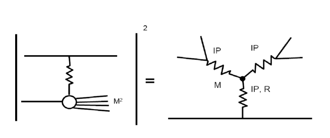
Figure 2: Mueller’s triple Regge diffractive diagram

Mueller(1971) applied 3 body unitarity to equate the cross section of $a\,+\,b\rightarrow M_{sd}^{2}\,+\,b$ to the triple Regge diagram $a\,+b\,+\bar{b}\rightarrow a\,+\,b\,+\,\bar{b}.$
The signature of this presentation is a triple vertex with a leading $3{I\!\!P}$ term. The 3${I\!\!P}$ approximation is valid, when $\frac{m_{p}^{2}}{M_{sd}^{2}}\,<<\,1$ and $\frac{M_{sd}^{2}}{s}\,<<\,1$.
The leading energy/mass dependences are

$$\frac{d\sigma^{3{I\!\!P}}}{dt\,dM_{sd}^{2}}\propto s^{2\Delta_{{I\!\!P}}}(\frac{1}{M_{sd}^{2}})^{1+\Delta_{{I\!\!P}}}.$$ (V.15)

Mueller’s 3${I\!\!P}$ approximation for non GW diffraction is the lowest order of t-channel multi ${I\!\!P}$ interactions, which induce compatibility with t-channel unitarity.
Recall that unitarity screening of GW (”low mass”) diffraction is carried out explicitly by eikonalization, while the screening of non GW (”high mass”) diffraction is carried out by the survival probability (to be discussed).

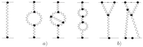
Figure 3: The Pomeron Green function.

Fig.3 shows the ${I\!\!P}$ Green function. Multi ${I\!\!P}$ interactions are summed differently in the various ${I\!\!P}$ models.
Note the analogy with QED renormalization:
a) Enhanced diagrams, present the renormalization of the propagator.
b) Semi enhanced diagrams, present the p${I\!\!P}$p vertex renormalization.

V.1 Survival Probability

The experimental signature of a ${I\!\!P}$ exchanged reaction is a large rapidity gap (LRG), devoid of hadrons in the $\eta-\phi$ lego plot, $\eta\,=\,-ln(tan\frac{\theta}{2})$.
$S^{2}$, the LRG survival probability, is a unitarity induced suppression factor of non GW diffraction, soft or hard:

$$S^{2}\,=\,{\sigma_{diff}^{screened}}/{\sigma_{diff}^{nonscreened}}.$$ (V.16)

It is the probability that the LRG signature will not be filled by debris (partons and/or hadrons) originating from either the s-channel re-scatterings of the spectator partons, or by the t-channel multi ${I\!\!P}$ interactions.
Denote the gap survival factor initiated by s-channel eikonalization $S_{eik}^{2}$, and the one initiated by t-channel multi ${I\!\!P}$ interactions, $S_{enh}^{2}.$
The eikonal re-scatterings of the incoming projectiles are summed over (i,k).
$S^{2}$ is obtained from a convolution of $S_{eik}^{2}$ and $S_{enh}^{2}.$ A simpler, approximation, is

$$S^{2}=S_{eik}^{2}\cdot S_{enh}^{2}.$$ (V.17)

VI THE PARTONIC POMERON

Current ${I\!\!P}$ models differ in details, but have in common a relatively large adjusted input $\Delta_{{I\!\!P}}$ and a very small $\alpha_{{I\!\!P}}^{\prime}$. The exceedingly small fitted $\alpha_{{I\!\!P}}^{\prime}$ implies a partonic description of the ${I\!\!P}$ which leads to a pQCD interpretation.
The microscopic sub structure of the ${I\!\!P}$ is obtained from Gribov’s partonic interpretation of Regge theory, in which the slope of the ${I\!\!P}$ trajectory is related to the mean transverse momentum of the partonic dipoles constructing the Pomeron and, consequently, the running QCD coupling:

$$\alpha_{{I\!\!P}}^{\prime}\, \propto \,1/<p_{t}>^{2},$$

$$\alpha_{S} \propto \pi/ln\left(<p_{t}^{2}>/\Lambda_{QCD}^{2}\right)<<1.$$ (VI.18)

We obtain a single ${I\!\!P}$ with hardness depending on external conditions.
This is a non trivial relation as the soft ${I\!\!P}$ is a simple moving pole in J-plane, while, the BFKL hard ${I\!\!P}$ is a branch cut approximated, though, as a simple pole with $\Delta_{{I\!\!P}}=0.2-0.3$, $\alpha_{{I\!\!P}}^{\prime}=0$. GLM and KMR models are rooted in Gribov’s partonic ${I\!\!P}$ theory with a hard pQCD ${I\!\!P}$ input. It is softened by unitarity screening (GLM), or the decrease of its partons’ transverse momentum (KMR).
Both models have a bound of validity, at 60(GLM) and 100(KMR) TeV, implied by their approximations. Consequently, as attractive as updated ${I\!\!P}$ models are, we can not utilize them above 100 TeV.
To this end, the only available models are single channel, most of which have a logarithmic parametrization input. The main deficiency of such models is that while they provide a good reproduction of the available total and elastic data, their predictions at higher energies are questionable since diffractive channels and t-channel screening are not included

VII IS SATURATION ATTAINABLE? (PHENOMENOLOGY)

VII.1 Total and Inelastic Cross Sections:

Table I compares $\sigma_{tot}$ and $\sigma_{inel}$ outputs of GLM, KMR and BH in the energy range of 7-100 TeV.
Note that, GLM predictions at 100 TeV are above the model validity bound.
As seen, the 3 models have compatible $\frac{\sigma_{inel}}{\sigma_{tot}}$ outputs in the TeV-scale which is significantly larger than 0.5.
The BH model can be applied at arbitrary high energies. The prediction of BH at the Planck-scale (1.22$\cdot 10^{16}TeV$) is, $\sigma_{inel}/\sigma_{tot}=1131mb/2067mb=0.55,$ which is below $a_{el}$ saturation. Recall, BH do not consider t-channel unitarity screening.

VII.2 $\Delta_{{I\!\!P}}^{eff}$ Dependence on Energy

	$7\,TeV$	$14\,TeV$	$57\,TeV$	$100\,TeV$
	GLM    KMR     BH	GLM    KMR      BH	GLM         BH	GLM   KMR      BH
$\sigma_{tot}\,$	98.6      97.4     95.4	109.0    107.5   107.3	130.0      134.8	139.0    138.8     147.1
$\sigma_{inel}\,$	74.0     73.6    69.0	81.1     80.3      76.3	95.2        92.9	101.5    100.7      100.0
$\frac{\sigma_{inel}}{\sigma_{tot}}$	0.75       0.76     0.72	0.74       0.75       0.71	0.73       0.70	0.73       0.73        0.68

Table 1: Total and elastic cross sections

TeV	1.8 $\rightarrow$   7.0	7.0 $\rightarrow$ 14.0	7.0 $\rightarrow$ 57.0	57.0 $\rightarrow$ 100.0	14.0 $\rightarrow$ 100.0
$\Delta_{eff}(GLM)$	0.081	0.072	0.066	0.060	0.062
$\Delta_{eff}(KMR)$	0.076	0.071			0.065
$\Delta_{eff}(BH)$	0.088	0.085	0.082	0.078	0.080

Table 2: $\Delta_{{I\!\!P}}^{eff}$ Dependence on Energy

	$7\,TeV$	$14\,TeV$	$57\,TeV$	$100\,TeV$
	GLM     KMR	GLM    KMR	GLM	GLM      KMR
$\sigma_{tot}\,$	98.6        97.4	109.0    107.5	130.0	134.0    138.8
$\sigma_{el}\,$	24.6       23.8	27.9      27.2	34.8	37.5       38.1
$\sigma^{GW}_{sd}\,$	10.7           7.3	11.5          8.1	13.0	13.6        10.4
$\sigma_{sd}\,$	14.88	17.31	21.68
$\sigma^{GW}_{dd}\,$	6.21          0.9	6.79         1.1	7.95	8.39        1.6
$\sigma_{dd}\,$	7.45	8.38	18.14
$\frac{\sigma_{el}+\sigma_{diff}^{GW}}{\sigma_{tot}}\,$	0.42        0.33	0.42      0.34	0.43	0.43          0.36

Table 3: Diffractive cross sections

$\Delta_{{I\!\!P}}^{eff}$ serves as a simple measure of the rate of cross section growth estimated as $s^{\Delta_{{I\!\!P}}^{eff}}.$ When compared with the adjusted input $\Delta_{{I\!\!P}}$, we can assess the strength of the applied screening.
The screenings of $\sigma_{tot},\sigma_{el},\sigma_{sd}$, $\sigma_{dd}$ and $M_{diff}^{2}$ are not identical. Hence, their $\Delta_{{I\!\!P}}^{eff}$ values are different. The cleanest determination of $\Delta_{{I\!\!P}}^{eff}$ is from the energy dependence of $\sigma_{tot}$. All other options require also a determination of $\alpha_{{I\!\!P}}^{\prime}.$
Table II compares $\Delta_{{I\!\!P}}^{eff}$ values obtained by GLM, KMR and BH. The continuous reduction of $\Delta_{{I\!\!P}}^{eff}$ is a consequence of s and t screenings.

VII.3 Diffractive Cross Sections

GLM and KMR total, elastic and diffractive cross sections are presented in Table III. KMR confine their predictions to the GW sector.
GLM GW $\sigma_{sd}$ and $\sigma_{dd}$ are larger than KMR. Their $\sigma_{tot}$ and $\sigma_{el}$ are compatible.
In both models, the GW components are compatible with the Pumplin bound.
The persistent growth of the diffractive cross sections indicates that saturation will be attained (if at all) well above the TeV-scale.
Analysis of diffraction, is hindered by different choices of signatures and bounds!

VII.4 MacDowell-Martin Bound

MacDowell-Martin Bound is

$$\frac{\sigma_{tot}}{B_{el}}\leq 18\pi\frac{\sigma_{el}}{\sigma_{tot}}.$$

GLM and KMR ratios and bounds are:

$$7~{}TeV:~{}~{}\frac{\sigma_{tot}}{B_{el}} = 12.5<14.1(GLM),$$

$$\frac{\sigma_{tot}}{B_{el}} = 12.3<13.8(KMR).$$

$$14~{}TeV:~{}~{}\frac{\sigma_{tot}}{B_{el}} = 13.0<14.5(GLM),$$

$$\frac{\sigma_{tot}}{B_{el}} = 12.8<14.3(KMR).$$

$$100~{}TeV:~{}~{}\frac{\sigma_{tot}}{B_{el}} = 13.8<15.3(GLM),$$

$$\frac{\sigma_{tot}}{B_{el}} = 13.8<15.5(KMR).$$

As seen, the ratios above are compatible with a non saturated $a_{el}(s,b)$ at the available energies.

VIII CONCLUSION

The analysis presented re-enforced the critical roll played by s and t channel unitarity screenings in hadron-hadron high energy interactions. This presentation centered on p-p collisions at the TeV-scale with special attention invested on an assessment of unitarity saturation. Since the formalism of unitarity screenings is model dependent we have to be careful in the definitions of signatures indicating the onsetting of saturation.

• A clear, model independent, saturation signature is

  $$\frac{\sigma_{el}}{\sigma_{tot}}\,=\,\frac{\sigma_{inel}}{\sigma_{tot}}\,=\,\frac{1}{2}.$$ (VIII.19)

  Checking the experimental available cross section data, leads to a definite conclusion that unitarity saturation in p-p scattering is NOT attained at the available energies. Checking the rate at which $\frac{\sigma_{inel}}{\sigma_{tot}}$ grows with energy, it is reasonable to conclude that saturation will not be attained at the TeV-scale and possibly (BH) up to the Planck-scale.

• Quite a few models confine their analysis exclusively to the p-p elastic channel. In my opinion, there is no way to bypass the coupling between the elastic and diffractive channels.

• Since diffraction cross sections vanish when unitarity saturation is attained, we can consider that a change in the energy dependence of the diffractive cross section from a very moderate increase with energy to a decrease toward zero is an early signature that p-p scattering is approaching saturation. Since such a behavior has not been observed or predicted, I presume that saturation will not be attained at energies that can be experimentally investigated.