Matrix Compression using the Nyström Method

Abstract

The Nyström method is routinely used for out-of-sample extension of kernel matrices. We describe how this method can be applied to find the singular value decomposition (SVD) of general matrices and the eigenvalue decomposition (EVD) of square matrices. We take as an input a matrix $M\in\mathbb{R}^{m\times n}$, a user defined integer $s\leq min(m,n)$ and $A_{M}\in\mathbb{R}^{s\times s}$, a matrix sampled from the columns and rows of $M$. These are used to construct an approximate rank-$s$ SVD of $M$ in $O\left(s^{2}\left(m+n\right)\right)$ operations. If $M$ is square, the rank-$s$ EVD can be similarly constructed in $O\left(s^{2}n\right)$ operations. Thus, the matrix $A_{M}$ is a compressed version of $M$. We discuss the choice of $A_{M}$ and propose an algorithm that selects a good initial sample for a pivoted version of $M$. The proposed algorithm performs well for general matrices and kernel matrices whose spectra exhibit fast decay.

Keywords: {Compression, SVD, EVD, Nyström, out-of-sample extension}

1 Introduction

Low rank approximation of linear operators is an important problem in the areas of scientific computing and statistical analysis. Approximation reduces storage requirements for large datasets and improves the runtime complexity of algorithms operating on the matrix. When the matrix contains affinities between elements, low rank approximation can be used to reduce the dimension of the original problem ([28, 12, 23]) and to eliminate statistical noise ([22]).

Our approach involves the choice of a small sub-sample from the matrix, followed by the application of the Nyström method for out-of-sample extension. The Nyström method ([2]), which originates from the field of integral equations, is a way of discretizing an integral equation using a simple quadrature rule. When given an eigenfunction problem of the form

$$\lambda f(x)=\int^{b}_{a}{M\left(x,y\right)f\left(y\right)dy},$$

the Nyström method employs a set of $s$ sample points $y_{1},\dots,y_{s}$ that approximate $f(x)$ as

$$\lambda\tilde{f}\left(x\right)\triangleq\frac{b-a}{s}\sum^{s}_{j=1}{M\left(x,y_{j}\right)f\left(y_{j}\right)}.$$

In recent years, the Nyström method has gained widespread use in the field of spectral clustering. It was first popularized by [32] for sparsifying kernel matrices by approximating their entries. The matrix completion approach of [17] also enables the approximation of eigenvectors. It was now possible to use the Nyström method in order to speed up algorithms that require the spectrum of a kernel matrix. Over time, Nyström based out-of-sample extensions have been developed for a wide range of spectral methods, including Normalized-Cut ([18, 5]), Geometric Harmonics ([11]) and others ([6]).

Other noteworthy methods for speeding up kernel based algorithms, which are not applicable to the proposed setting of this paper, are based on sampling [1], convex optimization [9] and integral equations. ACA [3, 4] is an important example in the latter category. ACA can be regarded as an efficient replacement of the SVD which is tailored to asymptotically smooth kernels. The kernel function itself is not required. ACA uses only few of the original entries for the approximation of the whole matrix and it was shown to have exponential convergence when used as part of the Nyström method.

In this paper, we present two extensions of the matrix completion approach of [17]. These allow us to form the SVD and EVD of a general matrix through the application of the Nyström method on a previously chosen sample.

In addition, we present a novel algorithm for selecting the initial sample to be used with the Nyström method. Our algorithm is applicable to general matrices whereas previous methods focused on kernel matrices. The algorithm uses a pre-existing low-rank decomposition of the input matrix. We show that our sample choice reduces the Nyström approximation error.

The paper is organized as follows: Section 2 describes the basic Nyström matrix form and the methods of [17] for finding the EVD of a Nyström approximated symmetric matrix. Section 3 outlines a Nyström-like method for out-of-sample extension of general matrices, starting with the SVD of a sample matrix. In section 4 we describe procedures that explicitly generate the canonical SVD and EVD forms for general matrices. Section 5 introduces the problem of sample choice and presents results that bound the accuracy of the algorithm in section 6. Section 6 presents our sample selection algorithm and analyzes its complexity. Experimental results on general and kernel matrices are presented in section 7.

2 Preliminaries

2.1 Square Nyström Matrix Form

Let $M\in{\mathbb{R}}^{n\times n}$ be a square matrix. We assume that the $M$ can be decomposed as

$$M=\left[\begin{array}[]{cc}A_{M}&B_{M}\\ F_{M}&C_{M}\end{array}\right]$$ (1)

where $A_{M}\in{\mathbb{R}}^{s\times s},B_{M}\in{\mathbb{R}}^{s\times\left(n-s\right)},F_{M}\in{\mathbb{R}}^{\left(n-s\right)\times s}$ and $C_{M}\in{\mathbb{R}}^{\left(n-s\right)\times\left(n-s\right)}$. The matrix $A_{M}$ is designated to be our sample matrix. The size of our sample is $s$, which is the size of $A_{M}$.

Let $U\Lambda U^{-1}$ be the eigen-decomposition of $A_{M}$, where $U\in{\mathbb{R}}^{s\times s}$ is the eigenvectors matrix and $\Lambda\in{\mathbb{R}}^{s\times s}$ is the eigenvalues matrix. Let $u^{i}\in{\mathbb{R}}^{s}$ be the column eigenvector belonging to eigenvalue $\lambda_{i}$. We aim to extend the column eigenvector (the discrete form of an eigenfunction) to the rest of $M$. Let $\hat{u}^{i}=\left[\begin{array}[]{cc}u^{i}&\tilde{u}^{i}\end{array}\right]^{T}\in{\mathbb{R}}^{n}$ be the extended eigenvector, where $\tilde{u}^{i}\in{\mathbb{R}}^{n-s}$ is the extended part. By applying the Nyström method to $u^{i}$, we get the following form for the $k^{th}$ coordinate in $\hat{u}^{i}$:

$$\lambda_{i}\hat{u}^{i}_{k}\simeq\frac{b-a}{s}\sum^{s}_{j=1}{M_{kj}\cdot u^{i}_{j}}.$$ (2)

By setting $\left[a,b\right]=[0,1]$ and presenting Eq. (2) in matrix product form we obtain

$$\lambda_{i}\tilde{u}^{i}=\frac{1}{s}F_{M}\cdot u^{i}.$$ (3)

This can be done for all the eigenvalues $\{\lambda_{i}\}_{i=1}^{s}$ of $A_{M}$. Denote $\tilde{U}=\left[\begin{array}[]{ccc}\tilde{u}^{1}&\dots&\tilde{u}^{s}\end{array}\right]\in{\mathbb{R}}^{(n-s)\times s}$. By placing all expressions of the form Eq. (3) side by side we have $\tilde{U}\Lambda=F_{M}U$. Assuming the matrix $A_{M}$ has non-zero eigenvalues (we return to this assumption in section 5.4), we obtain:

$$\tilde{U}=F_{M}U{\Lambda}^{-1}.$$ (4)

Analogically, we can derive a matrix representation for extending the left eigenvectors of $M$, denoted as $\tilde{V}\in{\mathbb{R}}^{s\times n-s}$:

$$\tilde{V}={\Lambda}^{-1}U^{-1}B_{M}.$$ (5)

Combining Eqs. (4) and (5) with the eigenvectors of $A_{M}$ yields the full left and right approximated eigenvectors:

$$\hat{U}=\left[\begin{array}[]{c}U\\ F_{M}U{\Lambda}^{-1}\end{array}\right],\ \ \hat{V}=\left[\begin{array}[]{cc}U^{-1}&{\Lambda}^{-1}U^{-1}B_{M}\end{array}\right].$$ (6)

The explicit “Nyström” representation of $\hat{M}$ becomes:

$$\begin{array}[]{c}\hat{M}=\hat{U}\Lambda\hat{V}=\left[\begin{array}[]{c}U\\ F_{M}U{\Lambda}^{-1}\end{array}\right]\Lambda\left[\begin{array}[]{cc}U^{-1}&{\Lambda}^{-1}U^{-1}B_{M}\end{array}\right]=\left[\begin{array}[]{cc}A_{M}&B_{M}\\ F_{M}&F_{M}A^{+}_{M}B_{M}\end{array}\right]=\\ \left[\begin{array}[]{c}A_{M}\\ F_{M}\end{array}\right]A^{+}_{M}\left[\begin{array}[]{cc}A_{M}&B_{M}\end{array}\right]\end{array}$$ (7)

where $A^{+}_{M}$ denotes the pseudo-inverse of $A_{M}$.

Equation (7) shows that the Nyström extension does not modify $A_{M},B_{M}$ and $F_{M}$, and that it approximates $C_{M}$ by $F_{M}A^{+}_{M}B_{M}$.

2.2 Decomposition of Symmetric Matrices

The algorithm given in [17] is a commonly used method for SVD approximation of symmetric matrices. For a given matrix, it computes the SVD of its Nyström approximated form. The SVD and EVD of a symmetric matrix coincide up to the signs of the singular (eigen-) values. Therefore the SVD can approximate both simultaneously. We describe the method of [17] in section 2.2.2.

2.2.1 Symmetric Nyström Matrix Form

When $M$ is symmetric, the matrix $M$ has the decomposition

$$M=\left[\begin{array}[]{cc}A_{M}&B_{M}\\ B^{T}_{M}&C_{M}\end{array}\right]$$ (8)

where $A_{M}\in{\mathbb{R}}^{s\times s},B_{M}\in{\mathbb{R}}^{s\times\left(n-s\right)}$ and $C_{M}\in{\mathbb{R}}^{(n-s)\times(n-s)}$. We replace $F_{M}$ in Eq. (1) with $B_{M}^{T}$.

By using reasoning similar to section 2.1, we can express the right and left approximated eigenvectors as:

$$\hat{U}=\left[\begin{array}[]{c}U\\ B^{T}_{M}U{\Lambda}^{-1}\end{array}\right],\ \ \hat{V}=\left[\begin{array}[]{cc}U^{-1}&{\Lambda}^{-1}U^{-1}B_{M}\end{array}\right].$$ (9)

The explicit “Nyström” representation of $\hat{M}$ becomes:

$$\begin{array}[]{c}\hat{M}=\hat{U}\Lambda\hat{V}=\left[\begin{array}[]{c}U\\ B^{T}_{M}U{\Lambda}^{-1}\end{array}\right]\Lambda\left[\begin{array}[]{cc}U^{-1}&{\Lambda}^{-1}U^{-1}B_{M}\end{array}\right]=\left[\begin{array}[]{cc}A_{M}&B_{M}\\ B^{T}_{M}&B_{M}^{T}A^{+}_{M}B_{M}\end{array}\right]=\\ \left[\begin{array}[]{c}A_{M}\\ B^{T}_{M}\end{array}\right]A^{+}_{M}\left[\begin{array}[]{cc}A_{M}&B_{M}\end{array}\right].\end{array}$$ (10)

2.2.2 Construction of SVD for Symmetric $\hat{\mathbf{M}}$

Our goal is to find the $s$ leading eigenvalues and eigenvectors of $\hat{M}$ without explicitly forming the entire matrix.

We begin with the decomposition of $M$ as in Eq. (8). The approximation technique in [17] uses the standard Nyström method in Eq. (9) to obtain $\hat{U}$. Then, the algorithm forms the matrix $Z=\hat{U}{\Lambda}^{1/2}$ such that $\hat{M}=ZZ^{T}=\hat{U}\Lambda{\hat{U}}^{T}$. The symmetric $s\times s$ matrix $Z^{T}Z$ is diagonalized as $F\Sigma F^{T}$. The eigenvectors of $\hat{M}$ are given by $U_{o}=ZF{\Sigma}^{-1/2}$ and the eigenvalues are given by $\Sigma$. To qualify for use in the SVD, $U_{o}$ and $\Sigma$ must meet the following requirements:

1. The columns of $U_{o}$ must be orthogonal. Namely, $U^{T}_{o}U_{o}=I$.

2. The SVD form of $U_{o}$ and $\Sigma$ must form $\hat{M}$. Formally, $\hat{M}=U_{o}\Sigma U^{T}_{o}$.

The following identities can be readily verified using our expressions for $U_{o}$ and $\Sigma$:

1. Bi-orthogonality: $U^{T}_{o}U_{o}={\Sigma}^{-1/2}F^{T}Z^{T}ZF{\Sigma}^{{\rm-}{\rm 1/2}}={\Sigma}^{{\rm-}{\rm 1/2}}F^{T}\left(F\Sigma F^{T}\right)F{\Sigma}^{{\rm-}{\rm 1/2}}=I;$

2. SVD form: $U_{o}\Sigma U^{T}_{o}=ZF{\Sigma}^{{\rm-}{\rm 1/2}}\cdot\Sigma\cdot{\Sigma}^{{\rm-}{\rm 1/2}}F^{T}Z^{T}=ZZ^{T}=\hat{M}.$

The computational complexity of the algorithm is $O\left(s^{2}n\right)$, where $s$ is the sample size and $n$ is the number of rows and columns of $M$. The bottleneck is in the computation of the matrix product $Z^{T}Z$.

2.2.3 A Single-Step Solution for the SVD of $\hat{\mathbf{M}}$

The “one-shot” solution in [17] assumes that $A_{M}$ has a square root matrix $A^{1/2}_{M}$. This assumption is true if the matrix is positive definite. Otherwise, it imposes some limitations on $A_{M}$. These will be discussed in section 4.3.

Let $A^{-1/2}_{M}$ be the pseudo-inverse of the square root matrix of $A_{M}$. Denote $G^{T}=A^{-1/2}_{M}\left[\begin{array}[]{cc}A_{M}&B_{M}\end{array}\right]$. From this definition we have $\hat{M}=GG^{T}$. The matrix $S\in{\mathbb{R}}^{s\times s}$ was defined in [17], where $S=G^{T}G=A_{M}+A^{-1/2}_{M}B_{M}B^{T}_{M}A^{-1/2}_{M}$. $S$ is fully decomposed as $U_{S}{\Lambda}_{S}U^{T}_{S}$. The orthogonal eigenvectors of $\hat{M}$ are formed as $U_{o}=GU_{S}{\Lambda}^{-1/2}_{S}$ and the eigenvalues are given in ${\Lambda}_{S}$.

The following required identities, as in section 2.2.2, can again be verified as follows:

1. Bi-orthogonality:
   $U^{T}_{o}U_{o}={\Lambda}^{-1/2}_{S}U^{T}_{S}G^{T}GU_{S}{\Lambda}^{-1/2}_{S}={\Lambda}^{-1/2}_{S}U^{T}_{S}SU_{S}{\Lambda}^{-1/2}_{S}={\Lambda}^{-1/2}_{S}U^{T}_{S}\cdot U_{S}{\Lambda}_{S}U^{T}_{S}\cdot U_{S}{\Lambda}^{-1/2}_{S}=I.$

2. SVD form: $U_{o}{\Lambda}_{S}U^{T}_{o}=GU_{S}{\Lambda}^{-1/2}_{S}\cdot{\Lambda}_{S}\cdot{\Lambda}^{-1/2}_{S}U^{T}_{S}G^{T}=GG^{T}=\hat{M}.$

The computational complexity remains the same (the bottleneck of the algorithm is the formation of $B_{M}B^{T}_{M}$). However this version is numerically more accurate. According to [17], the extra calculations in the general method of solution lead to an increase in the loss of significant digits.

3 Nyström-like SVD approximation

The SVD of a matrix can also be approximated via the basic quadrature technique of the Nyström method. In this case, we do not require an eigen-decomposition. Therefore, $M$ does not necessarily have to be square. Let $M\in{\mathbb{R}}^{m\times n}$ be a matrix with the decomposition given in Eq. (1). We begin with the SVD form $A_{M}=U\Lambda H$ where $U,H\in{\mathbb{R}}^{s\times s}$ are unitary matrices and ${\Lambda}\in{\mathbb{R}}^{s\times s}$ is diagonal. We assume that zero is not a singular value of $A_{M}$. Accordingly, $U$ can be formulated as:

$$U=A_{M}H{\Lambda}^{-1}.$$ (11)

Let $u^{i},h^{i}\in{\mathbb{R}}^{s}$ be the $i^{th}$ columns in $U$ and $H$, respectively. Let $u^{i}=\{u^{i}_{l}\}_{l=1}^{s}$ be the partition of $u^{i}$ into elements. By using Eq. (11), each element $u^{i}_{l}$ can be presented as the sum $u^{i}_{l}=\frac{1}{\lambda_{i}}\sum_{j=1}^{n}{M_{lj}\cdot h^{i}_{j}}$.

We can use the entries of $F_{M}$ as interpolation weights for extending the singular vector $u^{i}$ to the $k^{th}$ row of $M$, where $s+1\leq k\leq n$. Let $\tilde{u}^{i}=\{\tilde{u}^{i}_{k-s}\}_{k=s+1}^{n}\in{\mathbb{R}}^{n-s}$ be a column vector that contains all the approximated entries. Each element $\tilde{u}^{i}_{k-s}$ will be calculated as $\tilde{u}^{i}_{k-s}=\frac{1}{\lambda_{i}}\sum_{j=1}^{n}{M_{kj}\cdot h^{i}_{j}}$. Therefore, the matrix form of $\tilde{u}^{i}$ becomes $\tilde{u}^{i}=\frac{1}{\lambda_{i}}F_{M}\cdot h^{i}$.

Putting together all the $\tilde{u}^{i}$’s as $\tilde{U}=\left[\begin{array}[]{cccc}\tilde{u}^{1}&\tilde{u}^{2}&\dots&\tilde{u}^{s}\end{array}\right]\in{\mathbb{R}}^{n-s\times s}$, we get $\tilde{U}=F_{M}H{\Lambda}^{-1}$.

The basic SVD equation of $A_{M}$ can also be written as $H=A_{M}^{T}U\Lambda^{-1}$. We approximate the right singular vectors of the out-of-sample columns by employing a symmetric argument. We obtain $\tilde{H}=B^{T}_{M}U{\Lambda}^{-1}$.

The full approximations of the left and right singular vectors of $\hat{M}$, denoted by $\hat{U}$ and $\hat{H}$, respectively, are

$$\hat{U}=\left[\begin{array}[]{c}U\\ F_{M}H{\Lambda}^{-1}\end{array}\right],\ \ \hat{H}=\left[\begin{array}[]{c}H\\ B^{T}_{M}U{\Lambda}^{-1}\end{array}\right].$$ (12)

The explicit “Nyström” form of $\hat{M}$ becomes

$$\begin{array}[]{c}\hat{M}=\hat{U}\Lambda{\hat{H}}^{T}=\left[\begin{array}[]{c}U\\ F_{M}H{\Lambda}^{-1}\end{array}\right]\Lambda\left[\begin{array}[]{cc}H^{T}&{\Lambda}^{-1}U^{T}B_{M}\end{array}\right]=\left[\begin{array}[]{cc}A_{M}&B_{M}\\ F_{M}&F_{M}A^{+}_{M}B_{M}\end{array}\right]=\\ \left[\begin{array}[]{c}A_{M}\\ F_{M}\end{array}\right]A^{+}_{M}\left[\begin{array}[]{cc}A_{M}&B_{M}\end{array}\right]\end{array}$$ (13)

where $A^{+}_{M}$ denotes the pseudo-inverse of $A_{M}$. $\hat{M}$ does not modify $A_{M},B_{M}$ and $F_{M}$ but approximates $C_{M}$ by $F_{M}A_{M}^{+}B_{M}$. Note that the Nyström matrix form of the SVD is similar to Eq. (7), which is the Nyström form of the EVD matrix.

4 Decomposition of General Matrices

We will refer to a decomposition of $M$ given in Eq. (1) with the corresponding decomposition into $A_{M},B_{M},F_{M}$ and $C_{M}$. $\hat{M}$ denotes the approximated Nyström matrix.

This section presents procedures for explicit orthogonalization of the singular-vectors and eigenvectors of $\hat{M}$. Starting with $\hat{M}$ in the form of Eqs. (7) and (13), we find its canonical SVD and EVD form, respectively. Constructing these representations takes time and space that are linear in the dimensions of $M$.

4.1 Construction of EVD for $\hat{\textbf{M}}$

Let $M$ be a square matrix. We will approximate the eigenvalue decomposition of $\hat{M}$ without explicitly forming $\hat{M}$.

We begin with a matrix $M$ that is partitioned as in Eq. (1). By explicitly employing the Nyström method, we construct $\hat{U}$ and $\hat{V}$ as defined in Eq. (6). Then, we proceed by defining the matrices $G_{U}=\hat{U}{\Lambda}^{1/2}$ and $G_{V}={\Lambda}^{1/2}\hat{V}$. We directly compute the EVD of $G_{V}G_{U}$ as $F\Sigma F^{-1}$. The eigenvalues of $\hat{M}$ are given by $\Sigma$ and the right and left eigenvectors are $U_{o}=G_{U}F{\Sigma}^{-1/2}$ and $V_{o}={\Sigma}^{-1/2}F^{-1}G_{V}$, respectively.

The left and right eigenvectors are mutually orthogonal since

$$V_{o}U_{o}={\Sigma}^{-1/2}F^{-1}G_{V}\cdot G_{U}F{\Sigma}^{-1/2}={\Sigma}^{-1/2}F^{-1}\cdot F\Sigma F^{-1}\cdot F{\Sigma}^{-1/2}=I.$$

The EVD form of $U_{o},V_{o}$ and $\Sigma$ gives $\hat{M}$, as we see from

$$U_{o}\Sigma V_{o}=G_{U}F{\Sigma}^{-1/2}\cdot\Sigma\cdot{\Sigma}^{-1/2}F^{-1}G_{V}=G_{U}G_{V}=\hat{U}{\Lambda}^{1/2}\cdot{\Lambda}^{1/2}\hat{V}=\hat{M}.$$

These two properties qualify $U_{o}\Sigma V_{o}$ as the EVD of $\hat{M}$.

When $M$ is symmetric, the matrix $G_{V}$ is simply $G^{T}_{U}$. By using the terminology in section 2.2.2, we denote $G_{V}=Z$ and the matrix $G_{V}G_{U}$ is transformed into $ZZ^{T}$. From here on the method of solution in section 2.2.2 coincides with the current section. Hence, this form of EVD approximation generalizes the symmetric case.

The computational complexity is $O(s^{2}n)$, where $s$ is the sample size (the size of $A_{M}$) and $n$ is the size of $M$. The computational bottleneck is in the formation of $G_{V}G_{U}$.

4.1.1 A Single-Step Solution for the EVD for $\hat{\mathbf{M}}$

This solution method assumes that $A_{M}$ has a square root matrix $A^{1/2}_{M}$. From this assumption, we can modify the algorithm in section 4.1 to construct the EVD of $\hat{M}$ with fewer steps.

We define the matrices $G_{U}$ and $G_{V}$ to be

$$G_{U}=\left[\begin{array}[]{c}A_{M}\\ F_{M}\end{array}\right]A^{-1/2}_{M},\ \ \ G_{V}=A^{-1/2}_{M}\left[\begin{array}[]{cc}A_{M}&B_{M}\end{array}\right].$$

We proceed to explicitly compute the eigen-decomposition of $G_{V}G_{U}\in{\mathbb{R}}^{s\times s}$ as $G_{V}G_{U}=F\Sigma F^{-1}$. The eigenvalues of $\hat{M}$ are given by $\Sigma$ and the right and left eigenvectors of $\hat{M}$ are formed by $U_{o}=G_{U}F{\Sigma}^{-1/2}$ and $V_{o}={\Sigma}^{-1/2}F^{-1}G_{V}$, respectively. Again, we can verify the eigenvectors are mutually orthogonal:

$$V_{o}U_{o}={\Sigma}^{-1/2}F^{-1}G_{V}\cdot G_{U}F{\Sigma}^{-1/2}={\Sigma}^{-1/2}F^{-1}\cdot G_{V}G_{U}\cdot F{\Sigma}^{-1/2}={\Sigma}^{-1/2}F^{-1}\cdot F\Sigma F^{-1}\cdot F{\Sigma}^{-1/2}=I,$$

and the matrices $U_{o},V_{o}$ and ${\Lambda}_{S}$ form $\hat{M}$ as

$$U_{o}{\Lambda}_{S}V_{o}=G_{U}F{\Sigma}^{-1/2}\cdot\Sigma\cdot{\Sigma}^{-1/2}F^{-1}G_{V}=G_{U}G_{V}=\left[\begin{array}[]{c}A_{M}\\ F_{M}\end{array}\right]A^{-1/2}_{M}\cdot A^{-1/2}_{M}\left[\begin{array}[]{cc}A_{M}&B_{M}\end{array}\right]=\hat{M}.$$

The reduction to the symmetric case is straightforward here as well. We have $G_{V}=G^{T}_{U}$ when $M$ is symmetric. By using the terms of section 2.2.3, we have $G^{T}_{U}=G_{V}=G$. The expression $G_{V}G_{U}$ turns into $G^{T}G$. After that point the methods of solution coincide.

Again, the algorithm takes $O(s^{2}n)$ operations due to the need to calculate $G_{V}G_{U}$. Compared to the solution given in section 4.1, the single-step solution performs fewer matrix operations. Therefore, it achieves better numerical accuracy.

4.2 Construction of SVD for $\hat{\textbf{M}}$

Let $M$ be a general $m\times n$ matrix with the decomposition in Eq. (1). Given an initial sample $A_{M}$, we present an algorithm that efficiently computes the SVD of $\hat{M}$ (defined by Eq. (7)).

We explicitly compute the SVD of $A_{M}$ and use the technique outlined in section 3 to obtain $\hat{U}$ and $\hat{H}$ as in Eq. (12). We form the matrices $Z_{U}=\hat{U}{\Lambda}^{1/2}$ and $Z_{H}=\hat{H}{\Lambda}^{{\rm 1/2}}$. We proceed by forming the symmetric $s\times s$ matrices $Z^{T}_{U}Z_{U}$ and $Z^{T}_{H}Z_{H}$ and compute their SVD as $Z^{T}_{U}Z_{U}=F_{U}{\Sigma}_{U}F^{T}_{U}$ and $Z^{T}_{H}Z_{H}=F_{H}{\Sigma}_{H}F^{T}_{H}$, respectively. The next stage derives an SVD form for the $s\times s$ matrix $D={\Sigma}^{1/2}_{U}F^{T}_{U}F_{H}{\Sigma}^{1/2}_{H}$. This is given explicitly by computing $D=U_{D}{\Lambda}_{D}H^{T}_{D}$. The singular values of $\hat{M}$ are given in ${\Lambda}_{D}$ and the leading left and right singular vectors of $\hat{M}$ are $U_{o}=Z_{U}F_{U}{\Sigma}^{-1/2}_{U}U_{D}$ and $H_{o}=Z_{H}F_{H}{\Sigma}^{-1/2}_{H}H_{D}$, respectively. The columns of $U_{o}$ and $H_{o}$ are orthogonal since

$$U^{T}_{o}U_{o}=U^{T}_{D}{\Sigma}^{-1/2}_{U}F^{T}_{U}Z^{T}_{U}\cdot Z_{U}F_{U}{\Sigma}^{-1/2}_{U}U_{D}=U^{T}_{D}{\Sigma}^{-1/2}_{U}F^{T}_{U}\cdot F_{U}{\Sigma}_{U}F^{T}_{U}\cdot F_{U}{\Sigma}^{-1/2}_{U}U_{D}=U^{T}_{D}U_{D}=I,$$

$$H^{T}_{o}H_{o}=H^{T}_{D}{\Sigma}^{-1/2}_{H}F^{T}_{H}Z^{T}_{H}\cdot Z_{H}F_{H}{\Sigma}^{-1/2}_{H}H_{D}=H^{T}_{D}{\Sigma}^{-1/2}_{H}F^{T}_{H}\cdot F_{H}{\Sigma}_{H}F^{T}_{H}\cdot F_{H}{\Sigma}^{-1/2}_{H}H_{D}=H^{T}_{D}H_{D}=I.$$

The SVD of $\hat{M}$ is formed by using $U_{o},H_{o}$ and $V_{D}$

$$\begin{array}[]{c}U_{o}{\Lambda_{D}}_{o}H^{T}_{o}=Z_{U}F_{U}{\Sigma}^{-1/2}_{U}U_{D}\cdot{\Lambda}_{D}\cdot H^{T}_{D}{\Sigma}^{-1/2}_{H}F^{T}_{H}Z^{T}_{H}=Z_{U}F_{U}{\Sigma}^{-1/2}_{U}\cdot D\cdot{\Sigma}^{-1/2}_{H}F^{T}_{H}Z^{T}_{H}=\\ =Z_{U}F_{U}{\Sigma}^{-1/2}_{U}\cdot{\Sigma}^{1/2}_{U}F^{T}_{U}F_{H}{\Sigma}^{1/2}_{H}\cdot{\Sigma}^{-1/2}_{H}F^{T}_{H}Z^{T}_{H}=Z_{U}Z^{T}_{H}=\hat{U}{\Lambda}^{1/2}\cdot{\Lambda}^{1/2}{\hat{H}}^{T}=\hat{M}.\end{array}$$

When $M$ is symmetric, this solution method coincides with the method in section 2.2.2. The matrices $Z_{U}$ and $Z_{H}$ correspond to $Z$ in section 2.2.2. The matrix $D$ becomes the diagonal matrix $\Sigma$ of the symmetric case. The computational complexity of the procedure is $O\left(s^{2}\left(m+n\right)\right)$. The bottleneck is the computation of $Z^{T}_{U}Z_{U}$ and $Z^{T}_{H}Z_{H}$.

4.2.1 A Single-Step Solution for the SVD of $\hat{\mathbf{M}}$

This solution method assumes that $A_{M}$ has a square root matrix $A^{1/2}_{M}$. Similar to section 4.1.1, this assumption allows us to modify the algorithm of the general case to achieve the same result in fewer steps.

Let $A^{-1/2}_{M}$ be the pseudo-inverse of the square root matrix of $A_{M}$. We begin by forming the matrices $G_{U}$ and $G_{H}$ such that

$$G_{U}=\left[\begin{array}[]{c}A_{M}\\ F_{M}\end{array}\right]A^{-1/2}_{M},\ \ G_{H}={\left(A^{-1/2}_{M}\left[\begin{array}[]{cc}A_{M}&B_{M}\end{array}\right]\right)}^{T}.$$

The symmetric matrices $G^{T}_{U}G_{U}$ and $G^{T}_{H}G_{H}$ are diagonalized by $G^{T}_{U}G_{U}=F_{U}{\Sigma}_{U}F^{T}_{U}$ and $G^{T}_{H}G_{H}=F_{H}{\Sigma}_{H}F^{T}_{H}$. From these parts we form $D={\Sigma}^{1/2}_{U}F^{T}_{U}F_{H}{\Sigma}^{1/2}_{H}$ which is explicitly diagonalized as $D=U_{D}{\Lambda}_{D}H^{T}_{D}$. The singular values of $\hat{M}$ are given by ${\Lambda}_{D}$ and the left and right singular vectors are given by $U_{o}=G_{U}F_{U}{\Sigma}^{-1/2}_{U}U_{D}$ and $H_{o}=G_{H}F_{H}{\Sigma}^{-1/2}_{H}H_{D}$, respectively.

As in section 4.2, we can verify the identities that make this decomposition a valid SVD. The singular vectors are orthogonal:

$$U^{T}_{o}U_{o}=U^{T}_{D}{\Sigma}^{-1/2}_{U}F^{T}_{U}G^{T}_{U}\cdot G_{U}F_{U}{\Sigma}^{-1/2}_{U}U_{D}=U^{T}_{D}{\Sigma}^{-1/2}_{U}F^{T}_{U}\cdot F_{U}{\Sigma}_{U}F^{T}_{U}\cdot F_{U}{\Sigma}^{-1/2}_{U}U_{D}=U^{T}_{D}U_{D}=I,$$

$$H^{T}_{o}H_{o}=H^{T}_{D}{\Sigma}^{-1/2}_{H}F^{T}_{H}G^{T}_{H}\cdot G_{H}F_{H}{\Sigma}^{-1/2}_{H}H_{D}=H^{T}_{D}{\Sigma}^{-1/2}_{H}F^{T}_{H}\cdot F_{H}{\Sigma}_{H}F^{T}_{H}\cdot F_{H}{\Sigma}^{-1/2}_{H}H_{D}=H^{T}_{D}H_{D}=I.$$

The SVD is formed by $U_{o},H_{o}$ and ${\Lambda}_{D}$:

$$\begin{array}[]{cl}U_{o}{\Lambda}_{D}H^{T}_{o}=G_{U}F_{U}{\Sigma}^{-1/2}_{U}U_{D}\cdot{\Lambda}_{D}\cdot H^{T}_{D}{\Sigma}^{-1/2}_{H}F^{T}_{H}G^{T}_{H}=G_{U}F_{U}{\Sigma}^{-1/2}_{U}\cdot D\cdot{\Sigma}^{-1/2}_{H}F^{T}_{H}G^{T}_{H}=\\ =G_{U}F_{U}{\Sigma}^{-1/2}_{U}\cdot{\Sigma}^{1/2}_{U}F^{T}_{U}F_{H}{\Sigma}^{1/2}_{H}\cdot{\Sigma}^{-1/2}_{H}F^{T}_{H}G^{T}_{H}=G_{U}G^{T}_{H}=\left[\begin{array}[]{c}A_{M}\\ F_{M}\end{array}\right]A^{-1/2}_{M}\cdot A^{-1/2}_{M}\left[\begin{array}[]{cc}A_{M}&B_{M}\end{array}\right]=\hat{M}.\end{array}$$

If $M$ is symmetric, this method reduces to the single-step solution described in section 2.2.3. The matrices $G_{U}$ and $G_{H}$ correspond to $G$ in the symmetric case. The matrix $D$ becomes ${\Lambda}_{S}$.

The computational complexity of the procedure remains $O\left(s^{2}\left(m+n\right)\right)$. The computational bottleneck of the algorithm is in the formation of $G^{T}_{U}G_{U}$.

4.3 Prerequisite for the Single-Step method

The single-step methods, described in sections 2.2.3, 4.1.1 and 4.2.1, require that $A_{M}$ have a square root matrix.

When a matrix is positive semi-definite, a square root can be found via the Cholesky factorization algorithm ([19] chapter 4.2.3). But positive-definiteness is not a necessary prerequisite. For example, the square root of a diagonalizable matrix can be found via its diagonalization. If $A_{M}=U\Lambda U^{-1}$, then, $A^{1/2}_{M}=U{\Lambda}^{1/2}U^{-1}$. In this case, the matrix does not need to be invertible.

It can be shown that under a complex realm, every non-singular matrix has a square root. An algorithm for calculating the square root for a given non-singular matrix is given in [7]. This suggests a way of assuring the existence of a square root matrix. We can make $A_{M}$ non-singular, or equivalently, a full rank matrix.

The rank of $A_{M}$ will also have a role in bounding the approximation error of the Nyström procedure. This will be elaborated in section 5.4.

5 Choice of Sub-Sample

The choice of initial sample for performing the Nyström extension is an important part in the approximation procedure. The sample matrix $A_{M}$ is determined by permutation of the rows and columns of $M$ (as given in Eq. (1)). Our goal is to choose a (possibly constrained) permutation of $M$ such that the resulting matrix can be approximated more accurately by the Nyström method. Here accuracy is measured by $L_{2}$ distance between the pivoted version of $M$ and the Nyström approximated version. This notion is made precise in section 5.4.

We allow for complete pivoting in the choice of a permutation for $M$. This means that both columns and rows can be independently permuted. This kind of pivoting does not generally preserve the eigenvalues and eigenvectors of the matrix. However, the singular values of the matrix remain unchanged and the singular vectors are permuted. Formally, let $E_{r}$ and $E_{c}$ be the row and column permutation matrices, respectively. Using the SVD of $M$, the pivoted matrix is decomposed as $E_{r}ME_{c}=E_{r}U\Sigma V^{T}E_{c}=\left(E_{r}U\right)\Sigma\left(V^{T}E_{c}\right)$. Row and column permutations leave $U$ and $V^{T}$ unitary. Therefore $\left(E_{r}U\right)\Sigma\left(V^{T}E_{c}\right)$ is the SVD of $E_{r}ME_{c}$. The singular vectors of $M$ can be easily regenerated by permuting the left and right singular vectors of $E_{r}ME_{c}$ by $E_{r}^{-1}$ and $E_{c}^{-1}$ respectively.

Section 5.4 shows the choice of $A_{M}$ determines the Nyström approximation error. Hence, the problem of choosing a sample is equivalent to choosing the rows and columns of $M$ whose intersection forms $A_{M}$. Therefore, it makes sense to use the size $s$ of $A_{M}$ as our sample size. This size largely determines the time and space complexity of the presented approximation procedures. The complexities are $O\left(s^{2}\left(m+n\right)\right)$ and $O\left(s\left(m+n\right)\right)$, respectively.

5.1 Related Work on Sub-Sample Selection

Previous works on sub-sample selection focused on kernel matrices. These were done for symmetric matrices where the entries represent affinities. In these settings, we can use a single permutation for the columns and rows without changing the original meaning of the matrix. This pivoting variant is called symmetric pivoting. Sample selection algorithms for kernel matrices try to find a permutation matrix $E_{p}$ such that $E_{p}^{T}ME_{p}$ is most accurately approximated by the Nyström method.

The simplest sample selection method is based on random sampling. It works well for dense image data ([17]). Random sampling is also used in [30] while employing a greedy criterion that helps to determine the quality of the sample. A different greedy approach for sample selection is used in [25], where a new point is added to the sample based on its distance from a constrained linear combination of previously selected points.

In [33], the k-means clustering algorithm is used for selecting the sub-sample. The k-means cluster centers are shown to minimize an error criterion related to the Nyström approximation error. Finally, Incomplete Cholesky Decomposition (ICD) ([16]) employs the pivoted Choleksy algorithm and uses a greedy stopping criterion to determine the required sample size for a given approximation accuracy.

The Cholesky decomposition of a matrix factors it into $Z^{T}Z$, where $Z$ is an upper triangular matrix. Initially, $Z=0$. The ICD algorithm applies the Cholesky decomposition to $M$ while symmetrically pivoting the columns and rows of $M$ according to a greedy criterion. The algorithm has an outer loop that scans the columns of $M$ according to a pivoting order. The results for each column determine the next column to scan. This loop is terminated early after $s$ columns were scanned by using a heuristic on the trace of the residual $Z^{T}Z-M$. This algorithm ([16]) approximates $M$. This is equivalent to a Nyström approximation where the initial sample is taken as the intersection of the pivoted columns and rows.

When $M$ is a Gram matrix, it can be expressed as the product of two matrices. Let $M$ be decomposed into $M=X^{T}X$ where $X\in{\mathbb{R}}^{n\times n}$. The special properties of $M$ were exploited differently in [15]. Specifically, the fact that $M_{ii}$ is the norm of the column $X_{i}$ is used. A non-Gram matrix requires $O(n^{2})$ additional operations to compute $X_{i}^{T}X_{i}$, which is impractical for large matrices. Once the norms of the columns in $X$ are known, a method similar to [14] is used to choose a good column sample from $X$. The intersection in $M$ of the pivoted columns and the corresponding rows is a good choice for $A_{M}$. The Nyström procedure is then performed similarly to what was described in section 2.2.2. The runtime complexity of the algorithm in [15] is $O(n)$.

5.2 Preliminaries

Definition 5.1.

Approximate ‘thin’ Matrix Decomposition. Given a matrix $M\in{\mathbb{R}}^{m\times n}$. A ”thin” matrix decomposition is an approximation of the form $M=GS$ where $G\in{\mathbb{R}}^{m\times k}$, $S\in{\mathbb{R}}^{k\times n}$ and $k\leq min(m,n)$.

This form effectively approximates $M$ using a rank-$k$ matrix product. A good example for such an approximation is the truncated rank-$k$ SVD. It approximates a $m\times n$ matrix as $U\Lambda V^{T}$, where $U\in{\mathbb{R}}^{m\times k},\Lambda\in{\mathbb{R}}^{k\times k}$ and $V\in{\mathbb{R}}^{n\times k}$. When this decomposition is employed, we can choose, for example, $G=U,S=\Lambda V^{T}$. Many algorithms ([14, 13, 21, 29]) exist for approximating the rank-$k$ SVD with a runtime close to $O(mn)$.

Truncated SVD is a popular choice, but it is by no means the only one. Other examples include truncated pivoted QR ([31]) or the interpolative decomposition (ID) as outlined in [24].

Definition 5.2.

Numerical Rank. A matrix $A$ has numerical rank $r$ with respect to a threshold $\epsilon$ if ${\sigma}_{r+1}(A)$ is the first singular value such that

$$\frac{{\sigma}_{1}\left(A\right)}{{\sigma}_{r+1}(A)}>\epsilon.$$

This definition generalizes the $L_{2}$ condition number (${\kappa}_{2}\left(A\right)$), since it also applies to non-invertible and non-square matrices.

Definition 5.3.

Rank Revealing ${\mathbf{QR}}$ Decomposition (RRQR). Let $A\in{\mathbb{R}}^{m\times n}$ be a matrix and let $k$ be a user defined threshold. A RRQR algorithm finds a permutation matrix $E$ such that $AE$ has a $QR$ decomposition with special properties. Formally, we write $AE=QR$ such that $Q$ is an orthogonal matrix and $R$ is upper triangular. Let $R$ have the following decomposition:

$$R=\left[\begin{array}[]{cc}R_{11}&R_{12}\\ 0&R_{22}\end{array}\right]$$ (14)

where $R_{11}\in{{\mathbb{R}}}^{k\times k},R_{12}\in{\mathbb{R}}^{k\times\left(n-k\right)}$ and $R_{22}\in{\mathbb{R}}^{\left(m-k\right)\times\left(n-k\right)}$. Let $p\left(k,n\right)$ be a fixed non-negative function bounded by a low degree polynomial in $k$ and $n$. A RRQR algorithm tries to permute the columns of $A$ such that

$${\sigma}_{k}\left(R_{11}\right)\geq\frac{{\sigma}_{k}\left(A\right)}{p(k,n)},\ \ \ {\sigma}_{1}\left(R_{22}\right)\leq{\sigma}_{k+1}\left(A\right)\cdot p(k,n).$$

An overview on this topic is given in [20].

The relation between $A$ and $R$ can shed some light on the rank-revealing properties of RRQR. Let $AE=\left[\begin{array}[]{cc}A_{1}&A_{2}\end{array}\right]$ be a partitioning of $AE$ such that $A_{1}$ contains the first $k$ columns. The RRQR decomposition is rank-revealing in the sense that it tries to put a set of $k$ maximally independent columns of $A$ into $A_{1}$. We formalize this statement with Lemma 5.4.

Lemma 5.4.

Assume that the RRQR algorithm found a pivoting of $A$ such that ${\sigma}_{k}\left(R_{11}\right)\geq{{\sigma}_{k}\left(A\right)}/{\beta}$, where $\beta\geq 1$. If $A$ has numerical rank of at least $k$ with respect to the threshold $\epsilon$, then, the numerical rank of $A_{1}$ (the first $k$ columns of $AE$) is $k$ with respect to the threshold $\beta\cdot\epsilon$.

Proof.

The RRQR algorithm yields $A_{1}=Q\left[\begin{array}[]{cc}R_{11}&0\end{array}\right]^{T}$. Since $Q$ is orthogonal, it does not modify singular values. Therefore, we have ${\sigma}_{k}\left(A_{1}\right)={\sigma}_{k}\left[\begin{array}[]{cc}R_{11}&0\end{array}\right]^{T}={\sigma}_{k}\left(R_{11}\right)$. By combining the above with our assumption on the RRQR algorithm, we get

$$\beta\cdot{\sigma}_{k}\left(A_{1}\right)\geq{\sigma}_{k}\left(A\right).$$ (15)

The interlacing property of singular values (Corollary 8.6.3 in [19]) gives us

$${\sigma}_{1}\left(A\right)\geq{\sigma}_{1}\left(A_{1}\right).$$ (16)

By employing definition 5.2 for $A$ and incorporating Eqs. (15) and (16), we get

$$\epsilon\geq\frac{{\sigma}_{1}\left(A\right)}{{\sigma}_{k}(A)}\geq\frac{{\sigma}_{1}\left(A_{1}\right)}{{\sigma}_{k}(A)}\geq\frac{{\sigma}_{1}\left(A_{1}\right)}{\beta\cdot{\sigma}_{k}\left(A_{1}\right)}.$$

By rearranging terms, we get

$$\frac{{\sigma}_{1}\left(A_{1}\right)}{{\sigma}_{k}\left(A_{1}\right)}\leq\beta\cdot\epsilon.$$

Therefore the numerical rank of $A_{1}$ is at least $k$ with respect to the threshold $\beta\cdot\epsilon$. Since $A_{1}$ has only $k$ columns, it has precisely this rank. ∎

5.3 Algorithm Description and Rationale

Initially, our algorithm decomposes the matrix $M$ into $G\cdot S$. Then, a RRQR algorithm chooses the $s$ most non-singular columns of $G^{T}$ and $S$ and insert then into $G_{A}^{T}$ and $S_{A}$, respectively. We use a variant of RRQR that measures non-singularity according to the magnitude of the last singular value (see the proof of Corollary 5.8). The non-singularity of $G_{A}$ and $S_{A}$ will bound the non-singularity of $G_{A}S_{A}$ (see Eq. (20)).

On a higher level observation, the algorithm will try to perform an exhaustive search for the $s\times s$ most non-singular square in $GS$. However, since $GS$ approximates $M$, choosing $A_{M}$ from the same rows and columns of $M$ amounts to choosing one of its most non-singular squares. These notions are formalized in Theorem 5.6.

The magnitude of the last singular-value in $A_{M}$, denoted by $\sigma_{s}\left(A_{M}\right)$, will be used as a measure for the singularity of $A_{M}$. This quantity is instrumental in defining the bound of the approximation error given in Theorem 5.12. We show in the experimental results section (section 7) that empirically, $\sigma_{s}\left(A_{M}\right)$ is strongly related to the approximation error of the Nyström procedure.

5.4 Analysis of Nyström Error

Let $M$ be a matrix with the decomposition given by Eq. (1). This partitioning corresponds to sampling $s$ columns and rows from $M$ to form the matrix $A_{M}$. Our error analysis depends on an approximate decomposition of $M$ into a product of two ‘thin’ matrices. Let $M\simeq GS$ be a decomposition of $M$ where $G\in{\mathbb{R}}^{m\times s}$ and $S\in{\mathbb{R}}^{s\times n}$. The approximation error of $M$ by $GS$ is denoted by $e_{s}$. Formally, $\left|\left|M-GS\right|\right|_{2}\leq e_{s}$. Let $G=\left[\begin{array}[]{cc}G_{A}&G_{B}\end{array}\right]^{T}$ be a row partitioning of $G$ where $G_{A}\in{\mathbb{R}}^{s\times r}$ and $G_{B}\in{\mathbb{R}}^{\left(m-s\right)\times r}$. Let $S=[\begin{array}[]{cc}S_{A}&S_{B}\end{array}]$ be a column partitioning of $S$ where $S_{A}\in{\mathbb{R}}^{r\times s},S_{B}\in{\mathbb{R}}^{r\times\left(n-s\right)}$. This notation yields the following forms for the sub-matrices of $M$:

$$A_{M}\simeq G_{A}S_{A},\ \ B_{M}\simeq G_{A}S_{B},\ \ F_{M}\simeq G_{B}S_{A},\ \ C_{M}\simeq G_{B}S_{B}.$$ (17)

where $A_{M}$, $B_{M}$, $F_{M}$ and $C_{M}$ were defined in Eq. 1.

Lemma 5.5.

(based on Corollary 8.6.2 in [19]) If $A$ and $A+E$ are in $\mathbb{R}^{m\times n}$ then for $k\leq min\left(m,n\right)$ we have $\left|\sigma_{k}\left(A+E\right)-\sigma_{k}\left(A\right)\right|\leq\sigma_{1}\left(E\right)=\left|\left|E\right|\right|_{2}$.

Proof.

Corollary 8.6.2 in [19] states the same lemma with the requirement $m\geq n$. If $m<n$, we can use the original version of the lemma to get $\left|\sigma_{k}\left(A^{T}+E^{T}\right)-\sigma_{k}\left(A^{T}\right)\right|\leq\left|\left|E^{T}\right|\right|_{2}$. Transposition neither modifies the singular values nor the norm of a matrix. ∎

Theorem 5.6.

Assuming that

1. $\sigma_{s}\left(GS\right)>0$;

   (This means that $GS$ is of rank at least $s$. Otherwise, a non-singular $A_{M}$ cannot be found)

2. $\sigma_{s}\left(G\right)\sigma_{s}\left(S\right)=\sigma_{s}\left(GS\right)/\gamma$ for some constant $\gamma\geq 1;$

   (It will allow us to use the non-singularity of $G_{A}$ and $S_{A}$ as a bound for the non-singularity of $G_{A}S_{A}$. This demands the initial decomposition to be reasonably well conditioned. See Corollary 5.7 for details)

3. $\sigma_{s}(G_{A})\geq\sigma_{s}(G)/\beta$ and $\sigma_{s}(S_{A})\geq\sigma_{s}(S)/\beta$ for some constant $\beta\geq 1;$

   (This will allow us to use $\sigma_{s}\left(A_{M}\right)$ as a bound for $\sigma_{s}\left(GS\right)$. The RRQR algorithm will fulfill this assumption in its choice of $G_{A}$ and $S_{A}$)

4. $e_{s}<\left(\sigma_{s}\left(M\right)-e_{s}\right)/\beta^{2}\gamma$, where $e_{s}$ is the error given by the rank-$s$ approximation of $M$ by $GS$.

   (The initial rank-$s$ approximation should be good enough)

Then, $A_{M}$ is non-singular.

Proof.

Lemma 5.5 yields $\left\lvert\sigma_{s}\left(M\right)-\sigma_{s}\left(GS\right)\right\rvert\leq\left|\left|M-GS\right|\right|_{2}=e_{s}$, or

$$\sigma_{s}\left(M\right)-e_{s}\leq\sigma_{s}\left(GS\right).$$ (18)

From assumptions 2 and 3 we obtain

$$\sigma_{s}\left(GS\right)/\beta^{2}\gamma\leq\sigma_{s}\left(G\right)\sigma_{s}\left(S\right)/\beta^{2}\leq\sigma_{s}\left(G_{A}\right)\sigma_{s}\left(S_{A}\right).$$ (19)

$G_{A}$ and $S_{A}$ are $s\times s$ matrices. Assumptions 1, 2 and 3 show that $\sigma_{s}\left(G_{A}\right)$ and $\sigma_{s}\left(G_{A}\right)$ are non-zero. Thus, $G_{A}$ and $S_{A}$ are non-singular and we obtain

$$\sigma_{s}\left(G_{A}\right)\sigma_{s}\left(S_{A}\right)=\frac{1}{\left|\left|G_{A}^{-1}\right|\right|\left|\left|S_{A}^{-1}\right|\right|}\leq\frac{1}{\left|\left|S_{A}^{-1}G_{A}^{-1}\right|\right|}=\frac{1}{\left|\left|\left(G_{A}S_{A}\right)^{-1}\right|\right|}=\sigma_{s}\left(G_{A}S_{A}\right).$$ (20)

By combining Eqs. (18), (19) and (20) we get

$$\left(\sigma_{s}\left(M\right)-e_{s}\right)/\beta^{2}\gamma\leq\sigma_{s}\left(G_{A}S_{A}\right).$$ (21)

$A_{M}$ and $G_{A}S_{A}$ are the top left $s\times s$ corners of $M$ and $GS$, respectively. Hence, we can write $\left|\left|A_{M}-G_{A}S_{A}\right|\right|_{2}\leq\left|\left|M-GS\right|\right|_{2}=e_{s}$. By combining this expression with Eq. (21) and using assumption 4, we have $\left|\left|A_{M}-G_{A}S_{A}\right|\right|_{2}\leq\sigma_{s}\left(G_{A}S_{A}\right)$. Equivalently,

$$\frac{\left|\left|A_{M}-G_{A}S_{A}\right|\right|_{2}}{\left|\left|G_{A}S_{A}\right|\right|_{2}}<\frac{1}{\kappa\left(G_{A}S_{A}\right)}.$$ (22)

The matrix $G_{A}S_{A}$ is non-singular since it is the product of the non-singular matrices $G_{A}$ and $S_{A}$. Equation 2.7.6 in [19] states that for any matrix $A$ and perturbation matrix $\Delta A$ we have

$$\frac{1}{\kappa_{2}\left(A\right)}=\min_{A+\Delta A\text{ singular}}\frac{\left|\left|\Delta A\right|\right|_{2}}{\left|\left|A\right|\right|_{2}}.$$

This equation in effect gauges the minimal $L_{2}$ distance from $A$ to a singular matrix. By setting $G_{A}S_{A}=A$ in Eq. (22) we conclude that $A_{M}$ is non-singular. ∎

Assumption 2 can be verified for different types of rank-$s$ approximations of $M$. For the approximated SVD we have Corollary 5.7.

Corollary 5.7.

When the approximated SVD is used to form $GS$, we have $\gamma=1$ (where $\gamma$ is defined by assumption 2 in Theorem 5.6).

Proof.

Let $M\simeq U\Sigma V^{T}$ be the approximated SVD of $M$. We can choose $G=U\Sigma$ and $S=V^{T}$. From the properties of the SVD, we have $\sigma_{s}\left(G\right)=\sigma_{s}\left(U\Sigma\right)=\Sigma_{ss}=\sigma_{s}\left(GS\right)$ and $\sigma_{s}\left(S\right)=1$. It follows that $\sigma_{s}\left(G\right)\sigma_{s}\left(S\right)=\sigma_{s}\left(GS\right)$. ∎

Similarly, the $\beta$ in assumption 3 depends on the algorithm that is used to pick $G_{A}$ and $S_{A}$ from within $G$ and $S$, respectively. When a state-of-the-art RRQR algorithm is used, we derive Corollary 5.8.

Corollary 5.8.

When the RRQR version given in Algorithm 1 in [26] is used to choose $G_{A}$ and $S_{A}$, we have $\beta\leq\sqrt{s\left(min\left(m,n\right)-s\right)+1}$ , where $\beta$ is defined by assumption 3 in Theorem 5.6.

Proof.

Let $A\in\mathbb{R}^{n\times k}$ be a matrix where $k\leq n$ and a let $A=\left[\begin{array}[]{cc}A_{1}&A_{2}\end{array}\right]$ be a partition of $A$ where $A_{1}\in\mathbb{R}^{k\times k}$. The concept of local $\mu$-maximum volume was used in [26] to find a pivoting scheme such that $\sigma_{min}\left(A_{1}\right)$ is bounded from below. Formally, Lemma 3.5 in [26] states that when $A_{1}$ is a local $\mu$-maximum volume in $A$, we have $\sigma_{min}\left(A_{1}\right)\geq\sigma_{k}\left(A\right)/\sqrt{k\left(n-k\right)\mu^{2}+1}$. $\mu$ is a user-controlled parameter that has negligible effect in this bound. For instance, [26] suggests setting $\mu=1+\mathbf{u}$, where $\mathbf{u}$ is the machine precision. Therefore, we omit $\mu$ in subsequent references of this bound.

Algorithm 1 in [26] describes how a local $\mu$-maximum volume can be found for a given matrix $A$. This algorithm can be applied to the choice of $G_{A}$ and $S_{A}^{T}$ from the rows of $G$ and $S^{T}$, respectively. It follows from Lemma 3.5 in [26] that $\sigma_{s}\left(G_{A}\right)\geq\sigma_{s}\left(G\right)/\sqrt{s\left(m-s\right)+1}$ and $\sigma_{s}\left(S_{A}\right)=\sigma_{s}\left(S_{A}^{T}\right)\geq\sigma_{s}\left(S^{T}\right)/\sqrt{s\left(n-s\right)+1}=\sigma_{s}\left(S\right)/\sqrt{s\left(n-s\right)+1}$. The definition of $\beta$ yields the required expression. ∎

Later the RRQR algorithm will be used to select $G_{A}^{T}$ and $S_{A}$ as columns from $G^{T}$ and $S$, respectively. This is equivalent to choosing rows from $G$ and $S^{T}$. The latter form was used for compatibility with the notation of [26].

Theorem 5.6 states that if our rank-$s$ approximation of $M$ is sufficiently accurate and our RRQR algorithm managed to pick $s$ non-singular columns from $G^{T}$ and $S$, then our sample matrix $A_{M}$ is non-singular.

We bring a few definitions in order to bound the error of the Nyström approximation procedure. We will decompose the matrix $M$ into a sum of two matrices: $M_{lg}$ that contains the energy of the top $s$ singular values and $M_{sm}$ that contains the residual. If $M_{lg}$ and $M_{sm}$ are given in SVD outer product form, then we have $M_{lg}=\sum_{i=1}^{s}\sigma_{i}u_{i}v_{i}$ and $M_{sm}=\sum_{i=s+1}^{min(m,n)}\sigma_{i}u_{i}v_{i}$, respectively. Based on this decomposition, we define the following decompositions of $M_{lg}$ and $M_{sm}$:

$$M=M_{lg}+M_{sm}=\left[\begin{array}[]{cc}A_{M}&B_{M}\\ F_{M}&C_{M}\end{array}\right]=\left[\begin{array}[]{cc}A_{lg}&B_{lg}\\ F_{lg}&C_{lg}\end{array}\right]+\left[\begin{array}[]{cc}A_{sm}&B_{sm}\\ F_{sm}&C_{sm}\end{array}\right].$$ (23)

Lemma 5.9.

If all the assumptions of Theorem 5.6 hold and if we have

$$\sigma_{s+1}\left(M\right)<\frac{\sigma_{s}\left(M\right)-e_{s}}{\beta^{2}\gamma}-e_{s}$$ (24)

(where $e_{s}$ is defined by assumption 4 in Theorem 5.6), then $A_{lg}$ is non-singular.

Proof.

We employ Lemma 5.5 to bound $\left\lvert\sigma_{s}\left(A_{M}\right)-\sigma_{s}\left(G_{A}S_{A}\right)\right\rvert$. Formally, we have

$$\left\lvert\sigma_{s}\left(A_{M}\right)-\sigma_{s}\left(G_{A}S_{A}\right)\right\rvert\leq\left|\left|A_{M}-G_{A}S_{A}\right|\right|_{2}\leq\left|\left|M-G_{S}\right|\right|_{2}=e_{s}.$$

By rearranging terms, we obtain $\sigma_{s}\left(G_{A}S_{A}\right)-e_{s}\leq\sigma_{s}\left(A_{M}\right)$. Combining this expression with Eq. (21) from the proof of Theorem 5.6 yields

$$\frac{\sigma_{s}\left(M\right)-e_{s}}{\beta^{2}\gamma}-e_{s}\leq\sigma_{s}\left(A_{M}\right).$$ (25)

The quantity $\left|\left|A_{M}-A_{lg}\right|\right|_{2}$ can be bounded by $\left|\left|A_{M}-A_{lg}\right|\right|_{2}\leq\left|\left|M-M_{lg}\right|\right|_{2}=\sigma_{s+1}\left(M\right)$. Combining the above with Eqs. (24) and (25) yields

$$\left|\left|A_{M}-A_{lg}\right|\right|_{2}\leq\sigma_{s+1}\left(M\right)<\frac{\sigma_{s}\left(M\right)-e_{s}}{\beta^{2}\gamma}-e_{s}\leq\sigma_{s}\left(A_{M}\right).$$

The terms are rearranged to get

$$\left|\left|A_{M}-A_{lg}\right|\right|_{2}/\left|\left|A_{M}\right|\right|_{2}<1/\kappa\left(A_{M}\right),$$ (26)

where $\kappa$ is the standard $L_{2}$-norm condition number. This expression is similar to Eq. (22) in the proof of Theorem 5.6. As before, if $A_{M}$ is non-singular, then Eq. (26) implies that $A_{lg}$ is non-singular. ∎

We define the rank-$s$ approximation of $M$ that is based on the truncated SVD form of $M_{lg}$. Let $M_{lg}=U_{s}\Sigma_{s}V_{s}^{T}$ be the truncated SVD of $M$. Denote $X=U_{s}\Sigma_{s}$ and $Y=V_{s}^{T}$ such that $M_{lg}=XY$. We define $X=\left[\begin{array}[]{cc}X_{A}&X_{B}\end{array}\right]^{T}$ and $Y=\left[\begin{array}[]{cc}Y_{A}&Y_{B}\end{array}\right]$ where $X_{A},Y_{A}\in{\mathbb{R}}^{s\times s}$. We get the following forms for the components of $M_{lg}$: $A_{lg}=X_{A}Y_{A},\ \ B_{lg}=X_{A}Y_{B},\ \ F_{lg}=X_{B}Y_{A}$ and $C_{lg}=X_{B}Y_{B}$.

The Nyström approximation error can now be formulated.

Lemma 5.10.

Assume that $A_{M}$ and $A_{lg}$ are non-singular. Then, the error of the Nyström approximation procedure is bounded by

$$\frac{\sigma_{s+1}\left(M\right)}{\sigma_{s}\left(A_{M}\right)}\left(\frac{\sigma_{1}\left(M\right)^{2}}{\sigma_{s}\left(A_{lg}\right)}+2\sigma_{1}\left(M\right)+\sigma_{s+1}\left(M\right)\right).$$ (27)

Proof.

As seen from Eq. (13), the matrices $A_{M},B_{M}$ and $F_{M}$ are not modified by the Nyström extension. $C_{M}$ is approximated as $F_{M}A_{M}^{+}B$. Assuming that $A$ is non-singular, then $F_{M}A_{M}^{+}B$ is equivalent to $F_{M}A_{M}^{-1}B$. The latter can be decomposed using the partitioning in Eq. (23):

$$\begin{array}[]{lc}F_{M}A_{M}^{-1}B=\left(F_{lg}+F_{sm}\right)A_{M}^{-1}\left(B_{lg}+B_{sm}\right)=\\ =F_{lg}A^{-1}B_{lg}+F_{lg}A^{-1}B_{sm}+F_{sm}A^{-1}B_{lg}+F_{sm}A^{-1}B_{sm}.\end{array}$$ (28)

Since $A_{M}$ and $A_{lg}$ are non-singular, we have $A_{M}^{-1}-A_{lg}^{-1}=-A_{lg}^{-1}\left(A-A_{lg}\right)A_{M}^{-1}=-A_{lg}^{-1}A_{sm}A_{M}^{-1}$. The first term of Eq. (28) can be written as

$$F_{lg}A^{-1}B_{lg}=F_{lg}\left(A_{lg}^{-1}-A_{lg}^{-1}A_{sm}A_{M}^{-1}\right)B_{lg}=F_{lg}A_{lg}^{-1}B_{lg}-F_{lg}A_{lg}^{-1}A_{sm}A_{M}^{-1}B_{lg}.$$ (29)

By our assumption, the matrices $X_{A}$ and $Y_{A}$ are non-singular since $A_{lg}=X_{A}Y_{A}$ is non-singular. The first term of Eq. (29) becomes:

$$F_{lg}A_{lg}^{-1}B_{lg}=X_{B}Y_{A}\left(X_{A}Y_{A}\right)^{-1}X_{A}Y_{B}=X_{B}Y_{A}Y_{A}^{-1}X_{A}^{-1}X_{A}Y_{B}=X_{B}Y_{B}=C_{lg}.$$

This means that $F_{lg}A_{lg}^{-1}B_{lg}$ is the best rank-$s$ approximation to $C_{M}$, as given by the truncated SVD of $M$. We can bound the error by collecting all the other terms in Eqs. (28) and (29):

$$E_{nys}=-F_{lg}A_{lg}^{-1}A_{sm}A_{M}^{-1}B_{lg}+F_{lg}A^{-1}B_{sm}+F_{sm}A^{-1}B_{lg}+F_{sm}A^{-1}B_{sm}.$$

By the definition of $M_{sm}$ in Eq. (23), we have $\left|\left|M_{sm}\right|\right|_{2}\leq\sigma_{s+1}\left(M\right)$. Therefore, we can bound $\left|\left|A_{sm}\right|\right|_{2},\left|\left|B_{sm}\right|\right|_{2}$ and $\left|\left|F_{sm}\right|\right|_{2}$ by $\sigma_{s+1}\left(M\right)$. Similarly, $\left|\left|B_{lg}\right|\right|_{2}$ and $\left|\left|F_{lg}\right|\right|_{2}$ are bounded by $\sigma_{1}\left(M\right)$. The overall bound on $\left|\left|E_{nys}\right|\right|_{2}$ is

$$\begin{array}[]{c}\left|\left|E_{nys}\right|\right|_{2}=\left|\left|-F_{lg}A_{lg}^{-1}A_{sm}A_{M}^{-1}B_{lg}+F_{lg}A^{-1}B_{sm}+F_{sm}A^{-1}B_{lg}+F_{sm}A^{-1}B_{sm}\right|\right|_{2}\leq\\ \left|\left|F_{lg}A_{lg}^{-1}A_{sm}A_{M}^{-1}B_{lg}\right|\right|_{2}+\left|\left|F_{lg}A^{-1}B_{sm}\right|\right|_{2}+\left|\left|F_{sm}A^{-1}B_{lg}\right|\right|_{2}+\left|\left|F_{sm}A^{-1}B_{sm}\right|\right|_{2}\leq\\ \frac{\sigma_{1}\left(M\right)^{2}\sigma_{s+1}\left(M\right)}{\sigma_{s}\left(A_{M}\right)\sigma_{s}\left(A_{lg}\right)}+\frac{\sigma_{1}\left(M\right)\sigma_{s+1}\left(M\right)}{\sigma_{s}\left(A_{M}\right)}+\frac{\sigma_{1}\left(M\right)\sigma_{s+1}\left(M\right)}{\sigma_{s}\left(A_{M}\right)}+\frac{\sigma_{s+1}\left(M\right)^{2}}{\sigma_{s}\left(A_{M}\right)}=\\ \frac{\sigma_{s+1}\left(M\right)}{\sigma_{s}\left(A_{M}\right)}\left(\frac{\sigma_{1}\left(M\right)^{2}}{\sigma_{s}\left(A_{lg}\right)}+2\sigma_{1}\left(M\right)+\sigma_{s+1}\left(M\right)\right).\end{array}$$

∎

Corollary 5.11 is derived straightforwardly:

Corollary 5.11.

If $A_{M}$ is non-singular and the matrix $M$ is rank-$s$, then, the Nyström extension approximates $M$ perfectly.

Proof.

If $M$ is rank-$s$ then $A_{lg}=A_{M}$ and the conditions in Lemma 5.10 hold. We obtain the result by setting $\sigma_{s+1}\left(M\right)=0$ in Eq. (27). ∎

We proceed to express the Nyström approximation error in relation to the parameters $\beta,\gamma$ and $e_{s}$, as defined by the assumptions in Theorem 5.6.

Theorem 5.12.

Assume that the assumptions of Theorem 5.6 hold as well as the assumptions of Lemmas 5.9 and 5.10. The error term of the Nyström procedure is bounded by:

$$\frac{\sigma_{s+1}\left(M\right)\beta^{2}\gamma}{\sigma_{s}\left(M\right)-\left(1+\beta^{2}\gamma\right)e_{s}}\left(\frac{\sigma_{1}\left(M\right)^{2}\beta^{2}\gamma}{\sigma_{s}\left(M\right)-\left(1+\beta^{2}\gamma\right)e_{s}-\sigma_{s+1}\left(M\right)\beta^{2}\gamma}+2\sigma_{1}\left(M\right)+\sigma_{s+1}\left(M\right)\right).$$ (30)

Proof.

We use Lemma 5.5 to obtain:

$$\left\lvert\sigma_{s}\left(A_{M}\right)-\sigma_{s}\left(A_{lg}\right)\right\rvert\leq\left|\left|A_{M}-A_{lg}\right|\right|_{2}\leq\left|\left|M-M_{lg}\right|\right|_{2}=\sigma_{s+1}\left(M\right).$$

Equivalently, $\sigma_{s}\left(A_{M}\right)-\sigma_{s+1}\left(M\right)\leq\sigma_{s}\left(A_{lg}\right)$. We substitute $\sigma_{s}\left(A_{M}\right)$ with the left side of Eq. (25) to get

$$\frac{\sigma_{s}\left(M\right)-e_{s}}{\beta^{2}\gamma}-e_{s}-\sigma_{s+1}\left(M\right)\leq\sigma_{s}\left(A_{lg}\right).$$ (31)

The result follows when the expressions for $\sigma_{s}\left(A_{M}\right)$ and $\sigma_{s}\left(A_{lg}\right)$ in Eq. (27) are replaced with the left sides of Eqs. (25) and (31), respectively. ∎

When $A_{M}$ is non-singular, the eigengap in the $s^{th}$ singular value governs the approximation error. This can be seen from Eq. (30), where the eigengap appears in the expression $\frac{\sigma_{s+1}\left(M\right)\beta^{2}\gamma}{\sigma_{s}\left(M\right)-\left(1+\beta^{2}\gamma\right)e_{s}}$. Theorem 5.12 bounds the general case. Corollary 5.11 shows what happens in the limit case when the eigengap is infinite.

6 Sample Selection Algorithm

Our algorithm is based on Theorem 5.6 and Corollaries 5.7 and 5.8. It receives as its input a matrix $M\in{\mathbb{R}}^{m\times n}$ and a parameter $s$ that determines the sample size. It returns $A_{M}$ - a “good” sub-sample of $M$. If the algorithm succeeds, we can use Theorem 5.12 to bound the approximation error. The algorithm is described in Algorithm 1.

Algorithm 1 $\left(M,s\right)$

1. Form a rank-$s$ decomposition of $M$. Formally $M\simeq GS$, where $G\in{\mathbb{R}}^{m\times s}$ and $S\in{\mathbb{R}}^{s\times n}$.

2. Apply the RRQR algorithm to $G^{T}$ to find a column pivoting matrix $E_{G}$ such that $\left[\begin{array}[]{cc}G_{A}^{T}&G_{B}^{T}\end{array}\right]=G^{T}E_{G}=Q_{G}R_{G}$, where $G_{A}\in{\mathbb{R}}^{s\times s}$ and $G_{B}\in{\mathbb{R}}^{s\times m-s}$. Let $I_{s}$ be the group of indices in $M$ that correspond to the first $s$ columns of $E_{G}$.

3. Apply the RRQR algorithm to $S$ to find a column pivoting matrix $E_{S}$ such that $\left[\begin{array}[]{cc}S_{A}&S_{B}\end{array}\right]=SE_{S}=Q_{S}R_{S}$, where $S_{A}\in{\mathbb{R}}^{s\times s}$ and $S_{B}\in{\mathbb{R}}^{s\times n-s}$. Let $J_{s}$ be the group of indices in $M$ that correspond to the first $s$ columns of $E_{S}$.

4.   if $rank\left(G_{A}\right)\neq s$ or $rank\left(S_{A}\right)\neq s$  then

        return “Algorithm failed. Please pick a different value for $s$.”

     end if

5. Form the matrix $A_{M}\in{\mathbb{R}}^{s\times s}$ such that $A_{M}=\left[M_{ij}\right]_{i\in I_{s},j\in J_{s}}$. Returns $A_{M}$ as the sub-sample matrix.

6.1 Algorithm Complexity Analysis

Step 1 is the computational bottleneck of the algorithm and can take up to $O\left(min\left(mn^{2},nm^{2}\right)\right)$ operations if full SVD is used. Approximate SVD algorithms are typically faster. For example, the algorithm in [21] runs in $O\left(mn\right)$ time, which is linear in the number of elements in the matrix. If we have some prior knowledge about the structure of the matrix, it can take even less time. For example, if an approximation of the norms of the columns is known, we can use $LinearTimeSvd$ [14] to achieve a sub-linear runtime complexity of $O\left(s^{2}m+s^{3}\right)$. We denote the runtime complexity of this step by $T_{approx}$. Using the $RRQR$ algorithm in [20], steps 2 and 3 in Algorithm 1 take $O(ms^{2})$ and $O(ns^{2})$ operations, respectively. Finally, the formation of $A_{M}$ takes $O(s^{2})$ time. The total runtime complexity becomes $O\left(T_{approx}+\left(m+n\right)s^{2}\right)$ and it is usually dominated by $O\left(T_{approx}\right)$.

Denote the space requirements of step 1 in Algorithm 1 by $S_{approx}$. Then, the total space complexity becomes $O\left(S_{approx}+s\left(m+n\right)\right)$. Typically, a total of $O\left(\left(m+n\right)s^{O(1)}\right)$ space is used.

6.2 Relation to ICD

Let $M$ be decomposed into $M=X^{T}X$ where $X\in{\mathbb{R}}^{n\times n}$. In this case, the $R$ factor in the QR decomposition of $X$ is the Cholesky factor of $M$ since $X=QR$ means that $M=X^{T}X=R^{T}Q^{T}QR=R^{T}R$. Similarly, the Cholesky decomposition of a symmetrically pivoted $M$ corresponds to a column pivoted QR of $X$. The pivoting strategy used by the Cholesky algorithm in the ICD algorithm is the greedy scheme of the classical pivoted-QR algorithm in [8]. Applying ICD to $M$ gives the $R$ factor of the pivoted QR on $X$, and vice versa. The special structure of the matrix enables the ICD to unite steps 1,2 and 3 in Algorithm 1, creating a rank-$s$ approximation to $M$ while at the same time choosing pivots according to a greedy QR criterion. This allows the ICD to achieve a runtime complexity of $O\left(s^{2}n\right)$.

7 Experimental Results

In our experiments, we employ a fast but inaccurate sub-linear SVD approximation for step 1 in Algorithm 1. This approximated SVD first randomly samples the columns of the matrix. Then, it uses these columns in the $LinearTimeSVD$ algorithm of [14] to compute an SVD approximation in $O\left(s^{2}m+s^{3}\right)$ operations. For this SVD algorithm, the total runtime complexity of Algorithm 1 is $O\left(s^{2}\left(m+n\right)+s^{3}\right)$ which is dominated by $O\left(s^{2}\left(m+n\right)\right)$.

7.1 Kernel Matrices

First, we compare between the performance of Algorithm 1 and the state-of-the-art sample selection algorithms for kernel matrices. We construct a kernel matrix for a given dataset, then each algorithm is used to choose a fixed sized sample. From the notation of Eqs. (1) and (7), the error is displayed as $\left|\left|\hat{M}-M\right|\right|$.

The following algorithms were compared: 1. The ICD algorithm presented in section 5.1; 2. The k-means based algorithm presented in section 5.1; 3. Random choice of sub-sample as given in [17]; 4. $LinearTimeSVD$ of [14]; 5. Algorithm 1; 6. SVD. The SVD algorithm is used as a benchmark, since it provides rank-$s$ approximation with the lowest Frobenius norm error. The empirical gain of our procedure can be measured by the difference between the approximation errors of $LinearTimeSVD$ and Algorithm 1, since $LinearTimeSVD$ is used in Step 1 of Algorithm 1.

We use a Gaussian kernel of the form $k(x,y)=exp\left(-\left|\left|x-y\right|\right|^{2}/\epsilon\right)$ where $\epsilon$ is the average squared distance between data points and the means of each dataset. Results for methods which contain probabilistic components are presented as the averages over 20 trials. These include methods 2, 3, 4 and 5. The sample size is gradually increased from 1% to 10% of the total data and the error is measured in terms of the Frobenius norm. The benchmark datasets, summarized in Table 1, were taken from the LIBSVM archive [10]. The overall experimental parameters were chosen to allow for comparison with Fig. 1 in [33].

The results are presented in Fig. 1. Algorithm 1 generally outperforms the random sample selection algorithm, particularly on datasets with fast spectrum decay such as german.numer, segment and svmguide1a. In these datasets, our algorithm approaches and sometimes even surpasses the state-of-the-art k-means based algorithm of [33]. This fits our derivation for the approximation error given by Theorem 5.12.

It should be noted that the algorithm in [26] has a runtime complexity of $O\left(sn\right)$ compared to our $O\left(s^{2}n\right)$ for this setting. This difference has no real-world consequences when $s$ is very small or even constant, as typical for these problems.

In some cases, Algorithm 1 actually performs worse than $LinearTimeSVD$. We use a greedy RRQR algorithm which sometimes does not properly sort the singular-vectors according to their importance (namely, the absolute value of the singular-value). This can happen for instance when the spectrum decays slowly, which means leading singular values are close in magnitude. In Algorithm 1, we always choose the top $s$ indices as found by the RRQR algorithm, so we might get things wrong.

dataset	german.numer	splice	adult1a	dna	segment	w1a	svmgd1a	satimage
sample count	1000	1000	1605	2000	2310	2477	3089	4435
dimension	24	60	123	180	19	300	4	36

Table 1: Summary of benchmark datasets (taken from [10])

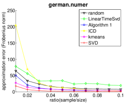
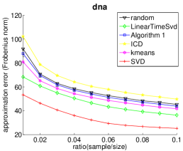
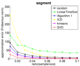
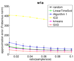
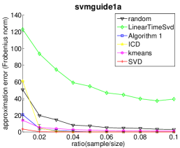
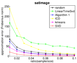
Figure 1: Nyström approximation errors for kernel matrices. The X-axis is the sampling ratio given as sample size divided by the matrix size. The Y-axis is the approximation error given in Frobenius norm. The tested algorithms are: random, LinearTimeSVD, Algorithm 1, ICD, k-means and SVD

7.2 General Matrices

We evaluate the performance of Algorithm 1 on general matrices by comparing it to a random choice of sub-sample. We use the full SVD as a benchmark that theoretically achieves the best accuracy. The approximation error is measured by $\left|\left|\hat{M}-M\right|\right|_{2}$.

The testing matrices in this section were chosen to have non-random spectra with random singular subspaces. Initially, a non-random diagonal matrix $L$ is chosen with non-increasing diagonal entries. $L$ will serve as the spectrum of our testing matrix. Then, two random unitary matrices $U$ and $V$ are generated. Our testing matrix is formed by $ULV^{T}$. We examine two degrees of spectrum decay: linear decay (slow) and exponential decay (fast).

The error is presented in $L_{2}$ norm and we vary the sample size to be between 1%-10% of the matrix size. The presented results are from an averaging of 20 iterations to reduce the statistical variability. For simplicity, we produce results only for $500\times 500$ square matrices.

The results are presented in Fig. 2. When the spectrum decays slowly, Algorithm 1 has no advantage over random sample selection. It produces overall pretty bad results. But the situation is much different in the presence of a fast spectrum decay. Algorithm 1 displays good results when the sample size allows it to capture most of the significant singular values of the data (at a sample rate of about 3%). It is interesting to note that random sample selection does not lag far behind. This hints that, on average, any sample is a good sample as long as it captures more data than the numeric rank of the matrix.

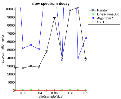
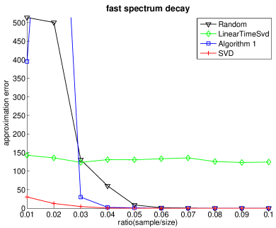
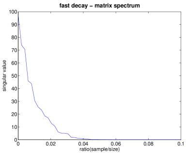
Figure 2: Nyström approximation errors for random matrices. The X-axis is the sampling ratio given as sample size divided by the matrix size. The Y-axis is the approximation error given in $L_{2}$ norm. The tested algorithms are Random, LinearTimeSVD, Algorithm 1 and SVD.

7.3 Non-Singularity of Sample Matrix

We empirically examine the relationship between the Nyström approximation error and the non-singularity of the sub-sample matrix. The approximation error is measured in $L_{2}$-norm and the non-singularity of $A_{M}\in\mathbb{R}^{s\times s}$ is measured by the magnitude of $\sigma_{s}\left(A_{M}\right)$. We employ testing matrices similar to those in section 7.2. These feature a non-random spectrum and random singular subspaces. The sample was chosen to be 5% of the data of the matrix. In this test, we compare between the random sample selection algorithm and Algorithm 1. Each algorithm ran 100 times on each matrix. The results of each run were recorded. Figure 3 features a log-log scale plot of the approximation error as a function of $\sigma_{s}\left(A_{M}\right)$. The performance of the different algorithm versions is compared. We arrive at similar conclusions to those in section 7.2. Our algorithms do no better than random sampling when the spectrum decay is slow, but consistently outperforms the random selection in the presence of fast spectrum decay. Figure 3 also shows a strong negative correlation between the variables in all the examined matrices. Hence, a large $\sigma_{s}\left(A_{M}\right)$ implies a small approximation error. The linear shape of the graphs, drawn in a log-log scale, suggests that this relationship is exponential. The results hint at a possible extension of the Nyström procedure to a Monte-Carlo method: Algorithm 1 can be run many times. In the end, we choose the sample for which $\sigma_{s}\left(A_{M}\right)$ is maximal.

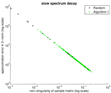
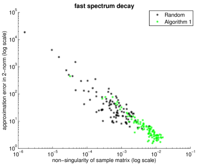
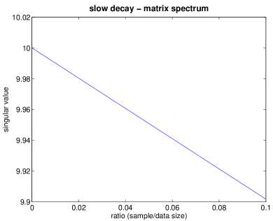
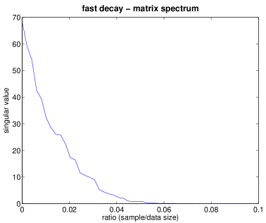
Figure 3: Errors in Nyström approximation as a function of $\sigma_{s}\left(A_{M}\right)$

8 Conclusion and Future Research

In this paper, we showed how the Nyström approximation method can be used to find the canonical SVD and EVD of a general matrix. In addition, we developed a sample selection algorithm that operates on general matrices. Experiments have been performed on real-world kernels and random general matrices. These show that the algorithm performs well when the spectrum of the matrix decays quickly and the sample is sufficiently large to capture most of the energy of the matrix (the number of non-zero singular values). Another experiment showed that the non-singularity of the sample matrix (as measured by the magnitude of the smallest singular value) is exponentially inversely related to the approximation error. This shows that our theoretical reasoning in Lemma 5.10 is qualitatively on par with empirical evidence.

Future research should focus on additional formalization of the relationship between the smallest singular value of the sample matrix and the Nyström approximation error. Another interesting possibility is to find a constrained class of matrices and develop a sample selection algorithm to take advantage of the constraint. Some classes of matrices may be easier to sub-sample with respect to the Nyström method.

References

• [1] D. Achlioptas, F. McSherry and B. Schölkopf, Sampling Techniques for Kernel Methods, Annual Advances in Neural Information Processing Systems 14, 2001.
• [2] C. T. H. Baker, The Numerical Treatment of Integral Equations, Oxford: Clarendon Press, 1977.
• [3] M. Bebendorf and R. Grzhibovskis, Accelerating Galerkin BEM for linear elasticity using adaptive cross approximation, Mathematical Methods in the Applied Sciences, Math. Meth. Appl. Sci., 29:1721-1747, 2006.
• [4] M. Bebendorf and S. Rjasanow, Adaptive Low-Rank Approximation of Collocation Matrices, Computing 70, 1-24, 2003.
• [5] S. Belongie, C. Fowlkes, F. Chung, and J. Malik, Spectral Partitioning with Indefinite Kernels Using the Nyström Extension, Proc. European Conf. Computer Vision, 2002.
• [6] Y. Bengio, O. Delalleau, N. Roux, J. Paiement, P. Vincent and M. Ouimet, Learning eigenfunctions links spectral embedding and kernel PCA. Neural Computation, 16, 2197-2219, 2004.
• [7] A. Bjorck and S. Hammarling, A Schur method for the square root of a matrix, Linear Algebra and Appl., 52/53 (1983) pp. 127-140.
• [8] P. A. Businger and G. H. Golub, Linear least squares solution by Householder transformation, Numerische Mathematik, 7 (1965), pp. 269-276.
• [9] E. J. Candes and T. Tao, The Power of Convex Relaxation: Near-Optimal Matrix Completion. IEEE Transactions on Information Theory, 56 (5). pp. 2053-2080.
• [10] C. C. Chang and C. J. Lin, LIBSVM : a library for support vector machines, 2001. Software available at http://www.csie.ntu.edu.tw/$\scriptstyle\sim$cjlin/libsvmtools/datasets/
• [11] R. R. Coifman and S. Lafon. Geometric harmonics: a novel tool for multiscale out-of-sample extension of empirical functions. Appl. Comp. Harm. Anal., 21(1):31-52, 2006.
• [12] T. Cox and M. Cox. Multidimensional scaling. Chapman & Hall, London, UK, 1994.
• [13] A. Deshpande and S. Vempala, Adaptive sampling and fast low-rank matrix approximation, Technical report TR06-042, Electronic Colloquium on Computational Complexity, 2006.
• [14] P. Drineas, R. Kannan and M. W. Mahoney, Fast Monte Carlo Algorithms for Matrices II: Computing a Low-Rank Approximation to a Matrix, SIAM J. Comput. 36(1), 158-183, 2006.
• [15] P. Drineas and M. W. Mahoney, On the Nyström method for approximating a Gram matrix for improved kernel-based learning, J. Machine Learning, 6, pp. 2153-2175, 2005.
• [16] S. Fine and K. Scheinberg. Efficient SVM training using low-rank kernel representations. J. Mach. Learn. Res., 2:243-264, 2001.
• [17] C. Fowlkes, S. Belongie, F. Chung, J. Malik, Spectral Grouping Using the Nyström Method, IEEE Transactions on Pattern Analysis and Machine Intelligence, vol. 26, no. 2, pp. 214-225, February, 2004.
• [18] C. Fowlkes, S. Belongie, and J. Malik, Efficient Spatiotemporal Grouping Using the Nyström Method, Proc. IEEE Conf. Computer Vision and Pattern Recognition, Dec. 2001.
• [19] G. H. Golub and C. F. Van Loan, Matrix Computations (3rd Ed.), Johns Hopkins University Press, 1996.
• [20] M. Gu, S. C. Eisenstat, An efficient algorithm for computing a strong rank revealing QR factorization, SIAM J. Sci. Comput., 17 (1996), pp. 848-869.
• [21] S. Har-Peled. Low rank matrix approximation in linear time. Manuscript. January 2006.
• [22] H. Hotelling. Analysis of a complex of statistical variables into principal components. Journal of Educational Psychology, 24:417-441, 1933.
• [23] S. Lafon and A. B. Lee. Diffusion maps and coarse-graining: A unified framework for dimensionality reduction, graph partitioning, and data set parameterization. IEEE Transactions on Pattern Analysis and Machine Intelligence, 28(9):1393-1403, 2006.
• [24] E. Liberty, F. Woolfe, P.-G. Martinsson, V. Rokhlin, and M. Tygert. Randomized algorithms for the low-rank approximation of matrices. Proc. Natl. Acad. Sci. USA, 104(51): 20167-20172, 2007.
• [25] M. Ouimet and Y. Bengio. Greedy spectral embedding. In Proceedings of the Tenth International Workshop on Artificial Intelligence and Statistics, 2005.
• [26] C. T. Pan. On the existence and computation of rank-revealing LU factorizations. Linear Algebra Appl, 316:199-222, 2000.
• [27] V. Rokhlin, A. Szlam, and M. Tygert, A randomized algorithm for principal component analysis, Tech. Rep. 0809.2274, arXiv, 2008. Available at http://arxiv.org.
• [28] S. T. Roweis and L. K. Saul. Nonlinear dimensionality reduction by Locally Linear Embedding. Science, 290(5500):2323-2326, 2000.
• [29] T. Sarlös, Improved approximation algorithms for large matrices via random projections, in Proceedings of the 47th Annual IEEE Symposium on Foundations of Computer Science, pp. 143-152, 2006
• [30] A. Smola and B. Schölkopf, Sparce greedy matrix approximation for machine learning, Proceedings of the 17th international conference on machine learning, pp 911-918. June, 2000.
• [31] G. W. Stewart, Four algorithms for the efficient computation of truncated QR approximations to a sparse matrix, Numer. Math., 83, pp. 313-323, 1999.
• [32] C. K. I. Williams and M. Seeger, Using the Nyström method to speed up kernel machines, Advances in Neural Information Processing Systems 2000, MIT Press, 2001.
• [33] K. Zhang, I. W. Tsang, and J. T. Kwok, Improved Nyström low-rank approximation and error analysis. In Proceedings of the 25th international Conference on Machine Learning (Helsinki, Finland, July 05 - 09, 2008). ICML ’08, vol. 307. ACM, New York, NY, 1232-1239, 2008.