Testability of the Higgs inflation scenario in a radiative seesaw model

Abstract

The Higgs inflation scenario is an approach to realize the inflation, in which the Higgs boson plays a role of the inflaton without introducing a new particle. We investigate a Higgs inflation scenario in the so-called radiative seesaw model proposed by E. Ma. We find that a part of parameter regions where additional scalar fields can play a role of an inflaton is compatible with the current LHC results, the current data from neutrino experiments and those of the dark matter abundance as well as the direct search. We show that we can partially test this model by measuring masses of scalar bosons at the International Linear Collider.

I Introduction

In 2012, the LHC discovered a new particle with the mass of 126 GeV atlas ; cms . The particle is regarded as the Higgs boson predicted in the Standard Model (SM) of elementary particles. The discovery of the Higgs boson means that all the particle contents in the SM are completed. The LHC is now searching for indications of new physics, and is trying to measure the deviation in the coupling from the SM. On the other hand, the cosmic observations such as the experiments at WMAP and Planck have reported the new results WMAP ; Planck . These experiments measure the temperature fluctuation of the cosmic microwave background precisely, by which we can impose constraints on the models of inflation. Cosmic inflation at the early Universe inf , which is a promising candidate to solve cosmological problems such as the horizon problem and the flatness problem, requires an additional scalar boson, the inflaton. We consider the Higgs inflation scenario where the Higgs boson plays a role of the inflaton. In the minimal model of this scenario Hinf , we do not have to introduce any other particle in addition to the particle contents in the SM to explain an inflation.

However, it would be difficult to realize the Higgs inflation scenario in the minimal model. Assuming the SM with one Higgs doublet, the vacuum stability argument indicates that the model can be well defined only below the energy scale where the running coupling of the Higgs self-coupling becomes zero. For the Higgs boson mass to be 126 GeV with the top quark mass to be 173.1 GeV and for the coupling for the strong force to be $\alpha_{s}=$ 0.1184, the critical energy scale is estimated to be around $10^{10}$ GeV using the NNLO calculation, although the uncertainty due to the values of the top quark mass and $\alpha_{s}$ is not small lambda_run . The vacuum seems to be metastable when we assume that the model holds up to the Planck scale. This kind of analysis gives a strong constraint on the scenario of the Higgs inflation, because the inflation occurs at the energy scale where the vacuum stability is not guaranteed in the SM. Recently, a viable model for the Higgs inflation has been proposed, in which the Higgs sector is extended including an additional scalar field other_Hinf ; 2Hinf . There is also another problem in the minimal model, which comes from unitarity argument uni_break ; uni_care .

Extending the Higgs sector from the SM one, we may expect to reveal new physics that can explain phenomena such as neutrino oscillation, existence of dark matter and baryon asymmetry of the Universe. Here, we extend the Higgs inflation model in the framework of a radiative seesaw scenario by E. Ma Kanemura:2012ha . The radiative seesaw scenario is a way to explain tiny neutrino masses, where they are radiatively induced at the loop level by introducing $Z_{2}$-odd scalar fields and $Z_{2}$-odd right-handed neutrinos KNT ; Ma ; AKS . An interesting characteristic feature in these radiative seesaw models is that dark matter candidates automatically enter into the model because of the $Z_{2}$ parity.

In this work, we discuss a simple model to explain inflation, neutrino masses and dark matter simultaneously, which is based on the simplest radiative seesaw model Ma . Both the Higgs boson and neutral components of the $Z_{2}$-odd scalar doublet can satisfy conditions on the slow-roll inflation slow-roll and vacuum stability up to the inflation scale. We find that a part of the parameter region where these scalar fields can play a role of the inflaton is compatible with the current LHC results, the current data from neutrino experiments and those of the dark matter abundance as well as the direct search XENON100 . A phenomenological consequence of scenario results in a specific mass spectrum of scalar fields, which can be tested at the International Linear Collider (ILC) ILC1 .

II Extension to a radiative seesaw model

We extend the Higgs inflation model in the framework of a radiative seesaw scenario Ma . In this model, there are the $Z_{2}$-odd scalar doublet field $\Phi_{2}$ and right-handed neutrino $\nu_{R}$ in addition to the $Z_{2}$-even SM Higgs doublet field $\Phi_{1}$ due to the invariance under the unbroken discrete $Z_{2}$ symmetry Ma . Because Dirac Yukawa couplings of neutrinos are forbidden by the $Z_{2}$ symmetry, the Yukawa interaction for leptons is given by ${\cal L}_{Yukawa}=Y_{\ell}\overline{L_{L}}\Phi_{1}\ell_{R}+Y_{\nu}\overline{L_{L}}\Phi_{2}^{c}\nu_{R}+h.c.$ (the superscript $c$ denotes the charge conjugation). The scalar potential is given by 2Hinf

$$V = \frac{M_{P}^{2}R}{2}+(\xi_{1}|\Phi_{1}|^{2}+\xi_{2}|\Phi_{2}|^{2})R+\mu_{1}^{2}|\Phi_{1}|^{2}+\mu_{2}^{2}|\Phi_{2}|^{2}$$ (1)

$$+\frac{1}{2}\lambda_{1}|\Phi_{1}|^{4}+\frac{1}{2}\lambda_{2}|\Phi_{2}|^{4}+\lambda_{3}|\Phi_{1}|^{2}|\Phi_{2}|^{2}+\lambda_{4}(\Phi_{1}^{\dagger}\Phi_{2})(\Phi_{2}^{\dagger}\Phi_{1})+\frac{1}{2}\lambda_{5}((\Phi_{1}^{\dagger}\Phi_{2})^{2}+h.c.),$$

where $M_{P}$($\simeq 10^{19}$ GeV) is the Planck scale, and $R$ is the Ricci scalar. Then, these quartic coupling constants should satisfy the following constraints on the unbounded-from-below conditions at the tree level;

$$\lambda_{1}>0,\ \ \lambda_{2}>0,\ \ \lambda_{3}+\lambda_{4}+\lambda_{5}+\sqrt{\lambda_{1}\lambda_{2}}>0,$$ (2)

and we impose the conditions of triviality;

$$\lambda_{i}\lesssim 2\pi.$$ (3)

Assuming $\mu_{1}^{2}<$0 and $\mu_{2}^{2}>$ 0, $\Phi_{1}$ obtains the vacuum expectation value (VEV) $v$ ($=\sqrt{-2\mu_{1}^{2}/\lambda_{1}}$), while $\Phi_{2}$ cannot get the VEV because of the unbroken $Z_{2}$ symmetry. The lightest $Z_{2}$-odd particle is stabilized by the $Z_{2}$ parity, and it can act as the dark matter as long as it is electrically neutral. Mass eigenstates of the scalar bosons are the SM-like $Z_{2}$-even Higgs scalar boson ($h$), the $Z_{2}$-odd CP-even scalar boson ($H$), the $Z_{2}$-odd CP-odd scalar boson ($A$) and $Z_{2}$-odd charged scalar bosons ($H^{\pm}$). Masses of these scalar bosons are given by Ma ; $m_{h}^{2}=\lambda_{1}v^{2},\ m_{H}^{2}=\mu_{2}^{2}+\frac{1}{2}(\lambda_{3}+\lambda_{4}+\lambda_{5})v^{2},\ m_{A}^{2}=\mu_{2}^{2}+\frac{1}{2}(\lambda_{3}+\lambda_{4}-\lambda_{5})v^{2},\ m_{H^{\pm}}^{2}=\mu_{2}^{2}+\frac{1}{2}\lambda_{3}v^{2}$.

III Constraints on the parameters

For the Higgs inflation scenario in our model defined in the previous section, there are nine parameters in the scalar sector; i.e., $\xi_{1}$, $\xi_{2}$, $\mu_{1}^{2}$, $\mu_{2}^{2}$, $\lambda_{1}$, $\lambda_{2}$, $\lambda_{3}$, $\lambda_{4}$ and $\lambda_{5}$. They must satisfy the vacuum stability condition on the running of the scalar coupling constants and the constraint from the slow-roll inflation, the dark matter data and the neutrino data. We find that a part of parameter regions is compatible with all constraints. Then, we can get the possible mass spectrum for additional scalar bosons in our model Kanemura:2012ha .

First, we discuss the constraint from the slow-roll inflation. In order that some of the scalar bosons play a role of the inflaton, we need to impose following conditions 2Hinf ;

$$\lambda_{2}\xi_{1}-(\lambda_{3}+\lambda_{4})\xi_{2} > 0,$$

$$\lambda_{1}\xi_{2}-(\lambda_{3}+\lambda_{4})\xi_{1} > 0,$$

$$\lambda_{1}\lambda_{2}-(\lambda_{3}+\lambda_{4})^{2} > 0.$$ (4)

Parameters in the scalar potential should satisfy the constraint from the power spectrum WMAP ; 2Hinf ;

$$\xi_{2}\sqrt{\frac{2(\lambda_{1}+a^{2}\lambda_{2}-2a(\lambda_{3}+\lambda_{4}))}{\lambda_{1}\lambda_{2}-(\lambda_{3}+\lambda_{4})^{2}}}\simeq 5\times 10^{4},\ \ \ \ \ \frac{\lambda_{5}}{\xi_{2}}\frac{a\lambda_{2}-(\lambda_{3}+\lambda_{4})}{\lambda_{1}+a^{2}\lambda_{2}-2a(\lambda_{3}+\lambda_{4})}\lesssim 4\times 10^{-12},$$ (5)

where $a$ is given as $a\equiv\xi_{1}/\xi_{2}$. When the scalar potential satisfies the conditions in Eqs. (4) and (5), the model could realize the inflation.

Second, we discuss the constraint from dark matter. We here assume that the CP-odd boson $A$ is the dark matter (the lightest $Z_{2}$-odd particle). When $\lambda_{5}$ is very small such as ${\cal O}(10^{-7})$, $A$ is difficult to act as the dark matter because the scattering process $AN\to HN$ ($N$ is a nucleon) opens and the cross section cannot be consistent with the current direct search results for dark matter direct_Z ; Kashiwase:2012xd ; LopezHonorez:2006gr . To avoid the process $AN\to HN$ kinematically, we here take $\lambda_{5}\simeq 10^{-6}$ and

$$a\lambda_{2}-(\lambda_{3}+\lambda_{4})\simeq 10^{-1}$$ (6)

at the inflation scale. With this choice, masses of $A$ and $H$ are almost the same value. The co-annihilation process $AH\to XX$ via the $Z$ boson is important to explain the abundance of the dark matter where $X$ is a particle in the SM, because the pair annihilation process $AA\to XX$ via the $h$ boson is suppressed due to the constraint from the inflation. Because the cross section of $AH\to XX$ depends only on the mass of the dark matter, the mass of the dark matter $A$ is constrained from the abundance of the dark matter as $128~{}{\rm GeV}\leq m_{A}\leq 138~{}{\rm GeV}$, where we have used the nine years WMAP data WMAP .

Third, we can explain tiny neutrino masses in this model which are generated by the one loop diagram Ma . The neutrino mass is related to $\lambda_{5}$ and masses of scalar bosons ($m_{H}$ and $m_{A}$), which are constrained from the inflation and the dark matter. From the relation $(Y_{\nu})_{i}^{k}(Y_{\nu})_{j}^{k}/M_{R}^{k}\simeq{\cal O}(10^{-11})$ GeV^-1 where $M_{R}^{k}$ is the Majorana mass of $\nu_{R}^{k}$ ($k$=1-3) and $(Y_{\nu})_{i}^{k}$ is neutrino Yukawa coupling constant, the magnitude of tiny neutrino masses can be explained. For example, when $M_{R}^{k}$ is ${\cal O}(1)$ TeV, $(Y_{\nu})_{i}^{k}$ is ${\cal O}(10^{-2})$.

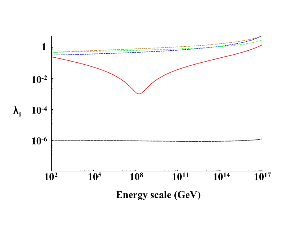
Figure 1: Running of the scalar coupling constants. Red (solid), blue (dashed), brown (dot-dashed), green (dotted) and black (long-dashed) curves show $\lambda_{1}$, $\lambda_{2}$, $\lambda_{3}$, $-\lambda_{4}$ and $\lambda_{5}$, respectively.

	$\lambda_{1}$	$\lambda_{2}$	$\lambda_{3}$	$\lambda_{4}$	$\lambda_{5}$
$10^{2}$ GeV	0.26	0.35	0.51	-0.51	1.0$\times 10^{-6}$
$10^{17}$ GeV	1.6	6.3	6.3	-3.2	1.2$\times 10^{-6}$

Table 1: The possible parameter set which satisfies constraints from the inflation and the dark matter at the scales of ${\cal O}(10^{2})$ GeV and ${\cal O}(10^{17})$ GeV.

Finally, we calculate the running of the coupling constants using the renormalization group equations beta . As shown in Fig 1, for the contribution of additional scalar bosons, this model can be stable up to the inflation scale from the electroweak scale extended_run . As numerical input parameters, we take the VEV ($v=246~{}$GeV), SM-like Higgs mass ($m_{h}=126$ GeV) and the allowed value for the dark matter mass ($m_{A}=130$ GeV). Further numerical input parameter comes from the perturbativity of $\lambda_{2}$ up to the inflation scale; i.e., $\lambda_{2}(\mu_{\rm inf})=2\pi$, where $\mu_{\rm inf}$ is the inflation scale $10^{17}$ GeV. The parameter set in Table 1 can be consistent with these numerical inputs and the constraints are given in Eqs. (2)-(6). Consequently, we can obtain the mass spectrum of the scalar bosons in our model as

$$m_{h}\simeq 126~{}{\rm GeV},\ \ \ m_{H^{\pm}}\simeq 173~{}{\rm GeV},\ \ \ m_{H}\simeq 130~{}{\rm GeV},\ \ \ m_{A}\simeq 130~{}{\rm GeV},$$ (7)

where the mass difference between $A$ and $H$ is about 500 KeV. The mass spectrum is not largely changed even if $m_{A}$ is varied with in its allowed region. In the next section, we consider the constraints on our model from the existing experiments and the way to test the characteristic mass spectrum in this model at the future collider experiment.

IV Phenomenology

The LEP experiment constrains masses of the $Z_{2}$-odd scalar bosons. The mass of charged scalar bosons $m_{H^{\pm}}$ should be lager than 70-90 GeV by the LEP LEP_direct ; LEP_pm . This constraint is satisfied in our model ($m_{H^{\pm}}\simeq 173~{}{\rm GeV}$). Furthermore, $m_{H}+m_{A}$ should be larger than $m_{Z}$, and the combination of $m_{H}$ and $m_{A}$ is bounded by $H$$A$ production by the LEP date LEP_direct ; LEP_HApair . However, when $m_{H}-m_{A}<8$ GeV, masses of neutral $Z_{2}$-odd scalar boson loop diagrams are not really constrained by the LEP LEP_direct ; LEP_HApair . On the other hand, the contributions to the electroweak parameters STdef from additional scalar bosons loops which are given by ST1 ; ST2 are also consistent with the electroweak precision data with 90% Confidence Level (C.L.) ST2 .

Next, we consider the way to test at the LHC. According to Refs. LHC1 ; LHC2 ; LHC3 , they conclude that it could be difficult to test $pp\to AH^{+}/HH^{+}/H^{+}H^{-}$ processes because the cross sections of the background processes are very large. The process of $pp\to AH$ could be tested with about the 3$\sigma$ C.L. with the various benchmark points for $m_{A}$ and $m_{H}$. However, it would be difficult to test $pp\to AH$ in our scenario, because $m_{H}$ and $m_{A}$ are almost degenerate in our scenario, and the event number of $pp\to AH$ is negligibly small after imposing the basic cuts LHC1 ; LHC2 ; LHC3 . Furthermore, as the total decay width of $H$ is about $10^{-29}$ GeV, $H$ would pass through the detector. Therefore, this signal is also difficult to be detected at the LHC.

Finally, we discuss the signals of $H,A$ and $H^{\pm}$ at the ILC with $\sqrt{s}=500$ GeV. In the following, we use Calchep 2.5.6 for numerical evaluation calc . We focus on the $H^{\pm}$ pair production process: $e^{+}e^{-}\to Z^{*}(\gamma^{*})\to H^{+}H^{-}\to W^{+(*)}W^{-(*)}AA\to jj\ell\nu AA$ ($j$ denotes a hadron jet) ILC2 . Because of the kinematical reason, the energy of the two-jet system $E_{jj}$ satisfies the following equation;

$$\frac{m_{H^{\pm}}^{2}-m_{A}^{2}}{\sqrt{s}+2\sqrt{s/4-m_{H^{\pm}}^{2}}}<E_{jj}<\frac{m_{H^{\pm}}^{2}-m_{A}^{2}}{\sqrt{s}-2\sqrt{s/4-m_{H^{\pm}}^{2}}}.$$ (8)

In our parameter set, the distribution of $E_{jj}$ for the differential cross section in this process is shown in Fig. 2.

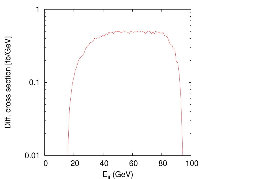
Figure 2: The distribution of $E_{jj}$ for the differential cross section for $e^{+}e^{-}\to H^{+}H^{-}\to W^{+(*)}W^{-(*)}AA\to jj\ell\nu AA$. In our parameter set, the endpoint of $E_{jj}$ is estimated at $15~{}{\rm GeV}<E_{jj}<94~{}{\rm GeV}$.

The important background processes against this process, which are $e^{+}e^{-}\to W^{+}W^{-}\to jj\ell\overline{\nu}$ and $e^{+}e^{-}\to Z(\gamma)Z\to jj\ell\overline{\ell}$ with a missing $\overline{\ell}$ event, could be well reduced by imposing an appropriate kinematic cuts. Then, we expect that $m_{H^{\pm}}$ and $m_{A}$ can be measured by using the endpoints of $E_{jj}$ at the ILC after the background reduction.

On the other hand, we consider $HA$ production: $e^{+}e^{-}\to Z^{*}\to HA\to AAZ^{*}\to AAjj$ at the ILC. If the mass difference between $m_{A}$ and $m_{H}$ is sizable, it could also be detected by using the endpoint of $E_{jj}$. However, $m_{A}$ and $m_{H}$ are almost degenerate in our scenario. When we detect $H^{\pm}$ but we cannot detect the clue of this process at the ILC, it seems that $m_{A}$ and $m_{H}$ are almost same value.

V Conclusion

We have studied the Higgs inflation model in the framework of a radiative seesaw scenario. In our model, we may be able to explain inflation, neutrino masses and dark matter simultaneously. We find that a part of parameter regions is compatible with all constraints which come from the conditions of the slow-roll inflation, the current LHC results, the current data from neutrino experiments and those of the dark matter abundance as well as the direct search results. We can test this scenario by measuring masses of scalar bosons at the ILC with $\sqrt{s}=500$ GeV.

- (1) S. Kanemura, T. Matsui, T. Nabeshima and , arXiv:1211.4448 [hep-ph].
- (2) G. Aad et al. [ATLAS Collaboration], Phys. Lett. B 716 (2012) 1.
- (3) S. Chatrchyan et al. [CMS Collaboration], Phys. Lett. B 716 (2012) 30.
- (4) D. Larson et al., Astrophys. J. Suppl. 192 (2011) 16, G. Hinshaw, D. Larson, E. Komatsu, D. N. Spergel, C. L. Bennett, J. Dunkley, M. R. Nolta and M. Halpern et al., arXiv:1212.5226 [astro-ph.CO].
- (5) P. A. R. Ade et al. [ Planck Collaboration], arXiv:1303.5062 [astro-ph.CO].
- (6) A. H. Guth, Phys. Rev. D 23 (1981) 347; K. Sato, Mon. Not. Roy. Astron. Soc. 195 (1981) 467.
- (7) F. L. Bezrukov and M. Shaposhnikov, Phys. Lett. B 659 (2008) 703.
- (8) A. De Simone, M. P. Hertzberg and F. Wilczek, Phys. Lett. B 678 (2009) 1; F. Bezrukov and M. Shaposhnikov, JHEP 0907 (2009) 089; J. Elias-Miro, J. R. Espinosa, G. F. Giudice, G. Isidori, A. Riotto and A. Strumia, Phys. Lett. B 709 (2012) 222; G. Degrassi, S. Di Vita, J. Elias-Miro, J. R. Espinosa, G. F. Giudice, G. Isidori and A. Strumia, JHEP 1208 (2012) 098.
- (9) R. N. Lerner and J. McDonald, Phys. Rev. D 80 (2009) 123507,R. N. Lerner and J. McDonald, Phys. Rev. D 83 (2011) 123522,R. N. Lerner and J. McDonald, JCAP 1211 (2012) 019,C. Arina, J. -O. Gong and N. Sahu, Nucl. Phys. B 865 (2012) 430.
- (10) J. -O. Gong, H. M. Lee and S. K. Kang, JHEP 1204 (2012) 128.
- (11) C. P. Burgess, H. M. Lee and M. Trott, JHEP 0909 (2009) 103; JHEP 1007 (2010) 007; J. L. F. Barbon and J. R. Espinosa, Phys. Rev. D 79 (2009) 081302; M. P. Hertzberg, JHEP 1011 (2010) 023.
- (12) G. F. Giudice and H. M. Lee, Phys. Lett. B 694 (2011) 294.
- (13) L. M. Krauss, S. Nasri and M. Trodden, Phys. Rev. D 67 (2003) 085002; K. Cheung and O. Seto, Phys. Rev. D 69 (2004) 113009.
- (14) E. Ma, Phys. Rev. D 73 (2006) 077301; Phys. Lett. B 662 (2008) 49; T. Hambye, K. Kannike, E. Ma and M. Raidal, Phys. Rev. D 75 (2007) 095003; E. Ma and D. Suematsu, Mod. Phys. Lett. A 24 (2009) 583.
- (15) M. Aoki, S. Kanemura and O. Seto, Phys. Rev. Lett. 102 (2009) 051805; Phys. Rev. D 80 (2009) 033007; M. Aoki, S. Kanemura and K. Yagyu, Phys. Rev. D 83 (2011) 075016; Phys. Lett. B 702 (2011) 355.
- (16) A. D. Linde, Phys. Lett. B 108 (1982) 389; A. Albrecht and P. J. Steinhardt, Phys. Rev. Lett. 48 (1982) 1220.
- (17) E. Aprile et al. [XENON100 Collaboration], Phys. Rev. Lett. 109 (2012) 181301.
- (18) J. Brau, (Ed.) et al. [ILC Collaboration], arXiv:0712.1950 [physics.acc-ph]; G. Aarons et al. [ILC Collaboration], arXiv:0709.1893 [hep-ph]; N. Phinney, N. Toge and N. Walker, arXiv:0712.2361 [physics.acc-ph]; T. Behnke, (Ed.) et al. [ILC Collaboration], arXiv:0712.2356 [physics.ins-det]; H. Baer, et al. ”Physics at the International Linear Collider”, Physics Chapter of the ILC Detailed Baseline Design Report: http://lcsim.org/papers/DBDPhysics.pdf.
- (19) Y. Cui, D. E. Morrissey, D. Poland and L. Randall, JHEP 0905 (2009) 076; C. Arina, F. -S. Ling and M. H. G. Tytgat, JCAP 0910 (2009) 018.
- (20) S. Kashiwase and D. Suematsu, Phys. Rev. D 86 (2012) 053001.
- (21) L. Lopez Honorez, E. Nezri, J. F. Oliver and M. H. G. Tytgat, JCAP 0702 (2007) 028.
- (22) K. Inoue, A. Kakuto and Y. Nakano, Prog. Theor. Phys. 63 (1980) 234; H. Komatsu, Prog. Theor. Phys. 67 (1982) 1177.
- (23) S. Nie and M. Sher, Phys. Lett. B 449 (1999) 89; S. Kanemura, T. Kasai and Y. Okada, Phys. Lett. B 471 (1999) 182.
- (24) G. Abbiendi et al. [OPAL Collaboration], Eur. Phys. J. C 35 (2004) 1; Eur. Phys. J. C 32 (2004) 453.
- (25) A. Pierce and J. Thaler, JHEP 0708 (2007) 026.
- (26) E. Lundstrom, M. Gustafsson and J. Edsjo, Phys. Rev. D 79 (2009) 035013.
- (27) M. E. Peskin and T. Takeuchi, Phys. Rev. Lett. 65 (1990) 964; Phys. Rev. D 46 (1992) 381.
- (28) D. Toussaint, Phys. Rev. D 18 (1978) 1626; M. E. Peskin and J. D. Wells, Phys. Rev. D 64 (2001) 093003.
- (29) S. Kanemura, Y. Okada, H. Taniguchi and K. Tsumura, Phys. Lett. B 704 (2011) 303; M. Baak, M. Goebel, J. Haller, A. Hoecker, D. Ludwig, K. Moenig, M. Schott and J. Stelzer, Eur. Phys. J. C 72 (2012) 2003.
- (30) R. Barbieri, L. J. Hall and V. S. Rychkov, Phys. Rev. D 74 (2006) 015007 [hep-ph/0603188].
- (31) Q. -H. Cao, E. Ma and G. Rajasekaran, Phys. Rev. D 76 (2007) 095011.
- (32) E. Dolle, X. Miao, S. Su and B. Thomas, Phys. Rev. D 81 (2010) 035003
- (33) A. Pukhov, hep-ph/0412191.
- (34) M. Aoki, S. Kanemura and H. Yokoya, arXiv:1303.6191 [hep-ph]; M. Aoki and S. Kanemura, Phys. Lett. B 689 (2010) 28.