Reconstruction of Tip-Surface Interactions with Multimodal Intermodulation Atomic Force Microscopy

Abstract

We propose a theoretical framework for reconstructing tip-surface interactions using the intermodulation technique when more than one eigenmode is required to describe the cantilever motion. Two particular cases of bimodal motion are studied numerically: one bending and one torsional mode, and two bending modes. We demonstrate the possibility of accurate reconstruction of a two-dimensional conservative force field for the former case, while dissipative forces are studied for the latter.

I Introduction

Atomic force microscopy Binnig et al. (1986) (AFM) has become one of the most important tools for the study of nanometer-scale surface properties of a wide range of materials. The initial goal of AFM was surface topography imaging which was performed by scanning a cantilever with a sharp tip over a surface while keeping its deflection constant. It was later realized that the reconstruction of tip-surface interactions was possible and that these interactions contain valuable information about material properties Burnham et al. (1993); Butt et al. (2005). One of the first reconstruction methods was based on measurement of the quasi-static bending of the cantilever beam as its base was slowly moved toward and away from the surface. Two drawbacks of this method are the slow speed of measurement and the lack of ability to reconstruct dissipative forces which are always present in tip-surface interactions due to non-elastic deformations of the sample, breaking chemical bonds, or other irreversible processes Hoffmann et al. (2001); García et al. (2006a); Negri et al. (2010); Saitoh et al. (2010); She and Balatsky (2012).

The development of dynamic AFM opened new pathways for a more profound study of tip-surface interactions. In dynamic AFM the cantilever is treated as an underdamped oscillator (high $Q$-factor) driven at a resonance where the response to external forces is enhanced by a factor $Q$. A large number of methods for determining the tip-surface interaction have been devised Krotil et al. (1999); García and Perez (2002); Giessibl (2003); Sader et al. (2005); Albers et al. (2009); Gross et al. (2009); Solares and Chawla (2010), some making use of amplitude or frequency modulation Albrecht et al. (1991); Stark et al. (2002); Legleiter et al. (2006); Lee and Jhe (2006); Jesse et al. (2007); Sahin et al. (2007); Rodriguez et al. (2007); Labuda et al. (2011); Sarioglu et al. (2012); Serra-García et al. (2012). In this paper, we consider intermodulation AFM (ImAFM) Platz et al. (2008) which is unique in its ability to rapidly extract a large amount of information about tip-surface interactions in a simple and convenient way Hutter et al. (2010); Forchheimer et al. (2012). With ImAFM we have the possibility of high resolution surface property mapping at interactive scan speeds and reconstruction of the tip-surface interaction at each pixel.

The main idea underlying ImAFM is to use the nonlinear tip-surface forces to create high-order intermodulation of discrete tones in a frequency comb Helmholtz (1895). The method can be generally applied to any resonator subject to a nonlinear force when it is driven with at least two frequencies $\omega_{d1}$ and $\omega_{d2}$. The nonlinear response in frequency domain occurs not only at the drive frequencies and their harmonics $n\omega_{d1}$ and $m\omega_{d2}$, where $n$ and $m$ are integers, but also at their linear combinations $\omega=n\omega_{d1}+m\omega_{d2}$ or intermodulation products. Due to the signal enhancement near resonance and finite detector noise of the measurement, a typical spectrum of cantilever motion can be obtained only in narrow frequency band near resonance. Concentrating as many intermodulation products as possible in this resonant detection band results in more information for reconstruction of the nonlinear forces (fig. 1).

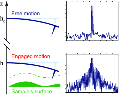
Figure 1: (Color online) Appearance of new frequencies in the spectrum of the tip motion in ImAFM due to the nonlinearities in tip-surface interaction. The dashed line shows the characteristic range of the tip-surface force.

The sensitivity enhancement of dynamic AFM occurs not only at one single eigenmode, but also at several eigenmodes simultaneously. Measurement of the sample response at higher frequencies allows for better material imaging contrasts and improves accuracy of the tip-surface force reconstruction Stark and Heckl (2000); Proksch (2006); Martinez et al. (2006); Rupp et al. (2007); Lozano and García (2008); Lozano and Garcia (2009); Martinez-Martin et al. (2011). If we also excite a torsional resonance of the cantilever we open up the possibility of measuring lateral forces acting on the tip Yurtsever et al. (2008); Hakari et al. (2011); Bulgarevich et al. (2007). Additionally, when driving the cantilever at more than one eigenmode, new frequency bands become available for collecting intermodulation products, resulting from the nonlinear force which couples multiple eigenmodes Gigler et al. (2012). While ImAFM has been well studied for the case of one flexural mode Hutter et al. (2010); Forchheimer et al. (2012); Platz et al. (2013a, b, c), the multi-eigenmode problem remains open. In the current investigation we explore the possibility of reconstructing two-dimensional tip-surface force fields using two collinear eigenmodes (e.g. two flexural or two torsional modes) as well as two orthogonal modes (e.g. one flexural and one torsional mode).

The paper is organized as follows: in section II we consider general properties of the cantilever model and tip-surface interactions. In section III we recount the main principles of ImAFM, demonstrate how to obtain intermodulation spectra of tip-surface forces, and develop an extension of the spectral fitting method Hutter et al. (2010); Forchheimer et al. (2012) of force reconstruction for the multimodal case. In Section IV numerical results for the reconstruction of two-dimensional conservative and dissipative forces are presented. Section V concludes with a discussion and summary.

II Model

In order to proceed with the multimodal problem we should start from some general discussion of cantilever dynamics Raman et al. (2008); Rabe et al. (1996). If we are interested in studying only flexural modes, one-dimensional Euler-Bernoulli beam theory Lee et al. (2002); Rodriguez and García (2002); Melcher et al. (2007); Sader (1998) is sufficient. Incorporating torsional modes requires the cantilever to be regarded as a two-dimensional object. Many theories have been developed describing the continuum mechanics of two-dimensional plates Love (1888); Timoshenko and Woinowsky-Krieger (1959); Reddy (2007); Reissner and Stein (1951). A general description of an arbitrary two-dimensional cantilever (fig. 2) is given by the governing equation

$$\left(\mathcal{G}_{xy}+\mathcal{G}_{t}\right)\left[w\left(x,y,t\right)\right]=F+\mathrm{f}$$ (1)

with an appropriate set of boundary conditions.

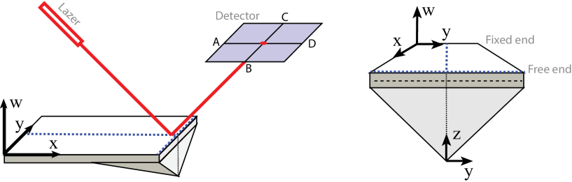
Figure 2: (Color online) Schematic representation of the two-dimensional cantilever and detection principle in AFM.

Here $x$ and $y$ are the two space coordinates, $t$ is time, $w(x,y,t)$ is a deflection normal to the $x-y$ plane of the plate at rest, $\mathcal{G}_{xy}$ is a space coupling operator which corresponds to the two-dimensional mathematical model used to determine the stresses and deformations in thin plates, and $\mathcal{G}_{t}$ is a time evolution operator which represents inertia and damping. $F$ and $\mathrm{f}$ are a scalar quantities which are projections on to $w$, of the two-dimensional vector force field acting on the tip, and the drive, respectively. In general, the force $F$ can depend explicitly on the deflection $w$, its velocity $\dot{w}$, past trajectories $\left.\{w,\dot{w}\}\right|_{-\infty}^{t}$ and time $t$. In this paper we restrict ourselves to $F$ which are not dependent on past trajectories. We consider only the case of small deflections, so $\mathcal{G}_{xy}$ and $\mathcal{G}_{t}$ are linear. For example, within the Kirchhoff-Love plate theory Love (1888) the space operator for a homogeneous cantilever reads

$$\mathcal{G}_{xy}:=\frac{2h^{3}E}{3(1-\nu^{2})}\left(\frac{\partial^{4}}{\partial x^{4}}+2\frac{\partial^{4}}{\partial x^{2}\partial y^{2}}+\frac{\partial^{4}}{\partial y^{4}}\right)$$ (2)

where $2h$ is the cantilever thickness, $E$ the Young’s modulus and $\nu$ the Poisson’s ratio. The theory assumes that a mid-surface plane can be used to represent a three-dimensional plate in a two-dimensional form. The time evolution operator $\mathcal{G}_{t}$ consists of an inertial term, and for the case of a homogeneous viscous media, a linear damping term

$$\mathcal{G}_{t}:=2\rho h\frac{\partial^{2}}{\partial t^{2}}+2\gamma\frac{\partial}{\partial t}$$ (3)

where $\rho$ is the cantilever density and $\gamma$ a damping coefficient.

The linearity of $\mathcal{G}_{xy}$ and $\mathcal{G}_{t}$ gives a dynamics of the two-dimensional cantilever which is well approximated by a system of differential equations for the generalized coordinates $q_{i}$ representing deflections of its normal modes (see appendix A for a derivation)

$$k_{i}\left(\frac{1}{\omega_{i}^{2}}\ddot{q}_{i}+\frac{1}{Q_{i}\omega_{i}}\dot{q}_{i}+q_{i}\right)=F_{i}\left(t\right)+\mathrm{f}_{i}\left(t\right)$$ (4)

Here each generalized coordinate $q_{i}$ has a stiffness $k_{i}$, resonant frequency $\omega_{i}$ and quality factor $Q_{i}$. $F_{i}(t)$ is the projection of the nonlinear force and $\mathrm{f}_{i}(t)$ is the projection of the drive force on to the $i^{\mathrm{th}}$ eigenmode. The problem of mapping the eigenmode coordinates $q_{i}$ onto the physical position of the tip $\mathbf{r}\equiv(z,y)^{\intercal}$, (hereafter $\intercal$ denotes transpose) as well as the relationship between $F_{i}$ and the actual vector force field acting on the tip $\mathbf{F}_{ts}(\mathbf{r},\dot{\mathbf{r}})$, is determined by the cantilever and tip geometry as briefly discussed in section IV.

III Reconstructing force from intermodulation with multiple eigenmodes

We recall the basic steps to get information about $F_{i}$ in the frequency domain using the intermodulation technique. Firstly, we excite one or several generalized coordinates (4) with the drive $\mathrm{f}_{i}$ and measure its motion spectrum at the height $h_{0}$, far from the sample surface, so $\left.\hat{F}_{i}\right|_{h_{0}}\equiv 0$ for all $t$. This free oscillation spectrum is denoted

$$\left.\hat{q}_{i}\right|_{h_{0}}=\chi_{i}\hat{\mathrm{f}}_{i}$$ (5)

where the hat represents the discrete Fourier transform (DFT)

$$\hat{q}(\omega)\equiv\mathcal{F}[q(t)]:=\sum\limits_{m=-\infty}^{\infty}q(t)e^{-2\pi\imath m\,\delta\omega t}$$ (6)

and the linear response function $\chi_{i}$ is introduced

$$\chi_{i}(\omega)=k_{i}^{-1}\left[1+\frac{\imath}{Q_{i}}\left(\frac{\omega}{\omega_{i}}\right)-\left(\frac{\omega}{\omega_{i}}\right)^{2}\right]^{-1}$$ (7)

Using pairs of drive tones with the same amplitude $A_{i}$ which are separated by $\delta\omega$ and placed close to each resonance $n_{i}\delta\omega<\omega_{i}<(n_{i}+1)\delta\omega$, where $n_{i}$ is an integer,

$$\mathrm{f}_{i}(t)=A_{i}\left[\cos\left(n_{i}\delta\omega t\right)+\cos\left((n_{i}+1)\delta\omega t\right)\right]$$ (8)

we obtain a free, linear response spectrum (eq. (5)) consisting components only at the drive frequencies $\omega_{i}\pm\delta\omega/2$ (fig. 1). Data acquisition in ImAFM should be performed over at least one total period of the drive $T=2\pi/\delta\omega$ while measuring subsequent periods only improves the SNR of the measured spectra Tholén et al. (2011); ima .

We then we move the cantilever closer to the sample to the engaged height $h$, so the oscillating tip starts to feel interaction with a surface (but not too close, so that there is zero static deflection of the cantilever) and measure the motion spectrum again

$$\left.\hat{q}_{i}\right|_{h}=\chi_{i}\left(\hat{F}_{i}+\hat{\mathrm{f}}_{i}\right)$$ (9)

Finally, the difference between this engaged motion spectrum (9) and free motion spectrum (5) yields the desired interaction force spectrum

$$\hat{F}_{i}=\chi_{i}^{-1}\left(\left.\hat{q}_{i}\right|_{h}-\left.\hat{q}_{i}\right|_{h_{0}}\right)\equiv\chi_{i}^{-1}\Delta\hat{q}_{i}$$ (10)

where finite difference operator $\Delta$ is used for short. Thus, we have obtained information about $F_{i}$ in the frequency space representation of the motion and we are in a position to discuss the reconstruction of its dependence on generalized coordinates $q_{i}$ and velocities $\dot{q}_{i}$.

Under ideal conditions, given the full difference spectrum $\Delta\hat{q}_{i}$ and corresponding response function $\chi_{i}$, it is possible to find $F_{i}(t)$ as the inverse Fourier transform of $\hat{F}_{i}(\omega)$ and then trivially recover its coordinate dependence $F_{i}(\{q_{i},\dot{q}_{i}\})$ using the measured motion $q_{i}(t)$. However, in real experiments this naïve approach fails due to the strong frequency dependence of $\chi_{i}$ and the measurement limitations imposed by detection noise. In practice, almost all of the spectrum $\hat{q}_{i}$ is buried under detector noise except for a narrow band near its resonant frequency where the signal-to-noise ratio (SNR) meets the thermal limit. Usually the number of resolvable spectral components $B_{i}$ in a band surrounding each eigenmode resonance is limited to a few dozen, depending on the difference frequency $\delta\omega$ and the forces experienced during the interaction. The use of several ($N$) eigenmodes allows for a lager total number of frequency components $B=\sum_{i=1}^{N}B_{i}$ for force reconstruction.

Different methods have been elaborated for the single mode reconstruction problem using this limited amount of response in the resonant detection band Hutter et al. (2010); Forchheimer et al. (2012); Platz et al. (2013a, b, c). Here we develop an extension of the spectral fitting method Hutter et al. (2010); Forchheimer et al. (2012); Platz et al. (2013c) for the multimodal problem as it allows for a straightforward generalization without involving any sophisticated concepts Platz et al. (2013a). Following the method’s main idea, one assumes a tip-surface force in the form of some known model function $\tilde{F}_{i}(q_{1},\dots,q_{N};\mathbf{g})$ with a vector $\mathbf{g}=(g_{1},\dots\,g_{P})^{\intercal}$ of $P$ unknown parameters. Fitting the calculated spectrum $\hat{\tilde{F}}_{i}(\omega)$ to the measured $\hat{F}_{i}(\omega)$ (eq. (10)), we minimize the error function in the frequency domain, in a least square sense

$$\begin{array}[]{lcl}\min\limits_{\mathbf{g}}\hat{e}_{i}=\hat{F}_{i}-\hat{\tilde{F}}_{i}\left(q_{1},\dots,q_{N};\mathbf{g}\right)\end{array}$$ (11)

The model $\tilde{F}_{i}$ can be a particular phenomenological expression, for example the van der Waals-Derjagin-Muller-Toporov (vdW-DMT) force Derjaguin et al. (1975) or its modifications García et al. (2006b); Gotsmann et al. (1999); Melcher et al. (2008). However, in the general case we do not know the exact form of the interaction and should choose some generic function structure, for instance a truncated Taylor expansion in the following polynomial form

$$\tilde{F}_{i}(q_{1},\dots,q_{N})=\sum\limits_{i_{1}=0}^{P_{1}}\dots\sum\limits_{i_{N}=0}^{P_{N}}g_{i_{1}\dots i_{N}}q_{1}^{i_{1}}\dots q_{N}^{i_{N}}=\mathbf{q}^{\intercal}\mathbf{g}$$ (12)

Here $P_{i}$ is the degree of the polynomial in $q_{i}$, $\mathbf{q}$ and $\mathbf{g}$ are vectors of basis functions and parameters respectively, each being of size $P=\prod_{i=1}^{N}P_{i}$

$$\begin{array}[]{lcl}\mathbf{q}=\left(1,\ q_{1},\ q_{1}^{2},\ \dots,\ q_{2},\ q_{1}q_{2},\ q_{1}^{2}q_{2},\ \dots\right)^{\intercal}\\ \mathbf{g}=\left(g_{00\dots},\ g_{10\dots},\ g_{20\dots},\ \dots,\ g_{01\dots},\ g_{11\dots},\ g_{21\dots},\ \dots\right)^{\intercal}\end{array}$$ (13)

Although the polynomial model is more universal, it usually contains a much larger number of unknown parameters which do not directly correspond to physical properties of the material or surface.

Inserting (12) into equation (10), we obtain a system of linear equations for the polynomial coefficients $g_{i_{1}\dots i_{N}}$ which is conveniently represented in matrix notation

$$\mathbf{g}=\mathbf{\hat{H}}^{+}\mathbf{\hat{F}}_{i}$$ (14)

where $\mathbf{\hat{H}}$ is a $B\times P$ matrix with rows $\hat{H}_{k}=\mathcal{F}_{k}[\mathbf{q}^{\intercal}]$ ($k$ is the corresponding component of the discrete Fourier transform of $\mathbf{q}$), $\mathbf{\hat{H}}^{+}$ its Moore-Penrose pseudoinverse, and $\mathbf{\hat{F}}_{i}$ a vector of size $B$. Note that total number of unknown parameters $P$ can not be greater than $B$ and in the case of an overdetermined system ($P<B$) the pseudoinverse will give a unique solution to (12) in a least square sense (11). Reconstruction of the velocity-dependent part of the force $F_{i}$ can be performed in the same way as for a conservative force, by polynomial expansion in $\dot{q}_{i}$ with corresponding coefficients.

IV Reconstruction of two-dimensional tip-surface forces from intermodulation AFM spectra

Thus the reconstruction of tip-surface force from multiple eigenmodes is a straight-forward generalization of the single eigenmode problem, albeit with the complication of keeping track of multiple modes and the possibility that tones can intermodulate between these modes. From an algebraic point of view the spectral fitting method can be regarded as a multivariate interpolation Jetter et al. (2006) and the simplest model which is linear in the parameters suffers from Runge’s phenomena Schl milch et al. (1901); Dahlquist and Björk (1974) when high-order nonlinearities couple the multiple eigenmode coordinates. Furthermore, reconstruction from many eigenmodes is a multi-dimensional problem with many model parameters and it will ultimately suffer from the need to either calibrate or determine these parameters from the limited number of intermodulation products that can be extracted from the narrow frequency bands near the resonances.

In a real experiment, the AFM detector is typically not able measure over a frequency range which covers many eigenmodes of the cantilever. Furthermore, the AFM detector is only capable of measuring two signals, corresponding to two orthogonal motions of the cantilever, that of flexing and twisting. The case of only two eigenmodes is therefore a reasonable simplification of the multi-modal problem which of great practical interest. In the following we restrict ourselves to this bimodal case.

We are interested in reconstruction of the two-dimensional tip-surface vector force field $\mathbf{F}_{ts}(\mathbf{r},\dot{\mathbf{r}})$ which depends on the physical tip position in the $y-z$ plane, $\mathbf{r}=(z,y)^{\intercal}$. Before we proceed with the two-mode analysis we should map the set of forces $F_{i}$ acting on the cantilever eigenmodes $q_{i}$ onto the physical force $\mathbf{F}_{ts}$. With this aim, we can transform the basis set for defining $q_{i}$ to separate ”pure” modes from ”mixed” modes. Applying some transformation, the exact form of which depends on the geometrical shape of the cantilever, we obtain the pure eigencoordinates $z_{i}$ and $y_{i}$ contributing only to the tip position perpendicular and parallel to the surface respectively. Here the two different $z_{i}$ (or $y_{i}$) are collinear while $z_{i}$ and $y_{i}$ are orthogonal. The remaining $\mathbf{q}^{\times}_{i}$ are mixed eigencoordinates of the cantilever, or cross-modes contributing to both coordinates $z$ and $y$ simultaneously, so that

$$\begin{array}[]{lcl}z=\sum z_{i}+\sum\mathbf{q}^{\times}_{i}\cdot\mathbf{z}\\ y=\sum y_{i}+\sum\mathbf{q}^{\times}_{i}\cdot\mathbf{y}\end{array}$$ (15)

Here the second terms are projections of the mixed eigencoordinates onto the tip coordinate system $(\mathbf{z},\mathbf{y})$. In doing so, the force $\mathbf{F}_{ts}$ is projected onto the $(\mathbf{z},\mathbf{y})$ so that its components parallel to the surface $F_{z}$ and perpendicular to the surface $F_{y}$ act on the corresponding pure modes, i.e. $F_{i}=F_{z}$ for each $z_{i}$, $F_{i}=F_{y}$ for each $y_{i}$, and different force projections act on the mixed modes.

Simultaneous excitation of the several pure eigenmodes coupled by nonlinear tip-surface interaction leads to excitation of the mixed modes which allows for measurements of the response in additional frequency bands. Although it would provide additional information, in this paper we investigate the simplest multimodal motion, that of pure bimodal motion without considering the cross-modes. In this case, analysis of the cantilever dynamics reduces to study of two characteristic regimes: bimodal motion of the collinear eigencoordinates (e.g. two flexural or torsional modes) and orthogonal eigencoordinates (one flexural and one torsional mode). Let us proceed with the former.

IV.1 Case 1: Two collinear modes

This case corresponds to the dynamics of two flexural modes $z_{1}$ and $z_{2}$, so that the total perpendicular tip deflection $z=z_{1}+z_{2}$

$$\begin{array}[]{lcl}k_{1}\left(\frac{1}{\omega_{1}^{2}}\ddot{z}_{1}+\frac{1}{Q_{1}\omega_{1}}\dot{z}_{1}+z_{1}\right)=F_{z}(z,\dot{z})+\mathrm{f}_{1}(t)\\ k_{2}\left(\frac{1}{\omega_{2}^{2}}\ddot{z}_{2}+\frac{1}{Q_{2}\omega_{2}}\dot{z}_{2}+z_{2}\right)=F_{z}(z,\dot{z})+\mathrm{f}_{2}(t)\end{array}$$ (16)

Here, on the right hand side we have the same vector component $F_{z}$ of the tip-surface force field depending on $z$ and $\dot{z}$.

Firstly, let us consider a model for the position-dependent part of $F_{z}$ in some general form

$$\tilde{F}_{z}(z_{1},z_{2})=\sum\limits_{i=0}^{P_{z_{1}}}\sum\limits_{j=0}^{P_{z_{2}}}g_{ij}z_{1}^{i}z_{2}^{j}$$ (17)

This model requires determination of a large number $P_{z}(P_{z}-1)/2$ of coefficients $g_{ij}$ in order to define the polynomial of order $P_{z}=P_{z_{1}}P_{z_{2}}$. If we use the fact that $F_{z}(z_{1},z_{2})=F_{z}(z_{1}+z_{2})$ we can define a polynomial of the form

$$\tilde{F}_{z}(z_{1}+z_{2})=\sum\limits_{i=0}^{P_{z}}g_{i}(z_{1}+z_{2})^{i}$$ (18)

which contains only $P_{z}+1$ unknown coefficients $g_{i}$. In this case we should consider not two separate spectra of dynamic variables $\hat{z}_{1}$ and $\hat{z}_{2}$ but one united spectrum $\hat{z}=\hat{z}_{1}+\hat{z}_{2}$ which is actually measured. As a result, it is possible to obtain a tip-surface interaction spectrum $\hat{F}_{z}$ (fig. 3)

$$\hat{F}_{z}=\chi^{-1}\Delta_{h}\hat{z}$$ (19)

making use of the total response function $\chi=\chi_{1}+\chi_{2}$ depicted in fig. 4.

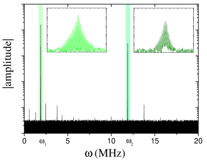
Figure 3: (Color online) Spectrum of the engaged cantilever motion with two flexural modes. Two highest peaks are clearly seen above noise level near resonant frequencies $\omega_{1}$ and $\omega_{2}$ which consist of the intermodulation products depicted in insertions. The spectrum is obtained by integrating the system (16) with the tip-surface force (22) and consequent addition of a white noise.

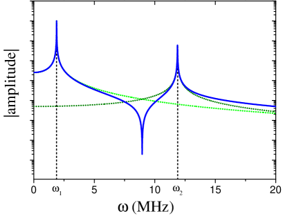
Figure 4: (Color online) Total transfer function $\chi$ (blue solid line) for the cantilever with two flexural modes with transfer functions $\chi_{1}$ and $\chi_{2}$ (light and dark green dotted lines respectively).

Prior to force reconstruction it is necessary to investigate what kind of information about $F_{z}$ is contained in the spectral bands for $z_{1}$ and $z_{2}$. In the current investigation we try to reconstruct the force using information contained only in the narrow frequency bands near $\omega_{1}$ and $\omega_{2}$, so all weak response peaks outside these bands are discarded. We also require that the second resonance frequency $\omega_{2}$ is not an integer multiplier of the $\omega_{1}$, so the second band does not capture any higher harmonics and intermodulation products produced by the drive in the first band. If $\omega_{2}$ were a harmonic of $\omega_{1}$ it would be of considerable advantage for force measurement Sahin et al. (2004). Considering the monomial basis (18) we can approximately evaluate the Fourier spectrum of the $i^{\mathrm{th}}$ power $\mathcal{F}[z^{k}]=\mathcal{F}[z]\ast\dots\ast\mathcal{F}[z]$ via convolution of the transfer function $\chi$ with itself, which gives an upper bound of the response in the frequency domain. Figure 5(a) demonstrates that only components with odd powers $i$ have significant value in the narrow bands near the resonances. Consequentially, only parameters $g_{i}$ for odd powers $z^{i}$ ($i$ odd) can be found directly using the measured spectrum.

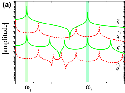
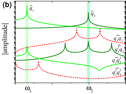
Figure 5: (Color online) (a) Response spectra for powers of single dynamic variable with two resonances and (b) two separate variables with one resonance. Two frequency windows near resonances $\omega_{1}$ and $\omega_{2}$ are highlighted with light and dark green colors respectively. Red dashed line means that the corresponding maximum response lies outside the frequency bands.

Having solved the system for the odd parameters, we can use them to recover the even parameters by applying an additional constraint: that the tip-surface force for tip positions above its rest point equals zero $F_{z}(z>0)=0$ which leads to the system

$$\sum\limits_{i=0}^{N/2}g_{2i}z_{k}^{2i}=\sum\limits_{i=0}^{N/2}g_{2i+1}z_{k}^{2i+1}$$ (20)

for all $z_{k}>0$ measured at discrete time moments $t_{k}$.

Reconstruction of the velocity-dependent part of $F_{z}$ is achieved by adding a new variable $\dot{z}=\dot{z}_{1}+\dot{z}_{2}$ to the model (18) which consequently increases the number of parameters by the degree of the polynomial in $\dot{z}$

$$\tilde{F}_{z}(z,\dot{z})=\sum\limits_{i=0}^{P_{z}}\sum\limits_{j=0}^{P_{\dot{z}}}g_{ij}z^{i}\dot{z}^{j}$$ (21)

Noticing that $\mathcal{F}[z^{i}\dot{z}^{j}]\propto\mathcal{F}[z^{i+j}]$, only coefficients $g_{ij}$ in front of $z^{i}\dot{z}^{j}$ where $i+j$ is odd can be determined from the measured spectrum. While coefficients before $z\dot{z}$, $z^{3}\dot{z}$, $z\dot{z}^{3}$, etc. can be found using the system (20).

We simulate the collinear bimodal case using the CVODE integrator Hindmarsh et al. (2005) with: $\omega_{1}=2\pi\,300$ kHz, $k_{1}=40$ N/m, $Q_{1}=400$, $\omega_{2}=6.3\omega_{1}$, $k_{2}=50k_{1}$, $Q_{2}=3Q_{1}$ (ratios for the second mode are taken from Lozano et al. (2010)). The driving forces $\mathrm{f}_{1,2}$ are chosen to have the same phase and give equal maximum free response (when $F_{z}\equiv 0$) at each mode $A_{z_{1}}=A_{z_{2}}=12.5$ nm so the total maximum amplitude of oscillations is $A_{z}=25$ nm; all four drive frequencies $\omega_{1,2}\pm\delta\omega/2$ are integer multipliers of base frequency $\delta\omega=2\pi\,0.2$ kHz. The engaged height $h$ above the surface is $17$ nm. The model of the tip-surface force $F_{z}$ is the vdW-DMT force Derjaguin et al. (1975) with the nonlinear damping term exponentially dependent on the tip position

$$\begin{array}[]{lcl}F_{z}(z,\dot{z})=F_{z}^{con}(z)+F_{z}^{dis}(z,\dot{z})\\ F_{z}^{con}(z)=\begin{cases}-\frac{HR}{6z^{2}},&z\geq a_{0}\\ -\frac{HR}{6a_{0}^{2}}+\frac{4}{3}E^{*}\sqrt{R(a_{0}-z)},&z<a_{0}\end{cases}\\ F_{z}^{dis}(z,\dot{z})=-\left(\gamma_{1}\dot{z}+\gamma_{3}\dot{z}^{3}\right)e^{-z/\lambda_{z}}\end{array}$$ (22)

with the following seven phenomenological parameters: intermolecular distance $a_{0}=0.3$ nm, Hamaker constant $H=7.1\times 10^{-20}$ J, effective modulus $E^{*}=1.0$ GPa, tip radius $R=10$ nm, damping decay length $\lambda_{z}=1.5$ nm, damping factors $\gamma_{1}=2.2\times 10^{-7}$ kg/s and $\gamma_{3}=10^{-22}$ kg$\cdot$s/m² (fig. 6(a)).

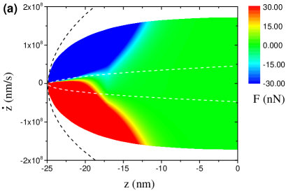
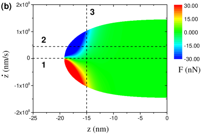
Figure 6: (Color online) (a) vdW-DMT force with position dependent damping in the region of the free tip motion with bimodal drive. White and black dashed lines confine covered domains of phase space in case of single mode drive of the first and second modes respectively (difference between maximum velocities is about order of magnitude). In all three cases, total maximum amplitude of oscillations is kept constant and equals $25$ nm. (b) Reconstructed force in the region of the engaged tip motion. Its cross-sections 1–3 are depicted in fig. 7(a)–(c) to highlight agreement between the actual force used in simulation and the reconstructed force.

It is worth noting that the calibration of the higher eigenmodes parameters $\omega_{i}$, $Q_{i}$ and $k_{i}$ which is required for force reconstruction, is itself a challenging task in multimodal AFM Lozano et al. (2010); Green et al. (2004); Feiler et al. (2000).

Using $B_{1,2}=24$ peaks in each band (fig. 3) for the reconstruction, we assume the model (21) degree in $z$ to be $P_{z}=21$. Numerical results show that the force reconstruction using higher powers of $\dot{z}^{i}$ ($i>1$) is less reliable as it encounters difficulties connected with multivariate interpolation. Although two modes give us twice the number of spectral components in comparison with singlemode case, this additional information is still insufficient for reconstruction of nonlinear (non-viscous) damping. Therefore, we are restricted the model to be linear in $\dot{z}$.

This numerical analysis suggests that there is no difference in the quality of the reconstructed force using intermodulation products from frequency bands surrounding the first, second or both resonances. We show results for the reconstructed $\tilde{F}_{z}(z,\dot{z})$ and its cross-sections in fig. 6(b) and fig. 7 using only the resonant detection band around the first eigenmode.

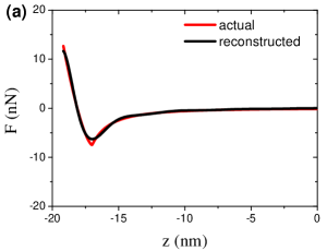
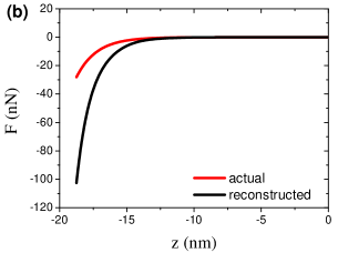
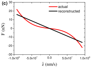
Figure 7: (Color online) Cross-sections of the reconstructed tip-surface force (black) with comparison to the actual force used in simulation (red) for the cantilever driven at two flexural modes. (a) $\tilde{F}_{z}(z,\dot{z}=0)$; (b) $\tilde{F}_{z}(z,\dot{z}=0.2\dot{z}_{\max})-\tilde{F}_{z}(z,\dot{z}=0)$; (c) $\tilde{F}_{z}(z=0.75z_{\min},\dot{z})$. Linear fit for nonlinear damping catches nicely overall trend and conservative part demonstrates an excellent agreement with the actual force.

The linear fit (21) for the model with nonlinear damping (22) nicely captures the overall trend of the dissipative part and the reconstructed conservative part demonstrates excellent agreement with the actual force. If we simulate the system (16) using the force $F_{z}$ linear in $\dot{z}$, for instance assuming $\gamma_{3}=0$ in (22), the reconstructed force $\tilde{F}_{z}$ shows nearly perfect agreement with the actual force $F_{z}$ (figures are not included).

One can compare the information contained in the two frequency bands near each eigenmode resonance by estimating the quality of the reconstruction as a function of the number of spectral components $B_{1,2}$ used in the reconstruction, as the least square error function

$$e_{i}(B_{i})=\int\limits_{z_{\min}}^{z_{\max}}\left[\tilde{F}_{z}(z,\dot{z}|B_{i})-F_{z}(z,\dot{z})\right]^{2}\mathrm{d}z$$ (23)

This error function plotted versus the number of spectral components is depicted in fig. 8.

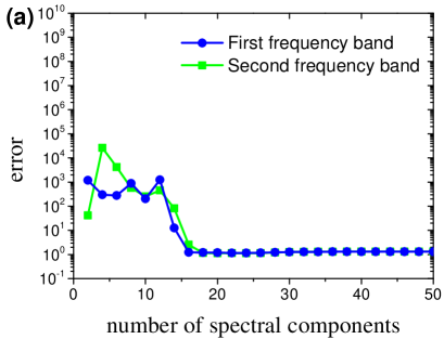
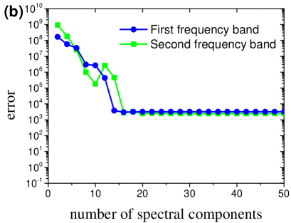
Figure 8: (Color online) Absolute error of reconstruction of (a) conservative part of the tip-surface force (fig. 7(a)) and (b) dissipative part (fig. 7(b)) versus number of spectral components taken into account in the first frequency band (blue circles) and in the second (green squares).

We see similar behavior for both bands: significant drop for the number of spectral components lager than half of the polynomial power $P_{z}=21$ in the expansion of $\tilde{F}_{z}$, and no qualitative improvements after reaching a number of spectral components less than $P_{z}$.

Another interesting observation regards the reconstruction of a dissipative force which turns-on only for the tip velocities $\dot{z}$, higher than the maximum velocity of the first mode $z_{1}$ (for some constant amplitude) and is zero otherwise. Information from both bands gives approximately the same reconstructed curves with showing overall trend of the dissipative part and in excellent agreement for the conservative part (plots not shown). However, reconstructing with spectral components from only the first frequency band yields more accurate dissipative force approximation as $z_{1}$ has smaller stored oscillation energy and, consequently, is more vulnerable to the dissipative force than $z_{2}$. Nonetheless, if we excite only the first mode, we would not be able to reconstruct this ”threshold” dissipative force at all, as the magnitude of the tip velocity would not be enough to turn on the dissipation. Thus, simultaneous excitation of two eigenmodes allows to explore a wider region of the phase space of the tip motion (fig. 6(a)) while keeping the total maximum amplitude constant.

IV.2 Case 2: Two orthogonal modes

This case corresponds to the dynamics of one flexural $z$ and one torsional $y$ mode

$$\begin{array}[]{lcl}k_{z}\left(\frac{1}{\omega_{z}^{2}}\ddot{z}+\frac{1}{Q_{z}\omega_{z}}\dot{z}+z\right)=F_{z}(z,y)+\mathrm{f}_{z}(t)\\ k_{y}\left(\frac{1}{\omega_{y}^{2}}\ddot{y}+\frac{1}{Q_{y}\omega_{y}}\dot{y}+y\right)=F_{y}(z,y)+\mathrm{f}_{y}(t)\end{array}$$ (24)

with two different projections of the conservative force, $F_{z}$ and $F_{y}$ on the r.h.s.

We start from the polynomial models for reconstruction

$$\begin{array}[]{lcl}\tilde{F}_{z}(z,y)=\sum\limits_{i=0}^{P_{z}}\sum\limits_{j=0}^{P_{y}}g^{(z)}_{ij}z^{i}y^{j}\\ \tilde{F}_{y}(z,y)=\sum\limits_{i=0}^{P_{z}}\sum\limits_{j=0}^{P_{y}}g^{(y)}_{ij}z^{i}y^{j}\end{array}$$ (25)

As for case 1 it is not possible to find all parameters of these models. Firstly, as we are limited in number of measurable intermodulation products and therefore in maximum degree of the polynomial. We choose $z$ direction as the most interesting degree of freedom, by which we mean that the maximum degree of the polynomial in this variable will be much higher than for $y$. In accordance to the fig. 5(b), the captured information about forces $\tilde{F}_{z}$ will be odd in $z$ and even in $y$ and vice versa for $\tilde{F}_{y}$

$$\begin{array}[]{lcl}\tilde{F}_{z}(-z,\pm y)=-\tilde{F}_{z}(z,y)\\ \tilde{F}_{y}(\pm z,-y)=-\tilde{F}_{y}(z,y)\end{array}$$ (26)

as the first flexural resonance $\omega_{z}$ is typically far lower in frequency than the first torsional resonance $\omega_{y}$ Raman et al. (2008). It is possible to recover the coefficients $g^{(z)}_{ij}$ of even powers of $y$ and $g^{(y)}_{ij}$ of odd powers of $y$ (when $i+j$ is even) by using the additional constraint for $z$ dependence of the force components $F_{z,y}(z>0,y)=0$ and eq. (20). While the information about all coefficients of $\tilde{F}_{z}$ with odd powers of $y$ and $\tilde{F}_{y}$ with even powers of $y$ is lost because we have no such constraint on the $y$ dependence.

Simulation parameters for the system (24) are: $\omega_{z}=2\pi\,300$ kHz, $k_{z}=40$ N/m, $Q_{z}=400$, $\omega_{y}=6.3\omega_{y}$, $k_{y}=50k_{y}$, $Q_{2}=3Q_{y}$. The driving forces $\mathrm{f}_{z,y}$ are chosen to have the same phase and give maximum free response (when $F_{z,y}\equiv 0$) $A_{z}=25$ nm and $A_{y}=12.5$ nm; all four drive frequencies $\omega_{z,y}\pm\delta\omega/2$ are integer multipliers of base frequency $\delta\omega=2\pi\,0.2$ kHz. The engaged height $h$ above the surface is $17$ nm. The model for the component of the tip-surface force perpendicular to the surface is the same vdW-DMT force (22) used in the previous case, without the dissipation term $F_{z}^{dis}$. The model of the force component parallel to the surface is a nonlinear conservative restoring force

$$F_{y}(z,y)=-\left(c_{1}y+c_{3}y^{3}\right)e^{-z/\lambda_{z}}$$ (27)

where $\lambda_{z}=1.5$ nm, $c_{1}=0.22$ N/m and $c_{3}=0.1$ N/m³ are constants. These two components of $\mathbf{F}_{ts}(\mathbf{r})$ are illustrated in fig. 9(a)–(b).

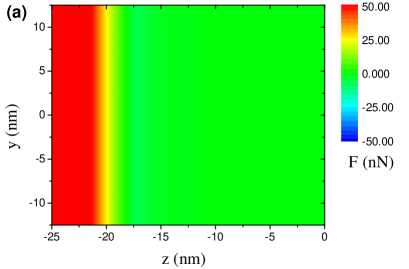
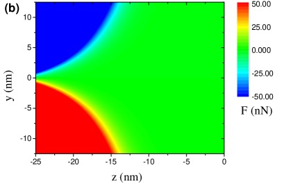
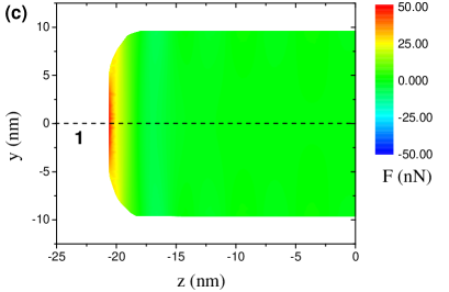
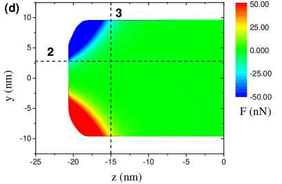
Figure 9: (Color online) Components $F_{z}$ and $F_{y}$ of two-dimensional conservative force in the region of the free tip motion (a,b) and reconstructed components in the region of the engaged tip motion (c,d). Cross-sections 1–3 are illustrated in fig. 10(a)–(c) to highlight agreement between the actual force used in simulation and the reconstructed force.

Using only $24$ intermodulation peaks in each band for $\hat{z}$ and $\hat{y}$, the spectral fitting method reconstructs the two-dimensional vector force field $\mathbf{F}_{ts}$ (22) and (27) up to the $21^{st}$ power in $z$ and third power in $y$ (fig. 9(c)–(d) and 10).

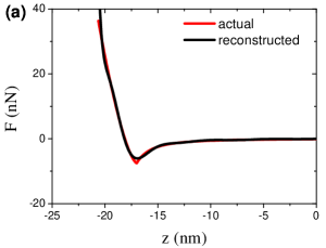
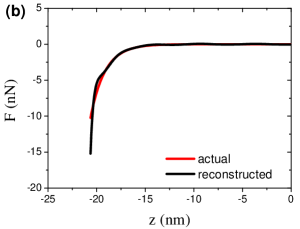
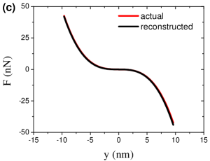
Figure 10: (Color online) Cross-sections of reconstructed tip-surface force (black) with comparison to the actual force used in simulation (red) for the cantilever driven at two orthogonal modes. (a) $\tilde{F}_{z}(z)$; (b) $\tilde{F}_{y}(z,y=0.2\dot{z}_{\max})$; (c) $\tilde{F}_{y}(z=0.75z_{\min},y)$. Reconstructed force is in a good agreement with underlying model. Perfect agreement is reachable if we assume model for $F_{z}$ independent of $y$.

The reconstructed force is in good agreement with the actual model and perfect agreement is reachable if we assume the model for $\tilde{F}_{z}$ as eq. (25) only, independent of $y$.

V Concluding remarks

In this paper we have discussed the basic problem of multimodal ImAFM and we proposed a theoretical framework for reconstructing multidimensional forces using this technique. We demonstrated the possibility of reconstructing tip-surface interactions for two characteristic bimodal cases. We have studied tip-surface interactions that show the most nonlinear behavior in the first degree of freedom, and are linear or cubic in the second degree of freedom. As the numerical results have shown, it is possible to accurately reconstruct dependencies up to a cubic order in the second degree of freedom for the two-dimensional force model using information from only one frequency band. We found that excitation of two flexural modes with two well separated resonances does not allow for a precise reconstruction of a nonlinear damping force using only the information contained in corresponding narrow bands near the resonances. However, the reconstruction nicely captures the overall linear trend, or that of a viscous damping. The use of a second, higher frequency eigenmode allows for reconstruction on a wider region of the phase space of a tip motion, enabling exploration of dissipative interactions inaccessible to the first mode alone for a given maximum amplitude of motion. Additionally, the first eigenmode is found to be more sensitive to dissipation forces acting on the tip. Finally, using simultaneous excitation of two orthogonal modes we can reconstruct nonlinear position-dependent lateral forces simultaneously with vertical forces. This approach represents a path toward the determination of a vectorial force field by frequency domain multiplexing of the multimodal response of an AFM cantilever.

*

Appendix A Generalized eigencoordinates

We start from the governing equation for a two-dimensional cantilever

$$\left(\mathcal{G}_{xy}+\mathcal{G}_{t}\right)\left[w\left(x,y,t\right)\right]=F(x,y,t)$$ (28)

and try to find solution $w\left(x,y,t\right)$ separated in time and space, and expanded into the set of normal modes

$$w(x,y,t)=\sum\limits_{i=0}^{\infty}\phi_{i}(x,y)q_{i}(t)$$ (29)

Functions $\phi_{i}$ form orthonormal set on the geometrical shape of cantilever $\Omega_{c}$

$$\int\limits_{\Omega_{c}}\phi_{i}\phi_{j}\,\mathrm{d}\Omega_{xy}=\delta_{i}^{j}$$ (30)

where $\delta_{i}^{j}$ is Kronecker delta equals $1$ for $i=j$ and $0$ otherwise.

Inserting solution (29) into eq. (28) with following multiplication by $\phi_{i}$ and integrating over the plane $\Omega_{c}$ yields a system of differential equations for the generalized coordinates $q_{i}(t)$

$$q_{i}\int\limits_{\Omega_{c}}\phi_{i}\mathcal{G}_{xy}\phi_{i}\,\mathrm{d}\Omega_{xy}+\mathcal{G}_{t}[q_{i}]\int\limits_{\Omega_{c}}\phi_{i}^{2}\,\mathrm{d}\Omega_{xy}=\int\limits_{\Omega_{c}}F(\Omega,t)\phi_{ij}\,\mathrm{d}\Omega_{xy}$$ (31)

here the orthonormal condition (30) is used.

Denoting $\mathcal{G}_{i}$ as a differential operator governing motion of $i^{\mathrm{th}}$ generalized coordinate

$$\mathcal{G}_{i}=k_{i}+m_{i}\mathcal{G}_{t}$$ (32)

where

$$\begin{array}[]{lcl}k_{i}\equiv\int\limits_{\Omega_{c}}\phi_{i}\mathcal{G}_{xy}\phi_{i}\,\mathrm{d}\Omega_{xy}\\ m_{i}\equiv\int\limits_{\Omega_{c}}\phi_{i}^{2}\,\mathrm{d}\Omega_{xy}\end{array}$$ (33)

are effective stiffness and mass of corresponding degree of freedom, and considering damping and inertia

$$\mathcal{G}_{t}:=\frac{\partial^{2}}{\partial t^{2}}+\gamma\frac{\partial}{\partial t}$$ (34)

with some constant $\gamma$ (homogeneous viscous medium damping), we arrive at the final system

$$k_{i}\left(\frac{1}{\omega_{i}^{2}}\ddot{q}_{i}+\frac{1}{Q_{i}\omega_{i}}\dot{q}_{i}+q_{i}\right)=F_{i}\left(t\right)+\mathrm{f}_{i}\left(t\right)$$ (35)

where resonant frequencies $\omega_{j}=\sqrt{k_{i}/m_{i}}$ and quality factors $Q_{i}=\omega_{i}/\gamma$ are introduced. Here the time-dependent forces

$$F_{i}\left(t\right)+\mathrm{f}_{i}\left(t\right):=\int\limits_{\Omega_{c}}\phi_{i}(x,y)F(x,y,t)\,\mathrm{d}\Omega_{xy}$$ (36)

represent anharmonic contribution of the tip-surface interaction and harmonic contribution of the drive, respectively.