Demonstration of Free-space Reference Frame Independent Quantum Key Distribution

Abstract

Quantum key distribution (QKD) is moving from research laboratories towards applications. As computing becomes more mobile, cashless as well as cardless payment solutions are introduced, and a need arises for incorporating QKD in a mobile device. Handheld devices present a particular challenge as the orientation and the phase of a qubit will depend on device motion. This problem is addressed by the reference frame independent (RFI) QKD scheme. The scheme tolerates an unknown phase between logical states that varies slowly compared to the rate of particle repetition. Here we experimentally demonstrate the feasibility of RFI QKD over a free-space link in a prepare and measure scheme using polarisation encoding. We extend the security analysis of the RFI QKD scheme to be able to deal with uncalibrated devices and a finite number of measurements. Together these advances are an important step towards mass production of handheld QKD devices.

1 Introduction

Quantum key distribution promises secure communications based not on the hardness of a mathematical problem but on the laws of physics [1, 2, 3]. The main effort in the development of QKD is directed towards long range communication, mostly fibre-based [4, 5, 6, 7, 8, 9] as well as in free space [10, 11, 12, 13]. A prospective new application of QKD is in securing short range line of sight communications between a terminal and a handheld device (see Fig 1a) [14, 15]. Current mobile payment techniques, e.g. Near Field Communications, have a range of security challenges including eavesdropping. Similar considerations apply to securing Wi-Fi access points. We believe that future handheld QKD systems can address these security challenges and provide a high degree of wireless security.

One of the unique problems faced by handheld QKD is the fact that the relative orientation of the emitter and the receiver is variable. In previous works this problem has been addressed by using entanglement [16] or by encoding information on angular momenta [17], which are invariant under rotation. The Reference Frame Independent QKD scheme proposed in [18] does not require entanglement and allows the use of polarisation encoding without the need for alignment of the qubit reference frames. In this scheme the qubits are prepared and measured in three mutually unbiased bases. Only one of those bases, on which the key is encrypted, needs to be stable. The two other bases are allowed to drift slowly and are used to estimate the security parameters of the quantum channels. The requirement for one basis to be stable is met in most practical implementations. In the case of free-space polarisation-based encoding, the stable basis is the circular polarisation, which is rotation independent. Fig 1b shows the bases used by the emitter (Alice) $X_{A}$, $Y_{A}$, $Z_{A}$ and the receiver (Bob) $X_{B}$, $Y_{B}$, $Z_{B}$ for an undetermined relative orientation. The use of additional bases compared to e.g. BB84 enables the reference frame independence of the scheme.

In order to demonstrate the feasibility of such a protocol we implement a prepare and measure scheme based on faint pulses and analyse the security of the channel. In addition to the reference frame independence implied by the protocol, we develop a theoretical analysis that allows us to take into account deviations from the ideal perpendicular preparation and measurement bases. This is similar in spirit to device independent QKD (e.g. [19]). Although we cannot claim to achieve full device independence, which generally requires entanglement, we are able to deal with device imperfections and uncalibrated devices within our selected model. In any QKD scheme the number of measurements available for the parameter estimation step is finite. Parameters obtained from the measurements are estimates with a non-zero variance, which impacts the secure key fraction as discussed in [20, 21, 22]. In our security analysis we take this into account to derive a secret key fraction. In this article, section 2 describes the experimental setup we used to implement a RFI protocol, while in section 3 we analyse the security of the quantum channel including the influence of finite size effects, imperfectly calibrated devices and mismatched detector efficiencies. In section 4 we discuss our results.

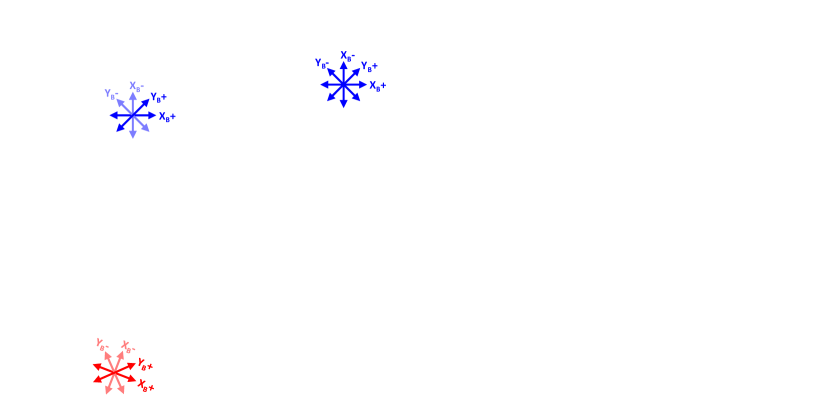
Figure 1: a) A mobile QKD terminal communicating with a stationary QKD terminal. The mobile terminal is free to rotate. b) Poincaré sphere representation of Alice and Bob’s reference frames. The Z basis (circular polarisation), represented by black vectors, is shared by Alice and Bob and is used as the key basis. Alice’s X and Y bases (horizontal/vertical and diagonal/antidiagonal), represented by red vectors, are aligned with the Poincaré sphere’s axes. Bob’s X and Y bases, represented in blue, are rotated with respect to Alice’s. A rotation of the terminal by the angle $\phi$ results in a rotation on the Poincaré sphere by $2\phi$.

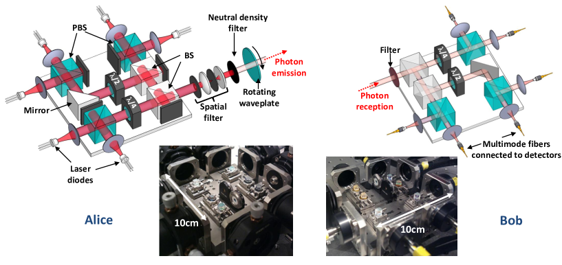
Figure 2: Experimental implementation of RFI QKD with the layout of the emitter (Alice’s device) and the receiver (Bob’s device). On Alice’s side, unpolarised light is produced by six laser diodes directed towards the two inputs of three polarising beam splitters. The outputs of the polarising beam splitters are polarised either horizontally or vertically depending on which laser is active. One of the outputs passes through a $22.5\textdegree$ rotated $\lambda/2$ waveplate resulting in diagonal/antidiagonal polarisations. Another PBS output is directed towards a $45\textdegree$ rotated $\lambda/4$ waveplate resulting in left/right circular polarisations. The last polarising beam splitter output’s polarisation is left unchanged. The three resulting beams are combined with two non-polarising beam splitters. The spatial profile of the combined beams is filtered with a $1\,\textnormal{mm}$ pinhole, while the direction profiles are filtered with a $5\,\mu\textnormal{m}$ pinhole between two lenses. Finally, light passes through a spectral filter and a neutral density filter reducing the intensity to single photon level. After the output of the emitter, a rotating $\lambda/2$ waveplate is used to simulate a rotation between the emitter and the receiver. The optical arrangement of the receiver is similar to the emitter except that optical fibres leading to the detectors are mounted instead of the lasers. Both Alice and Bob’s device are mounted on a $10\,\textnormal{cm}$ by $10\,\textnormal{cm}$ metal plate and the distance between the two is slightly above $1\,\textnormal{m}$. The compactness of our assembly can be seen in the insets.

2 Experimental setup

In the prepare and measure RFI protocol, Alice needs to be able to randomly pick a light polarisation state out of three different bases, i.e. horizontal/vertical, antidiagonal/diagonal, left circular/right circular, corresponding to X, Y and Z basis. This is implemented by activating one of six 850 nm VCSEL laser diodes. Their respective polarisations are separately engineered before their optical beams are combined in a common mode. They are electrically driven by a pattern generator with six individually controllable outputs. Each output generates 0.5 ns pulses and their amplitudes are adjusted so that the average photon number per pulse at Alice’s output is the same for all the lasers. Random bit sequences allowing only one of the six lasers to be active every 4 ns (i.e., $250\times 10^{6}$ pulses per second) are programmed in the pattern generator’s memory. Engineering of the polarisations is performed by a set of polarising beam splitters (PBS), and waveplates (see Fig 2). At first the polarisation of the VCSELs is ill-defined but it is filtered by the polarisation beam splitters with an extinction ratio of about 13 dB. The outputs of the polarising beam splitters are polarised either horizontally or vertically depending on which laser is active. One of the PBS output’s polarisation is left unchanged. The output of another PBS passes through a $22.5\textdegree$ rotated $\lambda/2$ waveplate resulting in diagonal/antidiagonal polarisations. The output of the last PBS is directed towards a $45\textdegree$ rotated $\lambda/4$ waveplate resulting in left/right circular polarisations. The waveplate used in this experiment are achromatic but we estimate their retardance at $850\,\textnormal{nm}$ to be 0.535 and 0.265 (+/-0.05) for the half and quarter waveplates respectively. Those discrepancies together with the PBS extinction ratio are responsible for the biasing of the bases that are discussed in the theoretical section. After preparing the polarisations the three resulting beams are combined with two non-polarising beam splitters. The spatial profile of the combined beams is filtered with a $1\,\textnormal{mm}$ pinhole, while the direction profiles are filtered with a $5\,\mu\textnormal{m}$ pinhole between two lenses. Finally, light passes through a neutral density filter reducing the intensity down to below 0.05 photons per pulse. After the output of the emitter, a rotating $\lambda/2$ waveplate is used to simulate a rotation between the emitter and the receiver. The photons then travel through free space for slightly more than a meter to the measurement terminal. At the input of the measurement device, a spectral filter with 10 nm passband and 0.7 maximum transmission is used to reduce background noise. The optical arrangement of the receiver is similar to the emitter except that it is used in reverse. The common optical mode is divided in three beams by the non-polarising beam splitters and waveplates are used before the PBSs to allow measurements in the three bases. Thus, the measurement basis is passively selected by the path of the photon, making it perfectly random. The six PBS outputs are coupled with approximately 0.8 efficiency to multimode optical fibres leading to single photon detectors. The photo detectors are silicon avalanche photodiodes with 0.45 efficiency at 850 nm, 400 dark counts per second, a timing resolution of 600 ps and 50 ns dead time. Their firing times as well as a clock pulse coming from the pattern generator are continuously recorded by a counting card. In post processing, we eliminate all the counts that happened when another detector was still in its dead time, i.e. whenever two counts happen within 60 ns. Bitrates could possibly be increased by using detection events in other detectors during a given detector’s deadtime, but the implications on security are unexplored. The remaining number of counts for a measurement duration of 1 s is approximately $2\times 10^{6}$ out of the $250\times 10^{6}$ weak pulses generated. The experiment is performed in the dark and owing to spectral filtering background noise is negligible compared to detector dark counts.

Finally, by matching recorded detection times with the original random patterns we can construct a 6 x 6 matrix (see Fig 3a) corresponding to the number of times one of the six detectors fired when one of the six lasers was active. The number of counts is maximal if the emitting and receiving polarisations are the same, it is minimal if they are opposite and it is approximately half of the maximum for all the other polarisations. This matrix constitutes the raw data of the security analysis. The counts in this matrix will be used for two different purposes. Half of the counts when both the sending and the measurement basis were Z are set aside as the raw key. The remaining half with all other counts forms the basis of the parameter estimation. The raw key length for each 1 s interval is approximately $2\times 10^{5}$. In order to demonstrate the robustness of our QKD scheme against reference frame rotations, we insert a half wave plate on a rotating mount in the free space optical path between the two terminals. Varying the optic axis angle of the half wave plate simulates rotations of Alice’s device. For each angle, a measurement is taken similar to that presented in Fig 3a. A comparison between measurement data and the 6 x 6 matrix predicted for ideal preparation and detection is shown in Fig 3b.

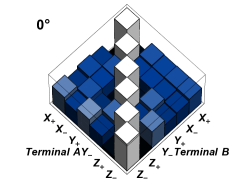
(a)

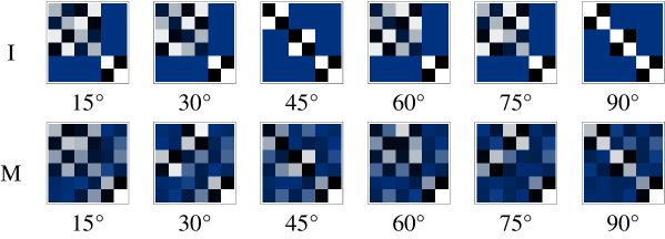
(b)

Figure 3: Results of the normalised detector count matrix for the implemented reference frame independent quantum key distribution protocol. Each matrix square represents the number of counts on the specified detector, when the specified polarisation was prepared. a) With the two reference frames aligned, corresponding preparation and measurement bases are almost completely correlated, with measurements between mutually unbiased bases showing almost no correlation. This indicates almost perfect transmission through the quantum channel. b) Comparison of ideal (I) and measured data (M) for six further reference frames, with angle of misalignment shown. While the counts contributing to the correlator $C_{ZZ}$ remain largely independent of the rotation angle, others contribute a periodic dependence to correlators $C_{XX}$, $C_{XY}$, $C_{YX}$ and $C_{YY}$. Counts contributing to the non-zero correlators $C_{XZ}$, $C_{YZ}$, $C_{ZX}$ and $C_{ZY}$ indicate that the X, Y and Z directions are not perpendicular.

The matching detector count patterns in Fig 3b already suggest that a quantum channel between the terminals is established, but in order to claim the possibility of quantum key distribution we need to analyse the results more rigorously.

3 Secure Key Fraction

The security of the RFI QKD protocol is discussed in [18]: Two parameters are estimated from the measurements: the quantum bit error rate $Q$ and a rotation invariant quantity $C$ (see B). While this analysis gives a good intuition why the scheme is reference frame independent, it does not take into account factors that can impact the key rate negatively in a real world setting, such as non-orthogonality of the measurement directions or finite size effects. In this section we derive the secure key fraction in the qubit subspace based on a model of the device including imperfect calibration of preparation and measurement bases, non uniform detector efficiencies and also the effect of a finite number of measurements. In general the calculation of the secret key fraction can be posed as an inference problem: given the measurements and a device model what is the maximum amount of information an eavesdropper can possess about the distributed key? We first introduce a simplified expression for the secure key fraction, then consider a model of our QKD system and minimise the secure key fraction subject to constraints derived from the model and the measurements.

The secure key fraction can be reduced from the ideal 100% due to leakage of information at two stages in the protocol [23]. During the quantum stage information can leak to an eavesdropper, while during error correction a certain minimum amount of information needs to be exchanged over a classical channel. The two terms of the following expression [24] for the secret key fraction reflect the impact of those two information leaks

$$r=S(\chi_{A}|\rho_{E})-H(\chi_{A}|\chi_{B}),$$ (1)

where $S(\cdot|\cdot)$ denotes the conditional von Neumann entropy, $H(\cdot|\cdot)$ the conditional Shannon entropy, $\chi_{A}$ are the classical bit values at terminal $A$, $\chi_{B}$ are the classical bit values at terminal $B$ and $\rho_{E}$ denotes the density matrix of the eavesdropper. The first term describes the entropy of the key bits $\chi_{A}$ given the eavesdropper’s information, we will call this “usable entropy”, $S_{U}$. The second term is the minimum necessary information to successfully perform error correction at the Shannon limit. In any real world implementation this number has to be multiplied by a factor larger than one to account for non-ideal error correction schemes. The main objective of the parameter estimation step is to find the minimum usable entropy given the constraints set by the measurements. These constraints also take into account the uncertainties associated with a finite number of performed measurements. Additionally the parameter estimation step provides information about the bit error rate, which is needed for error correction and thus an estimate for the second term. In our analysis we assume that the measurement results are produced by a two qubit density matrix $\rho_{AB}$ shared between parties $A$ and $B$. The usable entropy can be expressed as (see C)

$$S_{U}=S\left(\rho_{AB}||\mathcal{P}\rho_{AB}\right),$$ (2)

where $S\left(A||B\right)$ denotes the relative entropy and the super-operator $\mathcal{P}\rho=P_{0}^{A}\rho P_{0}^{A}+P_{1}^{A}\rho P_{1}^{A}$ with the projector on the bit values at terminal $A$ defined as $P_{0/1}^{A}=\frac{1}{2}\left(1\pm\sigma_{z}^{A}\right).$ To estimate the usable entropy we have to establish a model for our quantum key distribution system. This consists of a model of the quantum channel, embodied in the density matrix, along with a model of the terminal devices. The secret key fraction can be obtained as the minimum over all channel and device parameters that are consistent with the performed measurements. For a finite number of measurements the constraints will possess a statistical uncertainty that has to be taken into account in the minimisation procedure. As we are looking for an upper bound for the usable entropy it suffices to consider a simplified density matrix (see D), guaranteed to give a lower usable entropy than the full density matrix. The usable entropy for this density matrix becomes

$$S_{U}(\lambda_{1},\lambda_{2})=1+\sum_{i}\eta_{i}\log_{2}\eta_{i}-h\left(2\eta_{1}\right),$$ (3)

with the eigenvalues of the density matrix $\eta_{1}=\eta_{2}=1/4(1-\lambda_{1})$, $\eta_{3}=1/4(1+\lambda_{1}-2\lambda_{2})$ and $\eta_{4}=1/4(1+\lambda_{1}+2\lambda_{2})$ and $h(x)=-x\log_{2}x-(1-x)\log_{2}(1-x)$. With perfectly calibrated and aligned devices no additional model parameters have to be taken into account. Imperfect measurement devices can lead to a large number of additional parameters, such as non-orthogonalities in the preparation and measurement bases and detector efficiencies, which can be collected into the vector $\boldsymbol{\alpha}$ (for the details of the model see E). The usable entropy is obtained as the minimum over all parameters $\boldsymbol{\alpha}$, $\lambda_{1/2}$

$$S_{min}=\min_{\boldsymbol{\alpha},\lambda_{1},\lambda_{2}}S_{U}(\lambda_{1},\lambda_{2}).$$ (4)

The parameters have to obey the constraints imposed by the observations

$$f_{i}(\boldsymbol{m})-\sigma\delta f_{i}(\boldsymbol{m})\leq f_{i}\left[\boldsymbol{q}(\boldsymbol{\alpha},\lambda_{1},\lambda_{2})\right]\leq f_{i}(\boldsymbol{m})+\sigma\delta f_{i}(\boldsymbol{m}),$$ (5)

where $\boldsymbol{m}$ is a matrix containing all relevant detector counts, $\boldsymbol{q}$ is the corresponding probability of observing a detector count according to the device model (see E), the $f_{i}$ are the functions defining the different constraints, the $\delta f_{i}$ are their corresponding variances and $\sigma$ is chosen to give a certain probability that the estimated usable entropy is too high. In our parameter estimation step we use a set of 21 constraints (see F) consisting of 9 correlation functions $C_{AB},\,A,B=X,Y,Z$, the six probabilities that a photon was prepared in a certain polarisation direction $P_{A\pm},\,A=X,Y,Z$ and the six probabilities to detect in a certain detector $D_{B\pm},\,B=X,Y,Z$. For each function $f_{i}$ we can give the standard deviation $\delta f_{i}$ (see F). To obtain the secret key fraction we need to subtract the observed relative entropy in the key basis from the usable entropy

$$r=S_{min}-h\left(\frac{1-C_{ZZ}+\sigma\delta C_{ZZ}}{2}\right).$$ (6)

The full set of measurements enables us to calculate a reference frame independent key rate. From the detector counts we can construct 9 correlation functions

$$C_{AB}=\frac{m_{++}^{AB}+m_{--}^{AB}-m_{+-}^{AB}-m_{-+}^{AB}}{m_{++}^{AB}+m_{--}^{AB}+m_{+-}^{AB}+m_{-+}^{AB}},\,A,B=X,Y,Z,$$ (7)

where the $m_{\pm\pm}^{AB}$ are the four different detector counts given that the qubit was prepared in direction $A\pm$ and detected in direction $B\pm$. In the case of orthonormal preparation and measurement bases these can be directly identified with the qubit correlation functions. A secret key fraction can be obtained as the minimum key rate over all density matrices consistent with the observed correlators. In the BB84 protocol [25, 24] only two correlators, e.g. $C_{XX}$ and $C_{ZZ}$, are used as constraints. When the reference frames are rotated $C_{XX}$ will drop and so will the secret key fraction. The RFI QKD scheme uses the four correlators $C_{XX}$, $C_{XY}$, $C_{YX}$, $C_{YY}$ as well as $C_{ZZ}$. While each individual correlator may decrease under reference frame rotations, the combination $C=C_{XX}^{2}+C_{XY}^{2}+C_{YX}^{2}+C_{YY}^{2}$ ideally stays constant, enabling reference frame independent secret key fractions. In order to treat imperfect preparation and measurement we have to depart from the assumption of orthonormal bases and include a more detailed detector model. Each preparation and each detector are associated with a direction on the Poincaré sphere, given by a unit vector. Since we aim to use the z-basis for the key bits we can identify two preparation directions with the $\pm z$ direction on the Poincaré sphere, without overestimating the secret key fraction. Each direction is parametrised by two variables (e.g. azimuth and polar angle), resulting in a total of 20 free parameters (see E). Different absorption may occur in the preparation channels, and similarly detectors may have different efficiencies. With six possible preparation directions and six possible detection direction this adds another set of 12 parameters. The quantum channel can be represented by a two parameter two qubit density matrix in a simplification over the more commonly employed Bell diagonal density matrix (see D). This results in a model with 34 free parameters. The secret key fraction is then obtained as the minimum over all parameters that fulfil the constraints imposed by the measurements, e.g. from the correlators $C_{AB}$; in our case a set of 21 constraints. For the number of detector counts approaching infinity the constraints are equalities, but for a finite number of observations the value can lie within an interval determined by the number of counts and the desired uncertainty. A small number of counts will lead to larger uncertainty in the correlation function and therefore to lower results for the secret key fraction.

4 Results and Discussion

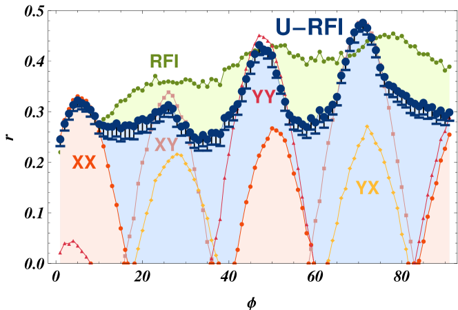
Figure 4: Keyrates as a function of the physical waveplate rotation angle for two reference frame independent and 4 different BB84 protocols. U-RFI labels the reference frame independent keyrate assuming uncalibrated devices. It is obtained from numerical minimisation over the full set of model parameters subject to constraints imposed by the measurements. The blue dots correspond to the minimised key rate neglecting the variance coming from the finite number of measurements. The blue bars indicate the result obtained by allowing for an uncertainty in the estimate of the constraints of three times the standard deviation. The remaining curves are obtained from the same data but with a simplified model, assuming orthogonality within bases and total perpendicularity between bases. RFI labels the keyrate for the reference frame independent protocol as outlined in [18]. XX, XY, YX and YY label the keyrates for the BB84 protocol using the respective correlator pairs $C_{ZZ}$ and $C_{XX}$, $C_{ZZ}$ and $C_{XY}$, and so on.

Our main result is that the secret key fraction remains above $0.2$ for all rotation angles even in the presence of device imperfections, see U-RFI in Fig 4. To better understand the calculated keyrate we make a comparison with established protocols: the BB84 protocol and the RFI QKD protocol as proposed by Laing, Scarani, Rarity and O’Brien [18]. For the sake of comparison we assume that in these protocols both preparation bases and measurement bases are perfect, i.e. the measured correlation functions are indeed the qubit correlation functions of the underlying density matrix. A summary of the calculation of the BB84 and RFI QKD key rates can be found in A and B. We clearly see in Fig 4 that while the BB84 key rate drops to zero for certain angles the RFI QKD key rate remains non-zero for all rotation angles. The plot also shows that for certain angles the RFI secret key fraction estimate is too optimistic compared to the U-RFI rates. This happens due to non-orthogonal measurement directions, which are not taken into account in the RFI QKD security analysis. The distinct peaks in the secret key fraction coincide with the peaks visible in the secret key fraction calculated for the BB84 protocols, as outlined above. This can be understood in the following way: The secret key fraction we calculate depends on the correlators $C_{AB},\,A,B=X,Y,Z$. The correlator $C_{ZZ}$ is linked to the qubit error rate. The correlators $C_{XX}$, $C_{XY}$, $C_{YX}$, $C_{YY}$ are related to monitoring the eavesdropping. If the absolute value of one of these correlators is large then eavesdropping in the key basis is small, even if other correlators are relatively small. This also makes the secret key fraction larger then the RFI keyrate for some angles. In the region between the peaks no individual correlator is large and only their combination gives a positive secret key fraction. In the presence of alignment errors some of the contributing correlators may be small and as a result the secret key fraction drops.

During each transmission of one second we set aside approximately $2\times 10^{5}$ raw key bits. After obtaining the correct secret key fraction from the parameter estimation step we can perform the privacy amplification step by applying the appropriate 2-universal hash function (e.g. a Toeplitz matrix [26]) to the raw key and obtain a secure key. With a secret key fraction of around $0.25$ we arrive at an approximate key rate of $5\times 10^{4}\,\textnormal{s}^{-1}$. In the current implementation of our scheme potential security loop holes exist due to side channels [27], the most obvious one coming from the use of six different lasers in the preparation stage. While this loophole can be plugged by using a single laser and a 1 x 6 optical switch further analysis of the impact of side channels on the key rate is required (e.g. the effect of photon number statistics [28] or detector characteristics [29] on our scheme).

Nevertheless we are able to give an estimate of the impact of photon number statistics on the key rate in our scheme. Without employing decoy states we have to assume that in pulses which contain more than one photon and which are contributing to the raw key all information is lost to the eavesdropper. Our photon source generates weak coherent pulses with a rate of $250\,\textnormal{MHz}$ and an average photon number of 0.05 per pulse. In order to assess the impact of a hypothetical photon number splitting attack we have to characterise the quantum channel. An important quantity is the accessible loss [30] in the quantum channel, i.e. the part of the loss that is, in principle, under the control of the eavesdropper. Due to the short range free space transmission no absorption occurs between Alice and Bob. A small amount of absorption (coupling efficiency$\approx 0.8$) can be attributed to the mode mismatch between sender and receiver and could be manipulated by an eavesdropper. All other losses occur in the Bob device and are inaccessible losses. Starting from a $250\,\textnormal{MHz}$ pulse rate and 0.05 photons per pulse we arrive at a raw single photon rate of $12.5\,\textnormal{MHz}$. The recorded photon count rate is $2\,\textnormal{MHz}$, giving a total absorption of $\eta$=0.16. The accessible part of the absorption is $\eta_{A}=0.8$, while the inaccessible part, containing absorption in filters, losses in optical components and finite detector efficiency contributes $\eta_{I}=0.2$, so that $\eta=\eta_{A}\eta_{I}$. The rate of two photon pulses according to Poisson statistics is $0.3\,\textnormal{MHz}$. The remaining single photons after a photon number splitting attack will still experience the inaccessible losses, so that the total number of recorded detector clicks associated with two photon pulses is $60\,\textnormal{kHz}$. Of these photons only a fraction contributes to the raw key. For our setup that fraction is $0.1$. For a key distribution lasting one second we estimate that an eavesdropper can at most have information about $6000$ key bits out of $2\times 10^{5}$ key bits, or the secure key fraction has to be reduced by approximately 0.03, due to the probabilistic nature of the photon source, only slightly modifying our secret key fraction.

In summary, we have shown the feasibility of reference frame independent key distribution using off the shelf bulk optical components in a compact assembly. Our setup uses passive components and can readily be transferred to a miniaturised version using integrated optics on a chip [31, 32]. Our analysis employed in the parameter estimation step obviates the need for precise alignment of the preparation and measurement qubit bases. The achievable key rates are sufficient to distribute hundreds of 256 bit keys within 1 second. In order to realise a handheld QKD device additional functionality, like steering of the emitted photons towards a receiver needs to be implemented. Possible solutions include movable mirrors, movable lenses or phased arrays. Overall, the work presented here paves the way for mass-produced handheld QKD devices.

Appendix A Keyrate for BB84

For the calculation of the keyrate for the BB84 protocol we follow [24], with the difference that we use two parameters for the quantum channel, the correlation functions $C_{XX}$ and $C_{ZZ}$ . The secure key fraction for the BB84 protocol is given by

$$r=\min_{\eta_{i}}\left(1+\sum_{i=1}^{4}\eta_{i}\log_{2}\eta_{i}\right)$$ (8)

under the constraints

$$C_{XX}=1-2\eta_{2}-2\eta_{4}$$ (9)

$$C_{ZZ}=1-2\eta_{3}-2\eta_{4}$$ (10)

$$\sum_{i=1}^{4}\eta_{i}=1.$$ (11)

This can be solved analytically to give

$$r=1+z_{+}x_{+}\log_{2}\left(z_{+}x_{+}\right)+z_{+}x_{-}\log_{2}\left(z_{+}x_{-}\right)+z_{-}x_{+}\log_{2}\left(z_{-}x_{+}\right)+z_{-}x_{-}\log_{2}\left(z_{-}x_{-}\right)$$ (12)

with

$$x_{\pm}=\frac{1\pm C_{XX}}{2},\quad z_{\pm}=\frac{1\pm C_{ZZ}}{2}$$ (13)

Alternatively other correlators than $C_{XX}$ can be used to obtain a keyrate. In the case of misaligned reference frames the correlators $C_{XY}$ or $C_{YX}$ may give a more favourable keyrate.

Appendix B RFI QKD

Reference frame independent quantum key distribution was introduced in [18]. The scheme solves the problem of aligning reference frames between two partners in a quantum key distribution protocol if one stable direction exists (e.g. in polarisation encoding physical rotation does not influence the circular polarisation direction). The stable direction is used for encoding the qubits, while perpendicular directions are used for parameter estimation. It is sufficient to consider two quantities constructed from the qubit correlation functions: the bit error rate

$$Q=\frac{1-C_{ZZ}}{2}$$ (14)

and the quantity

$$C=C_{XX}^{2}+C_{XY}^{2}+C_{YX}^{2}+C_{YY}^{2}.$$ (15)

with the qubit correlation functions given by

$$C_{AB}=\textnormal{Tr}\left(\sigma_{A}\sigma_{B}\rho\right),$$ (16)

where $\rho$ is the two qubit density matrix. Under rotations around the z axis the Pauli matrices transform $\sigma_{x}\rightarrow\sigma_{x}\cos\alpha+\sigma_{y}\sin\alpha$ and $\sigma_{y}\rightarrow\sigma_{y}\cos\alpha-\sigma_{x}\sin\alpha$, with the rotation angle given by $\alpha$. One can see that the quantity $C$ stays invariant under these kind of rotations. The secret key fraction can be shown to be a function of $C$ and $Q$. For $Q\lesssim 0.159$ the secret key fraction becomes

$$r=1-h(Q)-(1-Q)h\left(\frac{1+u}{2}\right)-Qh\left(\frac{1+v}{2}\right)$$ (17)

with $h(x)=-\log_{2}x-(1-x)\log_{2}(1-x)$ the Shannon entropy function and $u=\min(\sqrt{C/2}/(1-Q),1)$ and $v=\sqrt{C/2-(1-Q)^{2}u^{2}}/Q$.

Appendix C Conditional Entropy decreases under Projective Measurement

A quantum communication channel between parties Alice ($A$) and Bob ($B$) can be described by the density matrix $\rho_{AB}$. In general this density matrix will not be pure due to noise, errors and the action of an eavesdropper. In order to prove security of the communication channel we have to assume all deviations from the ideal case are due to an eavesdropper. The combined state of $\rho_{AB}$ and an eavesdropper can then be expressed as the pure state

$$|\psi>_{ABE}=\sum_{i=1}^{4}\sqrt{\lambda_{i}}|\Phi_{i}>_{AB}|\nu_{i}>_{E},$$ (18)

where the $\lambda_{i}$ are the eigenvalues of $\rho_{AB}$, $|\Phi_{i}>_{AB}$ are the corresponding eigenfunctions and $|\nu_{i}>$ are an orthogonal basis for the state of the eavesdropper. Note that the dimension of the Hilbert space of the eavesdropper equals the dimensions of $\rho_{AB}$. The density matrices in the subspaces can then be obtained as

$$\rho_{AB}=\textnormal{Tr}_{E}\left(|\psi>_{ABE}<\psi|_{ABE}\right)$$ (19)

and

$$\rho_{E}=\textnormal{Tr}_{AB}\left(|\psi>_{ABE}<\psi|_{ABE}\right).$$ (20)

The reduced density matrix of the eavesdropper equals the reduced density matrix of Alice and Bob up to a unitary transformation

$$\rho_{E}=U\rho_{AB}U^{\dagger}.$$ (21)

Let us consider the entropy of the key bits $\chi_{A}$ given that the eavesdropper knows the state of the system $\chi_{E}$, $S(\chi_{A}|\chi_{E})$. We can rewrite the conditional entropy as

$$S(\chi_{A}|\rho_{E})=S(\chi_{A})+S(\chi_{E}|\chi_{A})-S(\rho_{E}).$$ (22)

With $X$ being the classical value of Alice’s qubit we can write

$$S(\rho_{E}|\chi_{A})=\sum_{x=0,1}p_{x}S(E_{x})$$ (23)

If Alice prepares key bit 0 with probability $p_{0}$ and key bit one with probability $p_{1}$ we can write the corresponding density matrices $E_{0}$, $E_{1}$ with the help of the projection operators

$$P_{x}=|x>_{A}<x|_{A},\quad x=0,1$$ (24)

as

$$E_{x}=\textnormal{Tr}_{AB}\left(P_{x}|\psi>_{ABE}<\psi|_{ABE}\right)$$ (25)

or

$$E_{x}=\frac{1}{p_{x}}\sqrt{\rho_{AB}}P_{x}\sqrt{\rho_{AB}}.$$ (26)

Since unitary transformations do not change the entropy we can replace $\rho_{AB}$ with $\rho_{E}$ in the calculation of entropies

$$S\left(\frac{1}{p_{x}}\sqrt{\rho_{AB}}P_{x}\sqrt{\rho_{AB}}\right)=S\left(\frac{1}{p_{x}}\sqrt{\rho_{E}}P_{x}\sqrt{\rho_{E}}\right).$$ (27)

We can use

$$\textnormal{Tr}\left[\sqrt{\rho}P\sqrt{\rho}F(\sqrt{\rho}P\sqrt{\rho})\right]=\textnormal{Tr}\left[P\rho PF(P\rho P)\right],$$ (28)

where $F$ is any function and we used

$$F(\sqrt{\rho}P\sqrt{\rho})=\sum_{n}c_{n}(\sqrt{\rho}P\sqrt{\rho})=\sum_{n}\sqrt{\rho}P\left(P\rho P\right)^{n-1}P\sqrt{\rho}.$$ (29)

We can therefore write

$$S(\rho_{E}|\chi_{A})=\sum_{x=0,1}p_{x}S(\frac{1}{p_{x}}P_{x}\rho_{E}P_{x}).$$ (30)

Since the $P_{x}$ project onto orthogonal subspaces we can use (see Nielsen and Chuang, p.518 [33]) to write

$$S(\rho_{E}|\chi_{A})=S\left(\sum_{x=0,1}P_{x}\rho_{E}P_{x}\right)-S(\chi_{A}).$$ (31)

The equality holds if the projectors $P_{x}$ project onto orthogonal subspaces and acts as an upper bound on the usable entropy otherwise. The conditional entropy therefore becomes

$$S(\chi_{A}|\rho_{E})=S\left(\sum_{x=0,1}P_{x}\rho_{E}P_{x}\right)-S(\chi_{E}).$$ (32)

Introducing the projective measurement

$$\mathcal{P}\rho=\sum_{x}P_{x}\rho P_{x}$$ (33)

we can write

$$S(\chi_{A}|\rho_{E})=S\left(\mathcal{P}\rho_{E}\right)-S(\rho_{E}).$$ (34)

Since $\mathcal{P}$ is a projective measurement this simplifies further to the relative entropy

$$S(\chi_{A}|\rho_{E})=S\left(\rho_{E}||\mathcal{P}\rho_{E}\right)=S\left(\rho_{AB}||\mathcal{P}\rho_{AB}\right).$$ (35)

We now want to investigate how a further projective measurement influences the relative entropy. Introducing

$$\mathcal{L}\rho=\sum_{i}L_{i}\rho L_{i},$$ (36)

with the projection operators $L_{i}$. We consider the relative entropy before and after the projective measurement $\mathcal{L}$

$$S\left(\rho_{AB}||\mathcal{P}\rho_{AB}\right)-S\left(\mathcal{L}\rho_{AB}||\mathcal{P}\mathcal{L}\rho_{AB}\right).$$ (37)

For commuting operations

$$\mathcal{PL}=\mathcal{LP}$$ (38)

and using that the relative entropy of two density matrices decreases or stays the same under completely positive trace preserving maps [34] we obtain

$$S\left(\rho_{AB}||\mathcal{P}\rho_{AB}\right)-S\left(\mathcal{L}\rho_{AB}||\mathcal{L}\mathcal{P}\rho_{AB}\right)\geq 0$$ (39)

if the operations $\mathcal{L}$ and $\mathcal{P}$ commute.

Appendix D Simplified density matrices for parameter estimation

We can use the inequality above to simplify the model density matrix for parameter estimation. Starting from the full two qubit density matrix with 15 free parameters we can apply a series of projective measurements,

$$\mathcal{L}=\mathcal{L}_{2}\mathcal{L}_{1}$$ (40)

to arrive at a simpler density matrix with fewer parameters that is guaranteed to give a smaller value for the usable entropy. The individual projective measurement super-operators are

$$\mathcal{L}_{i}=\lim_{t\rightarrow\infty}e^{-t\mathcal{K}_{i}}$$ (41)

and the corresponding Liouvillian

$$\mathcal{K}_{i}\rho=\left\{\Sigma_{i}\Sigma_{i},\rho\right\}-2\Sigma_{i}\rho\Sigma_{i},\quad\Sigma_{1}=\sigma_{z}^{A}-\sigma_{z}^{B},\Sigma_{2}=\sigma_{x}^{A}\sigma_{x}^{B}.$$ (42)

If we use the z basis for the key bits then the measurement operator becomes

$$\mathcal{P}\rho=P_{0}^{A}\rho P_{0}^{A}+P_{1}^{A}\rho P_{1}^{A}$$ (43)

with the projector on the bit values at terminal $A$ defined as

$$P_{0/1}^{A}=\frac{1}{2}\left(1\pm\sigma_{z}^{A}\right)$$ (44)

It can be shown that

$$\mathcal{P}\mathcal{L}_{i}\rho-\mathcal{L}_{i}\mathcal{P}\rho=0$$ (45)

for all density matrices $\rho$. After applying all the projective measurements to a general density matrix the simplified density matrix takes the form

$$\rho=\frac{1}{4}\left(\begin{array}[]{cccc}1+\lambda_{1}&0&0&2\lambda_{2}\\ 0&1-\lambda_{1}&0&0\\ 0&0&1-\lambda_{1}&0\\ 2\lambda_{2}&0&0&1+\lambda_{1}\end{array}\right)$$ (46)

This density matrix can now be used in models for parameter estimation.

Appendix E Device model

We want to construct a model for the probability of registering a detector count in the detector measuring in basis $B$, direction $V$, provided the bit was prepared in basis $A$, direction $U$, $p_{UV}^{AB}$. The probability of observing a count in a detector given a certain preparation is proportional to

$$q_{UV}^{AB}=t_{AU}^{1}t_{BV}^{2}\textnormal{Tr}\left(\hat{P}_{AU}\hat{P}_{BV}\rho\right),$$ (47)

where $t^{1}$ and $t^{2}$ account for the preparation and detection efficiencies. The projectors $\hat{P}_{AU},\,\hat{P}_{BV}$ are along a certain preparation or measurement direction, given by a unit vector $\boldsymbol{n}_{AX}$ or $\boldsymbol{r}_{BY}$

$$\hat{P}_{AU}=\frac{1}{2}\left(1+\boldsymbol{n}_{AU}\cdot\boldsymbol{\sigma}_{A}\right),\quad\hat{P}_{BV}=\frac{1}{2}\left(1+\boldsymbol{r}_{BV}\cdot\boldsymbol{\sigma}_{B}\right),$$ (48)

where $\boldsymbol{\sigma}_{A/B}$ is a vector of Pauli matrices in the respective local basis. Using the simplified density matrix Eq. (46) we obtain

$$q_{UV}^{AB}=\frac{t_{AU}^{1}t_{BV}^{2}}{4}\left[1+\sum_{ij}n_{i}^{AU}r_{j}^{BV}\textnormal{Tr}\left(\hat{\sigma}_{i}^{A}\hat{\sigma}_{j}^{B}\rho\right)\right]$$ (49)

with

$$\textnormal{Tr}\left(\hat{\sigma}_{i}^{A}\hat{\sigma}_{j}^{B}\rho\right)=\delta_{ij}l_{i}=\Lambda_{ij},\quad\boldsymbol{l}=(\lambda_{2},\lambda_{2},\lambda_{1})$$ (50)

and therefore

$$q_{UV}^{AB}=\frac{t_{AU}^{1}t_{BV}^{2}}{4}\left(1+\boldsymbol{n}_{AU}\cdot\Lambda\cdot\boldsymbol{r}_{BV}\right).$$ (51)

so that the probabilities become

$$p_{UV}^{AB}=\frac{q_{UV}^{AB}}{\sum_{ABUV}q_{UV}^{AB}}.$$ (52)

For our measurement setup there are six distinct preparation directions $\boldsymbol{n}_{AU},\quad A=X,\,Y,\,Z,\quad U=\pm$, with two free parameters, the azimuthal and polar angle, specifying each direction. The z-direction is identified with the qubit directions at terminal A and therefore we fix $\boldsymbol{n}_{Z\pm}=(0,0,\pm 1)$. Similarly there are six measurement directions $\boldsymbol{r}_{BV},\quad B=X,\,Y,\,Z,\quad V=\pm$.

Appendix F Detector counts and correlation functions

The calculation of the secret key fraction is based on a minimisation subject to a number of constraints. In our implementation we use a total of 21 constraints. Each constraint and its corresponding standard deviation can be calculated from the raw detector counts obtained in the parameter estimation process. The first set of constraints is given by the 9 correlation functions

$$C_{AB}(\boldsymbol{m})=\frac{m_{++}^{AB}+m_{--}^{AB}-m_{+-}^{AB}-m_{-+}^{AB}}{m_{++}^{AB}+m_{--}^{AB}+m_{+-}^{AB}+m_{-+}^{AB}},\,A,B=X,Y,Z$$ (53)

Additional 6 constraints are the probabilities for preparing a certain direction

$$P_{AU}(\boldsymbol{m})=\frac{\sum_{BV}m_{UV}^{AB}}{N_{0}},\quad N_{0}=\sum_{ABUV}m_{UV}^{AB},$$ (54)

where $N_{0}$ is the total number of detector counts. Further 6 constraints are the probabilities for detecting a certain direction

$$D_{BV}(\boldsymbol{m})=\frac{\sum_{AU}m_{UV}^{AB}}{N_{0}}.$$ (55)

The corresponding standard deviations are

$$\delta C_{AB}(\boldsymbol{m})=\sqrt{\frac{4\left(m_{++}^{AB}+m_{--}^{AB}\right)\left(m_{+-}^{AB}+m_{-+}^{AB}\right)}{\left(m_{++}^{AB}+m_{--}^{AB}+m_{+-}^{AB}+m_{-+}^{AB}\right)^{3}}}.$$ (56)

and

$$\delta P_{AU}(\boldsymbol{m})=\sqrt{\frac{(N_{0}-\sum_{BV}m_{UV}^{AB})\sum_{BV}m_{UV}^{AB}}{N_{0}^{3}}},$$ (57)

as well as

$$\delta D_{BV}(\boldsymbol{m})=\sqrt{\frac{(N_{0}-\sum_{AU}m_{UV}^{AB})\sum_{AU}m_{UV}^{AB}}{N_{0}^{3}}}.$$ (58)

This gives us a total of 21 constraints derived from the raw detector counts to be used in the calculation of the secret key fraction.

References

- [1] N. Gisin, G. Ribordy, W. Tittel, and H. Zbinden. Quantum cryptography. Reviews of Modern Physics, 74:145–195, January 2002.
- [2] C. H. Bennett and G. Brassard. Int. conf. computers, systems & signal processing, bangalore, 1984.
- [3] A. K. Ekert. Quantum cryptography based on bell’s theorem. Phys. Rev. Lett., 67:661–663, 1991.
- [4] D. Stucki, M. Legré, F. Buntschu, B. Clausen, N. Felber, N. Gisin, L. Henzen, P. Junod, G. Litzistorf, P. Monbaron, L. Monat, J.-B. Page, D. Perroud, G. Ribordy, A. Rochas, S. Robyr, J. Tavares, R. Thew, P. Trinkler, S. Ventura, R. Voirol, N. Walenta, and H. Zbinden. Long-term performance of the SwissQuantum quantum key distribution network in a field environment. New Journal of Physics, 13(12):123001, December 2011.
- [5] M. Sasaki, M. Fujiwara, H. Ishizuka, W. Klaus, K. Wakui, M. Takeoka, S. Miki, T. Yamashita, Z. Wang, A. Tanaka, K. Yoshino, Y. Nambu, S. Takahashi, A. Tajima, A. Tomita, T. Domeki, T. Hasegawa, Y. Sakai, H. Kobayashi, T. Asai, K. Shimizu, T. Tokura, T. Tsurumaru, M. Matsui, T. Honjo, K. Tamaki, H. Takesue, Y. Tokura, J. F. Dynes, A. R. Dixon, A. W. Sharpe, Z. L. Yuan, A. J. Shields, S. Uchikoga, M. Legré, S. Robyr, P. Trinkler, L. Monat, J.-B. Page, G. Ribordy, A. Poppe, A. Allacher, O. Maurhart, T. Länger, M. Peev, and A. Zeilinger. Field test of quantum key distribution in the Tokyo QKD Network. Optics Express, 19:10387, May 2011.
- [6] M. Peev, C. Pacher, R. Alléaume, C. Barreiro, J. Bouda, W. Boxleitner, T. Debuisschert, E. Diamanti, M. Dianati, J. F. Dynes, S. Fasel, S. Fossier, M. Fürst, J.-D. Gautier, O. Gay, N. Gisin, P. Grangier, A. Happe, Y. Hasani, M. Hentschel, H. Hübel, G. Humer, T. Länger, M. Legré, R. Lieger, J. Lodewyck, T. Lorünser, N. Lütkenhaus, A. Marhold, T. Matyus, O. Maurhart, L. Monat, S. Nauerth, J.-B. Page, A. Poppe, E. Querasser, G. Ribordy, S. Robyr, L. Salvail, A. W. Sharpe, A. J. Shields, D. Stucki, M. Suda, C. Tamas, T. Themel, R. T. Thew, Y. Thoma, A. Treiber, P. Trinkler, R. Tualle-Brouri, F. Vannel, N. Walenta, H. Weier, H. Weinfurter, I. Wimberger, Z. L. Yuan, H. Zbinden, and A. Zeilinger. The SECOQC quantum key distribution network in Vienna. New Journal of Physics, 11(7):075001, July 2009.
- [7] A. R. Dixon, Z. L. Yuan, J. F. Dynes, A. W. Sharpe, and A. J. Shields. Continuous operation of high bit rate quantum key distribution. Applied Physics Letters, 96(16):161102, April 2010.
- [8] J. F. Dynes, H. Takesue, Z. L. Yuan, A. W. Sharpe, K. Harada, T. Honjo, H. Kamada, O. Tadanaga, Y. Nishida, M. Asobe, and A. J. Shields. Efficient entanglement distribution over 200 kilometers. Optics Express, 17:11440, June 2009.
- [9] A. Mirza and F. Petruccione. Recent Findings From The Quantum Network in Durban. In T. Ralph and P. K. Lam, editors, American Institute of Physics Conference Series, volume 1363 of American Institute of Physics Conference Series, pages 35–38, October 2011.
- [10] R. J. Hughes, J. E. Nordholt, D. Derkacs, and C. G. Peterson. Practical free-space quantum key distribution over 10 km in daylight and at night. New Journal of Physics, 4:43, July 2002.
- [11] R. Alléaume, F. Treussart, G. Messin, Y. Dumeige, J.-F. Roch, A. Beveratos, R. Brouri-Tualle, J.-P. Poizat, and P. Grangier. Experimental open-air quantum key distribution with a single-photon source. New Journal of Physics, 6:92, July 2004.
- [12] R. Ursin, F. Tiefenbacher, T. Schmitt-Manderbach, H. Weier, T. Scheidl, M. Lindenthal, B. Blauensteiner, T. Jennewein, J. Perdigues, P. Trojek, B. Ömer, M. Fürst, M. Meyenburg, J. Rarity, Z. Sodnik, C. Barbieri, H. Weinfurter, and A. Zeilinger. Entanglement-based quantum communication over 144km. Nature Physics, 3:481–486, July 2007.
- [13] T. Schmitt-Manderbach, H. Weier, M. Fürst, R. Ursin, F. Tiefenbacher, T. Scheidl, J. Perdigues, Z. Sodnik, C. Kurtsiefer, J. G. Rarity, A. Zeilinger, and H. Weinfurter. Experimental Demonstration of Free-Space Decoy-State Quantum Key Distribution over 144km. Physical Review Letters, 98(1):010504, January 2007.
- [14] M. S. Godfrey, A. M. Lynch, J. L. Duligall, W. J. Munro, K. J. Harrison, and J. G. Rarity. Free-space secure key exchange from 1 m to 1000 km. In Society of Photo-Optical Instrumentation Engineers (SPIE) Conference Series, volume 6399 of Society of Photo-Optical Instrumentation Engineers (SPIE) Conference Series, September 2006.
- [15] J. L. Duligall, M. S. Godfrey, K. A. Harrison, W. J. Munro, and J. G. Rarity. Low cost and compact quantum key distribution. New Journal of Physics, 8:249, October 2006.
- [16] J.-C. Boileau, R. Laflamme, M. Laforest, and C. R. Myers. Robust quantum communication using a polarization-entangled photon pair. Phys. Rev. Lett., 93:220501, Nov 2004.
- [17] V. D’Ambrosio, E. Nagali, S. P. Walborn, L. Aolita, S. Slussarenko, L. Marrucci, and F. Sciarrino. Complete experimental toolbox for alignment-free quantum communication. Nature Communications, 3, July 2012.
- [18] A. Laing, V. Scarani, J. G. Rarity, and J. L. O’Brien. Reference-frame-independent quantum key distribution. Physical Review A , 82(1):012304, July 2010.
- [19] Antonio Acin, Nicolas Brunner, Nicolas Gisin, Serge Massar, Stefano Pironio, and Valerio Scarani. Device-independent security of quantum cryptography against collective attacks. Phys. Rev. Lett., 98:230501, Jun 2007.
- [20] L. Sheridan, T. Phuc Le, and V. Scarani. Finite-key security against coherent attacks in quantum key distribution. New Journal of Physics, 12(12):123019, December 2010.
- [21] T. Meyer, H. Kampermann, M. Kleinmann, and D. Bruß. Finite key analysis for symmetric attacks in quantum key distribution. Physical Review A , 74(4):042340, October 2006.
- [22] V. Scarani and R. Renner. Quantum Cryptography with Finite Resources: Unconditional Security Bound for Discrete-Variable Protocols with One-Way Postprocessing. Physical Review Letters, 100(20):200501, May 2008.
- [23] V. Scarani, H. Bechmann-Pasquinucci, N. J. Cerf, M. Dušek, N. Lütkenhaus, and M. Peev. The security of practical quantum key distribution. Reviews of Modern Physics, 81:1301–1350, July 2009.
- [24] R. Renner, N. Gisin, and B. Kraus. Information-theoretic security proof for quantum-key-distribution protocols. Physical Review A , 72(1):012332, July 2005.
- [25] C. H. Bennett, G. Brassard, and N. D. Mermin. Quantum cryptography without Bell’s theorem. Physical Review Letters, 68:557–559, February 1992.
- [26] Hugo Krawczyk. New Hash Functions For Message Authentication. 1995.
- [27] S. Nauerth, M. Fürst, T. Schmitt-Manderbach, H. Weier, and H. Weinfurter. Information leakage via side channels in freespace BB84 quantum cryptography. New Journal of Physics, 11(6):065001, June 2009.
- [28] H.-K. Lo, X. Ma, and K. Chen. Decoy state quantum key distribution. Phys. Rev. Lett., 94:230504–, 2005.
- [29] N. Jain, C. Wittmann, L. Lydersen, C. Wiechers, D. Elser, C. Marquardt, V. Makarov, and G. Leuchs. Device Calibration Impacts Security of Quantum Key Distribution. Physical Review Letters, 107(11):110501, September 2011.
- [30] N. Lütkenhaus and M. Jahma. Quantum key distribution with realistic states: photon-number statistics in the photon-number splitting attack. New Journal of Physics, 4:44, July 2002.
- [31] A. Politi, M. J. Cryan, J. G. Rarity, S. Yu, and J. L. O’Brien. Silica-on-Silicon Waveguide Quantum Circuits. Science, 320:646–, May 2008.
- [32] J. L. O’Brien, A. Furusawa, and J. Vučković. Photonic quantum technologies. Nature Photonics, 3:687–695, December 2009.
- [33] Michael A. Nielsen and Isaac L. Chuang. Quantum Computation and Quantum Information (Cambridge Series on Information and the Natural Sciences). Cambridge University Press, 1 edition, January 2010.
- [34] G. Lindblad. Completely positive maps and entropy inequalities. Communications in Mathematical Physics, 40:147–151, June 1975.