Convergence Analysis of Mixed Timescale Cross-Layer Stochastic Optimization

Abstract

This paper considers a cross-layer optimization problem driven by multi-timescale stochastic exogenous processes in wireless communication networks. Due to the hierarchical information structure in a wireless network, a mixed timescale stochastic iterative algorithm is proposed to track the time-varying optimal solution of the cross-layer optimization problem, where the variables are partitioned into short-term controls updated in a faster timescale, and long-term controls updated in a slower timescale. We focus on establishing a convergence analysis framework for such multi-timescale algorithms, which is difficult due to the timescale separation of the algorithm and the time-varying nature of the exogenous processes. To cope with this challenge, we model the algorithm dynamics using stochastic differential equations (SDEs) and show that the study of the algorithm convergence is equivalent to the study of the stochastic stability of a virtual stochastic dynamic system (VSDS). Leveraging the techniques of Lyapunov stability, we derive a sufficient condition for the algorithm stability and a tracking error bound in terms of the parameters of the multi-timescale exogenous processes. Based on these results, an adaptive compensation algorithm is proposed to enhance the tracking performance. Finally, we illustrate the framework by an application example in wireless heterogeneous network.

I Introduction

Cross-layer resource optimization plays a critical role in the radio resource management of modern wireless systems. In existing literature, cross-layer optimization can be divided into two categories. When the system states are slowly varying, it is desirable to have dynamic controls adaptive to the instantaneous realizations of system state. For example, in [1, 2], the authors considered dynamic power control (adaptive to the instantaneous channel fading state) in wireless ad hoc networks. In [3, 4], adaptive joint beam-forming is considered to mitigate interference in a cellular network. In practice, it is quite difficult to obtain real-time observations of the global system states or real-time signaling message passing in a large scale network because of the signaling latency. As a result, it is desirable to adapt the control actions to the system state statistics instead of real-time realizations. For example, in [5] the author developed a limited feedback technique that utilizes the channel distribution information (CDI) for communication in multiuser MIMO beamforming networks. In [6, 7], the problem of robust transmit beamforming in multi-user communication system using the covariance-based channel information is considered.

In practice, system states usually evolve in mixed timescales in wireless networks. For example, in MIMO fading channels, the channel matrix changes in a short timescale (such as $10$ ms) but the correlation and the path loss change in a longer timescale (such as minutes) [8, 9]. Another example of mixed timescale state evolution is between the queue length process (slower timescale) and the instantaneous link quality (faster timescale) [10, 11]. When the system has a multi-timescale state evolution, it is necessary to partition the controls in different timescales based on the information structure induced by the system topology. As an illustration, consider a wireless heterogeneous network with a macro base station (BS) and some relay BSs (RSs) as depicted in Fig. 1. The users transmit data flows to the macro BS with the assistance of the RSs. The control strategies depend on the channel state which evolves in mixed timescales. Suppose we want to adopt a cross-layer control to the flow data rate $\mathbf{r}$ for each user and the transmission power $\mathbf{p}$ on each link so as to maximize the average throughput in the example wireless network with time-varying channels. As the control policy may involve network-wise coordinations, one good strategy is to partition the control variables into local power control $\mathbf{p}$ and global flow control $\mathbf{r}$, where the power control $\mathbf{p}$ adapts to the instantaneous channel state information (CSI) locally and the flow rate $\mathbf{r}$ adapts to the CSI statistics with a global coordination. This is because, while it is realistic for each wireless node to acquire real-time local CSI, it is extremely difficult for the network controller to acquire real-time global CSI. If one considers pure fast timescale control for both the power and the flow data rate (such as in [12, 2]), the policy obtained will require real-time global CSI. This is difficult to achieve in practice and the system performance will be very sensitive to the signaling latency in the acquisition of global CSI. On the other hand, if one considers pure slow adaptation for both $\mathbf{p}$ and $\mathbf{r}$ (statistical adaptation), the resulting policy will fail to exploit the instantaneous transmission opportunity observed at each wireless node, and such an approach may be too conservative. Therefore, it is of great importance to have a complete cross-layer control framework with timescale separations that embraces the exogenous mixed-timescale state evolutions and exploits the information structure of the network topology.

There are quite a few works that studied controls with different timescale state evolutions [13, 14, 1, 15, 16, 17]. However, these works handled the different timescales separately in a heuristic manner. There are few works that considered a holistic cross layer optimization framework exploiting mixed timescale algorithms, not to mention the study of convergence properties of such mixed-timescale algorithms.

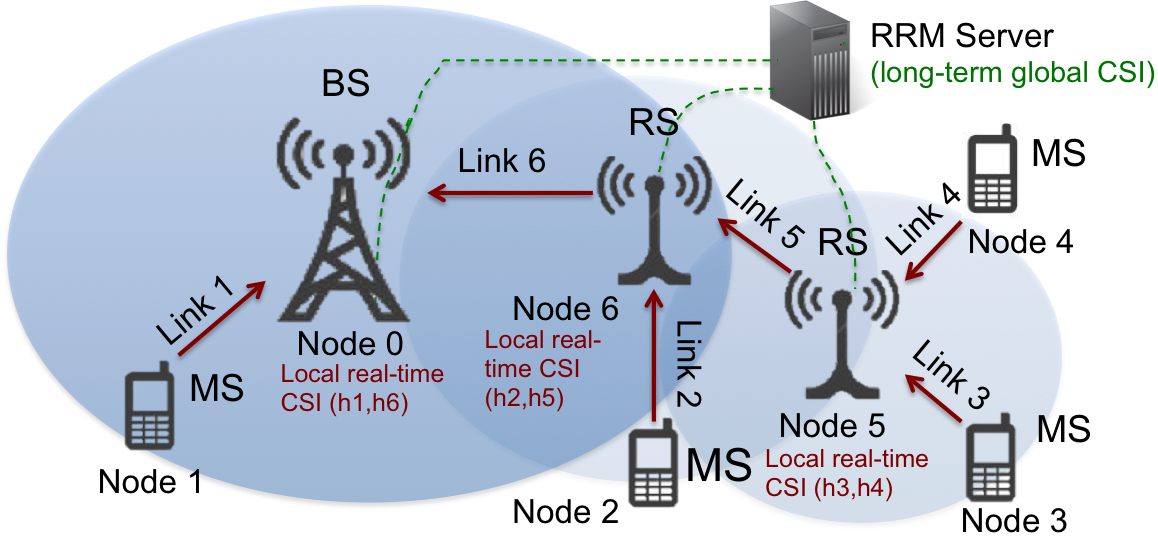
Figure 1: The topology of a wireless relay network with a radio resource management (RRM) server. The BSs and the RSs have local real-time CSI, while the RRM server has the long-term global CSI.

In this paper, we focus on the study of general cross-layer optimization for mixed timescales state processes. We first setup a stochastic optimization formulation to optimize an average network utility. The control variables are partitioned into a short-term control (adapts to fast timescale state processes) and a long-term control (adapts to slow timescale state processes) according to the information structure induced by specific network topology. These control variables are driven by mixed-timescale iterative algorithms to optimize the average network utility (objective function). An important question to the mixed timescale iterative algorithms is whether they will converge to the optimal solution. While the convergence of some iterative algorithms such as stochastic gradient [18, 19] are quite well-studied, these existing techniques considered one timescale iteration only and the convergence behavior of mixed timescale algorithms is highly non-trivial due to the mutual coupling between the short-term and long-term control variables. Specifically, there are several first order technical challenges that need to be addressed.

• Coupling in the dynamics of the long-term and short-term iterations: In most of the existing works involving multi-timescale control variables, the iterative algorithms driving different types of control variables are independent from each other. In other words, the intermediate iterates of the long-term variables in the outer-loop will not affect the convergence of the short-term variables in the inner loop. However, this decoupling is only justified when the short-term variables can converge to the optimal point arbitrarily fast or when we have closed-form solutions for the short-term variables. In general, we do not have closed-form solutions and each iteration in communication networks may also involve explicit signaling message passing. Hence, it may not be realistic to ignore the iteration dynamics in the short-term variables. Due to these couplings of the iterations between the long-term and short term variables, classical convergence proof in stochastic gradient [18, 19] or stochastic programming [20, 21, 22] cannot be applied.

• Irreducible bias to the stochastic estimator: In standard single timescale stochastic optimization with long-term control variables only, stochastic gradient [18, 19] is commonly used because the true gradient of the problem contains an expectation operator which does not have closed form expression in most cases. Using an unbiased stochastic gradient estimator [18, 19], we do not need to compute the true gradient in every iteration. If the original problem is strictly convex, the stochastic gradient algorithm will converge to the optimal solution [18, 19]. However, in the mixed timescale iterations, the convergence errors of the short-term control variables in the inner loop will induce an irreducible bias to the stochastic gradient estimator of the long-term control variables in the outer-loop. As such, standard convergence proof in stochastic gradient [18, 19] cannot be applied.

• Exogenous Stochastic Variations of the State Processes: In addition to the coupling in the mixed timescale iterations as well as the irreducible bias due to the short-term control iterations, the system states of the wireless system are also evolving stochastically. For example, the long-term state process (such as the channel path loss, the MIMO channel correlations or even the network topology) may be time-varying due to the mobility of the users in the network or shadowing process. As such, these exogenous variations will also have a profound impact on the convergence behavior of the mixed timescale iterations.

I-A Related words

In [23, 24], we have studied the convergence behavior of iterative algorithms in wireless systems under time-varying channel states. However, these works have focused on one-timescale iterations and the approach cannot be applied to address the above challenges in mixed-timescale iterations. There are also limited works on multi-timescale stochastic optimizations. In [20, 21, 22], multi-stage stochastic programming has been applied for logistic and financial planning problems. However, the problem considered has very a special form (linear program (LP)) and the solutions cannot be applied to our problems, which has a more general non-linear form. There are also some application examples [13, 14, 1, 15, 16, 17] that decompose the stochastic optimization problems into two timescale hierarchical solutions. However, all these works did not consider the tracking issues associated with exogenous variations of the problem parameters. In [25, 26], the authors studied the stochastic tracking algorithms in a regime-switching environment which is driven by a finite state two-timescale Markov chain. A dynamic step-size selection algorithm for the tracking in a regime-switching environment has been proposed in [27]. Nevertheless, a general understanding of the convergence behavior of mixed-timescale algorithms is still needed.

I-B Our contribution

In this paper, we propose an analysis framework to study the convergence behavior of mixed timescale iterative algorithms of cross-layer stochastic optimization for wireless networks. Specifically, we first introduce the cross-layer stochastic optimization framework and the variable partitioning according to the information structure available. We then consider a mixed timescale iterative algorithm and study the dynamics and coupling using continuous time stochastic differential equation (SDE). We show that the study of the convergence behavior of the mixed timescale algorithm is equivalent to the study of stochastic stability of a virtual dynamic system specified by a system of SDE. Furthermore, the optimal solution of the stochastic optimization problem is equivalent to an equilibrium point of the virtual dynamic system. As a result, the convergence behavior of the algorithm is similar to the control problem of tracking a moving target [23, 24]. Based on this insight, we derive an upper bound on the tracking error of the mixed timescale algorithms under exogenous variations of the short-term and long-term state processes. Based on the insights of the impact of exogenous variations, we propose a low complexity compensation algorithm which can substantially enhance the tracking behavior of the mixed timescale algorithms. Finally, we apply this framework to an example topology in wireless heterogeneous networks with relays. Numerical simulations verified the theoretical insights obtained and also demonstrated significant performance gain of the proposed compensation algorithms.

The paper is organized as follows. Section II illustrates the system model, where the cross-layer stochastic optimization framework and the mixed timescale stochastic approximation algorithm will be introduced. Section III studies the tracking behavior of the mixed timescale algorithm using the notion of virtual stochastic dynamic system (VSDS) and the techniques of Lyapunov stochastic stability. In Section V, a novel compensation algorithm is proposed to enhance the tracking performance. An application example on flow control and power allocation in wireless relay network is illustrated in Section VI. Section VII gives the numerical results, and we conclude the work in Section VIII.

Notations: For a scaler-valued function $F:\mathbb{R}^{n}\mapsto\mathbb{R}$, $F_{x}$ denotes the vector of its partial derivatives with respect to vector $x=(x_{1},\dots,x_{n})$, i.e., the $i$-th component of $F_{x}$ is $F_{x}^{(i)}=\frac{\partial F}{\partial x_{i}}$. For a vector-valued function $G:\mathbb{R}^{n}\mapsto\mathbb{R}^{m}$, $G_{x}$ denotes the Jacobian matrix of $G=(G^{(1)},\dots,G^{(m)})$, which is the partial derivatives of $G(\centerdot)$ with respect to vector $x$, and whose $(i,j)$-th element is given by $\frac{\partial G^{(i)}}{x_{j}}$. The notation $\lfloor x\rfloor$ denotes the largest integer that is no greater than $x$. For column vectors $x=[x_{1}\,\dots\,x_{n}]^{T}$ and $y=[y_{1}\,\dots\,y_{m}]^{T}$, $(x,y)=[x_{1}\,\dots\,x_{n}\,y_{1}\,\dots\,y_{m}]^{T}$ denotes a column vector that stacks the vectors $x$ and $y$.

II System Model

In this section, we first introduce the cross-layer stochastic optimization framework with mixed timescale exogenous random processes. We then partition the control variables into short-term and long-term controls and describe the mixed timescale iterative algorithms to track the optimal solutions of the stochastic optimization problem. Based on that, we elaborate the convergence issues induced by the exogenous random processes and formally define the tracking error between the algorithm outputs and the optimal solution.

II-A A Cross-Layer Stochastic Optimization Formulation

II-A1 Network and Mobility Model

We first discuss the system model in a wireless communication network with node mobilities. Consider a wireless network with $N_{s}$ static nodes and $N_{m}$ mobile nodes. The location of the static nodes are fixed, and the mobile nodes are randomly distributed at time $t=0$. For time $t>0$, the mobile nodes change their locations according to a widely adopted Levy walk mobility model [28, 29, 30] described as follows.

Assumption 1 (Levy walk mobility model)

Starting from time $t=0_{+}$, each mobile node chooses a random destination in a restricted region centered at the initial location and moves at a constant speed in $(0,v_{\max}]$. Upon reaching the destination, the node pauses for some time and randomly chooses a new destination and speed to go on. The travel distance and pause time at each step follow a truncated Levy distribution [29, 30].   ∎

Nodes are inter-connected through wireless links, and since the node mobility is restricted, we assume that the network topology is fixed despite the mobility of the mobile nodes. The network topology can be represented by a directed graph $\mathcal{G}=(\mathcal{N},\mathcal{L})$, where $\mathcal{N}$ is the set of nodes and $\mathcal{L}$ is the set of wireless links that connect the transmitters and the receivers. Fig. 1 illustrates an example wireless network, where $\mathcal{N}$ is the set of BS, RSs and mobile users, and $\mathcal{L}$ is the set of wireless transmission links between them.

Define the CSI for the $j$-th link as $h_{j}\in\mathcal{H}$. We adopt a fading model to the CSI $h_{j}$ as $h_{j}=h_{j}^{l}h_{j}^{s}$, where $h_{j}^{l}=c_{0}D_{j}^{-\iota}\in\mathcal{H}^{l}$ is the long-term CSI for the large-scale fading with $c_{0}$ being an antenna-gain-related constant, and $h_{j}^{s}\in\mathcal{H}^{s}$ is the short-term CSI for the small-scale fading [31, 9]. $D_{j}\geq D_{\min}$ is the distance between the $j$-th link, and $\iota$ is the path loss exponent.

II-A2 The CSI Dynamics

We specify the dynamics of the CSI $h_{j}^{s}$ and $h_{j}^{l}$ by the exogenous random processes defined below.

Definition 1 (Exogenous stochastic processes)

The short-term and long-term CSI processes $h_{j}^{s}(t)$ and $h_{j}^{l}(t)$ are driven by the following stochastic differential equations (SDE):

$$dh_{j}^{s} = -\frac{1}{2}a_{H}h^{s}dt+\sqrt{a_{H}}dW_{t},\quad h_{j}^{s}(0)=h_{0}^{s},\forall j=1,\dots,N,$$ (1)

$$dh_{j}^{l} = -c_{0}\iota D_{j}(t)^{-\iota-1}v_{j}(t)dt,\quad h_{j}^{l}(0)=h_{0}^{l},\forall j=1,\dots,N,$$ (2)

where $a_{H}>0$, $v_{j}$ is the relative speed of the $j$-th link, and $W_{t}$ is a standard Brownian motion.   ∎

The positive parameter $a_{H}$ specifies the time-correlation of the short-term exogenous processes $\{h_{j}^{s}(t)\}$, which are specified by the Ornstein-Uhlenbeck processes. $h_{j}^{s}(t)$ has a Gaussian stationary distribution and $|h_{j}^{s}|$ follows a Rayleigh distribution [8, 9]. On the other hand, defining $\epsilon(D_{\min},v_{\max})\triangleq 2c_{0}\iota D_{\min}^{-\iota-1}v_{\max}$, we have $|dh_{j}^{l}|\leq\epsilon(D_{\min},v_{\max})dt$. The parameter $\epsilon$, which is typically very small, represents the timescale of the long-term processes $\{h_{j}^{l}(t)\}$.

II-A3 Control Variables and the Problem Formulation

We assume the following information structure for the wireless communication network.

Assumption 2 (Signaling information structure)

Each node $k\in\mathcal{N}$ has knowledge of the local CSI (short-term and long-term) $(h_{j}^{s},h_{j}^{l})$ for all the links $j\in\mathcal{L}$ that connect to node $k$. On the other hand, only the global long-term CSI $h^{l}=(h_{1}^{l},\dots,h_{N_{L}}^{l})$ is known at the central controller of the network.   ∎

For example, in Fig. 1, node $5$ only has the local CSI knowledge of $h_{3}$, $h_{4}$ and $h_{5}$. Meanwhile, the RRM server has the long-term global CSI $h_{j}^{l}$ for all the nodes $j$. Note that the above assumption is quite reasonable, because in practical wireless communication networks, it is relatively easy for each node to acquire local real-time CSI but it would be difficult for the network controller to acquire the global real-time CSI.

According to the information structure assumption, the following defines the mixed timescale controls in the cross-layer optimization framework.

Definition 2 (Mixed Timescale Controls)

The system has two sets of control variables, namely the short-term control and the long-term control. The short term control is denoted by a policy $\Omega^{s}$ which maps the realization of CSI vector $h=(h_{1},\dots,h_{N})$ to an action $\theta_{x}\in\mathbb{R}_{+}^{N_{x}}$. Similarly, the long-term control is denoted by a policy $\Omega^{l}$ which maps the realization of $h^{l}=(h_{1}^{l},\dots,h_{N}^{l})$ to an action $\theta_{y}\in\mathbb{R}_{+}^{N_{y}}$ .   ∎

For example, the short-term control $\theta_{x}(t)=\Omega^{s}(h(t))$ and the long-term control $\theta_{y}(t)=\Omega^{l}(h^{l}(t))$ may correspond to the transmit power control on each wireless link and the flow control of a wireless network, respectively. The mixed timescale cross-layer stochastic optimization problem is given as follows.

Problem 1 (Mixed timescale cross-layer stochastic optimization problem)

$$\mathcal{P}_{0}(a_{H},\epsilon)=\max_{\Omega^{l},\Omega^{s}} \mathbb{E}\left[F(\theta_{x},\theta_{y};h(t))\right]$$ (3)

subject to $$w_{i}(\theta_{x},\theta_{y};h(t))=0, i=1,\dots,W_{e}$$ (4)

$$w_{i}(\theta_{x},\theta_{y};h(t))\leq 0, i=W_{e}+1,\dots,W$$ (5)

$$q_{j}(\theta_{y};h^{l}(t))\leq 0, j=1,\dots J,\forall h^{l}(t).$$ (6)

∎

$\mathcal{P}_{0}$ can be decomposed into a family of inner problems and outer problems:

Problem 2 (The inner problem)

For given $h^{s}$ and $h^{l}$,

$$\mathcal{P}_{1}(\theta_{y},h^{s},h^{l})=\max_{\theta_{x}\geq 0} F(\theta_{x},\theta_{y};h^{s},h^{l})$$ (7)

subject to $$w_{i}(\theta_{x},\theta_{y};h(t))=0, i=1,\dots,W_{e}$$ (8)

$$w_{i}(\theta_{x},\theta_{y};h(t))\leq 0, i=W_{e}+1,\dots,W$$ (9)

∎

Problem 3 (The outer problem)

For given $h^{l}$,

$$\mathcal{P}_{2}(h^{l})=\max_{\theta_{y}\geq 0} \mathbb{E}\left[\mathcal{P}_{1}(\theta_{y},h^{s},h^{l})\big{|}h^{l}\right]$$ (10)

subject to $$q_{j}(\theta_{y};h^{l}(t))\leq 0, j=1,\dots J.$$ (11)

∎

The collection of outer-problem solution $\theta_{y}^{*}(h^{l})$ for each $h^{l}$ in (10)-(11) gives the optimal long-term policy $\Omega^{l*}$. Similarly, the collection of the solution $\theta_{x}^{*}(h)$ for the inner problem $\mathcal{P}_{1}(\theta_{y}^{*},h^{l},h^{s})$ for a given $(h^{s},h^{l})$ gives the short-term optimal policy $\Omega^{s*}$.

We have the following assumption on the optimization problem $\mathcal{P}_{0}$.

Assumption 3 (Properties of $\mathcal{P}_{0}$)

We assume the following for the problem $\mathcal{P}_{0}$,

• Convex domain: The constraint domain specified by (4)-(6) is convex.

• Concave objective: Given any CSI variable $h\in\mathcal{H}$, the objective function $F(\theta_{x},\theta_{y};h)$ is strictly concave over $(\theta_{x},\theta_{y})\in\mathbb{R}_{+}^{N_{x}}\times\mathbb{R}_{+}^{N_{y}}$.

• Smoothness of $\theta_{y}^{*}(h^{l})$: Define an implicit mapping $\psi:h^{l}\mapsto\theta_{y}^{*}$ from the long-term CSI $h^{l}$ to the optimal solution $\theta_{y}^{*}(h^{l})$, i.e., $\psi(h^{l})$ solves the outer problem $\mathcal{P}_{2}(h^{l})$ in (10). There exists a constant $\varpi<\infty$, such that $\|\frac{\partial}{\partial h^{l}}\psi(\xi)-\frac{\partial}{\partial h^{l}}\psi(\xi^{{}^{\prime}})\|\leq\varpi\|\xi-\xi^{{}^{\prime}}\|$ for all $\xi,\xi^{{}^{\prime}}\in\mathcal{H}^{l}$.

∎

Note that in the problem $\mathcal{P}_{0}$, we may exclude equality constraints. However, one may always eliminate the equality constraints by either substituting them into the objective function or using the Lagrangian primal-dual method [32, 33]. Moreover, the last assumption ensures that there is no jump in the optimal solution $\theta_{y}^{*}(h^{l})$ along the long-term CSI $h^{l}$.

Due to Assumption 3, there exists a unique optimal solution $(\Omega^{s*},\Omega^{l*})$ for the problem $\mathcal{P}_{0}$.

A strong motivation to such control variable partitioning is due to the information structure of local real-time and global real-time CSI observations in wireless networks. Due to the latency involved in global signaling of wireless networks, it is not scalable to adapt all the control variables to the fast varying short-term CSI $h^{s}$. On the other hand, adapting the control only to the slow varying long-term CSI $h^{l}$ would be too conservative because it fails to exploit the real-time local CSI observations $h^{s}(t)$ for opportunistic diversity gain [31]. One favorable way to strike a balance between performance and scalability is to partition the control variables as long-term $y$ and short-term control $\theta_{y}(t)=\Omega^{s}(h(t))$. Another motivation of the control timescale separation is the layered control architecture widely adopted in the wireless system [1, 34]. For example, the short-term control policy may correspond to physical layer control (e.g. power adaptation) and the long-term control may correspond to upper layer control (such as routing and admission control).

II-B Example: Power and Flow Control in Wireless Relay Network

We illustrate the mixed timescale control with an example network with a macro BS and $N_{R}$ RSs. A set of end users $\mathcal{E}$ each transmits one data flow to the macro BS with the assistance of a collection of RSs $\mathcal{R}$. Fig. 1 illustrates a specific network topology with $N_{R}=2$ RSs, $N_{m}=4$ mobile users, $N=6$ links, and $\mathcal{L}=\{1,\dots,6\}$, $\mathcal{E}=\{1,2,3,4\}$, $\mathcal{R}=\{5,6\}$, $\mathcal{N}=\mathcal{E}\cup\mathcal{R}\cup\{0\}$, where node $0$ denotes the macro BS. Wireless links towards a common receiving node share the same time-frequency resource and multi-user detection (MUD) is used to handle cross-link interference. The maximum achievable transmission data rate at receiving node $m$ is a set of rates $c_{k}$ that satisfy the following constraints [31],

$$\sum_{k\in\mathcal{S}}c_{k}<\log\left(1+\sum_{k\in\mathcal{S}}|h_{k}|^{2}p_{k}\right),\quad\forall\mathcal{S}\subset\mathcal{L}^{+}(m)$$ (12)

where $\mathcal{L}^{+}(m)$ denotes the set of links that inject data flows to the receiving node $m$. For example, in Fig. 1, $\mathcal{L}^{+}(5)=\{3,4\}$, $\mathcal{L}^{+}(6)=\{2,5\}$ and $\mathcal{L}^{+}(0)=\{1,6\}$.

Denote $r_{j}$ as the flow rate from node $j\in\mathcal{E}$ and $\Omega^{r}(\mathbf{h}^{l})$ as the flow control policy that maps the large-scale fading variable $\mathbf{h}^{l}=(h_{1}^{l},\dots,h_{N}^{l})$ to the flow control $\mathbf{r}=(r_{1},\dots,r_{|\mathcal{E}|})$. Denote $p_{k}$ as the power allocation on link $k\in\mathcal{L}$ and $\Omega^{p}(\mathbf{h})$ as the power allocation policy that maps the CSI vector $\mathbf{h}=(h_{1},\dots,h_{N})$ to the transmission power $\mathbf{p}=(p_{1},\dots,p_{N})$. Corresponding to (3), a two-timescale stochastic maximization can be formulated as follows,

Problem 4 (Power and flow control in wireless relay network)

$$\max_{\Omega^{r},\Omega^{p}} \mathbb{E}\left[\sum_{j\in\mathcal{E}}\log(r_{j})-V\sum_{k\in\mathcal{L}}p_{k}\right]$$ (13)

subject to $$\sum_{k\in\mathcal{S}}c_{k}<\log\left(1+\sum_{k\in\mathcal{S}}|h_{k}|^{2}p_{k}\right) \forall\mathcal{S}\subset\mathcal{L}^{+}(m),\forall m\in\mathcal{R}\cup\{0\}$$ (14)

$$c_{k}=\sum_{j\in\mathcal{C}(k)}r_{j} \forall k\in\mathcal{L}$$ (15)

$$\sum_{k\in\mathcal{L}^{+}(m)}c_{k}-\sum_{k\in\mathcal{L}^{-}(m)}c_{k}=0 \forall m\in\mathcal{R}$$ (16)

where $\mathcal{C}(k)$ denotes the collection of data flows $r_{j}$ that routes through link $k$, and $\mathcal{L}^{-}(m)$ denotes the set of links that carry data flows from the transmitting node $m$.   ∎

For example, in Fig. 1, $\mathcal{C}(4)=\{r_{4}\}$, $\mathcal{C}(5)=\{r_{3},r_{4}\}$, $\mathcal{C}(6)=\{r_{2},r_{3},r_{4}\}$, and $\mathcal{L}^{-}(k)=k$, for $k=1,\dots,6$. We consider proportional fair utility [35] in the objective function of (13). Constraints (14)-(15) are the MUD capacity constraints, and constraints in (16) are the flow balance constraints, where the incoming data flow should be balanced with the outgoing data flow at each RS.

With timescale separation of the control $\Omega^{p}$ and $\Omega^{r}$, the above stochastic maximization can be decomposed into families of inner problems and outer problems.

Problem 5 (Inner power control)

For given flow data rate $\mathbf{r}$ and CSI $\mathbf{h}$,

$$Q(\mathbf{r};\mathbf{h})=\max_{\mathbf{p}\succeq 0} -V\sum_{k\in\mathcal{L}}p_{k}$$ (17)

subject to $$\sum_{k\in\mathcal{S}}c_{k}(\mathbf{r})<\log\left(1+\sum_{k\in\mathcal{S}}|h_{k}|^{2}p_{k}\right), \forall\mathcal{S}\subset\mathcal{L}^{+}(m),\forall m\in\mathcal{R}\cup\{0\}$$ (18)

where $c_{k}(\mathbf{r})=\sum_{j\in\mathcal{C}(k)}r_{j}$, $\forall k\in\mathcal{L}$.   ∎

Problem 6 (Outer flow control)

For given the large-scale fading variable $\mathbf{h}^{l}$,

$$\max_{\mathbf{r}\succeq 0} \mathbb{E}\left[\sum_{j\in\mathcal{E}}\log(r_{j})+Q(\mathbf{r};\mathbf{h})\right]$$ (19)

subject to $$\sum_{k\in\mathcal{L}^{+}(m)}c_{k}(\mathbf{r})-\sum_{k\in\mathcal{L}^{-}(m)}c_{k}(\mathbf{r})=0 \forall m\in\mathcal{R}.$$ (20)

∎

In this example, the power allocation $\mathbf{p}$ in (13) corresponds to the short-term control variable $\theta_{x}$ in (3), and the flow data rate variable $\mathbf{r}$ in (13) corresponds to the long-term control variable $\theta_{y}$. The objective function in (3) is specified by

$$F(\mathbf{p},\mathbf{r};\mathbf{h}^{s},\mathbf{h}^{l})=\sum_{j\in\mathcal{E}}\log(r_{j})-V\sum_{k\in\mathcal{L}}p_{k}.$$

Meanwhile, the inner problem constraints (8)-(9) and the outer problem constraints (11) are specified by (18) and (20), respectively. Moreover, the short-term control policy $\Omega^{s}$ in Definition 2 is specified by the power control $\mathbf{p}(t)=\Omega^{p}(\mathbf{h}(t))$ in this example. Similarly, the long-term control policy $\Omega^{l}$ is specified by $\mathbf{r}(t)=\Omega^{r}(\mathbf{h}^{l})$ here. One can check that the objective function (13) is concave in $(\mathbf{p},\mathbf{r})$ and the optimization domain specified by (14)-(16) is convex. In addition, as the Lagrangian function [32, 33] of the constrained problem (13)-(16) is continuous in $\mathbf{h}$, the smoothness condition in Assumption 3 is satisfied as well. Table I summarizes the associations between the example and the mixed timescale system model in Section II-A.

Components in the example		Corresponding components in the model
$\mathbf{h}^{s}$	Vector of small-scaling fading of the wireless links	$h^{s}$	Short-term CSI variable
$\mathbf{h}^{l}$	Vector of path loss variables of the wireless links	$h^{l}$	Long-term CSI variable
$\mathbf{h}$	The aggregated CSI	$h$	The aggregated CSI
$\Omega^{p}$	Power control policy	$\Omega^{s}$	Short-term control policy
$\Omega^{r}$	Flow control policy	$\Omega^{l}$	Long-term control policy
$\mathbf{p}$	Power allocation	$\theta_{x}$	Short-term control variable
$\mathbf{r}$	Flow rate control	$\theta_{y}$	Long-term control variable
(13)	Objective function	$F(\centerdot)$	Objective function
(18)	Constraints for the inner problem	(6)-(4)	Constraints for the inner problem (7)
(20)	Constraints for the outer problem	(11)	Constraints for the outer problem (10)

Table I: Problem associations between the example and the mixed timescale system model.

The control variable partitioning is motivated by the information structure of the wireless relay network. On one hand, the CSI $h_{k}$ is available at some corresponding receiving node $m=\{k:k\in\mathcal{L}^{+}(m)\}$. Hence the inner problem is solved locally at each receiving node $m\in\mathcal{R}\cup\{0\}$ based on real-time CSI $\{\mathbf{h}_{k}:\forall k\in\mathcal{L}^{+}(m)\}$. On the other hand, solving the outer problem with the flow balance constraints (16) (or (20)) requires a global coordination. Updating the variable $\mathbf{r}$ needs to have the global knowledge of $Q(\mathbf{r};\mathbf{h})$ and the statistics of the long-term CSI $\mathbf{h}^{l}$. It also needs to handle the global coupling induced by the flow balance constraints (16) (or (20)). As a result, explicit message passing is involved and the update can only be done in a longer timescale.

II-C Iterative Solution of the Mixed-Timescale Stochastic Optimization Problem

In this section, we discuss a stochastic gradient based two-timescale algorithm for solving $\mathcal{P}_{0}(a_{H},\epsilon)$, which consists of an inner iteration and an outer iteration. We are interested in the case where the inner and outer problems $\mathcal{P}_{1}$ and $\mathcal{P}_{2}$ do not have closed form solutions and iterations are needed to find the optimal solution.

Let $x=(\theta_{x},\lambda_{x})$ be the variable for the inner iteration, where $\theta_{x}$ is the short-term control variable in (7) and $\lambda_{x}$ is an algorithm specific auxiliary variable. Similarly, let $y=(\theta_{y},\lambda_{y})$ be the variable for the outer iteration, where $\theta_{y}$ is the long-term control variable in (10) and $\lambda_{y}$ is the auxiliary variable. The time is partitioned into frames with duration $\tau$ and slots as illustrated in Fig. 2. One frame consists of $N_{s}$ slots and local real-time CSI is acquired at each node at the beginning of each frame. During the $n_{s}$-th slot and the $n_{f}$-th frame ($n_{f}=\lfloor n_{s}/N_{s}\rfloor$), the short-term variable $x_{n_{s}}$ and long-term variable $y_{n_{f}}$ are updated according to the following mixed-timescale iterations,

$$x_{n_{s}} = \mathcal{P}_{\mathcal{X}(y)}\left[x_{n_{s}-1}+\gamma_{n_{s}}G(x_{n_{s}-1},y_{n_{f}};h^{s}(n_{f}\tau),h^{l}(n_{f}\tau))\right]$$ (21)

$$y_{n_{f}} = \mathcal{P}_{\mathcal{Y}}\left[y_{n_{f}-1}+\mu_{n_{f}}K(x_{n_{s}},y_{n_{f}-1};h^{s}(n_{f}\tau),h^{l}(n_{f}\tau))\right]$$ (22)

where $\gamma_{n_{s}}$ and $\mu_{n_{f}}$ are the step size sequences, $\mathcal{P}_{\mathcal{D}}\left[\centerdot\right]$ is an Euclidian projection onto the domain $\mathcal{D}$, and $\mathcal{X}(y)$ and $\mathcal{Y}$ are the domains related to the problem constraints (8)-(9) and (11). Fig. 2 illustrates the timescales of the iterations in (21)-(22). Each node acquires local CSI at each frame boundary and updates the short-term control variables $x_{n_{s}}$ once at each slot according to (21). The centralized controller updates the long-term variable $y_{n_{f}}$ once every frame according to (22).

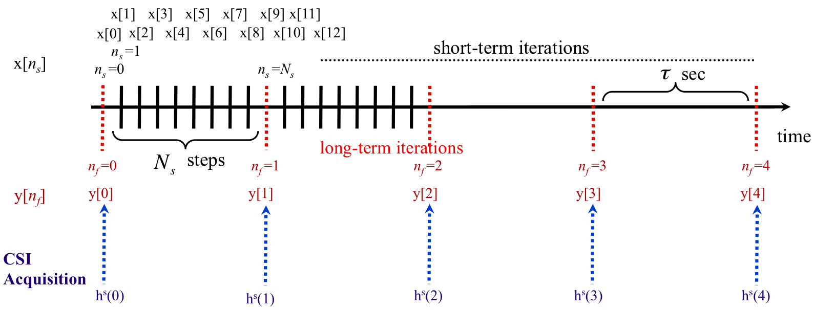
Figure 2: An illustration of the two-timescale algorithm.

In addition, we consider the following assumptions on the iterations (21)-(22).

Assumption 4 (Properties of the iterations)

Denote $\mathcal{M}(\centerdot)\triangleq(G(\centerdot),K(\centerdot))$ as the mapping of the joint iteration vector $(x_{n_{s}},y_{n_{f}})$. We assume the following properties:

• Definiteness of the iteration mappings: The Jacobian matrices of the iteration mappings $G_{x}(\centerdot)\triangleq\nabla_{x}G(\centerdot)$, $K_{y}(\centerdot)\triangleq\nabla_{y}K(\centerdot)$, and $\nabla\mathcal{M}$ have the following properties: There exists $\alpha_{x},\alpha_{y},\alpha>0$, such that $x^{T}G_{x}x\leq-\alpha_{x}\|x\|^{2}$, $y^{T}K_{y}y\leq-\alpha_{y}\|y\|^{2}$, and $(x,y)^{T}\nabla\mathcal{M}(x,y)\leq-\alpha\left(\|x\|^{2}+\|y\|^{2}\right)$ for all $(x,y)\in\left(\cup_{y\in\mathcal{Y}}\mathcal{X}(y)\right)\times\mathcal{Y}$, given any $(h^{s},h^{l})\in\mathcal{H}^{s}\times\mathcal{H}^{l}$.

• Lipschtiz continuous and bounded growth: There exist positive constants $l_{x}$ and $l_{y}$, such that $\|K(x,y_{1};\centerdot)-K(x,y_{2};\centerdot)\|\leq l_{y}\|y_{1}-y_{2}\|$, for all $y_{1}$ and $y_{2}$, and $\|K_{x}(x,y;\centerdot)x\|\leq l_{x}\|x\|$, for all $x$.

∎

Note that the first assumption is easily satisfied in a compact domain. It is needed to guarantee the iterations (21)-(22) to be stable under exogenous variation of $h(t)$, where the parameters $\alpha_{x}$ and $\alpha_{y}$ indicate the convergence speed of the inner iteration and the outer iteration, respectively, and $\alpha$ indicates the convergence speed of the whole algorithm (under one-timescale). The second assumption is a standard assumption for studying the convergence. In this paper, we are interested in the convergence of (21)-(22) to the stationary points defined as follows.

Definition 3 (Stationary points of (21)-(22))

Given $y$ and $(h^{s},h^{l})$, the partial stationary point $\hat{x}(y;h^{s},h^{l})$ of (21) is given by the solution of

$$x-\mathcal{P}_{\mathcal{X}(y)}\left[x+G(x,y;h^{s},h^{l})\right]=0.$$

Similarly, given $h^{s}$ and $h^{l}$, the stationary point $(x^{*}(h),y^{*}(h^{l}))$ of (21)-(22) is given by the solution of

$$x-\mathcal{P}_{\mathcal{X}(y)}\left[x+G(x,y;h^{s},h^{l})\right] = 0$$

$$y-\mathcal{P}_{\mathcal{Y}}\left[y+\mathbb{E}K(x,y;h^{s},h^{l})\right] = 0$$

∎

Under Assumption 4, the partial stationary point and the stationary point defined above is unique.

Remark 1 (Interpretation of the projection)

The projection $\mathcal{P}_{\mathcal{D}}(\theta)$ is to find the nearest point $x\in\mathcal{D}$ from $\theta$, i.e., $x=\mathcal{P}_{\mathcal{D}}(\theta)$ is the solution to the minimization problem $\min_{x}\|x-\theta\|_{2}^{2}$, subject to $x\in\mathcal{D}$. Note that if the constraint set is a hyper-rectangle, i.e., $\mathcal{D}=\Pi_{i=1}^{N}[a_{i},b_{i}]$, the projection can be computed by restricting each component as $a_{i}\leq x^{(i)}\leq b_{i}$. When a general constraint set $\mathcal{D}$ is considered, the projection can be computed by Lagrange multipliers[32, 33].   ∎

Remark 2 (Examples of iterative algorithms)

Different choices of the iteration mappings $G(\centerdot)$ and $K(\centerdot)$ yield different variants of the stochastic algorithm. We review a few commonly used algorithms in the following.

• Stochastic projected gradient [18, 19]: The mappings $G(\centerdot)$ and $K(\centerdot)$ are the gradients of the objective function $F(\centerdot)$ in (3). Specifically,

  $$G(x_{n_{s}-1},y_{n_{f}};h^{s}(t_{n_{f}}),h^{l}(t_{n_{f}})) = \Gamma_{x}\nabla_{x}F(x_{n_{s}-1},y_{n_{f}},h^{s}(n_{f}\tau),h^{l}(n_{f}\tau))$$ (23)

  $$K(x_{n_{s}},y_{n_{f}-1};h^{s}(t_{n_{f}}),h^{l}(t_{n_{f}})) = \Gamma_{y}\nabla_{y}F(x_{n_{s}},y_{n_{f}-1},h^{s}(n_{f}\tau),h^{l}(n_{f}\tau))$$ (24)

  where $\Gamma_{x}$ and $\Gamma_{y}$ are positive definite scaling matrices to accelerate the convergence. The iteration variables $x_{n_{s}}$ and $y_{n_{f}}$ in (21)-(22) correspond to $\theta_{x}$ and $\theta_{y}$ in (3), i.e., $\theta_{x}(n_{s})=x_{n_{s}}$ and $\theta_{y}(n_{f})=y_{n_{f}}$. In addition, the projection domains in (21)-(22) are specified by

  $$\mathcal{X}(y)=\{\theta_{x}\in\mathbb{R}_{+}^{N_{x}}:\eqref{eq:the-problem-inner-constr-1}-\eqref{eq:the-problem-inner-constr-2}\mbox{ are satisfied}\},\quad\mathcal{Y}=\{\theta_{y}\in\mathbb{R}_{+}^{N_{y}}:\eqref{eq:the-problem-outer-constr}\mbox{ is satisfied}\}.$$ (25)

  Note that $K(\centerdot)$ is a stochastic estimator of the desired gradient descent direction
  $\nabla_{y}\mathbb{E}\big{[}\max_{x}F(x,y_{n_{f}-1};h(n_{f}\tau))\big{|}h^{l}(n_{f}\tau)\big{]}$ (c.f. [36, 19]).

• Stochastic primal-dual algorithm [33, 37]: We first form a Lagrangian function of the problem in (3),

  $$L(\theta_{x},\theta_{y},\lambda_{x},\lambda_{y};h)=F(\theta_{x},\theta_{y};\centerdot)-\sum_{i}\lambda_{x,i}w_{i}(\theta_{x},\theta_{y};\centerdot)-\sum_{j}\lambda_{y,j}q_{j}(\theta_{y};\centerdot)$$

  where $\lambda_{x}\geq 0$ and $\lambda_{y}\geq 0$ are the Lagrange multipliers for the primal variables $\theta_{x}$ and $\theta_{y}$, respectively. Let $x=(\theta_{x},\lambda_{x})$ and $y=(\theta_{y},\lambda_{y})$. The mappings $G(\centerdot)$ and $K(\centerdot)$ for stochastic primal-dual algorithm are given by

  $$G(\centerdot)=\left(\begin{array}[]{c}\nabla_{\theta_{x}}L(\theta_{x},\theta_{y},\lambda_{x},\lambda_{y};h)\\ -\nabla_{\lambda_{x}}L(\theta_{x},\theta_{y},\lambda_{x},\lambda_{y};h)\end{array}\right),\quad\mbox{and}\quad K(\centerdot)=\left(\begin{array}[]{c}\nabla_{\theta_{y}}L(\theta_{x},\theta_{y},\lambda_{x},\lambda_{y};h)\\ -\nabla_{\lambda_{y}}L(\theta_{x},\theta_{y},\lambda_{x},\lambda_{y};h)\end{array}\right).$$ (26)

  In addition, the projection domains are given by

  $$\mathcal{X}(y)=\mathbb{R}_{+}^{N_{x}}\times\mathbb{R}_{+}^{W},\quad\mbox{and}\quad\mathcal{Y}=\mathbb{R}^{N_{y}}\times\mathbb{R}_{+}^{J}.$$ (27)

∎

Under Assumption 4, the convergence of (21)-(22) can be established from standard techniques [36, 19] for static CSI $h^{s}$ and $h^{l}$, as summarized below.

Theorem 1 (Convergence under static CSI $h^{s}$ and $h^{l}$)

Consider $G(\centerdot)$ and $K(\centerdot)$ are given by (23)-(24) (or (26)), with the projection domains $\mathcal{X}$ and $\mathcal{Y}$ given by (25) (or (27)). If the step size sequences $\gamma_{n_{s}}$ and $\mu_{n_{f}}$ satisfy $\sum\gamma_{n_{s}}=\infty,\sum\mu_{n_{f}}=\infty$ and $\sum\gamma_{n_{s}}^{2}<\infty,\sum\mu_{n_{f}}^{2}<\infty$, then the iteration $(x_{n_{s}},y_{n_{f}})$ in (21)-(22) converges to the stationary point $(x^{*}(h^{s},h^{l}),y^{*}(h^{l}))$. Furthermore, $(\theta_{x}^{*}(h^{s},h^{l}),\theta_{y}^{*}(h^{l}))$ solves the problem in (3).   ∎

However, when the CSI $h^{s}(t)$ and $h^{l}(t)$ are time-varying, the above convergence is not guaranteed. This is because, on one hand, the inner iteration $x_{n_{s}}$ may not converge and hence induce bias to the estimator $K(\centerdot)$ for updating $y_{n_{f}}$. On the other hand, the optimal target $y^{*}(h^{l}(t))$ is time-varying as well, and existing convergence results [18, 19] fail to apply. In this paper, we shall focus on investigating the convergence behavior of the mixed-timescale iterations (21)-(22) when the CSI $h^{l}(t)$ and $h^{s}(t)$ have mixed-timescale stochastic time-variations.

II-D Impact of Exogenous Variations and Tracking Errors

With the presence of the exogenous variations of $h(t)$, the mixed timescale iterations in (21)-(22) are continuously perturbed and the convergence to the stationary point target $(x^{*}(h(t)),y^{*}(h^{l}(t)))$ is not guaranteed. The impact of the exogenous variations can be summarized as follows,

• Impact on the inner iteration $x_{n_{s}}$: Since $h(t)$ is time-varying, $x_{n_{s}}$ needs to track the time-varying optimal point $x^{*}(h(t))$. The convergence error may depend on the relative variation speed between the iteration dynamics (21) and the exogenous variations of $h(t)$.

• Impact on the outer iteration $y_{n_{f}}$: Likewise, the optimal point $y^{*}(h^{l}(t))$ is time-varying, and $y_{n_{f}}$ may hardly reach $y^{*}(h^{l}(t))$. Moreover, the convergence error of the inner problem yields $\hat{\mathcal{P}}_{1}-\mathcal{P}_{1}\neq 0$, which induces a bias to the estimator $K(\centerdot)$ in (22).

We formally define the tracking error for the iterations (21)-(22).

Definition 4 (Tracking error)

The mean square tracking error for the short-term control variable $x$ is defined as

$$e_{x}=\lim\sup_{n_{f}\to\infty}\frac{1}{n_{f}}\sum_{i=1}^{n_{f}}\mathbb{E}\left[\|x_{iN_{s}}-\hat{x}(y_{i},h^{s}(i\tau),h^{l}(i\tau))\|^{2}\right]$$ (28)

whereas, the tracking error for the long-term control variable $y$ is defined as

$$e_{y}=\lim\sup_{n_{f}\to\infty}\frac{1}{n_{f}}\sum_{i=1}^{n_{f}}\mathbb{E}\left[\|y_{i}-y^{*}(h^{l}(i\tau))\|^{2}\right].$$ (29)

∎

In the rest of the paper, we shall study the tracking errors $e_{x}$ and $e_{y}$ under the mixed-timescale CSI $h^{s}(t)$ and $h^{l}(t)$.

III Virtual Dynamic Systems for Convergence Analysis

In this section, we derive the virtual dynamic systems for studying the tracking error of the iterations (21)-(22) under time-varying CSI. We first consider a mean continuous time dynamic system (MCTS) which captures the mean behavior of the mixed-timescale iterations in (21)-(22) under static $h^{l}$. Using SDE approximations, we then extend the results to consider the impact of time-varying $h^{l}(t)$ on the overall tracking errors and derive the VSDS.

III-A Case 1: The Mean Continuous-Time Dynamic System (MCTS) for Static $h^{l}$ and Time-varying $h^{s}(t)$

In this subsection, we consider the case for static $h^{l}$ and time-varying $h^{s}(t)$. Under time-varying $h^{s}(t)$, constant step size $\gamma$ should be used in the inner iteration (21) to track the time-varying partial stationary point $\hat{x}(t)$. On the other hand, since the stationary point $y^{*}(h^{l})$ is static, a diminishing step size $\mu_{n_{f}}$ can be used in the outer iteration (22) to assist the convergence. We derive a mean continuous-time dynamic system (MCTS) to characterize the “mean” behavior of the algorithm trajectories for (21)-(22). The MCTS is defined as follows.

Definition 5 (Mean continuous-time dynamic system (MCTS))

The state trajectory of mean continuous-time dynamic systems (MCTS) $x_{c}(t)$ and $y_{c}(t)$ are defined as the solutions to the following Skorohod reflective ordinary differential equations (ODEs) [38],

$$\dot{x}_{c} = G(x_{c},y_{c},h^{s},h^{l})+z_{x}$$ (30)

$$\dot{y}_{c} = k(y_{c},h^{l})+z_{y}.$$ (31)

where $\dot{x}_{c}\triangleq\frac{d}{dt}x_{c}(t)$, $\dot{y}_{c}\triangleq\frac{d}{dt}y_{c}(t)$. The terms $z_{x}(t)$ and $z_{y}(t)$ are the reflection terms to keep the trajectories $x$ and $y$ inside their domains $\mathcal{X}(y)$ and $\mathcal{Y}$, respectively. The function $k(\centerdot)$ is defined as

$$k(y,h^{l})\triangleq\lim_{n_{f}\to\infty}\mathbb{E}\left[K(\hat{x}(y,h(n_{f}\tau)),y,h(n_{f}\tau))\right]$$ (32)

where $K(\centerdot)$ is the iteration mapping specified in (22).   ∎

Note that since the short-term CSI process $h^{s}(t)$ in (1) is ergodic and stationary, the limit in (32) always exists.

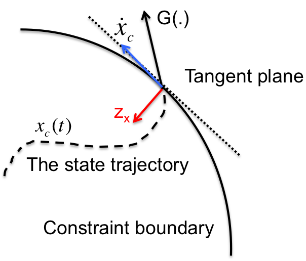
Figure 3: Illustration of the reflection term $z_{x}(t)$ when the virtual state trajectory $x_{c}(t)$ reaches the boundary of the constrain domain.

Remark 3 (Interpretation of the reflection)

The reflection term is the minimum force to restrict the trajectory inside the constraint domain. Taking $z_{x}$ for example, for $x_{c}\in\mathring{\mathcal{X}}$, in the interior of $\mathcal{X}$, $z_{x}=0$. For $x\in\partial\mathcal{X}$, the boundary of $\mathcal{X}$, $z_{x}$ lies in the convex cone generated by the inward normals on the surface of the boundary as illustrated in Fig. 3. The magnitude of $z_{x}$ is such that $G(\centerdot)+z_{x}$ lies in the tangent of the surface. Therefore, when the trajectory reaches the boundary, it can only go along on the boundary. Note that $z_{x}(t)$ and $z_{y}(t)$ can be computed using Lagrange multipliers when the constraint domain are not hyper-rectangles. Please refer to Appendix A for a derivation of the reflection terms.  ∎

In the following, we illustrate the connection between the algorithm trajectory (21)-(22) and the MCTS (30)-(31). We first derive the property of the equilibrium of MCTS.

Definition 6 (Equilibrium and partial equilibrium)

The point $(x_{c}^{*},y_{c}^{*})$ is an equilibrium of the MCTS (30)-(31) under $(h^{s},h^{l})\in\mathcal{H}^{s}\times\mathcal{H}^{l}$, if $\dot{x}_{c}=\dot{y}_{c}=0$, i.e., $G(x_{c}^{*},y_{c}^{*},h^{s},h^{l})+z_{x}=0$ and $k(y_{c}^{*},h^{l})+z_{y}=0$. In addition, for any $y_{c}\in\mathcal{Y}$, $\hat{x}_{c}(y_{c},h)$ is a partial equilibrium of the MCTS in (30) if $\dot{\hat{x}}_{c}=0$, i.e., $G(\hat{x}_{c},y_{c},h^{s},h^{l})+z_{x}=0$.   ∎

There is a strong connection between the iteration trajectory and the MCTS as summarized in the following theorem.

Theorem 2 (Connection between the algorithm trajectory and the MCTS)

Assume $\epsilon=0$ (static long-term CSI $h^{l}$). Consider $G(\centerdot)$ and $K(\centerdot)$ are given by (23)-(24) (or (26)), with the projection domains $\mathcal{X}$ and $\mathcal{Y}$ given by (25) (or (27)), and the step size sequences satisfy (i) $\gamma_{n_{f}}=\gamma$ for some small enough $\gamma>0$, and (ii) $\sum\mu_{n_{f}}=\infty$ and $\sum\mu_{n_{f}}^{2}<\infty$. In addition, the short-term CSI timescale is much slower than the algorithm timescale, i.e., $a_{H}\tau\ll\gamma$. Then the algorithm iteration trajectory $(x_{n_{s}(t)},y_{n_{f}(t)})$ in (21)-(22) converges to the virtual state trajectory of the MCTS $(x_{c}(t),y_{c}(t))$ in (30)-(31) in probability, i.e., for any $\eta>0$,

$$\lim\sup_{t\to\infty}\mbox{Pr}\left\{\|x_{n_{s}(t)}-x_{c}(t)\|>\eta\right\}=0,\;\mbox{and }\;\lim\sup_{t\to\infty}\mbox{Pr}\left\{\|y_{n_{f}(t)}-y_{c}(t)\|>\eta\right\}=0$$

where $n_{s}(t)=\lfloor tN_{s}/\tau\rfloor$ and $n_{f}(t)=\lfloor t/\tau\rfloor$.   ∎

The theorem is established using stochastic approximation [18, 19]. We sketch the proof in Appendix B.

From Theorem 2, the study of the algorithm convergence is equivalent to the study of the stability of the MCTS. The MCTS in (30)-(31) can be viewed as the desired “mean” trajectory in the continuous-time counter-part of the discrete-time algorithm iterations (21)-(22), which has filtered the noisy perturbation induced by the exogenous variation of $h^{s}(t)$ in the estimator $K(\centerdot)$. Hence, the stability of the MCTS provides a necessary and sufficient condition for the convergence of the original iterations (21)-(22) under static $h^{l}$.

Note that, under Assumption 4, the MCTS (22) is asymptotically stable [39], i.e., $y_{c}(t)\to y^{*}$ as $t\to\infty$. Therefore, from Theorem 2, we have the following result on the convergence under static $h^{l}$ and time-varying $h^{s}(t)$ when the CSI timescale is sufficiently slower than the algorithm timescale.

Corollary 1 (Convergence under static $h^{l}$ and slow time-varying $h^{s}(t)$)

For sufficiently fast algorithm iteration, i.e., $a_{H}\tau\ll\gamma$, the iteration $(x_{n_{s}(t)},y_{n_{f}(t)})$ in (21)-(22) converges to $(x^{*}(t),y^{*})$ almost surely, i.e., $\|x_{n_{s}(t)}-x^{*}(t)\|\to 0$ and $\|y_{n_{f}(t)}-y^{*}\|\to 0$ almost surely, as $t\to\infty$.   ∎

Fig. 4.a) illustrates the relationships between the algorithm iterations, the virtual dynamic system MCTS and the moving equilibrium of the MCTS for the case when both $h^{s}$ and $h^{l}$ are static. The virtual system MCTS as well as the algorithm iterations $x_{n_{s}}$ and $y_{n_{f}}$ would eventually converge to the static equilibrium $(x^{*}(h),y^{*}(h^{l}))$. Fig. 4.b) illustrates the case for static $h^{l}$ and slowly time-varying $h^{s}(t)$. For variable $y$, there is a static equilibrium $y^{*}(h^{l})$ of the virtual dynamic system MCTS, and the virtual system state $y_{c}(t)$ converges to the static target $y^{*}(h^{l})$. For variable $x$, the trajectory of the partial equilibrium $\hat{x}(y_{c}(t),h(t))$ is driven by the time-varying $y_{c}(t)$ and $h(t)$, and it eventually converges to the trajectory of the moving equilibrium $x^{*}(h(t))$, as $y_{c}(t)$ converges to $y^{*}(h^{l})$. Meanwhile, the dynamics of the MCTS tracks the moving partial equilibrium $\hat{x}(y_{c}(t),h(t))$. For both $x$ and $y$, the algorithm iterations $x_{n_{s}}$ and $y_{n_{f}}$ in (21)-(22) roughly follow the dynamics of the virtual system MCTS. However, the case is different under time-varying $h^{l}(t)$ and $h^{s}(t)$, as illustrated in Fig. 4.c). The equilibrium $y^{*}(h^{l}(t))$ of the virtual dynamic system MCTS moves around and $y_{c}(t)$ never converges. Affected by the time-varying $y^{*}(t)$ and the error gap $y_{c}(t)-y^{*}(t)$, the dynamics of the partial equilibrium $\hat{x}(y_{c}(t),h(t))$ cannot converge to the optimal trajectory $x^{*}(h(t))$. Nevertheless, the algorithm iterations $x_{n_{s}}$ and $y_{n_{f}}$ in (21)-(22) still follow the behavior of the virtual dynamic system MCTS.

In the next section, we extend the MCTS equivalence framework to the case with time-varying $h^{l}(t)$ and $a_{H}\tau\approx\gamma$.

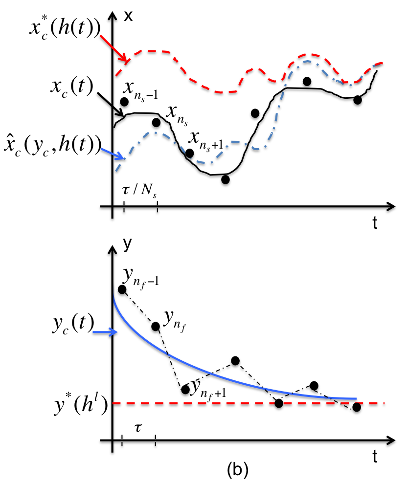
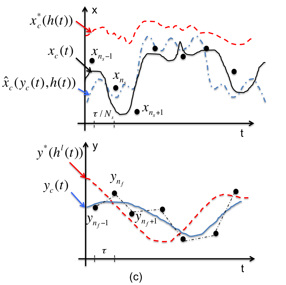
Figure 4: Illustrations of the algorithm iterations, the virtual dynamic system MCTS and the moving equilibrium of the MCTS. (a) illustrates the case for static $h^{l}$ and $h^{s}$, (b) illustrates the case for static $h^{l}$ and time-varying $h^{s}(t)$, and (c) illustrates the case of time-varying $h^{l}(t)$ and $h^{s}(t)$.

III-B Case 2: Virtual Stochastic Dynamic System for Time-Varying $h^{s}(t)$ and $h^{l}(t)$

When $h^{l}(t)$ is time-varying, the algorithm iterations $(x_{n_{s}},y_{n_{f}})$ in (21)-(22) should continuously track the time-varying partial optimal point $(\hat{x}(t),y^{*}(t))$, which is a moving target as illustrated in Fig. 4.b). As such, we consider constant step size $\gamma_{n_{s}}=\mu_{n_{f}}=\gamma$ instead of diminishing step size.

We need to first quantify the dynamics of the moving partial equilibrium $(\hat{x}(t),y^{*}(t))$ from the MCTS under the variation of $h^{l}(t)$. Using the CSI timescale separation property $\epsilon\ll a_{H}$ for $h^{s}(t)$ and $h^{l}(t)$, the dynamics of the moving target $(\hat{x}(t),y^{*}(t))$ is given by:

Lemma 1 (Dynamics of the moving partial equilibrium)

Define $\widetilde{G}(x,y,h^{s},h^{l})=G(x,y,h^{s},h^{l})+z_{x}$. The dynamics of $\hat{x}_{c}(t)$ and $y_{c}^{*}(t)$ are given by

$$d\hat{x}_{c} = -\widetilde{G}_{x}^{-1}(\hat{x}_{c}(y_{c},\centerdot),y_{c},h^{s},h^{l})\left[\widetilde{G}_{h^{s}}(\hat{x}_{c}(y_{c},\centerdot),y_{c},h^{s},h^{l})dh^{s}+\widetilde{G}_{y}(\hat{x}_{c}(y_{c},\centerdot),y_{c},h^{s},h^{l})dy\right]$$ (33)

$$dy_{c}^{*} = \psi_{h^{l}}(h^{l})dh^{l}$$ (34)

where $\widetilde{G}_{x}(\centerdot)\triangleq\frac{\partial}{\partial x}\widetilde{G}(x_{c},y_{c},h^{s},h^{l})$, $\widetilde{G}_{y}(\centerdot)\triangleq\frac{\partial}{\partial y}\widetilde{G}(x_{c},y_{c},h^{s},h^{l})$, $\widetilde{G}_{h^{s}}(\centerdot)\triangleq\frac{\partial}{\partial h^{s}}\widetilde{G}(x_{c},y_{c},h^{s},h^{l})$ and $\psi_{h^{l}}=\frac{\partial}{\partial h^{l}}\psi(h^{l})$ as defined in Assumption 4.   ∎

Proof:

Please refer to Appendix C for the proof. ∎

With the notion of MCTS and the dynamic of the moving equilibrium in (33)-(34), the instantaneous tracking errors can be expressed as

$$x_{n_{s}(t)}-\hat{x}_{c}(t) = (x_{n_{s}(t)}-x_{c}(t))+(x_{c}(t)-\hat{x}_{c}(t))$$ (35)

$$= \sqrt{\gamma}\widetilde{x}_{c}^{\gamma}(t)+\widetilde{x}_{c}^{e}(t)$$

and

$$y_{n_{f}(t)}-y_{c}^{*}(t) = (y_{n_{f}(t)}-y_{c}(t))+(y_{c}(t)-y_{c}^{*}(t))$$ (36)

$$= \sqrt{\gamma}\widetilde{y}_{c}^{\gamma}(t)+\widetilde{y}_{c}^{e}(t)$$

where $\widetilde{x}_{c}^{\gamma}(t)\triangleq\frac{1}{\sqrt{\gamma}}\left(x_{n_{s}(t)}-x_{c}(t)\right)$ and $\widetilde{y}_{c}^{\gamma}(t)\triangleq\frac{1}{\sqrt{\gamma}}\left(y_{n_{f}(t)}-y_{c}(t)\right)$ are the scaled error gap between the iteration trajectory (21)-(22) and the MCTS, and $\widetilde{x}_{c}^{e}(t)\triangleq x_{c}(t)-\hat{x}_{c}(t)$ and $\widetilde{y}_{c}^{e}(t)\triangleq y_{c}(t)-y_{c}^{*}(t)$ are the scaled tracking error from the MCTS to the moving partial equilibrium (33)-(34).

Even though it is very hard to quantify the tracking errors $x_{n_{s}(t)}-\hat{x}_{c}(t)$ and $y_{n_{f}(t)}-y_{c}^{*}(t)$, we can try to study the distributions of the decomposed error states $\widetilde{x}_{c}^{\gamma}(t)$, $\widetilde{x}_{c}^{e}(t)$, $\widetilde{y}_{c}^{\gamma}(t)$, and $\widetilde{y}_{c}^{e}(t)$ with the help of a virtual dynamic system defined in the following.

Define a joint virtual state $u(t)=(\widetilde{x}_{c}(t),\widetilde{y}_{c}(t),\widetilde{x}_{c}^{e}(t),\widetilde{y}_{c}^{e}(t),\widetilde{h}^{s}(t))\in\mathbb{R}^{2N_{x}+2N_{y}+N}$, where $\widetilde{x}_{c},\widetilde{x}_{c}^{e}\in\mathbb{R}^{N_{x}}$, $\widetilde{y}_{c},\widetilde{y}_{c}^{e}\in\mathbb{R}^{N_{y}}$ and $\widetilde{h}^{s}(t)$ is a short-term virtual CSI state with initial value $\widetilde{h}^{s}(0)=h^{s}(0)$. Correspondingly, define a virtual long-term CSI state $\widetilde{h}^{l}(t)$ as the solution of $d\widetilde{h}^{l}=-\frac{\tau}{N_{s}\gamma}H_{L}(t)dt$, with initial value $\widetilde{h}^{l}(0)=h^{l}(0)$, where $H_{L}(t)$ is an $N\times N$ diagonal matrix, with the $j$-th diagonal element being $c_{0}\iota D_{j}(t)^{-\iota-1}v_{j}(t)$. We use a short hand notation $\widetilde{G}_{x}^{-1}\widetilde{G}_{h^{s}}(\centerdot)$ to stand for the matrix $\widetilde{G}_{x}^{-1}(x_{c},y_{c},h^{s},h^{l};t)\widetilde{G}_{h^{s}}(x_{c},y_{c},h^{s},h^{l};t)$ from (34). The VSDS is defined as follows.

Definition 7 (Virtual stochastic dynamic system (VSDS))

The virtual state trajectory of the VSDS $u(t)$ is characterized by the following SDE:

$$du=U_{1}(t,u)dt+U_{2}(t,u)dW_{t}+dZ_{u}$$ (37)

where

$$U_{1}(t,u)\triangleq\left(\begin{array}[]{c}G_{x}(x_{c},y_{c},\widetilde{h}^{s},\widetilde{h}^{l})\widetilde{x}_{c}+G_{y}(x_{c},y_{c},\widetilde{h}^{s},\widetilde{h}^{l})\widetilde{y}_{c}\\ N_{s}^{-1}K_{x}(\hat{x}_{c},y_{c},\centerdot)(\widetilde{x}_{c}+\widetilde{x}_{c}^{e})+N_{s}^{-1}K_{y}(\hat{x}_{c},y_{c},\centerdot)\widetilde{y}_{c}\\ G(x_{c},y_{c},\widetilde{h}^{s},\widetilde{h}^{l})-\frac{1}{2}\frac{a_{H}\tau}{N_{s}\gamma}\widetilde{G}_{x}^{-1}\widetilde{G}_{h^{s}}(\centerdot)\widetilde{h}^{s}+\widetilde{G}_{x}^{-1}\widetilde{G}_{y}(\centerdot)N_{s}^{-1}k(y_{c},\widetilde{h}^{l})\\ N_{s}^{-1}k(y_{c},\widetilde{h}^{l})+\frac{\tau}{N_{s}\gamma}\psi_{h^{l}}(\widetilde{h}^{l})H_{L}(t)\\ -\frac{1}{2}\frac{a_{H}\tau}{N_{s}\gamma}\widetilde{h}^{s}\end{array}\right),$$

and

$$U_{2}(t,u)\triangleq\left(\begin{array}[]{ccccc}\mathbf{0}_{N_{x}\times N_{x}}&&&\ldots&\mathbf{0}_{N_{x}\times N}\\ &\sqrt{\tau N_{s}^{-1}}\Sigma^{\frac{1}{2}}(y_{c};\widetilde{h}^{l})&&&\vdots\\ &&\mathbf{0}_{N_{x}\times N_{x}}&&\sqrt{\frac{a_{H}\tau}{N_{s}\gamma}}\widetilde{G}_{x}^{-1}\widetilde{G}_{h^{s}}\\ \vdots&&&\mathbf{0}_{N_{y}\times N_{y}}&\mathbf{0}_{N_{x}\times N_{x}}\\ \mathbf{0}&\dots&&&\sqrt{\frac{a_{H}\tau}{N_{s}\gamma}}\mathbf{I}_{N}\end{array}\right).$$

Moreover, $W_{t}$ is a $(2N_{x}+2N_{y}+N)$-dimensional Brownian motion, $dZ_{u}=\big{(}\mathbf{0}_{N_{x}},dZ_{x}+dZ_{y},$
$\widetilde{G}_{x}^{-1}\widetilde{G}_{y}(\centerdot)dZ_{y},dZ_{y},\mathbf{0}_{N}\big{)}$ is the reflection term, and $\Sigma(y_{c};\widetilde{h}^{l})$ is the covariance matrix for the stochastic estimator $K(\centerdot)$ in (22).   ∎

As is summarized in the following theorem, the VSDS provides a weak convergence limit (convergence in distribution, c.f. [36, 19]) to the dynamics of the error gaps $\widetilde{x}_{c}^{\gamma}(t)$, $\widetilde{x}_{c}^{e}(t)$, $\widetilde{y}_{c}^{\gamma}(t)$, and $\widetilde{y}_{c}^{e}(t)$, when $\gamma\to 0$.

Theorem 3 (Algorithm Tracking Errors and VSDS)

Assuming CSI timescale separation for $h^{l}(t)$ and $h^{s}(t)$, i.e., $\epsilon\ll a_{H}$, the joint state $(\widetilde{x}_{c}^{\gamma},\widetilde{y}_{c}^{\gamma},\widetilde{x}_{c}^{e},\widetilde{y}_{c}^{e},\widetilde{h}^{s})$ weakly converges to $u(t)$, as $\gamma\to 0$, which is the solution to the VSDS in (37).   ∎

Proof:

Please refer to Appendix D for the proof. ∎

The above results allow us to work with the VSDS in (37) to study the convergence of the mixed timescale tracking algorithm (21)-(22). The VSDS provides statistical dynamics for the decomposed tracking error states. We formally summarize the connection between the VSDS and the tracking errors for the mixed-timescale iterations (21)-(22) in the following theorem.

Corollary 2 (Connections between the VSDS and the iterations)

Assuming CSI timescale separation for $h^{l}(t)$ and $h^{s}(t)$, i.e., $\epsilon\ll a_{H}$, the tracking errors for the algorithm iterations (21)-(22) defined in (28) and (29) can be upper bounded from $u(t)$, i.e.,

$$e_{x}\leq\lim\sup_{t\to\infty}\frac{1}{t}\max\left(\gamma,1\right)\int_{0}^{t}\mathbb{E}\left[\|\widetilde{x}_{c}(s)\|^{2}+\|\widetilde{x}_{c}^{e}(s)\|^{2}\right]ds$$

and

$$e_{y}\leq\lim\sup_{t\to\infty}\frac{1}{t}\max\left(\gamma,1\right)\int_{0}^{t}\mathbb{E}\left[\|\widetilde{y}_{c}(s)\|^{2}+\|\widetilde{y}_{c}^{e}(s)\|^{2}\right]ds$$

where $\widetilde{x}_{c}(t)$, $\widetilde{x}_{c}^{e}(t)$, $\widetilde{y}_{c}(t)$, and $\widetilde{y}_{c}^{e}(t)$ are the components of the joint state $u(t)$ in the VSDS (37).   ∎

Corollary 2 can be seen from the tracking errors (35)-(36) and the results in Theorem 3. With Theorem 2, we can focus on studying the stochastic stability (formally defined in Section IV-A) of the VSDS in (37) in order to understand the convergence behavior of the mixed timescale iterations in (21) and (22).

Moreover, the VSDS suggests that the tracking errors consist of two parts: (i) the steady state error $\gamma\|\widetilde{x}_{c}\|^{2}$ and $\gamma\|\widetilde{y}_{c}\|^{2}$, which are the mean square error gaps between the iteration trajectory $(x_{n_{s}},y_{n_{f}})$ in (21)-(22) and the MCTS $(x_{c}(t),y_{c}(t))$ in (30)-(31), and (ii) the mean tracking error $\|\widetilde{x}_{c}^{e}(t)\|^{2}$ and $\|\widetilde{y}_{c}^{e}(t)\|^{2}$, which are the mean square distances between the MCTS and the target moving partial equilibrium $(\hat{x}(t),y^{*}(t))$ in (33)-(34). Note that when $h^{l}$ is static, i.e., $H_{L}(t)\equiv 0$, the tracking error $\widetilde{y}_{c}^{e}(t)$ in the VSDS converges to 0, and hence, there is only steady state error $\gamma\|\widetilde{y}_{c}\|^{2}$ (due to constant step size) for the long-term variable $y$.

IV Convergence Analysis of Mixed Timescale Iterations

In this section, we derive the tracking error bound of the mixed timescale iteration (21)-(22) by studying the VSDS obtained from Section III. We first briefly review the Lyapunov stochastic stability techniques. By studying the stability of the VSDS, we then derive a sufficient condition for the convergence of the mixed-timescale algorithm. Moreover, we obtain a tracking error bound in terms of the parameters of the exogenous process $h(t)$.

IV-A Preliminary Results on the Lyapunov Stochastic Stability

It is very hard to derive the exact solutions for the VSDS. Instead, we are interested in the expected upper bound value of the joint state $\|u(t)\|$, which represents the aggregated tracking error $e_{x}+e_{y}$ of the iterations. This is captured by the stochastic stability in mean square defined as follows.

Definition 8 (Stochastic stability in mean square)

Given any initial state $u(0)\in\mathcal{U}$, the stochastic process $u(t)$ is globally stochastically stable in mean square, if there exists $0\leq\delta<\infty$, such that $\lim\sup_{t\to\infty}\frac{1}{t}\int_{0}^{t}\mathbb{E}\left\|u(\tau)\right\|^{2}d\tau\leq\delta.$   ∎

We use a Lyapunov method to study the stochastic stability of $u(t)$. Define a non-negative function $V(u)=\frac{1}{2}u^{T}u$ along the trajectory of $u(t)$. The function has the property that $V(u)\sim\|u\|^{2}$, which plays the role of an energy function, where a larger $\|u\|$ gives a larger function value. We summarize the main techniques of stochastic stability analysis as follows.

Definition 9 (Lyapunov drift operator)

Consider a stochastic process $u(t)$ and a real-valued Lyapunov function $V(u)$. The Lyapunov drift operator is an infinitesimal estimator on $V(\centerdot)$ defined as $\widetilde{\mathcal{L}}V(u)=\lim_{\delta\downarrow 0}\frac{1}{\delta}\left[\mathbb{E}\left[V(u(t+\delta)|V(u(t)\right]-V(u(t))\right].$   ∎

Lemma 2 (Stochastic Stability from Lyapunov Drift)

Consider a function $f(u)$ that satisfies $f(u)\geq a\|u\|^{r}$ for all $u\in\mathcal{U}$, and some $a,r>0$. Suppose the stochastic Lyapunov drift of the process $u(t)$ has the following property

$$\mathcal{\widetilde{L}}V(u)\leq-f(u)+g(s)$$ (38)

for all $u\in\mathcal{U}$, where $s(t)$ is a stochastic process that satisfies $\lim\sup_{t\to\infty}\frac{1}{t}\int_{0}^{t}\mathbb{E}\left[g(s(\tau))\right]d\tau\leq d$ for some function $g(s)$ and $d<\infty$. Then the process $u(t)$ is stochastically stable, and

$$\lim\sup_{t\to\infty}\frac{1}{t}\int_{0}^{t}\mathbb{E}\|u(\tau)\|^{r}d\tau\leq\frac{d}{a}.$$

∎

The above result is based on the Foster-Lyapunov criteria for continuous time processes in [40] and is a simple extension of the results in [24, Theorem 2]. The advantage of the Lyapunov method enables a qualitative analysis of the SDE without explicitly solving it. Using such a technique, we derive the stability results for the mixed timescale algorithm in the following.

IV-B Stability of the Mixed-Timescale Algorithm

Corresponding to stability of a random process, we define the iteration stability as follows.

Definition 10 (Stability of the iteration)

The iterations (21) and (22) are stable if the corresponding tracking error defined in (28) and (29) are bounded, i.e., there exists a $B<\infty$, such that $e_{x}+e_{y}\leq B$.   ∎

Note that due to the stochastic iterations, the tracking errors defined in (28) and (29) may be unbounded statistically. To study the algorithm stability, we can equivalently investigate the stability of the VSDS $u(t)$. Towards this end, we first construct a Lyapunov drift $\mathcal{\widetilde{L}}V(u)$ on the trajectory of the VSDS in (37). We then proceed to find a function $g(s)$ that satisfies condition (38). Finally, we use Theorem 2 to obtain the stability result.

We summarize the sufficient conditions of the stability of the mixed timescale algorithm as follows.

Theorem 4 (Sufficient conditions for the algorithm stability)

Assume CSI timescale separation for $h^{l}(t)$ and $h^{s}(t)$, i.e., $\epsilon\ll a_{H}$. Suppose that there exist $0<v_{H},v_{y}<\infty$, such that $\|G_{x}^{-1}G_{h^{s}}\|\leq v_{H}$ and $\|G_{x}^{-1}G_{y}\|\leq v_{y}$. Then the sufficient condition for the algorithm to be stable is given by

$$\alpha N_{s}\left(8\alpha_{x}-\frac{a_{H}\tau}{N_{s}\gamma}v_{H}^{2}\right)-2l_{x}^{2}-2l_{y}^{2}v_{y}^{2}>0.$$ (39)

∎

Proof:

Please refer to Appendix E for the proof. ∎

The above results have several implications on the convergence.

• Convergence of the inner problem: The term $N_{s}\left(8\alpha_{x}-\frac{a_{H}\tau}{N_{s}\gamma}v_{H}^{2}\right)$ specifies the convergence behavior of the inner problem. Recall that the parameter $a_{H}$ controls the variation speed of the fast changing CSI $h^{s}(t)$, $\alpha_{x}$ represents the convergence rate of the inner problem, $\tau$ is the frame duration, $N_{s}$ is the number of slots per frame, and $\gamma$ is the step size. As such, for a given $a_{H}$, we need to have sufficiently fast inner iterations ($\alpha_{x}$) or sufficient number of slots per frame ($N_{s}$) in order to have bounded tracking error.

• Convergence of the outer problem and the coupling effect: The convergence of the inner problem and outer problem is coupled together. The stability of the inner problem (a positive $8\alpha_{x}-\frac{a_{H}\tau}{N_{s}\gamma}v_{H}^{2}$) is a premise of the stability of the whole algorithm. To achieve the stability, we desire small $v_{H}$ and $l_{x}$, which represent the sensitivity of the partial stationary point $\hat{x}$ w.r.t. the change of $h^{s}(t)$. On the other hand, we also want the parameters $l_{y}$ and $v_{y}$ to be small, which means that $y^{*}$ shall not be quite sensitive to the bias induced by the tracking error $x_{n_{s}}-\hat{x}(y_{n_{f}},\centerdot)$.

• Impact from the iteration timescale: One can reduce the frame duration $\tau$, increase the number of slots $N_{s}$ per frame, or increase the step size $\gamma$ to enhance the stability of the overall algorithm. However, shortening the frame duration $\tau$ may result in a larger amount of signaling overhead to update the long-term variable $y_{n_{f}}$ and the acquisition of local CSI $h^{s}(n_{f}\tau)$; increasing the number of slots $N_{s}$ yields a higher computational complexity; and moreover, a large step size $\gamma$ may give larger steady state error $\mathcal{O}(\gamma)$ for the discrete-time trajectory.

IV-C Upper Bound of the Tracking Error

Stability is only a weak result of convergence. We are interested in the tracking error bound of the algorithm. Under the sufficient condition specified in (39), using the Lyapunov technique in Lemma 2, we study the result on the upper bound of the tracking errors $e_{x}$ and $e_{y}$.

Theorem 5 (Upper bound of the tracking error)

Assume the conditions in Theorem 4. If $\overline{\Sigma}\triangleq\lim\sup_{t\to\infty}\frac{1}{t}\int_{0}^{t}\mbox{tr}\left(\Sigma(y^{*}(h^{l}(\tau)))\right)d\tau<\infty$, the tracking errors $e_{x}$ and $e_{y}$ are given by:

$$e_{x}+e_{y}\leq\frac{\eta}{\rho}\left(\tau\overline{\Sigma}+C\right)$$ (40)

where $\rho=\mathcal{O}\left(N_{s}\alpha^{2}\alpha_{x}\alpha_{y}\right)$, $\eta=\mathcal{O}\left(\sqrt{N_{s}^{2}\alpha_{x}^{2}+\alpha^{2}}\right)$, $C=\frac{a_{H}\tau}{\gamma}N(1+v_{H}^{2})+\mathcal{O}(\epsilon^{2}\varpi^{2}\tau^{2}\gamma^{-2})$, and $N$ is the dimension of the CSI vector $h^{s}$.   ∎

Proof:

Please refer to Appendix F for the proof. ∎

The above result shows that the upper bound of the tracking error depends on several important parameters, such as the timescale parameter $a_{H}$ for $h^{s}(t)$, the sensitivities $v_{H}$ and $v_{y}$ of the stationary points $\hat{x}$ and $y^{*}$, respectively, as well as the sensitivities $\varpi$ of $y^{*}(h^{l})$ over $h^{l}$. A faster time-varying scenario corresponds to larger $a_{H}$, which result in a larger tracking error bound. In addition, we can observe the followings.

• Special case for static $h^{l}$ and $h^{s}$: Under static CSI, where the CSI timescale parameters $a_{H}=\epsilon=0$, we have the term $C=0$ in the error bound. The tracking error is governed by the steady state error $\frac{\eta}{\rho}\tau\overline{\Sigma}$ due to the constant step size $\gamma$. Note that if diminishing step size is used for the outer iteration (22), i.e., $\mu_{n_{f}}\to 0$, the tracking error bound in (40) becomes $0$. This corresponds to the case in Fig. 4.a).

• Special case for static $h^{l}$ and time-varying $h^{s}(t)$: Under static $h^{l}$, where long-term CSI timescale parameter $\epsilon=0$, the term $C$ decreases, because the term $\mathcal{O}(\epsilon^{2}\varpi^{2}\tau^{2}\gamma^{-2})$ becomes $0$. In particular, if diminishing step size is used for the outer iteration (22), i.e., $\mu_{n_{f}}\to 0$, the error bound becomes $\frac{\eta}{\rho}C$ and is mainly contributed by the tracking error in the inner iteration. This corresponds to the case in Fig. 4.b).

• Impact of the algorithm parameters: When the CSI $(h^{s},h^{l})$ is fast changing, i.e., the CSI timescale parameters $a_{H}$ and $\epsilon$ are large, one can reduce the frame duration $\tau$, increase the number of slots $N_{s}$ per frame, or increase the step size $\gamma$ to reduce the tracking error, with the price of larger signaling overhead, higher computational complexity and larger steady state error $\mathcal{O}(\gamma)$ as discussed in Section IV-B.

V Compensation for Mixed Timescale Iterations

In the previous sections, we have analyzed the convergence behavior of the iteration (21)-(22) under mixed timescale time-varying CSI $h(t)$. In this section, we shall enhance the algorithm for better tracking performance. Since the convergence of the outer long-term variable $y$ depends on the convergence of the inner problem, it is essential to accelerate the convergence of the short-term variable $x_{n_{s}}$. Towards this end, we introduce a compensation term in the algorithm (21) to offset the exogenous disturbance to the VSDS in (37).

V-A Adaptive Compensations for the Time-varying CSI

Recall that in the mixed timescale iterations (21)-(22), the inner iteration tracks the moving target $\hat{x}(t)$ driven by the time-varying $h(t)$ and $y(t)$. On the other hand, the outer iteration tracks the moving target $y^{*}(t)$ driven by $h^{l}(t)$. As a result, when $h(t)$ and $y(t)$ are time-varying, they generate disturbance to the tracking iterations (21) and (22). This can be seen from the dynamics of the error states $\widetilde{x}_{c}^{e}(t)$ and $\widetilde{y}_{c}^{e}(t)$ in the VSDS in (37) (c.f. equations (75) and (76))

$$d\widetilde{x}_{c}^{e} = G(x_{c},y_{c},\widetilde{h}^{s},\widetilde{h}^{l})dt\underbrace{+\widetilde{G}_{x}^{-1}\widetilde{G}_{h^{s}}(\centerdot)d\widetilde{h}^{s}}_{\mbox{\scriptsize\ exogenous disturbance from }\widetilde{h}^{s}(t)}\underbrace{+\widetilde{G}_{x}^{-1}\widetilde{G}_{y}(\centerdot)dy_{c}}_{\mbox{\scriptsize\ distrubance from }y(t)}$$ (41)

$$d\widetilde{y}_{c}^{e} = N_{s}^{-1}k(y_{c},\widetilde{h}^{l})dt\underbrace{-\psi_{h^{l}}(h^{l})d\widetilde{h}^{l}}_{\mbox{\scriptsize\ exogenous disturbance from }\widetilde{h}^{l}(t)}.$$ (42)

Note that, from Theorem 2 and Corollary 1, when $d\widetilde{h}^{l}=0$, the error dynamic system (42) is asymptotically stable and the error state $\widetilde{y}_{c}^{e}(t)$ converges to 0. In addition, when $d\widetilde{h}^{s}=0$, the system (41) is stable and the error state $\widetilde{x}_{c}^{e}(t)$ converges to $0$ as well. However, with the presence of the exogenous disturbance $d\widetilde{h}^{s}$ and $d\widetilde{h}^{l}$, the error states $\widetilde{x}_{c}^{e}(t)$ and $\widetilde{y}_{c}^{e}(t)$ are continuously disturbed and may fail to converge to the origin. This is illustrated in Fig. 5.

            

            

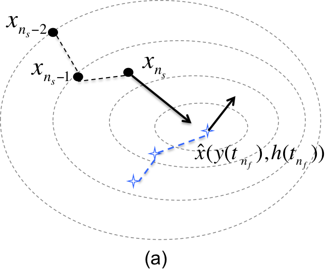
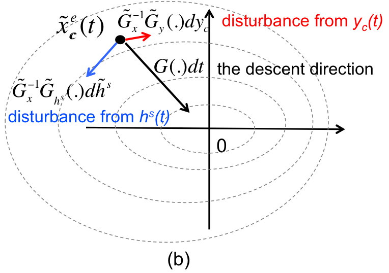
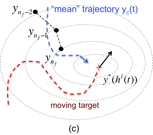
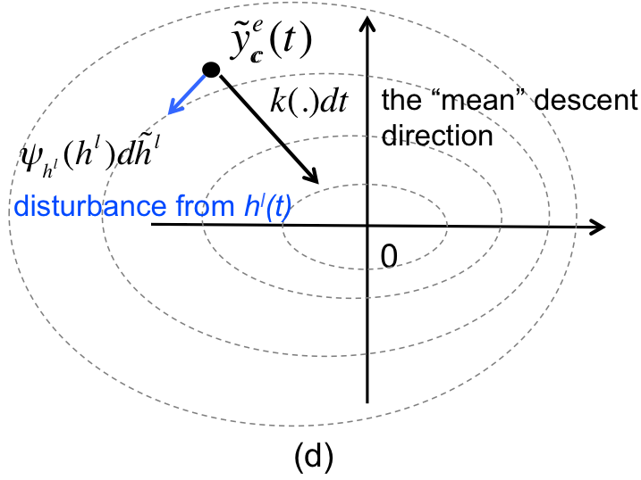
Figure 5: Illustrations of the convergence of the iterations $(x_{n_{s}},y_{n_{f}})$ and the virtual error dynamic systems $\widetilde{x}_{c}^{e}(t)$ and $\widetilde{y}_{c}^{e}(t)$. (a) The algorithm iteration $x_{n_{s}}$ tracks the target $\hat{x}(y(t),h(t))$, which is moving due to the time-varying $y(t)$ and $h(t)$. (b) The corresponding error state $\widetilde{x}_{c}^{e}(t)$ approaches to $0$ under the mapping $G(\centerdot)$. However, the exogenous disturbance $\widetilde{G}_{x}^{-1}\widetilde{G}_{h^{s}}(\centerdot)d\widetilde{h}^{s}$ and $\widetilde{G}_{x}^{-1}\widetilde{G}_{y}(\centerdot)dy_{c}$ drag it away from the origin. (c) The algorithm iteration $y_{n_{f}}$ tracks $y^{*}(h^{l}(t))$ following the “mean”virtual trajectory $y_{c}(t)$. (d) The corresponding error state $\widetilde{y}_{c}^{e}(t)$ approaches to $0$ following the virtual direction $k(\centerdot)$. However, the exogenous disturbance $\psi_{h^{l}}(\widetilde{h}^{l})d\widetilde{h}^{l}$ drags it away from the origin.

Such observation motivates us to offset the exogenous disturbance to reduce the tracking error under time-varying $h^{s}(t)$ and $h^{l}(t)$. We start by introducing compensation terms to the MCTS (30)-(31) as follows,

$$dx_{c} = G(x_{c},y_{c},\widetilde{h}^{s},\widetilde{h}^{l})dt\underbrace{-\widehat{\widetilde{G}_{x}^{-1}\widetilde{G}_{h^{s}}}(\centerdot)d\widetilde{h}^{s}}_{\mbox{\scriptsize compensation for }\widetilde{h}^{s}(t)}\underbrace{-\widehat{\widetilde{G}_{x}^{-1}\widetilde{G}_{y}(\centerdot)}dy_{c}}_{\mbox{\scriptsize\ compensation for }y(t)}$$ (43)

$$dy_{c} = N_{s}^{-1}k(y_{c},\widetilde{h}^{l})dt\underbrace{+\widehat{\psi_{h^{l}}(\widetilde{h}^{l})}d\widetilde{h}^{l}}_{\mbox{\scriptsize\ compensation for }\widetilde{h}^{l}(t)}$$ (44)

where $-\widehat{\widetilde{G}_{x}^{-1}\widetilde{G}_{h^{s}}}(\centerdot)d\widetilde{h}^{s}$ and $-\widehat{\widetilde{G}_{x}^{-1}\widetilde{G}_{y}(\centerdot)}dy_{c}$ are compensation terms to offset the disturbance in (41), and $\widehat{\psi_{h^{l}}(\widetilde{h}^{l})}d\widetilde{h}^{l}$ is a compensation term to offset the disturbance in (42). Here, for a simple discussion, we drop the reflection terms $dZ_{x}$ and $dZ_{y}$, since the projections that drive the reflections are always conservative. As a result, the dynamic system in (41)-(42) becomes

$$d\widetilde{x}_{c}^{e} = G(x_{c},y_{c},\widetilde{h}^{s},\widetilde{h}^{l})dt+\left(\widetilde{G}_{x}^{-1}\widetilde{G}_{h^{s}}(\centerdot)-\widehat{\widetilde{G}_{x}^{-1}\widetilde{G}_{h^{s}}(\centerdot)}\right)d\widetilde{h}^{s}$$

$$\qquad+\left(\widetilde{G}_{x}^{-1}\widetilde{G}_{y}(\centerdot)-\widehat{\widetilde{G}_{x}^{-1}\widetilde{G}_{y}(\centerdot)}\right)dy_{c}$$

$$d\widetilde{y}_{c}^{e} = N_{s}^{-1}k(y_{c},\widetilde{h}^{l})dt+\left(\widehat{\psi_{h^{l}}(\widetilde{h}^{l})}-\psi_{h^{l}}(\widetilde{h}^{l})\right)d\widetilde{h}^{l}.$$ (46)

Define the disturbance components as $\varphi_{x}^{h}(\centerdot)\triangleq-\widetilde{G}_{x}^{-1}\widetilde{G}_{h^{s}}(\centerdot)$, $\varphi_{x}^{y}(\centerdot)\triangleq-\widetilde{G}_{x}^{-1}\widetilde{G}_{y}(\centerdot)$ and $\varphi_{y}^{h}(\centerdot)\triangleq\psi_{h^{l}}(\centerdot)$. Consider $\hat{\varphi}_{x}^{h}(x;\centerdot)$, $\hat{\varphi}_{x}^{y}(x;\centerdot)$ and $\hat{\varphi}_{y}^{h}(y;\centerdot)$ as the compensation estimators for the disturbance components $\varphi_{x}^{h}(\centerdot)$, $\varphi_{x}^{y}(\centerdot)$ and $\varphi_{y}^{h}(\centerdot)$. The corresponding compensated mixed timescale algorithm is given by,

$$x_{n_{s}} = \mathcal{P}_{\mathcal{X}}\bigg{[}x_{n_{s}-1}+\gamma G(x_{n_{s}-1},y_{n_{f}};h^{s}(n_{f}\tau),h^{l}(n_{f}\tau))$$

$$\qquad\qquad+\hat{\varphi}_{x}^{h}(x_{n_{s}-1};\centerdot)(\triangle h^{s})_{n_{s}}+\hat{\varphi}_{x}^{y}(x_{n-1};\centerdot)(\triangle y)_{n_{s}}\bigg{]}$$

$$y_{n_{f}} = \mathcal{P}_{\mathcal{Y}}\left[y_{n_{f}-1}+\gamma K(x_{n_{s}},y_{n_{f}-1};h^{s}(n_{f}\tau),h^{l}(n_{f}\tau))+\hat{\varphi}_{y}^{h}(y_{n_{f}-1};\centerdot)(\triangle h^{l})_{n_{f}}\right]$$ (48)

where $(\triangle h^{s})_{n_{s}}=h^{s}(\lfloor\frac{n_{s}}{N_{s}}\rfloor\tau)-h^{s}(\lfloor\frac{n_{s}-1}{N_{s}}\rfloor\tau)$, $(\triangle y)_{n_{s}}=y_{\lfloor\frac{n_{s}}{N_{s}}\rfloor}-y_{\lfloor\frac{n_{s}-1}{N_{s}}\rfloor}$, and $(\triangle h^{l})_{n_{f}}=h^{l}(n_{f}\tau)-h^{l}(n_{f}\tau-\tau)$. The compensation terms are non-zero on the frame boundary.

V-B Derivation of the Compensation Estimators

Obviously, if we can precisely estimate the disturbance, its impact to the convergence can be totally suppressed and the tracking errors $\widetilde{x}_{c}^{e}$ and $\widetilde{y}_{c}^{e}$ go to zero. Unfortunately, we cannot obtain perfect estimations of the disturbance terms $-\widetilde{G}_{x}^{-1}\widetilde{G}_{h^{s}}(\centerdot)$, $-\widetilde{G}_{x}^{-1}\widetilde{G}_{y}(\centerdot)$, and $\psi_{h^{l}}(h^{l})$, because they require closed form expressions of the target $(\hat{x}(y,h^{s},h^{l}),y^{*}(h^{l}))$. In this section, we derive approximate compensation terms using Lagrange duality theory [32, 33] and implicit function theorem in calculus.

V-B1 Compensation for the Short-term Iteration $x_{n_{s}}$

Consider the optimality condition [33] for the inner problem (7),

$$\mathcal{G}(\theta_{x},\lambda_{x};\theta_{y},h^{s},h^{l})=\left[\begin{array}[]{c}\nabla_{x}F(\theta_{x},\theta_{y};h^{s},h^{l})-\sum_{i}\lambda_{x,i}\nabla w_{i}(\theta_{x},\theta_{y};\centerdot)\\ \{\lambda_{x,i}w_{i}(\theta_{x},\theta_{y};\centerdot)\}_{i=1}^{W}\end{array}\right]=0$$

where $\lambda_{x,i}\geq 0$ and $w_{i}(\theta_{x},\theta_{y};\centerdot)\leq 0$, for all $1\leq i\leq W$. From the Lagrangian duality theory, $\mathcal{G}(x;\theta_{y},h^{s},h^{l})=0$ has a unique solution $\hat{x}=(\hat{\theta}_{x},\hat{\lambda}_{x})$ for $\hat{\lambda}_{x}\geq 0$, and the dynamics of $\hat{x}(t)$ should satisfy $\mathcal{G}_{x}(\hat{x};\centerdot)\frac{d\hat{x}}{dt}+\mathcal{G}_{h^{s}}(\hat{x};\centerdot)\frac{dh^{s}}{dt}+\mathcal{G}_{y}(\hat{x};\centerdot)\frac{dy_{c}}{dt}=0$. Suppose the matrix $\mathcal{G}_{x}(x;\centerdot)$ is invertible. Using the implicit function theorem, the compensation estimators can be given by

$$\hat{\varphi}_{x}^{h}(x;\centerdot)=-\mathcal{G}_{x}^{-1}\mathcal{G}_{h^{s}}(x;\centerdot),\;\mbox{and}\;\hat{\varphi}_{x}^{y}(x;\centerdot)=-\mathcal{G}_{x}^{-1}\mathcal{G}_{y}(x;\centerdot).$$ (49)

V-B2 Compensation for the Long-term Iteration $y_{n}$

From the Lagrange duality theory, the optimality condition for the outer problem (10) is given by

$$\mathcal{T}(\theta_{y},\lambda_{y};h^{l})=\left[\begin{array}[]{c}\nabla_{y}\mathbb{E}F(\theta_{x},\theta_{y};h^{s},h^{l})-\sum_{j}\lambda_{y,j}\nabla q_{j}(\theta_{y};h^{l})\\ \{\lambda_{y,j}q_{j}(\theta_{y};h^{l})\}_{j=1}^{J}\end{array}\right]=0$$ (50)

where $\lambda_{y,j}\geq 0$ and $q_{j}(\theta_{y};\centerdot)\leq 0$, for all $1\leq j\leq J$. Similarly, $\mathcal{T}(y;\centerdot)=0$ has a unique solution $y^{*}=(\theta_{y}^{*},\lambda_{y}^{*})$ for $\lambda_{y}^{*}\geq 0$, and the dynamics of $y^{*}(t)$ should satisfy $\mathcal{T}_{y}(y^{*};\centerdot)\frac{dy^{*}}{dt}+\mathcal{T}_{h^{l}}(y^{*};\centerdot)\frac{dh^{l}}{dt}=0$. Also, using implicit function theorem, an ideal compensation estimator can be given by $-\mathcal{T}_{y}^{-1}\mathcal{T}_{h^{l}}(y;\centerdot)$.

Note that closed form expression is usually not available for $\mathcal{T}(y;\centerdot)$, due to the expectation $\mathbb{E}F(\centerdot)$. Alternatively, define $\hat{\mathcal{T}}(\theta_{y},\lambda_{y};h^{s},h^{l})\triangleq\left[\begin{array}[]{c}\nabla_{y}F(\theta_{x},\theta_{y};h^{s},h^{l})-\sum_{j}\lambda_{y,j}\nabla q_{j}(\theta_{y};\centerdot)\\ \{\lambda_{y,j}q_{j}(\theta_{y};\centerdot)\}_{j=1}^{J}\end{array}\right]$. Then for given $h^{l}$, $\hat{\mathcal{T}}_{y}(y;\centerdot)$ is an unbiased estimator of $\mathcal{T}_{y}(y;\centerdot)$, since $\mathbb{E}\hat{\mathcal{T}}(y;\centerdot)=\mathcal{T}(y;\centerdot)$. Similarly, $\hat{\mathcal{T}}_{h^{l}}(y;\centerdot)$ is a unbiased estimator of $\mathcal{T}_{h^{l}}(y;\centerdot)$. As a result, the compensation estimator for the long-term iteration can be given by

$$\hat{\varphi}_{y}^{h}(y;\centerdot)=-\hat{\mathcal{T}}_{y}^{-1}\mathcal{\hat{T}}_{h^{l}}(y;\centerdot).$$ (51)

V-C Performance of the Compensation Algorithm

Although the compensation estimators derived in (49) and (51) are from approximation, we can show that under some technical conditions, the tracking errors $\widetilde{x}_{c}^{e}$ and $\widetilde{y}_{c}^{e}$ from continuous-time trajectories $x_{c}(t)$ and $y_{c}(t)$ can be significantly eliminated.

Theorem 6 (Tracking performance of the compensation algorithm)

Assume CSI timescale separation for $h^{l}(t)$ and $h^{s}(t)$, i.e., $\epsilon\ll a_{H}$. Suppose that $\hat{\varphi}_{x}^{h}(\centerdot)$, $\hat{\varphi}_{x}^{y}(\centerdot)$ and $\hat{\varphi}_{y}^{h}(y;\centerdot)$ take the forms in (49) and (51), and they are Lipschitz continuous, i.e., there exist positive constants $\hat{L}_{x}^{h},\hat{L}_{x}^{y},\hat{L}_{y}^{h},\beta_{y}^{h}<\infty$, such that $\|\hat{\varphi}^{h}(x;\centerdot)-\hat{\varphi}^{h}(\hat{x};\centerdot)\|\leq\hat{L}_{x}^{h}\|x-\hat{x}\|$, $\|\hat{\varphi}^{y}(x;\centerdot)-\hat{\varphi}^{y}(\hat{x};\centerdot)\|\leq\hat{L}_{x}^{y}\|x-\hat{x}\|$ and $\mathbb{E}\|\hat{\varphi}_{y}^{h}(y;\centerdot)-\varphi_{y}^{h}(\centerdot)\|\leq\hat{L}_{y}^{h}\|y-y^{*}\|+\beta_{y}^{h}$, for all $x\in\mathcal{X}(y)$, $y\in\mathcal{Y}$. Then, if

(i) $$\alpha_{y}\gamma-\epsilon\tau\hat{L}_{y}^{h}>0,\;\mbox{and}$$

(ii) $$\alpha_{x}-\frac{a_{H}\tau}{\sqrt{2\pi}N_{s}\gamma}\hat{L}_{x}^{h}-\hat{L}_{x}^{y}N_{s}^{-1}l_{y}\frac{\epsilon\tau\beta_{y}^{h}}{\alpha_{y}\gamma-\epsilon\tau\hat{L}_{y}^{h}}-\frac{a_{H}\tau}{N_{s}\gamma}\left(\hat{L}_{x}^{h}\right)^{2}>0,$$

the tracking error $\widetilde{x}_{c}^{e}$ converges to $0$ in probability, and the the tracking error for $\widetilde{y}_{c}^{e}$ is upper bounded by $\mathbb{E}\|\widetilde{y}_{c}^{e}\|\leq\frac{\epsilon\tau\beta_{y}^{h}}{\alpha_{y}\gamma-\epsilon\tau\hat{L}_{y}^{h}}$.   ∎

Proof:

Please refer to Appendix G for the proof. ∎

In the case when $h^{l}$ is static, the convergence result is given in the following corollary.

Corollary 3 (Tracking performance under static $h^{l}$)

Suppose $\hat{\varphi}_{x}^{h}(\centerdot)$ and $\hat{\varphi}_{x}^{y}(\centerdot)$ are given by (49) and Lipschitz continuous as specified in Theorem 6. Then if $\alpha_{x}-\frac{a_{H}\tau}{\sqrt{2\pi}N_{s}\gamma}\hat{L}_{x}^{h}-\hat{L}_{x}^{y}N_{s}^{-1}l_{y}\frac{\epsilon\tau\beta_{y}^{h}}{\alpha_{y}\gamma-\epsilon\tau\hat{L}_{y}^{h}}-\frac{a_{H}\tau}{N_{s}\gamma}\left(\hat{L}_{x}^{h}\right)^{2}>0$, the tracking error $\widetilde{x}_{c}^{e}$ converges to $0$ in probability.   ∎

Corollary 3 is obtained by setting the timescale parameter $\epsilon=0$ in Theorem 6. It corresponds to the case 1 scenario studied in Section III-A. However, the performance with compensation is stronger because it does not require the short-term CSI timescale to be extremely slower than the algorithm timescale (i.e., $a_{H}\tau\ll\gamma$) in Theorem 2 and Corollary 1 for the convergence.

Remark 4 (Interpretation of the results)

Theorem 6 and Corollary 3 show the performance advantage of the compensation algorithm under time-varying CSI. Specifically, we have the following observations.

• Compensation for the long-term control: When the bias $\beta_{y}^{h}$ of the compensation estimator goes to $0$, the tracking error $\widetilde{y}_{c}^{e}=y_{c}-y^{*}$ of the long-term variable $y$ converges to $0$ as well. Note that the bias $\beta_{y}^{h}$ comes from using $\nabla_{y}F(\centerdot)$ to estimate $\nabla_{y}\mathbb{E}F(\centerdot)$ in (50). To reduce the bias, we can use a Monte-Carlo method to estimate $\widehat{\nabla_{y}\mathbb{E}F(\centerdot)}=\frac{1}{M}\sum_{m=1}^{M}\nabla_{y}F(x_{m},y_{0})$, by observing many realizations of $\nabla_{y}F(x(t),y(t_{0});\centerdot)$ in the inner timescale.

• Compensation for the short-term control: Theorem 6 implies that when the short timescale CSI $h^{s}(t)$ does not change too fast (moderate $a_{H}$), the compensation algorithm can keep track with the stationary point target. This is a much weaker condition for the conventional convergence result, which requires $a_{H}\tau\ll\gamma$, i.e., the algorithm must iterate much faster than the CSI dynamics. Moreover, one can reduce the frame duration $\tau$, increase the number of slots $N_{s}$ per frame, or increase the step size $\gamma$ to satisfy condition (ii) for enhancing the tracking of the inner iteration $x_{n_{s}}$, at the cost of larger signaling overhead, higher computational complexity and larger steady state error $\mathcal{O}(\gamma)$ as discussed in Section IV-B.

∎

Note that, even though there can be zero convergence errors for $x_{c}$ and $y_{c}$ in (43) and (44), the discrete-time iterations (V-A) and (48) still have $\mathcal{O}(\gamma)$ steady state error due to the constant step size $\gamma$ used for the tracking. Nevertheless, Theorem 6 and Corollary 3 indicate that the proposed compensation algorithm has an eminent convergence capability under time-varying $h^{s}(t)$ and $h^{l}(t)$.

VI An Application Example: Resource Allocations in Wireless Multi-hop Relay Network

The mixed timescale optimization approach has vast applications in wireless communication networks. In the following, we consider a particular example of joint flow control and power allocation in wireless relay network described in Section II-B. From this example, we demonstrate the compensation algorithm and apply the theoretical results for the convergence analysis.

VI-A The Two-Timescale Algorithm

We apply the stochastic primal-dual method in (26) to derive the iterative algorithm $x_{n_{s}}$ and $y_{n_{f}}$ in this example. Denote $x=(\mathbf{p},\lambda)$, where $\lambda=(\lambda_{1},\dots,\lambda_{W})$ is the Lagrange multiplier. For the example problem in (13), we can form the Lagrange function as

$$L(\mathbf{p},\lambda,\mathbf{r};\mathbf{h})=\sum_{j\in\mathcal{E}}\log(r_{j})-V\sum_{k\in\mathcal{L}}p_{k}-\sum_{j=1}^{J}\lambda_{j}\left[\sum_{k\in\mathcal{S}_{j}}c_{k}(\mathbf{r})-\log\left(1+\sum_{k\in\mathcal{S}_{j}}|h_{k}|^{2}p_{k}\right)\right]$$ (52)

where $W$ is the total number of constraints, and $\mathcal{S}_{j}\subset\mathcal{L}^{+}(m)$ for some $m\in\mathcal{R}\cup\{0\}$.

VI-A1 Iteration for the short-term variable

The optimality condition (KKT condition [41]) for the inner problem is given by

$$\mathcal{G}(\mathbf{p},\lambda;\mathbf{r},\mathbf{h})=\left[\begin{array}[]{c}\frac{\partial}{\partial\mathbf{p}}L(\mathbf{p},\lambda,\mathbf{r})\\ \left\{\lambda_{j}\left[\sum_{k\in\mathcal{S}_{j}}c_{k}(\mathbf{r})-\log\left(1+\sum_{k\in\mathcal{S}_{j}}|h_{k}|^{2}p_{k}\right)\right]\right\}_{j=1}^{W}\end{array}\right]=\mathbf{0}.$$

Following the adaptive compensation algorithm in Section V, the iteration of the short-term variable is given by

$$\mathbf{p}(n_{s}+1)=\mathcal{P}_{\mathbf{p}}\left[\mathbf{p}(n_{s})+\gamma\frac{\partial}{\partial\mathbf{p}}L\left(\mathbf{p}(n_{s}),\lambda(n_{s});\mathbf{r}(n_{f})\right)+\hat{\Psi}_{p}(\centerdot)\right]$$ (53)

$$\lambda(n_{s}+1)=\mathcal{P}_{\lambda}\left[\lambda(n_{s})-\gamma\frac{\partial}{\partial\lambda}L\left(\mathbf{p}(n_{s}),\lambda(n_{s});\mathbf{r}(n_{f})\right)+\hat{\Psi}_{\lambda}(\centerdot)\right]$$ (54)

where the projection $\mathcal{P}_{\mathbf{p}}\left(\centerdot\right)$ and $\mathcal{P}_{\lambda}\left(\centerdot\right)$ are to restrict the elements to be non-negative. The term $(\frac{\partial}{\partial\mathbf{p}}L(\centerdot),\frac{\partial}{\partial\lambda}L(\centerdot))$ corresponds to the iteration mapping $G(\centerdot)$ in (21) (and (V-A)). The compensations $\hat{\Psi}_{p}(\centerdot)$ and $\hat{\Psi}_{\lambda}(\centerdot)$ can be derived as

$$\left(\begin{array}[]{c}\hat{\Psi}_{p}(\centerdot)\\ \hat{\Psi}_{\lambda}(\centerdot)\end{array}\right)=-\mathcal{G}_{(\mathbf{p},\lambda)}^{-1}\mathcal{G}_{\mathbf{h}}(\mathbf{p}(n_{s}),\centerdot)\triangle\mathbf{h}(n_{s})-\mathcal{G}_{(\mathbf{p},\lambda)}^{-1}\mathcal{G}_{y}((\mathbf{p}(n_{s}),\centerdot)\triangle\mathbf{r}(n_{s})$$

where $\triangle\mathbf{h}(n_{s})=\mathbf{h}(\lfloor\frac{n_{s}}{N_{s}}\rfloor\tau)-\mathbf{h}(\lfloor\frac{n_{s}-1}{N_{s}}\rfloor\tau)$ and $\triangle\mathbf{r}(n_{s})=\mathbf{r}(\lfloor\frac{n_{s}}{N_{s}}\rfloor)-\mathbf{r}(\lfloor\frac{n_{s}-1}{N_{s}}\rfloor)$.

VI-A2 Iteration for the long-term variable

We first derive an augmented Lagrange function $L_{1}(\centerdot)$ by substituting the equality constraints (20) into the Lagrangian $L(\centerdot)$ in (52). The optimality condition for the outer problem is given by

$$\mathcal{T}(\mathbf{r};\mathbf{h}^{l})=\frac{\partial}{\partial\mathbf{r}}\mathbb{E}L_{1}(\mathbf{p}(n_{s}),\lambda(n_{s}),\mathbf{r}(n_{f}))=0.$$

The update of the long-term variable is given by

$$\mathbf{r}(n_{f}+1)=\mathcal{P}_{\mathbf{r}}\left[\mathbf{r}(n_{f})+\gamma\frac{\partial}{\partial\mathbf{r}}L_{1}\left(\mathbf{p}(n_{s}),\lambda(n_{s}),\mathbf{r}(n_{f})\right)+\hat{\Psi}_{r}(\centerdot)\right]$$ (55)

where the projection $\mathcal{P}_{\mathbf{r}}\left(\centerdot\right)$ is to restrict $\mathbf{r}$ to be non-negative. The iteration (55) corresponds to the long-term variable update for $y_{n_{f}}$ in (22), and the term $\frac{\partial}{\partial\mathbf{r}}L_{1}\left(\mathbf{p}(n_{s});\lambda(n_{s}),\mathbf{r}(n_{f})\right)$ corresponds to the stochastic estimator $K(\centerdot)$ in (22). The compensation $\hat{\Psi}_{r}(\centerdot)$ can be derived as

$$\hat{\Psi}_{r}(\mathbf{r}(n_{f}),\mathbf{h}^{l}(n_{f}\tau))=-\hat{\mathcal{T}}_{r}^{-1}\mathcal{\hat{T}}_{h^{l}}(\mathbf{r}(n_{f});\mathbf{h}^{l}(n_{f}))(\mathbf{h}^{l}(n_{f}\tau)-\mathbf{h}^{l}((n_{f}-1)\tau))$$

where $\hat{\mathcal{T}}(\mathbf{r};\mathbf{h}^{l})=\frac{\partial}{\partial\mathbf{r}}L_{1}(\mathbf{p},\lambda,\mathbf{r};\mathbf{h}^{l})$ and the path loss variable $\mathbf{h}^{l}(t)$ can be measured by averaging the CSI $\mathbf{h}(t)$ over a certain time window.

Table II summaries the algorithm association between the example and the mixed timescale model.

Components in the example		Corresponding components in the model
$(\mathbf{p}(n_{s}),\lambda(n_{s}))$	Primal-dual inner iteration (53)-(54)	$x_{n_{s}}$	Short-term iterative sequence (21)
$\mathbf{r}(n_{f})$	Primal outer iteration (55)	$y_{n_{f}}$	Long-term iterative sequence (22)
$(\hat{\Psi}_{p}(\centerdot),\hat{\Psi}_{\lambda}(\centerdot))$	Compensation for the inner iteration	$-\hat{\varphi}_{x}^{h}dh^{s}-\hat{\varphi}_{x}^{y}dy$	Compensation for the inner iteration
$\hat{\Psi}_{r}$	Compensation for the outer iteration	$\hat{\varphi}_{y}^{h}dh^{l}$	Compensation for the outer iteration
$\mathbb{R}_{+}^{|\mathcal{L}|}\times\mathbb{R}_{+}^{W}$	Projection domain for the inner iteration	$\mathcal{X}(y)$	Projection domain for $x_{n_{s}}$
$\mathbb{R}_{+}^{|\mathcal{L}|}$	Projection domain for the outer iteration	$\mathcal{Y}$	Projection domain for $y_{n_{f}}$

Table II: Algorithm associations between the example and the mixed timescale system model.

VI-B Implementation Considerations

With the iteration timescale decomposition, we can consider two implementation scenarios of the two-timescale algorithm: a) distributive implementation, and b) hybrid implementation.

Under distributive implementation, at each frame, each BS and RS node $m\in\mathcal{R}\cup\{0\}$ acquires the local CSI $\{h_{j}\}_{j\in\mathcal{L}^{+}(m)}$ and exchange the local control variables $\{p_{j}\}_{j\in\mathcal{L}^{+}(m)}$, $\{\lambda_{i}^{(m)}\}$ and $\{r_{j}\}_{j\in\mathcal{L}^{+}(m)}$ with neighbor nodes. It then updates the long-term flow control $\{r_{j}\}_{j\in\mathcal{L}^{+}(m)}$ once according to the outer iteration (55), and updates the power control variables $\{p_{j}\}_{j\in\mathcal{L}^{+}(m)}$ and $\{\lambda_{i}^{(m)}\}$ in each time slot according to the inner iterations (53) and (54). As an illustrative example, Fig. 6. a) demonstrates the message passing under distributive implementation and the network topology in Fig. 1.

Under hybrid implementation, there is a RRM server coordinating the message passing and the outer loop iterations in the network as illustrated in Fig. 1.. At the beginning of each frame, each BS and RS node $m\in\mathcal{R}\cup\{0\}$ obtains long-term flow control $\{r_{j}\}_{j\in\mathcal{L}^{+}(m)}$ from the RRM server and acquires the local CSI $\{h_{j}\}_{j\in\mathcal{L}^{+}(m)}$. It then updates the local power control variables $\{p_{j}\}_{j\in\mathcal{L}^{+}(m)}$ and $\{\lambda_{i}^{(m)}\}$ according to the inner iterations (53) and (54) in each time slot within the frame. At the end of the frame, it passes the local variables $\{p_{j}\}$ and $\{\lambda_{i}^{(m)}\}$ together with the local CSI $\{h_{j}\}$ for $j\in\mathcal{L}^{+}(m)$ to the RRM server. By collecting the short term variables $\mathbf{p}$ and $\lambda$ as well as the global CSI $\mathbf{h}$, the RRM server updates the long-term flow control $\mathbf{r}$ using the outer iteration (55) and feeds back to the BS and RSs at the beginning of the next frame. Fig. 6.b) illustrates the message passing under hybrid implementation and the network topology in Fig. 1.

Note that as the inner iterations (53) and (54) require only local CSI, they can be iterated for a finite number of steps $N_{s}>1$ at each frame to catch up with the fast timescale CSI variations. On the other hand, since the outer iteration (55) requires global coordination which involves signaling latency, it can only be updated once at each frame. However, as the long term flow control $\mathbf{r}$ adapts to CSI statistics (i.e., the long term CSI $\mathbf{h}^{l}$), it does not require a fast iteration and is not sensitive to signaling latency.

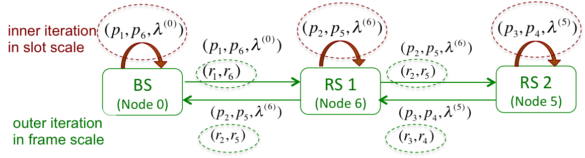
(a) Distributive implementation

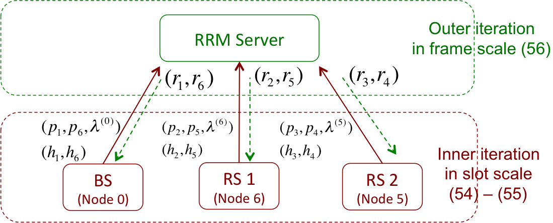
(b) Hybrid implementation

Figure 6: Example algorithm implementations and message passing for the network topology in Fig. 1.

Considering the computational complexity, the two-timescale algorithm with variable partitions reduces the computational cost at the central controller by distributing the computation of the cross-layer network utility optimization to different nodes locally. Table III gives a comparison on the computational complexity in terms of CPU time over one frame under the example in Section II-B. The inner iteration is assumed to update for $N_{s}=30$ steps in each frame under two-timescale algorithms. The one-timescale centralized algorithm consumes more CPU time, which may not be a good choice, since the transmission power control is delay-sensitive.

	RRM Server (ms)	Each BS (RS) (ms)
Two-timescale distributive algorithm	-	0.601
Two-timescale hybrid algorithm	0.0511	0.533
One-timescale centralized algorithm	1.26	-

Table III: Computational complexity in terms of CPU time of the one-timescale centralized algorithm and two-timescale algorithms over one frame. The simulation was done on a MATLAB platform running on a desktop computer with a 2.8 GHz single core CPU.

VI-C The Convergence Analysis

In this subsection, we derive the upper bound of the tracking error of the two-timescale iterations (53)-(55) using the theoretical results developed in Section III. We derive the convergence rate parameters $\alpha_{x}$ and $\alpha_{y}$ as follows.

Theorem 7 (Local convergence speed)

Denote

$$M_{L}(\centerdot)=\left(\begin{array}[]{cc}\frac{\partial^{2}}{\partial\mathbf{p}\partial\mathbf{p}}L(\centerdot)&\frac{\partial^{2}}{\partial\mathbf{p}\partial\lambda}L(\centerdot)\\ -\frac{\partial^{2}}{\partial\lambda\partial\mathbf{p}}L(\centerdot)&\mathbf{0}_{J\times J}\end{array}\right).$$

Then $M_{L}(\centerdot)$ is negative definite for all $(\mathbf{p}^{*},\mathbf{r}^{*})$ and $\lambda^{*}(\mathbf{p}^{*})$, under all $\mathbf{h}$. In addition, given any optimal points $\mathbf{w}=(\mathbf{p}^{*},\mathbf{r}^{*})$, we have the local convergence rate $\alpha_{x}(\mathbf{w})\geq-\lambda_{\max}(\frac{1}{2}(M_{L}(\mathbf{w})+M_{L}^{T}(\mathbf{w})))$, $\alpha_{y}(\mathbf{w})=-\lambda_{\max}\left(\frac{\partial^{2}}{\partial\mathbf{r}\partial\mathbf{r}}L(\mathbf{w})\right)$, where $\lambda_{\max}(A)$ denotes the maximum eigenvalue of matrix $A$.   ∎

Proof:

Please refer to Appendix H for the proof. ∎

Using Theorem 7, a lower bound of the global convergence rate can be obtained by $\alpha_{x}=\inf\{\alpha_{x}(\mathbf{\bm{\omega}}):\bm{\omega}\in\mathcal{X}(y)\times\mathcal{Y},\forall y\in\mathcal{Y},\forall\mathbf{h}\}$ and $\alpha_{y}=\inf\{\alpha_{y}(\bm{\omega}):\bm{\omega}\in\mathcal{X}(y)\times\mathcal{Y},\forall y\in\mathcal{Y},\forall\mathbf{h}\}$.

Given the results in Theorem 7, the the condition for algorithm stability and tracking error bound then directly follows from the results in Theorem 4 and 5, respectively.

Note that we can always enhance the convergence and increase $\alpha_{x}$ and $\alpha_{y}$ by introducing a carefully chosen positive definite scaling matrix $\Gamma$ in the iterations. However, the computation of the scaling matrix may increase the complexity for the inner iteration and require additional signaling overhead for the outer iteration.

VII Numerical Results

In this section, we simulate the tracking performance of the mixed timescale algorithm for the example cross-layer stochastic optimization problem studied in Section II-B and Section VI. We demonstrate the performance advantage of the mixed timescale algorithm over one-timescale algorithms under the CSI model discussed in Section II-A2. In addition, we show that the proposed two-timescale compensation algorithm in Section V significantly reduces the tracking error under time-varying CSI.

We consider the wireless heterogeneous relay network described in Section II-B. Specifically, the network has $1$ macro BS, $2$ RSs and $4$ mobile users who want to transmit data flows to the macro BS. The BSs are static and the mobiles are moving around with a speed at most $v_{\max}=100$ km/h. The mobility is according to the Levy walk mobility model in Section II-A1 with parameter $D_{\min}=75$ m, $\iota=1.8$ and $c_{0}=D_{\min}^{\iota}$. There are $6$ wireless links as illustrated in Fig. 1, and it is assumed that the network topology does not change during the simulation. Correspondingly, the long-term CSI timescale parameter is $\epsilon=6\times 10^{-4}$ sec^-1. The control objective is to determine the flow rate congestion control $\mathbf{r}$ and power allocation $\mathbf{p}$ according to the proportional fair utility in (13). The frame duration is $\tau=1$ ms, and the inner iterations (53) and (54) are updated for $N_{s}=30$ steps in each frame.

We consider the following baseline schemes:

• Baseline 1 - One-timescale centralized algorithm based on real-time global CSI [12, 1]: The central controller (RRM server in Fig. 1) solves the deterministic version (dropping the expectation) of the problem (13) at each time slot. The controller collects real-time global CSI (GCSI) $\mathbf{h}(t)$ at each time slot and computes the optimal flow rate congestion control $\mathbf{r}(\mathbf{h}(t))$ and power allocation $\mathbf{p}(\mathbf{h}(t))$ that adapt to each realization of $\mathbf{h}(t)$.

• Baseline 2 - One-timescale centralized algorithm based on statistical CSI [15]: For every $T_{s}=100$ ms, the central controller solves a relaxed version of the stochastic optimization problem (13), where the link capacity constraint (14) is replaced by the probability outage constraint $\mbox{Pr}\left[\eqref{eq:ex-constraint-capacity}\mbox{ is not satisfied}\right]\leq\Theta_{\text{out}}$, and the flow rate congestion control $\mathbf{r}$ and power allocation $\mathbf{p}$ adapt to the statistics of the GCSI $\mathbf{h}(t)$.

• Baseline 3 - Two-timescale stochastic gradient without compensations: The algorithm iterations are based on stochastic gradient in (23) and (24) in solving Problem 4.

Note that the baseline 1 suffers from huge computational complexity, as it searches for the optimal solution at each time slot, which is not scalable to large networks. Moreover, baseline 1 is very sensitive to signaling latency for the message passing throughout the network. On the other hand, baseline 2 is not sensitive to the signaling latency but it is too conservative as it does not exploit the local real-time CSI knowledge at the BS and the RSs. Hence, baseline 1 and baseline 2 are for performance benchmark only.

VII-A Performance of the Mixed Timescale Algorithms

Due to the exogenous stochastic variation of $h^{s}(t)$ and $h^{l}(t)$, the instantaneous link capacity constraint in (14) and (15) may not be satisfied for every iteration outputs. To quantify the associated performance penalty, we define the constraint outage probability as follows

$$\mathbb{P}_{\text{out}}=\frac{1}{N_{T}}\sum_{n=1}^{N_{T}}\sum_{j\in\mathcal{L}}1\left\{r_{j}\notin\mathcal{C}_{m}^{\text{cap}}(\mathbf{p}(n),\mathbf{h}(n)),\forall m:j\in\mathcal{L}^{+}(m)\right\}$$

where $N_{T}$ is the total number of transmission frames, $1\{\centerdot\}$ is the indicator function, and $\mathcal{C}_{m}^{\text{cap}}(\mathbf{p},\mathbf{h})$ is the multi-access channel (MAC) capacity region at receiver node $m$, and is specified by (12).

Note that, $a_{H}=50$ corresponds to around $10$ ms channel coherence time [31] and $a_{H}=1$ yields over 200 ms channel coherence time. Fig. 7 shows the constraint outage probability under different CSI fading parameters $a_{H}$ and $\epsilon=6\times 10^{-4}$. The constraint outage probability increases when the channel is changing faster, but the proposed two-timescale compensation algorithm has the least constraint outage probability compared with other baselines under $5$ ms signaling latency and various channel fading rates.

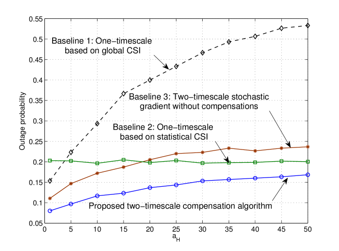
Figure 7: The constraint outage probability under different CSI fading parameters $a_{H}$ and $\epsilon=6\times 10^{-4}$. The signaling latency is $\tau=5$ ms.

Fig. 8.a) gives the throughput performance assuming no signaling latency. Baseline 1 yields the best performance, but it is highly sensitive to signaling latency, as shown in Fig. 8.b), where $5$ ms signaling latency is considered. In Fig. 8.b), as the CSI varies faster, the throughput performance of all the schemes decrease, except for baseline 2. However, baseline 2 does not exploit the short-term transmission opportunity and achieves only moderate performance. As a comparison, the proposed two timescale compensation algorithm has the best performance and is robust to signaling latency. Fig. 9 demonstrates the corresponding proportional fair utility for the different schemes under signaling latency of $5$ ms. The proposed algorithm performs much better than all the other schemes.

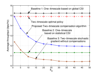
(a) Assuming no signaling latency

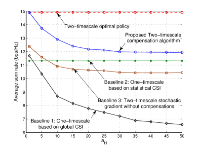
(b) $\tau=5$ ms signaling latency

Figure 8: Throughput performance of the different schemes under $\epsilon=6\times 10^{-4}$ and average SNR $11$ dB. Note that, $a_{H}=50$ corresponds to around $10$ ms channel coherence time [31] and $a_{H}=1$ yields over 200 ms channel coherence time.

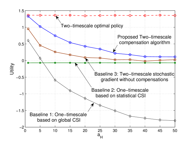
Figure 9: Proportional fair utility of the different schemes under 11 dB average SNR, $5$ ms signaling latency and the long timescale CSI parameter $\epsilon=6\times 10^{-4}$. The proposed algorithm performs much better than all the baseline schemes.

VII-B Tracking Performance of the Adaptive Compensation Algorithm

We evaluate the tracking performance of the two-timescale compensation algorithm over the baseline stochastic gradient algorithm.

Fig. 10 shows a snapshot of the algorithm trajectories of the proposed two-timescale compensation algorithm and the baseline stochastic gradient tracking algorithm without compensations, under short timescale CSI fading rate $a_{H}=10$ and long timescale parameter $\epsilon=6\times 10^{-4}$. The trajectories represent the online power allocation policy $p_{5}$. The proposed compensation algorithm quickly converges to the optimal trajectory of the inner iteration, while the baseline algorithm fails to track the optimal target and yields much larger tracking errors.

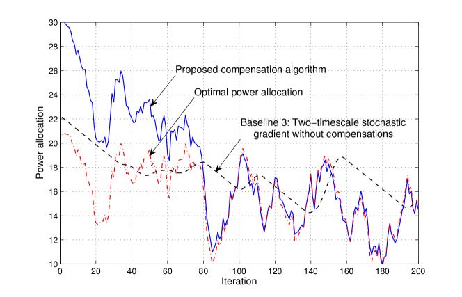
Figure 10: A snapshot of algorithm trajectories of the proposed compensation algorithm and the stochastic gradient algorithm without compensations under short timescale CSI fading parameter $a_{H}=10$ and long timescale parameter $\epsilon=6\times 10^{-4}$. The trajectories represent the online power allocation policy $p_{5}$. The proposed compensation algorithm quickly converges to the optimal trajectory of the inner iteration, while the baseline algorithm fails to track the optimal target and yields much larger tracking errors.

VIII Conclusions

In this paper, we have analyzed the convergence behavior of a mixed timescale cross-layer stochastic optimization driven by multi-timescale CSI. The CSI dynamic is modeled by an auto-regressive process in the short timescale (small-scale fading), and a mobility-driven dynamic process in the long timescale (large-scale fading). We partitioned the control variables into short-term control variables and long-term control variables, and studied the convergence of the corresponding mixed timescale stochastic iterative algorithm. We derived a VSDS and showed that studying the algorithm convergence is equivalent to studying the stochastic stability of the VSDS. Using Lyapunov stochastic stability analysis, we derived a sufficient condition for the algorithm to be stable. In addition, we derived a tracking error upper bound in terms of the parameters of the mixed timescale CSI process. Based on these results, we proposed an adaptive compensation algorithm for enhancing the tracking performance. The analysis framework and the proposed algorithms were applied to an application example in a wireless heterogeneous network. Numerical results matched with the theoretical insights and demonstrated significant performance gain of the proposed compensation algorithms over the baselines.

Appendix A Derivations of the Reflection Terms $z_{x}$ and $z_{y}$

Taking a small step $\triangle t$, the ODE dynamics (30)-(31) can be written as

$$x_{c}(t+\triangle t) = x_{c}(t)+G(x_{c}(t),y_{c}(t),h^{s}(t),h^{l}(t))\triangle t+z_{x}(t)\triangle t$$

$$= \mathcal{P}_{\mathcal{X}(y)}\left[x_{c}(t)+G(x_{c}(t),y_{c}(t),h^{s}(t),h^{l}(t))\triangle t\right]$$

$$y_{c}(t+\triangle t) = y_{c}(t)+k(y_{c}(t),h^{l}(t))\triangle t+z_{y}(t)\triangle t$$

$$= \mathcal{P}_{\mathcal{Y}}\left[y_{c}(t)+k(y_{c}(t),h^{l}(t))\triangle t\right].$$

Consider that the convex domains $\mathcal{X}(y)$ and $\mathcal{Y}$ can be specified by a set of constraints $\omega_{i}(x,y;h)\leq 0$, $i=1,\dots,W$, and $q_{i}(y;h^{l})\leq 0$, $i=1,\dots,J$, respectively. Then the Euclidean projections are equivalent to find the points $x_{0}(\triangle t)$ and $y_{0}(\triangle t)$, which solve the following minimization problems

$$\min_{x} \frac{1}{2}\|x-\left(x_{c}(t)+G(x_{c}(t),y_{c}(t),\centerdot)\triangle t\right)\|_{2}^{2}$$ (56)

subject to $$\omega_{i}(x,y;\centerdot)\leq 0,\qquad\forall i=1,\dots,W.$$

and

$$\min_{y} \frac{1}{2}\|y-\left(y_{c}(t)+k(y_{c}(t),\centerdot)\triangle t\right)\|_{2}^{2}$$ (57)

subject to $$q_{i}(y;\centerdot)\leq 0,\qquad\forall i=1,\dots,J.$$

The corresponding Lagrange functions are given by

$$L^{(x)}(x,y,\lambda_{x})=\frac{1}{2}\|x-\left[x_{c}(t)+G(\centerdot)\triangle t\right]\|_{2}^{2}+\sum_{i=1}^{W}\lambda_{x,i}=\omega_{i}(x,y;\centerdot)$$

and

$$L^{(y)}(y,\lambda_{y})=\frac{1}{2}\|y-\left[y_{c}(t)+k(\centerdot)\triangle t\right]\|_{2}^{2}+\sum_{i=1}^{J}\lambda_{y,i}q_{i}(y;\centerdot).$$

The KKT condition [32, 33] for the problem (56) on the $x$ variable is given by

$$x_{0}(\triangle t)-\left[x_{c}(t)+G(x_{c}(t),y_{c}(t),\centerdot)\triangle t\right]+\sum_{i=1}^{W}\lambda_{x,i}^{*}\nabla_{x}\omega_{i}(x_{0}(\triangle t),y_{c}(t);\centerdot) = 0$$ (58)

$$\lambda_{x,i}^{*}\omega_{i}(x_{0}(\triangle t),y_{c}(t);\centerdot) = 0,\;\forall i.$$ (59)

Solving (58)-(59), we obtain $x_{0}(\triangle t)$. Similarly, by writing the KKT condition for (57), we can obtain $y_{0}(\triangle t)$. Then the reflection terms are given by

$$z_{x}(t)=\lim_{\triangle t\to 0}\frac{x_{0}(\triangle t)-\left[x_{c}(t)+G(x_{c}(t),y_{c}(t),\centerdot)\triangle t\right]}{\triangle t}$$

and

$$z_{y}(t)=\lim_{\triangle t\to 0}\frac{y_{0}(\triangle t)-\left[y_{c}(t)+k(y_{c}(t),\centerdot)\triangle t\right]}{\triangle t}.$$

Appendix B Sketch Proof of Theorem 2

We ignore the transient states for $x_{n_{s}}$ and $y_{n_{f}}$, and just focus on their stationary states.

For the inner iteration $x_{n_{s}}$ in (21), consider a large enough $n_{s}$. Since $\mu_{n_{f}}$ is decreasing, we have $\mu_{n_{f}}\ll\gamma$. From the timescale condition $a_{H}\tau\ll\gamma$ and the step size condition $\mu_{n_{f}}\ll\gamma$, the iteration (21) finds the partial optimum $\hat{x}(y,h(n_{f}\tau))$ for each $h(t)=(h_{1}(t),\dots,h_{N}(t))$, where $h_{j}(t)=h_{j}^{l}h_{j}^{s}(t)$. This can be shown under Assumption 3 and 4 given a sufficiently small step size $\gamma$ [32, 33]. Note that the partial stationary point $\hat{x}(y,h(n_{f}\tau))$ of (21) is also the partial equilibrium point $x_{c}(t)$ of (30). Therefore, we have established that $x_{n_{s}(t)}\to x_{c}(t)$, where $n_{s}(t)=\lfloor tN_{s}/\tau\rfloor$.

For the outer iteration $y_{n_{f}}$ in (22), with sufficient large $n_{f}$, we have

$$\mathbb{E}\left[K(x_{n_{s}-1},y_{n_{f}-1};h^{s}(n_{f}\tau),h^{l}\big{|}h^{l}\right] = \mathbb{E}\left[\Gamma_{y}\nabla_{y}F(\hat{x}(y_{n_{f}-1},\centerdot),y_{n_{f}-1};h^{s}(n_{f}\tau),h^{l})\big{|}h^{l}\right]$$ (60)

$$= \mathbb{E}\left[\Gamma_{y}\nabla_{y}\mathcal{P}_{1}(y,h^{s},h^{l})\big{|}h^{l}\right]$$

$$= \Gamma_{y}\int\nabla_{y}\mathcal{P}_{1}(y,\omega,h^{l})dF_{h^{s}}(\omega)$$

$$= \Gamma_{y}\nabla_{y}\int\mathcal{P}_{1}(y,\omega,h^{l})dF_{h^{s}}(\omega)$$

$$= \Gamma_{y}\nabla_{y}\mathbb{E}\left[\mathcal{P}_{1}(y,h^{s},h^{l})\big{|}h^{l}\right]$$

$$\triangleq \overline{K}(y,h^{l})$$

where $F_{h^{s}}(\omega)$ is the cumulative distribution function of the conditional probability $\mbox{Pr}(h^{s}=\omega\big{|}h^{l})=\mbox{Pr}(h^{s}=\omega)$, and the interchange of the integration and the differentiation is because the integration is bounded (i.e., the expectation of $F(\centerdot)$ is bounded). We take conditional expectation here because $y$ adapts to each realization of $h^{l}$. Therefore, we have the gradient estimator $K(\centerdot)=\overline{K}(y,h^{l})+\xi(\centerdot)$, where $\xi(\centerdot)$ is some “noise” and $\mathbb{E}\xi(\centerdot)=0$. Using the stochastic approximation [36, 19], $y_{n}$ converges to $y^{*}$ almost surely under the assumed step size rule for $\mu_{n}$.

From Assumption 4, the matrix $\nabla_{y}k(y,h^{l})=\nabla_{y}\mathbb{E}[K(\centerdot)]=\mathbb{E}\left[\nabla_{y}K(\centerdot)\right]$ is a negative definite matrix. Therefore, the system $\dot{y}_{c}=\nabla_{y}k(y_{c},h^{l})$ is asymptotically stable [39] at a unique stationary point $y_{c}^{*}(h^{l})$, where $\dot{y}_{c}^{*}(h^{l})=\nabla_{y}k(y_{c},h^{l})=0$. According to the definition of $k(y,h^{l})$, we have $\overline{K}(y,h^{l})\equiv k(y,h^{l})$. This implies that the stationary point $y_{n}$ of (22) is just the equilibrium $y_{c}^{*}$ of (31), i.e., $y^{*}=y_{c}^{*}$. Then we have established the asymptotic result for $\lim\sup_{t\to\infty}\mbox{Pr}\left\{\|y_{n_{f}(t)}-y_{c}(t)\|>\eta\right\}=0$, where $n_{f}(t)=\lfloor t/\tau\rfloor$.

Appendix C Proof of Lemma 1

The above results are obtained from the implicit function theorem. From the optimality condition $\widetilde{G}(\hat{x}_{c},y_{c},h^{s},h^{l})=0$ and the implicit function theorem, we have

$$d\hat{x}_{c}(y_{c},\centerdot) = \widetilde{G}_{x}^{-1}(\hat{x}_{c}(y_{c},\centerdot),y_{c},h^{s},h^{l})\bigg{[}\widetilde{G}_{h^{s}}(\hat{x}_{c}(y_{c},\centerdot),y_{c},h^{s},h^{l})dh^{s}$$

$$\qquad\qquad+\widetilde{G}_{h^{l}}(\hat{x}_{c}(y_{c},\centerdot),y_{c},h^{s},h^{l})dh^{l}+\widetilde{G}_{y}(\hat{x}_{c}(y_{c},\centerdot),y,h^{s},h^{l})dy\bigg{]}.$$

But since $dh^{l}\ll dh^{s}$ due to the small variation of $h^{l}(t)$ (controlled by $\epsilon\ll a_{H}$), the term $G_{h^{l}}(\centerdot)dh^{l}$ is comparatively small. Ignoring this term, equation (33) yields.

Appendix D Proof of Theorem 3

Theorem 3 can be obtained from the weak convergence results in [36, 19, 43]. In the following, we sketch briefly how we can apply those results.

Recall that the algorithm is implemented on the timescale $t_{n_{f}}=n_{f}\tau$, where $n_{f}$ is the frame index and $\tau$ is the frame duration. To establish the VSDS, we define the virtual algorithm timescales as follows.

Definition 11 (Virtual algorithm timescale)

The virtual algorithm timescale on frame is a mapping from the frame index $n_{f}$ to a real number $s_{n_{f}}=n_{f}N_{s}\gamma$. The virtual algorithm timescale on slot is a mapping from the slot index $n_{s}$ to a real number $\widetilde{s}_{n_{s}}=n_{s}\gamma$.   ∎

Under the virtual algorithm timescale, the iteration indices are related as $n_{s}(s)=\lfloor s/\gamma\rfloor$ and $n_{f}(s)=\lfloor s/(N_{s}\gamma)\rfloor$. The virtual algorithm times is just a scaled implementation time, and their relationship is given by $t_{n_{f}}=N_{s}n_{f}\gamma\frac{\tau}{N_{s}\gamma}=s_{n_{f}}\frac{\tau}{N_{s}\gamma}$.

Accordingly, denote the virtual CSI state as $\widetilde{h}^{s}(s)$. Since $dt_{n_{f}}=\frac{\tau}{N_{s}\gamma}ds_{n_{f}}$, the timescale of the virtual CSI dynamics $\widetilde{h}^{s}(s)$ can be aligned with the virtual algorithm timescale $s_{n_{f}}$ by adding a gain parameter $\frac{\tau}{N_{s}\gamma}$ to (1) as,

$$d\widetilde{h}^{s}=-\frac{1}{2}\frac{a_{H}\tau}{N_{s}\gamma}\widetilde{h}^{s}ds+\sqrt{\frac{a_{H}\tau}{N_{s}\gamma}}dW_{s}.$$ (61)

$\widetilde{h}^{s}(s)$ has the same shape as $h^{s}(t)$, but with a different timescale.

The same trick applies to the long-term virtual CSI dynamics $\widetilde{h}^{l}(s)$, as $d\widetilde{h}_{j}^{l}=-\frac{\tau}{N_{s}\gamma}c_{0}\iota D_{j}(s)^{-\iota-1}v_{j}(s)ds$, $\forall j$. In a vector form, we have

$$d\widetilde{h}^{l}=-\frac{\tau}{N_{s}\gamma}H_{L}(t)ds$$ (62)

where $H_{L}(t)$ is an $N\times N$ diagonal matrix, with the $j$-th diagonal element being $c_{0}\iota D_{j}(t)^{-\iota-1}v_{j}(t)$. The virtual CSI timescale separation parameter becomes $\widetilde{\epsilon}=\frac{\tau}{N_{s}\gamma}\epsilon$.

We use a localization method [43] and consider the algorithm trajectories (21)-(22) and (30)-(31) start from $(x_{0},y_{0})$ at time $s=s_{0}=0$, which lies in the neighborhood of $(x^{*}(\widetilde{h}^{s},\widetilde{h}^{l}),y^{*}(\widetilde{h}^{l}))$. We have

$$x_{n_{s}}-x_{c}(\widetilde{s}_{n_{s}})$$ (64)

$$= x_{n_{s}-1}-x_{c}(\widetilde{s}_{n_{s}-1})$$

$$\quad+\gamma\bigg{[}G(x_{n_{s}-1},y_{n_{f}},\widetilde{h}^{s}(s_{n_{f}}),\widetilde{h}^{l}(s_{n_{f}}))+z_{x,n_{s}}-G(x_{c}(\widetilde{s}_{n_{s}-1}),y_{c}(s_{n_{f}}),\widetilde{h}^{s}(s_{n_{f}}),\widetilde{h}^{l}(s_{n_{f}}))-z_{x}(\widetilde{s}_{n_{s}})\bigg{]}$$

$$\quad-\left[x_{c}(\widetilde{s}_{n_{s}})-x_{c}(\widetilde{s}_{n_{s}-1})-\gamma G(x_{c}(\widetilde{s}_{n_{s}-1}),y_{c}(s_{n_{f}}),\widetilde{h}^{s}(s_{n_{f}}),\widetilde{h}^{l}(s_{n_{f}}))-z_{x}(\widetilde{s}_{n_{s}})\right]$$

where using Taylor expansion,

$$\mbox{term }\eqref{eq:app-weak-conv-xn-1} = \gamma G_{x}\left(x_{c}(\widetilde{s}_{n_{s}-1}),y_{c}(s_{n_{f}}),\widetilde{h}^{s}(s_{n_{f}}),\widetilde{h}^{l}(s_{n_{f}})\right)\left(x_{n_{s}-1}-x_{c}(\widetilde{s}_{n_{s}-1})\right)$$

$$\qquad\qquad-\gamma G_{y}\left(x_{c}(\widetilde{s}_{n_{s}-1}),y_{c}(s_{n_{f}}),\widetilde{h}^{s}(s_{n_{f}}),\widetilde{h}^{l}(s_{n_{f}})\right)\left(y_{n_{f}}-y_{c}(s_{n_{f}})\right)+o(\gamma).$$

Here, it is reasonable to consider $z_{x,n_{s}}-z_{x}(\widetilde{s}_{n_{s}})=0$, since if the partial equilibrium $\hat{x}_{c}\in\mathring{\mathcal{X}}$, we eventually have $z_{x,n_{s}}=z_{x}(\widetilde{s}_{n_{s}})=0$. If $\hat{x}_{c}\in\partial\mathcal{X}$, both trajectories eventually search along the boundary, and $z_{x,n_{s}}=z_{x}(\widetilde{s}_{n_{s}})$ for a large enough $n_{s}$.

The term (64) is just a first order Taylor expansion of the continuous trajectory (30) at the point $x_{c}(\widetilde{s}_{n_{s}-1})$. By taking $\widetilde{x}_{c}^{\gamma}(\widetilde{s}_{n_{s}})=\frac{1}{\sqrt{\gamma}}\left(x_{n_{s}}-x_{c}(\widetilde{s}_{n_{s}})\right)$ and $\widetilde{y}_{c}^{\gamma}(s_{n_{f}})=\frac{1}{\sqrt{\gamma}}\left(y_{n_{f}}-y_{c}(s_{n_{f}})\right)$, we have

$$\widetilde{x}_{c}^{\gamma}(\widetilde{s}_{n}) = \widetilde{x}_{c}^{\gamma}(0)+\gamma\sum_{j=0}^{n-1}\bigg{[}G_{x}\left(x_{c}(\widetilde{s}_{j}),y_{c}(s_{\underline{j}}),\widetilde{h}^{s}(s_{\underline{j}}),\widetilde{h}^{l}(s_{\underline{j}})\right)\widetilde{x}_{c}^{\gamma}(\widetilde{s}_{j})$$

$$\qquad\qquad\qquad+G_{y}\left(x_{c}(\widetilde{s}_{j}),y_{c}(s_{\underline{j}}),\widetilde{h}^{s}(s_{\underline{j}}),\widetilde{h}^{l}(s_{\underline{j}})\right)\widetilde{y}_{c}^{\gamma}(s_{\underline{j}})\bigg{]}+o(\gamma)$$

$$= \widetilde{x}_{c}^{\gamma}(0)+\int_{0}^{\widetilde{s}_{n}}\left(G_{x}(\centerdot)\widetilde{x}_{c}^{\gamma}+G_{y}(\centerdot)\widetilde{y}_{c}^{\gamma}\right)ds+o(\gamma)$$

where $\underline{j}\triangleq\lfloor j/N_{s}\rfloor$ frame index of the outer iteration when the inner iteration is at the $j$-th slot. Equivalently,

$$d\widetilde{x}_{c}^{\gamma}=G_{x}(\centerdot)\widetilde{x}_{c}^{\gamma}ds+G_{y}(\centerdot)\widetilde{y}_{c}^{\gamma}ds+o(\gamma).$$ (65)

Similarly, we derive the dynamic $\widetilde{y}_{c}^{\gamma}(s)$ as follows.

$$y_{n_{f}}-y_{c}(s_{n_{f}})$$ (68)

$$= y_{n_{f}-1}-y_{c}(s_{n_{f}-1})$$

$$\quad+N_{s}\gamma\left[N_{s}^{-1}K\left(x_{\overline{n_{f}}},y_{n_{f}-1};\centerdot\right)+z_{y,n_{f}}-N_{s}^{-1}K\left(\hat{x}_{c}(s_{n_{f}-1}),y_{c}(s_{n_{f}-1});\centerdot\right)-\hat{z}_{y}(s_{n_{f}})\right]$$

$$\quad+\gamma\left[K\left(\hat{x}_{c}(s_{n_{f}-1}),y_{c}(s_{n_{f}-1});\centerdot\right)+\hat{z}_{y}(s_{n_{f}})-k(y_{c}(s_{n_{f}-1}),\widetilde{h}^{l}(s_{n_{f}}))-z_{y}(s_{n_{f}})\right]$$

$$\quad-\left[y_{c}(s_{n_{f}})-y_{c}(s_{n_{f}-1})-\gamma k(y_{c}(s_{n_{f}-1}),\widetilde{h}^{l}(s_{n_{f}}))-\gamma z_{y}(s_{n_{f}})\right]$$

where $\overline{n_{f}}\triangleq N_{s}n_{f}$ is the slot index of the inner iteration when the outer iteration is at the $n_{f}$-th frame . The
$\mbox{term }\eqref{eq:app-weak-conv-yn-1}$

$$= (N_{s}\gamma)N_{s}^{-1}\bigg{[}K\left(x_{\overline{n_{f}}},y_{n_{f}-1};\centerdot\right)-K\left(\hat{x}_{c}(s_{n_{f}-1}),y_{n_{f}-1};\centerdot\right)$$

$$\qquad\qquad+K\left(\hat{x}_{c}(s_{n_{f}-1}),y_{n_{f}-1};\centerdot\right)-K\left(\hat{x}_{c}(s_{n_{f}-1}),y_{c}(s_{n_{f}-1});\centerdot\right)\bigg{]}$$

$$= (N_{s}\gamma)N_{s}^{-1}K_{x}\left(\hat{x}_{c}(s_{n_{f}-1}),y_{c}(s_{n_{f}-1});\centerdot\right)\left(x_{\overline{n_{f}}-1}-x_{c}(s_{n_{f}-1})+x_{c}(s_{n_{f}-1})-\hat{x}_{c}(s_{n_{f}-1})\right)$$

$$\qquad\qquad+(N_{s}\gamma)N_{s}^{-1}K_{y}\left(\hat{x}(s_{n_{f}-1}),y_{c}(s_{n_{f}-1});\centerdot\right)(y_{n_{f}-1}-y_{c}(s_{n_{f}-1}))+o(\gamma)$$

$$= (N_{s}\gamma)N_{s}^{-1}K_{x}\left(\hat{x}_{c}(s_{n_{f}-1}),y_{c}(s_{n_{f}-1});\centerdot\right)\left(\widetilde{x}_{c}^{\gamma}+\widetilde{x}_{c}^{e,\gamma}\right)$$

$$\qquad\qquad+(N_{s}\gamma)N_{s}^{-1}K_{y}\left(\hat{x}_{c}(s_{n_{f}-1}),y_{c}(s_{n_{f}-1});\centerdot\right)\widetilde{y}_{c}^{\gamma}+o(\gamma)$$

by the first order Taylor expansion of function $K(\centerdot)$ at $(\hat{x}_{c}(s_{n_{f}-1}),y_{c}(s_{n_{f}-1}))$. Note that, since $\triangle s=s_{n_{f}}-s_{n_{f}-1}=N_{s}\gamma$,

$$\frac{1}{\sqrt{\gamma}}\mbox{term }\eqref{eq:app-weak-conv-yn-1}=N_{s}^{-1}K_{x}(\hat{x}_{c},y_{c},\centerdot)(\widetilde{x}_{c}^{\gamma}+\widetilde{x}_{c}^{e,\gamma})\triangle s+N_{s}^{-1}K_{y}(\hat{x}_{c},y_{c},\centerdot)\widetilde{y}_{c}^{\gamma}\triangle s+o(\gamma).$$ (69)

Consider $y^{*}(\widetilde{h}^{l})\in\mathring{\mathcal{Y}}$ is in the interior of the domain. (The case when $y^{*}(\widetilde{h}^{l})$ is on the boundary will be discussed later). Then it is reasonable to consider $y_{n_{f}}\in\mathring{\mathcal{Y}}$, with probability 1. We consider the following process for the term (68),

$$S^{\gamma}(s):=\gamma\sum_{j=1}^{n_{f}(s)}\left[K(\hat{x}_{c}(s_{j}),y_{c}(s_{j});\centerdot)-k(y_{c}(s_{j});\widetilde{h}^{l})\right].$$

Choosing a sufficiently small $\delta>0$, we have

$$S^{\gamma}(s+\delta)-S^{\gamma}(s)\approx\gamma\sum_{j=n_{f}(s)+1}^{n_{f}(s+\delta)}\left[K(\hat{x}_{c}(s_{j}),y;\centerdot)-k(y;\widetilde{h}^{l})\right].$$

where $y=y_{c}(s)$. The above is an approximation since we use $y_{c}(s_{j})\approx y_{c}(s)$ for $n_{f}(s)<j\leq n_{f}(s+\delta)$. However, the approximation is asymptotically accurate for sufficiently small $\delta$ and $\gamma$. The central limit theorem for the state dependent process suggests that $\hat{\Sigma}_{s,\delta}^{-1/2}\left(S^{\gamma}(s+\delta)-S^{\gamma}(s)\right)$ weakly converge to a normal random variable, where $\hat{\Sigma}_{s,\delta}$ is the covariance matrix of $S^{\gamma}(s+\delta)-S^{\gamma}(s)$ [36]. This implies that

$$\frac{1}{\sqrt{\gamma}}\left(S^{\gamma}(s+\delta)-S^{\gamma}(s)\right)\to\int_{s}^{s+\delta}\widetilde{\Sigma}_{s,\delta}^{\frac{1}{2}}dW_{u}$$ (70)

where $W_{u}$ is a standard Winner process and

$$\widetilde{\Sigma}(y_{c}(s_{0});\widetilde{h}^{l}) = \gamma\sum_{j=-\infty}^{+\infty}\mbox{cov}\left[K\left(\hat{x}_{c}(s_{j}),y_{c}(s_{j});\widetilde{h}(s_{j})\right),K\left(\hat{x}_{c}(s_{0}),y_{c}(s_{0});\widetilde{h}(s_{0})\right)\big{|}\widetilde{h}^{l}\right]$$

is the covariance matrix of the estimator $K(\centerdot)$ under the virtual long-term CSI state $\widetilde{h}^{l}$. In addition, we have

$$\hat{\Sigma}(y_{c};\widetilde{h}^{l}) \triangleq \sum_{j=-\infty}^{+\infty}\mbox{cov}\left[K\left(\hat{x}_{c}(t_{j}),y_{c}(t_{j});h(t_{j})\right),K\left(\hat{x}_{c}(t_{0}),y_{c}(t_{0});h(t_{0})\right)\big{|}\widetilde{h}^{l}\right]$$

$$= \frac{N_{s}}{\tau}\widetilde{\Sigma}(y_{c};\widetilde{h}^{l})$$

to be the covariance matrix of the estimator $K(\centerdot)$ under the CSI state $h$, since the virtual algorithm timescale $s_{n}$ is $\frac{\tau}{N_{s}\gamma}$ times denser than the implementation timescale $t_{n}$. Therefore, from (69) and (70), we obtain

$$d\widetilde{y}_{c}^{\gamma}=N_{s}^{-1}K_{x}(\hat{x}_{c},y_{c},\centerdot)(\widetilde{x}_{c}^{\gamma}+\widetilde{x}_{c}^{e,\gamma})ds+N_{s}^{-1}K_{y}(\hat{x}_{c},y_{c},\centerdot)\widetilde{y}_{c}^{\gamma}ds+\frac{\tau}{N_{s}}\hat{\Sigma}^{\frac{1}{2}}(y_{c};\widetilde{h}^{l})dW_{s}+o(\gamma).$$

Note that, in a finite horizon case for $s\in[0,T_{s}]$, by letting $\gamma\to 0$, one can drop the $o(\gamma)$ term and obtain the convergence results $(\widetilde{x}_{c}^{\gamma},\widetilde{y}_{c}^{\gamma})\to(\widetilde{x}_{c},\widetilde{y}_{c})$, where $(\widetilde{x}_{c},\widetilde{y}_{c})$ is the solution to (71)-(D). In addition, using the sophisticated techniques in [36, 19], one can further prove the convergence in the infinite horizon case for $s\in[0,\infty)$ and obtain the following,

$$d\widetilde{x}_{c} = G_{x}(x_{c},y_{c},\widetilde{h}^{s},\widetilde{h}^{l})\widetilde{x}_{c}ds+G_{y}(x_{c},y_{c},\widetilde{h}^{s},\widetilde{h}^{l})\widetilde{y}_{c}ds$$ (71)

$$d\widetilde{y}_{c} = N_{s}^{-1}K_{x}(\hat{x}_{c},y_{c},\centerdot)(\widetilde{x}_{c}+\widetilde{x}_{c}^{e})ds+N_{s}^{-1}K_{y}(\hat{x}_{c},y_{c},\centerdot)\widetilde{y}_{c}ds$$

$$\qquad+\sqrt{\tau N_{s}^{-1}}\Sigma^{\frac{1}{2}}(y_{c},\widetilde{h}^{l})dW_{s}+dZ_{y}.$$

where $\Sigma^{\frac{1}{2}}(y_{c},\widetilde{h}^{l})=\hat{\Sigma}^{\frac{1}{2}}(y_{c},\widetilde{h}^{l})$ in the case for $y^{*}(\widetilde{h}^{l})\in\mathring{\mathcal{Y}}$.

Moreover, changing the MCTS (30)-(31) into to the virtual algorithm time $s$, we get

$$dx_{c} = G(x_{c},y_{c,}\widetilde{h}^{s},\widetilde{h}^{l})ds+dZ_{x}$$ (73)

$$dy_{c} = N_{s}^{-1}k(y_{c},\widetilde{h}^{l})ds+dZ_{y}$$ (74)

where $dZ_{x}$ and $dZ_{y}$ are reflection terms. Notice that $d\widetilde{x}_{c}^{e}=dx_{c}-d\hat{x}_{c}$ and $d\widetilde{y}_{c}^{e}=dy_{c}-dy^{*}$. We obtain the following error dynamic system

$$d\widetilde{x}_{c}^{e} = G(x_{c},y_{c},\widetilde{h}^{s},\widetilde{h}^{l})ds+dZ_{x}+\widetilde{G}_{x}^{-1}\widetilde{G}_{h^{s}}(\centerdot)d\widetilde{h}^{s}+\widetilde{G}_{x}^{-1}\widetilde{G}_{y}(\centerdot)dy_{c}$$ (75)

$$d\widetilde{y}_{c}^{e} = N_{s}^{-1}k(y_{c},\widetilde{h}^{l})ds+dZ_{y}-\psi_{h^{l}}(\widetilde{h}^{l})d\widetilde{h}^{l}$$ (76)

Consider the SDEs (71)-(D) and (75)-(76), and the virtual CSI dynamics (61)-(62). Rearranging the terms and changing the virtual time notation $s$ to $t$, we obtain the VSDS in (37). This proves the claimed results.

Remark 5 (The case $y^{*}(\widetilde{h}^{l})$ on the boundary)

When $y^{*}(\widetilde{h}^{l})$ is on the boundary, we can follow the argument in [43] to find out the behavior of $\widetilde{y}_{c}(s)$. Note that the corresponding effect is only on the diffusion term $\Sigma^{\frac{1}{2}}(y_{c},\widetilde{h}^{l})dW_{s}$, where $\Sigma(y_{c},\widetilde{h}^{l})=\Sigma_{0}(y_{c})\hat{\Sigma}(y_{c},\widetilde{h}^{l})$, and $\Sigma_{0}(y)=\mbox{diag}\left(\{\sigma_{i}^{0}(y)\}_{i=1}^{N_{y}}\right)$, which is defined in the following. Consider the $i$-th component of $y^{*}(\widetilde{h}^{l})$ is on the boundary. There are two cases. Case i), the $i$-th component of the drift $k(y^{*};h^{l})$ is non-zero, which means there must be a reflection force $z_{y}^{(i)}\neq 0$ on $y_{n_{f}}^{(i)}$ and $y_{c}^{(i)}$ to keep them from reaching out of the boundary. Then obviously, upon reaching $y^{*(i)}$, $y_{n_{f}}^{(i)}$ is not likely to be disturbed by the noise from the estimator $K(\centerdot)$ [unless the noise is larger than the drift $k^{(i)}(y^{*};h^{l})$], and the $i$-th component of the diffusion term $\Sigma^{\frac{1}{2}}(y_{c},\widetilde{h}^{l})dW_{s}$ should be zero. Hence $\sigma_{i}^{0}=0$. Case ii), the $i$-th component of the drift $k(y^{*};h^{l})$ is zero, which means the reflection force $z_{y}^{(i)}$ depends on the disturbance noise. According to [43], we can simply consider $\sigma_{i}^{0}=1$, just as the case when $y^{*}(\widetilde{h}^{l})$ is in the interior of $\mathcal{Y}$.   ∎

Appendix E Proof of Theorem 4

E-A The Lyapunov Drift of the VSDS

It is equivalent to show the VSDS $u(t)$ is stochastically stable. We first give the following lemma.

Lemma 3 (Ito’s lemma)

Consider a stochastic process $u(t)$ given by the following SDE, $du=f(u)dt+g(u)dW_{t}$ and a function $V(u)\in\mathbb{R}_{+}$. The Lyapunov drift operator on $V(\centerdot)$ can be written as $\widetilde{\mathcal{L}}V=\frac{\partial V}{\partial u}f(u)+\mbox{tr}\left[g(u)^{T}\frac{\partial^{2}V}{\partial uu^{T}}g(u)\right].$   ∎

We first consider that the optimal solution $y^{*}$ is in the interior of $\mathcal{Y}$, which means the reflection term $dZ_{y}\equiv 0$ and the matrix $\Sigma^{0}$ (defined in Appendix D) is an identity matrix. Then using Lemma 9, the Lyapunov drift of the stochastic process $u(t)$ can be written as

$$\widetilde{\mathcal{L}}V(u) = \left[\begin{array}[]{c}\widetilde{x}_{c}\\ \widetilde{y}_{c}\end{array}\right]^{T}\left[\begin{array}[]{cc}G_{x}(x_{c},y_{c},\centerdot)&G_{y}(x_{c},y_{c},\centerdot)\\ N_{s}^{-1}K_{x}(\hat{x}_{c},y_{c},\centerdot)&N_{s}^{-1}K_{y}(\hat{x}_{c},y_{c},\centerdot)\end{array}\right]\left[\begin{array}[]{c}\widetilde{x}_{c}\\ \widetilde{y}_{c}\end{array}\right]$$

$$\qquad+\widetilde{y}_{c}^{T}N_{s}^{-1}K_{x}(\hat{x}_{c},y_{c},\centerdot)\widetilde{x}_{c}^{e}+\left(\widetilde{x}_{c}^{e}\right)^{T}G(x_{c},\centerdot)+\left(\widetilde{x}_{c}^{e}\right)^{T}G_{x}^{-1}G_{h^{s}}(-\frac{1}{2})\frac{a_{H}\tau}{N_{s}\gamma}\widetilde{h}^{s}$$

$$\qquad+\left(\widetilde{x}_{c}^{e}\right)^{T}G_{x}^{-1}G_{y}N_{s}^{-1}k(y_{c},\widetilde{h}^{l})+\left(\widetilde{y}_{c}^{e}\right)^{T}N_{s}^{-1}k(y_{c},\widetilde{h}^{l})$$

$$\qquad+\frac{\tau}{N_{s}\gamma}\left(\widetilde{y}_{c}^{e}\right)^{T}\psi_{h^{l}}(\widetilde{h}^{l})H_{L}-\frac{1}{2}\frac{a_{H}\tau}{N_{s}\gamma}\left(\widetilde{h}^{s}\right)^{T}\widetilde{h}^{s}+\frac{1}{2}\mbox{tr}\left(\tau N_{s}^{-1}\Sigma(y_{c})\right)$$

$$\qquad+\frac{1}{2}\mbox{tr}\left[\frac{a_{H}\tau}{N_{s}\gamma}\left(G_{x}^{-1}G_{h^{s}}\right)^{T}\left(G_{x}^{-1}G_{h^{s}}\right)+\frac{a_{H}\tau}{N_{s}\gamma}\mathbf{I}\right]$$

where $\hat{x}_{c}$ denotes the partial optimum $\hat{x}_{c}(y_{c},h^{s},h^{l};t)$.

E-B The Upper Bound of the Drift

We bound each term from the above equation in the following.

First of all, from Assumption 4, we can show that

$$Q_{c} \triangleq [\begin{array}[]{cc}\widetilde{x}_{c}^{T}&\widetilde{y}_{c}^{T}\end{array}]\left[\begin{array}[]{cc}G_{x}(x_{c},y_{c},h)&G_{y}(x_{c},y_{c}h)\\ N_{s}^{-1}K_{x}(x_{c},y_{c},h)&N_{s}^{-1}K_{y}(x_{c},y_{c},h)\end{array}\right]\left[\begin{array}[]{c}\widetilde{x}_{c}\\ \widetilde{y}_{c}\end{array}\right]$$ (89)

$$\leq -N_{s}^{-1}\alpha(\|\widetilde{x}_{c}\|^{2}+\|\widetilde{y}_{c}\|^{2}).$$ (90)

Secondly, the mapping $G(x_{c},\centerdot)$ on the $x$ part has the property

$$(\widetilde{x}_{c}^{e})^{T}G(x_{c,}\centerdot) = (\widetilde{x}_{c}^{e})^{T}\int_{0}^{1}G_{x}(x_{c}^{*}+\xi\widetilde{x}_{c}^{e},\centerdot)\widetilde{x}_{c}^{e}d\xi$$ (91)

$$\leq -\alpha_{x}\|\widetilde{x}_{c}^{e}\|^{2}.$$

Thirdly, the mean mapping $k(y_{c},\widetilde{h}^{l})$ on the $y$ part satisfies

$$(\widetilde{y}_{c}^{e})^{T}k(y_{c},\widetilde{h}^{l}) = (\widetilde{y}_{c}^{e})^{T}\lim_{n\to\infty}\mathbb{E}\left[K(y_{c},\widetilde{h}^{l})\right]$$ (92)

$$= \lim_{n\to\infty}\mathbb{E}\left[(\widetilde{y}_{c}^{e})^{T}\int_{0}^{1}K_{y}(y_{c}^{*}+\xi\widetilde{y}_{c}^{e},\widetilde{h}^{l})\widetilde{y}_{c}^{e}d\xi\right]$$

$$\leq \lim_{n\to\infty}\mathbb{E}\left[\int_{0}^{1}-\alpha_{y}\|\widetilde{y}_{c}^{e}\|^{2}d\xi\right]$$

$$= -\alpha_{y}\|\widetilde{y}_{c}^{e}\|^{2}.$$

In addition, since $K(y^{*},\widetilde{h}^{l})=\mathbf{0}$ due to the property of the stationary point $y^{*}\in\mathring{\mathcal{Y}}$, we have

$$\|k(y_{c},\widetilde{h}^{l})\| = \lim_{n\to\infty}\mathbb{E}\|K(y_{c},\widetilde{h}^{l})\|$$ (93)

$$= \lim_{n\to\infty}\mathbb{E}\|K(y_{c},\widetilde{h}^{l})-K(y_{c}^{*},\widetilde{h}^{l})\|$$

$$\leq \lim_{n\to\infty}\mathbb{E}l_{y}\|y_{c}-y_{c}^{*}\|$$

$$= l_{y}\|\widetilde{y}_{c}^{e}\|$$

where the inequality is from the Lipschitz property in Assumption 4.

Finally, using the above result, we can find an upper bound for the Lyapunov drift in (E-A) as

$$\mathcal{\widetilde{\mathcal{L}}}V \leq -N_{s}^{-1}\alpha\left(\|\widetilde{x}_{c}\|^{2}+\|\widetilde{y}_{c}\|^{2}\right)+\frac{l_{x}}{N_{s}}\|\widetilde{y}_{c}\|\|\widetilde{x}_{c}^{e}\|-\alpha_{x}\|\widetilde{x}_{c}^{e}\|^{2}+\frac{1}{2}v_{H}\|\widetilde{x}_{c}^{e}\|\|\widetilde{h}^{s}\|\frac{a_{H}\tau}{N_{s}\gamma}$$

$$\qquad+\frac{v_{y}l_{y}}{N_{s}}\|\widetilde{x}_{c}^{e}\|\|\widetilde{y}_{c}^{e}\|-\frac{\alpha_{y}}{N_{s}}\|\widetilde{y}_{c}^{e}\|^{2}+\frac{\epsilon\tau}{N_{s}\gamma}\varpi\|\widetilde{y}_{c}^{e}\|-\frac{1}{2}\frac{a_{H}\tau}{N_{s}\gamma}\|\widetilde{h}^{s}\|^{2}+C_{0}(y^{*}(\widetilde{h}^{l}))$$

$$\triangleq \phi(\chi)$$ (95)

where $C_{0}(y^{*}(\widetilde{h}^{l}))=\frac{\tau}{2N_{s}}\mbox{tr}\left(\Sigma(y^{*})\right)+\frac{1}{2}\frac{a_{H}\tau}{N_{s}\gamma}v_{H}^{2}N+\frac{1}{2}\frac{a_{H}\tau}{N_{s}\gamma}N$ is from the trace terms in (E-A). The parameter $N$ is the dimension of the parameters $h^{s}$ and $h^{l}$. $\phi:\chi\mapsto\mathbb{R}$ is the upper bound drift function and $\chi=(\|\widetilde{x}_{c}\|,\|\widetilde{y}_{c}\|,\|\widetilde{x}_{c}^{e}\|,\|\widetilde{y}_{c}^{e}\|,\|\widetilde{h}^{s}\|)$ is the vector measuring the deviations of each virtual state from the origin.

Note that $\phi(\chi)$ is a quadratic function and we can write it as

$$\phi(\chi)=-\chi^{T}A\chi+b^{T}\chi+C_{0}$$

where

$$A=\left[\begin{array}[]{ccccc}\frac{\alpha}{N_{s}}&&&\dots&0\\ &\frac{\alpha}{N_{s}}&-\frac{l_{x}}{2N_{s}}&&\vdots\\ &-\frac{l_{x}}{2N_{s}}&\alpha_{x}&-\frac{v_{y}l_{y}}{2N_{s}}&-\frac{v_{H}a_{H}\tau}{4N_{s}\gamma}\\ \vdots&&-\frac{v_{y}l_{y}}{2N_{s}}&\frac{a_{y}}{N_{s}}&0\\ 0&\dots&-\frac{v_{H}a_{H}\tau}{4N_{s}\gamma}&0&\frac{1}{2}\frac{a_{H}\tau}{N_{s}\gamma}\end{array}\right]$$ (96)

$b=[0,0,0,\frac{\epsilon\varpi\tau}{N_{s}\gamma},0]^{T}$ and $C_{0}=\frac{1}{2N_{s}}\left[\tau\mbox{tr}\left(\Sigma(y^{*})\right)+\frac{a_{H}\tau}{\gamma}N(1+v_{H}^{2})\right]$.

According to Lemma 2, a sufficient condition for the VSDS $u(t)$ to be mean square stable is that the function $\widetilde{\mathcal{L}}V(u)\leq\phi(\chi)$ can be further upper bounded by $\phi(\chi)\leq-f(\chi)+C_{f}$, where $f(\chi)=c\chi^{T}\chi$, for some constant $c>0$ and $C_{f}<\infty$. This is equivalent to verifying if the function $\phi(\chi)+f(\chi)=-\chi^{T}(A-c\mathbf{I})\chi+b^{T}\chi+C_{0}$ is bounded above. Therefore, we only need to check the positive definite property of the coefficient matrix $A$. To do this, we can calculate each of the leading principle minors of $A$, and make them positive. These calculations lead to the sufficient condition (39) in Theorem 4.

Remark 6 (The case $y^{*}(\widetilde{h}^{l})$ on the boundary)

When the optimal solution $y^{*}$ is on the boundary of the constraint domain, we may have non-zero $dZ_{y}$ and a non-identity matrix $\Sigma_{0}(y_{c})$. We may have the following two modifications in the above flow. (i) The term $\widetilde{y}_{c}^{T}\left[K_{x}(\centerdot)\left(\widetilde{x}_{c}+\widetilde{x}_{c}^{e}\right)+K_{y}(\centerdot)\widetilde{y}_{c}\right]$ in (E-A) and (90) now becomes $\widetilde{y}_{c}^{T}\left[K_{x}(\centerdot)\left(\widetilde{x}_{c}+\widetilde{x}_{c}^{e}\right)+K_{y}(\centerdot)\widetilde{y}_{c}+dZ_{y}\right]$. Since the term about the $x$ variable $K_{x}(\centerdot)\left(\widetilde{x}_{c}+\widetilde{x}_{c}^{e}\right)$ does not contribute to the reflection $dZ_{y}$, we only need to evaluate $\widetilde{y}_{c}^{T}\left[K_{y}(\centerdot)\widetilde{y}_{c}+dZ_{y}\right]$. Note that, when there is a non-zero reflection on the $i$-th component of $y_{c}$, we must have $\widetilde{y}_{c}^{(i)}=0$ for most of the time. Thus we still have $\widetilde{y}_{c}^{T}\left[K_{y}(\centerdot)\widetilde{y}_{c}+dZ_{y}\right]\widetilde{y}_{c}\leq-\alpha_{y}\|\widetilde{y}_{c}\|^{2}$, as we did in (90). (ii) Consider the covariance matrix in (D). Its trace must be smaller than the case when $y^{*}(\widetilde{h}^{l})$ is in the interior, since there are some zero diagonal elements in the matrix $\Sigma_{0}(y^{*})$ [see Appendix D]. Thus the constant $C_{0}$ defined above is still an upper bound. Combining the cases (i) and (ii), the optimal solution $y^{*}$ being on the boundary does not change the upper bound of the drift as in (E-B).  ∎

Appendix F Proof of Theorem 5

Choose a function $f(\chi)=c\chi^{T}A\chi$ for some constant $0<c<1$. We have $f(\chi)\geq c\lambda_{\min}(A)\|\chi\|^{2}$, where $\lambda_{\min}(A)$ denotes the smallest eigenvalue of matrix $A$.

Under the sufficient condition in Theorem 4 and from (95), we have the stochastic Lyapunov drift be upper bounded by

$$\widetilde{\mathcal{L}}V(u)\leq\phi(\chi(u))=-\chi^{T}A\chi+b^{T}\chi+C_{0}\leq-f(\chi)+C_{1}$$

where $C_{1}=C_{0}+\frac{C_{b}}{1-c}$, and $C_{b}=\frac{1}{4}b^{T}A^{-1}b=\left(\frac{\epsilon\varpi\tau}{N_{s}\gamma}\right)^{2}\frac{4N_{s}^{-1}\alpha\alpha_{x}-N_{s}^{-2}l_{x}^{2}-N_{s}^{-2}l_{y}^{2}v_{y}^{2}}{N_{s}^{-1}\alpha(8\alpha_{x}-a_{H}v_{H}^{2})-2N_{s}^{-2}l_{x}^{2}-2N_{s}^{-2}l_{y}^{2}v_{y}^{2}}<\infty$.

Then, using Lemma 2, we have

$$\lim\sup_{t\to\infty}\frac{1}{t}\int_{0}^{t}\mathbb{E}\|u(\tau)\|^{2}d\tau \leq \frac{1}{c\lambda_{\min}(A)}\times\lim\sup_{t\to\infty}\frac{1}{t}\int_{0}^{t}\left(C_{0}+\frac{C_{b}}{1-c}\right)d\tau$$

$$= \frac{1}{c\lambda_{\min}(A)}\left(\overline{C}_{0}+\frac{C_{b}}{1-c}\right)$$

where $\overline{C}_{0}=\frac{1}{2N_{s}}\left[\tau\overline{\Sigma}+\frac{a_{H}\tau}{\gamma}N(1+v_{H}^{2})\right]$, and $\overline{\Sigma}=\lim\sup_{t\to\infty}\frac{1}{t}\int_{0}^{t}\mbox{tr}\left(\Sigma(y^{*}(h^{l}(\tau)))\right)d\tau$ is the time-averaged covariance matrix of the estimator $K(\centerdot)$. Choosing $c$ to minimize the above upper bound, we obtain $c^{*}=\frac{\overline{C}_{0}+C_{b}}{2\overline{C}_{0}}$. With the observation that $C_{b}(\epsilon^{2})$ can typically be very small, due to the small timescale separation parameter $\epsilon\ll 1$. Then we choose $c=\frac{1}{2}$ for a reasonable tight upper bound of the tracking error.

We now derive the term $\lambda_{\min}(A)$, by using the eigenvalue lower bound $\lambda_{\min}(A)\geq\frac{\left|\det\left(A\right)\right|}{2^{n/2-1}\|A\|_{F}}$ from [44], where $\|\centerdot\|_{F}$ denotes the Frobenius norm and $n$ is the dimension of $A$. We apply a trick to obtain a good eigenvalue bound by letting $A_{0}=N_{s}A$. Then $\lambda_{\min}(A)=N_{s}^{-1}\lambda_{\min}(A_{0})\geq N_{s}^{-1}\frac{\left|\det\left(A_{0}\right)\right|}{2^{3/2}\|A_{0}\|_{F}}=N_{s}^{-1}\frac{\rho}{\eta}$, where $\rho=\left|\det\left(A_{0}\right)\right|=\frac{\alpha a_{H}\tau}{16\gamma}\left(8N_{s}\alpha\alpha_{x}\alpha_{y}-\alpha\alpha_{y}\frac{a_{H}\tau}{\gamma}v_{H}^{2}-2\alpha_{y}l_{x}^{2}-2\alpha l_{y}^{2}v_{y}^{2}\right)=\mathcal{O}(N_{s}\alpha^{2}\alpha_{x}\alpha_{y})$ and $\eta=2^{3/2}\|A_{0}\|_{F}=\mathcal{O}\left(\sqrt{N_{s}^{2}\alpha_{x}^{2}+\alpha^{2}}\right)$ . Therefore, we have

$$\lim\sup_{t\to\infty}\frac{1}{t}\int_{0}^{t}\mathbb{E}\|u(\tau)\|^{2}d\tau \leq \frac{1}{\frac{1}{2}N_{s}^{-1}\frac{\rho}{\eta}}\left(\frac{1}{2N_{s}}\left[\tau\overline{\Sigma}+\frac{a_{H}\tau}{\gamma}N(1+v_{H}^{2})\right]+C_{b}(\epsilon^{2})\right)$$

$$= \frac{\eta}{\rho}\left(\tau\overline{\Sigma}+C\right)$$

where $C=\frac{a_{H}\tau}{\gamma}N(1+v_{H}^{2})+4C_{b}(\epsilon)=\frac{a_{H}\tau}{\gamma}N(1+v_{H}^{2})+\mathcal{O}(\epsilon^{2}\varpi^{2}\tau^{2}\gamma^{-2})$.

Since $\|\widetilde{x}_{c}\|^{2}+\|\widetilde{x}_{c}^{e}\|^{2}+\|\widetilde{y}_{c}\|^{2}+\|\widetilde{y}_{c}^{e}\|^{2}\leq\|u\|^{2}$, we have $e_{x}+e_{y}\leq\frac{\eta}{\rho}\left(\frac{1}{2}\overline{\Sigma}+C\right)$.

Appendix G Proof of Theorem 6

Using the compensated MCTS (43)-(44) and the CSI dynamics (1)-(2), the dynamic system (V-A)-(46) can be written as

$$d\widetilde{x}_{c}^{e} = G(x_{c,}y_{c};\centerdot)dt+\left(\varphi_{x}^{h}(\centerdot)-\hat{\varphi}_{x}^{h}(\centerdot)\right)(-\frac{a_{H}\tau}{2N_{s}\gamma}\widetilde{h}^{s})dt+\left(\varphi_{x}^{y}(\centerdot)-\hat{\varphi}_{x}^{y}(\centerdot)\right)N_{s}^{-1}k(y_{c},\widetilde{h}^{l})dt$$ (97)

$$\qquad+\left(\varphi_{x}^{y}(\centerdot)-\hat{\varphi}_{x}^{y}(\centerdot)\right)\hat{\varphi}_{y}^{h}(y_{c},\widetilde{h}^{s},\widetilde{h}^{l})d\widetilde{h}^{l}+\left(\varphi_{x}^{h}(\centerdot)-\hat{\varphi}_{x}^{h}(\centerdot)\right)\sqrt{\frac{a_{H}\tau}{N_{s}\gamma}}dW_{t}$$

$$d\widetilde{y}_{c}^{e} = N_{s}^{-1}k(y_{c},\widetilde{h}^{l})dt+\left(\varphi_{y}^{h}(\widetilde{h}^{l})-\hat{\varphi}_{y}^{h}(y_{c},\widetilde{h}^{s},\widetilde{h}^{l})\right)d\widetilde{h}^{l}$$ (98)

Consider two Lyapunov functions $V_{1}(\widetilde{x}_{c}^{e})=\frac{1}{2}\left(\widetilde{x}_{c}^{e}\right)^{T}\widetilde{x}_{c}^{e}$ and $V_{2}(\widetilde{y}_{c}^{e})=\frac{1}{2}(\widetilde{y}_{c}^{e})^{T}\widetilde{y}_{c}^{e}$ defined along the trajectory of the virtual system (97)-(98).

Define $\xi_{y}^{h}(y_{c},\widetilde{h}^{s},\widetilde{h}^{l})\triangleq\|\varphi_{y}^{h}(\widetilde{h}^{l})-\hat{\varphi}_{y}^{h}(y_{c},\widetilde{h}^{s},\widetilde{h}^{l})\|-\mathbb{E}\|\varphi_{y}^{h}(\widetilde{h}^{l})-\hat{\varphi}_{y}^{h}(y_{c},\widetilde{h}^{s},\widetilde{h}^{l})\|$. Note that $\xi_{y}^{h}(\centerdot)$ acts like a “noise” term that depends on $\widetilde{h}^{s}$ and satisfies $\mathbb{E}\xi_{y}^{h}(\centerdot)=0$. Using Lemma 3, the Lyapunov drift of $V_{2}(\centerdot)$ is given by

$$\widetilde{\mathcal{L}}V_{2}(\centerdot) = (\widetilde{y}_{c}^{e})^{T}N_{s}^{-1}k(y_{c},\widetilde{h}^{l})+(\widetilde{y}_{c}^{e})^{T}\left(\varphi_{y}^{h}(\widetilde{h}^{l})-\hat{\varphi}_{y}^{h}(y_{c},\widetilde{h}^{s},\widetilde{h}^{l})\right)\frac{d\widetilde{h}^{l}}{dt}$$ (99)

$$\leq -\frac{\alpha_{y}}{N_{s}}\|\widetilde{y}_{c}^{e}\|^{2}+\|\widetilde{y}_{c}^{e}\|\left(\hat{L}_{y}^{h}\|\widetilde{y}_{c}^{e}\|+\beta_{y}^{h}+\xi_{y}^{h}(\centerdot)\right)\frac{\tau}{N_{s}\gamma}\epsilon(D_{\min},v_{\max})$$

$$= -\left(\widetilde{\alpha}_{y}-\widetilde{\epsilon}\hat{L}_{y}^{h}\right)\|\widetilde{y}_{c}^{e}\|^{2}+\widetilde{\epsilon}\beta_{y}^{h}\|\widetilde{y}_{c}^{e}\|+\widetilde{\epsilon}\xi_{y}^{h}(\centerdot)\|\widetilde{y}_{c}^{e}\|$$

$$\leq -c\|\widetilde{y}_{c}^{e}\|+\widetilde{\epsilon}\xi_{y}^{h}(\centerdot)\|\widetilde{y}_{c}^{e}\|+\frac{(\widetilde{\epsilon}\beta_{y}^{h}+c)^{2}}{4(\widetilde{\alpha}_{y}-\widetilde{\epsilon}\hat{L}_{y}^{h})}$$

where $\epsilon(D_{\min},v_{\max})=2D_{\min}^{-\iota-1}v_{\max}$, $\widetilde{\alpha}_{y}$ and $\widetilde{\epsilon}=\frac{\tau}{N_{s}\gamma}\epsilon$ according to the mobility model and CSI model in Section II-A, $c>0$ is an arbitrary constant, and the first inequality is from (92).

Notice that $\mathbb{E}\left[\widetilde{\epsilon}\xi_{y}^{h}(\centerdot)\|\widetilde{y}_{c}^{e}\|+\frac{(\widetilde{\epsilon}\beta_{y}^{h}+c)^{2}}{4(\widetilde{\alpha}_{y}-\widetilde{\epsilon}\hat{L}_{y}^{h})}\right]=\frac{(\widetilde{\epsilon}\beta_{y}^{h}+c)^{2}}{4(\widetilde{\alpha}_{y}-\widetilde{\epsilon}\hat{L}_{y}^{h})}$. Using Lemma 2, we obtain the upper bound of the tracking error $\|\widetilde{y}_{c}^{e}\|$ as

$$\mathbb{E}\|\widetilde{y}_{c}^{e}\|\leq\frac{(\widetilde{\epsilon}\beta_{y}^{h}+c)^{2}}{4c(\widetilde{\alpha}_{y}-\widetilde{\epsilon}\hat{L}_{y}^{h})}.$$ (100)

A tight upper bound can be given by minimizing (100) over $c>0$. Then we obtain

$$\mathbb{E}\|\widetilde{y}_{c}^{e}\|\leq\frac{\widetilde{\epsilon}\beta_{y}^{h}}{\widetilde{\alpha}_{y}-\widetilde{\epsilon}\hat{L}_{y}^{h}}=\frac{\epsilon\tau\beta_{y}^{h}}{\alpha_{y}\gamma-\epsilon\tau\hat{L}_{y}^{h}}.$$ (101)

To study $V_{1}(\centerdot)$, define $\xi_{h}=\|\widetilde{h}^{s}\|-\mathbb{E}\|\widetilde{h}^{s}\|$, where $\mathbb{E}\|\widetilde{h}^{s}\|=\sqrt{\frac{2}{\pi}}$ according to the CSI model in (1). Define $\xi_{y}=\|\widetilde{y}_{c}^{e}\|-\mathbb{E}\|\widetilde{y}_{c}^{e}\|$. Note that $\xi_{h}$ and $\xi_{y}$ only depend on $\widetilde{h}^{s}$ and $\widetilde{y}_{c}^{e}$, respectively, and $\mathbb{E}\xi_{h}=\mathbb{E}\|\widetilde{y}_{c}^{e}\|=0$.

We then derive the Lyapunov drift of $V_{1}(\centerdot)$ as follows,

$$\widetilde{\mathcal{L}}V_{1}(\centerdot) \approx (\widetilde{x}_{c}^{e})^{T}G(\centerdot)+(\widetilde{x}_{c}^{e})^{T}\left(\varphi_{x}^{h}(\centerdot)-\hat{\varphi}_{x}^{h}(\centerdot)\right)\left(-\frac{a_{H}\tau}{2N_{s}\gamma}\widetilde{h}^{s}\right)+(\widetilde{x}_{c}^{e})^{T}\left(\varphi_{x}^{y}(\centerdot)-\hat{\varphi}_{x}^{y}(\centerdot)\right)N_{s}^{-1}k(y_{c},\widetilde{h}^{l})$$ (103)

$$\qquad+\left(\varphi_{x}^{y}(\centerdot)-\hat{\varphi}_{x}^{y}(\centerdot)\right)\hat{\varphi}_{y}^{h}(y_{c},\centerdot)d\widetilde{h}_{l}+\mbox{tr}\left[\left(\varphi_{x}^{h}(\centerdot)-\hat{\varphi}_{x}^{h}(\centerdot)\right)\frac{a_{H}\tau}{N_{s}\gamma}\left(\varphi_{x}^{h}(\centerdot)-\hat{\varphi}_{x}^{h}(\centerdot)\right)^{T}\right]$$

$$\leq -\alpha_{x}\|\widetilde{x}_{c}^{e}\|^{2}+\hat{L}_{x}^{h}\|\widetilde{x}_{c}^{e}\|^{2}\frac{a_{H}\tau}{2N_{s}\gamma}(\sqrt{\frac{2}{\pi}}+\xi_{h})+\hat{L}_{x}^{y}\|\widetilde{x}_{c}^{e}\|^{2}N_{s}^{-1}l_{y}(\mathbb{E}\|\widetilde{y}_{c}^{e}\|+\xi_{y})$$

$$\qquad+\frac{a_{H}\tau}{N_{s}\gamma}\left(\hat{L}_{x}^{h}\right)^{2}\|\widetilde{x}_{c}^{e}\|^{2}$$

$$\leq -\left(\alpha_{x}-\frac{a_{H}\tau}{\sqrt{2\pi}N_{s}\gamma}\hat{L}_{x}^{h}-\hat{L}_{x}^{y}N_{s}^{-1}l_{y}\frac{\epsilon\tau\beta_{y}^{h}}{\alpha_{y}\gamma-\epsilon\tau\hat{L}_{y}^{h}}-\frac{a_{H}\tau}{N_{s}\gamma}\left(\hat{L}_{x}^{h}\right)^{2}\right)\|\widetilde{x}_{c}^{e}\|^{2}$$

$$\qquad+\hat{L}_{x}^{h}\|\widetilde{x}_{c}^{e}\|^{2}\frac{a_{H}\tau}{2N_{s}\gamma}\xi_{h}+\hat{L}_{x}^{y}\|\widetilde{x}_{c}^{e}\|^{2}l_{y}\xi_{y}$$

(c.f. equations (91) and (93) for the first inequality), where in (103), the $d\widetilde{h}^{l}$ term is dropped, since $d\widetilde{h}^{l}$ is much smaller than the $d\widetilde{h}^{s}$.

Note that the last two terms in (103) have mean $0$ due to the “noise” terms $\xi_{h}$ and $\xi_{y}$. Therefore, according to Lemma 2, if $\alpha_{x}-\frac{a_{H}\tau}{\sqrt{2\pi}N_{s}\gamma}\hat{L}_{x}^{h}-\hat{L}_{x}^{y}N_{s}^{-1}l_{y}\frac{\epsilon\tau\beta_{y}^{h}}{\alpha_{y}\gamma-\epsilon\tau\hat{L}_{y}^{h}}-\frac{a_{H}\tau}{N_{s}\gamma}\left(\hat{L}_{x}^{h}\right)^{2}>0$, then $\widetilde{x}_{c}^{e}$ converges to $0$ in probability.

Appendix H Proof of Theorem 7

We have the iteration mappings $G(\centerdot)=\left(\begin{array}[]{cc}\frac{\partial}{\partial\mathbf{p}}L(\centerdot),&-\frac{\partial}{\partial\lambda}L(\centerdot)\end{array}\right)$ and $K(\centerdot)=\frac{\partial}{\partial\mathbf{r}}L(\centerdot)$. In addition, we have $G_{x}(\centerdot)=M_{L}(\centerdot)=\left(\begin{array}[]{cc}\frac{\partial^{2}}{\partial\mathbf{p}\partial\mathbf{p}}L(\centerdot)&\frac{\partial^{2}}{\partial\mathbf{p}\partial\lambda}L(\centerdot)\\ -\frac{\partial^{2}}{\partial\lambda\partial\mathbf{p}}L(\centerdot)&\mathbf{0}_{J\times J}\end{array}\right)$ and $K_{y}(\centerdot)=\frac{\partial^{2}}{\partial\mathbf{r}\partial\mathbf{r}}L(\centerdot)$. From the convex assumption, $K_{y}(\centerdot)$ is negative definite. It follows that $\alpha_{y}(\centerdot)=-\lambda_{\max}\left(\frac{\partial^{2}}{\partial\mathbf{r}\partial\mathbf{r}}L(\centerdot)\right)$.

Note that, the Hessian of the Lagrange function $\frac{\partial^{2}}{\partial\mathbf{p}\partial\mathbf{p}}L(\centerdot)$ is negative definite. Then according to [32, Proposition 4.4.2], the matrix $M_{L}(\centerdot)$ is also negative definite.

To derive the convergence for the $x$ part, we consider a Lyapunov function $V(x_{e})=\frac{1}{2}x_{e}^{T}x_{e}$, where $x_{e}=x-x^{*}$. From a modification of Ito’s formula in Lemma 3, it follows that $\mathcal{\widetilde{L}}V=\frac{1}{2}(x_{e}^{T}dx_{e}+dx_{e}^{T}x_{e})=\frac{1}{2}\left(x_{e}^{T}G(\centerdot)+G(\centerdot)^{T}x_{e}\right)\leq\frac{1}{2}\left(x_{e}^{T}G_{x}x_{e}+x_{e}^{T}G_{x}x_{e}\right)=\frac{1}{2}x_{e}^{T}\left(G_{x}+G_{x}^{T}\right)x_{e}\leq-\lambda_{\max}(\frac{1}{2}(G_{x}+G_{x}^{T}))$.

References

• [1] L. Chen, S. Low, M. Chiang, and J. Doyle, “Cross-layer congestion control, routing and scheduling design in ad hoc wireless networks,” 2006.
• [2] L. Georgiadis, M. J. Neely, and L. Tassiulas, “Resource allocation and cross-layer control in wireless networks,” Now Publishers, vol. 1, pp. 1–144, April 2006.
• [3] D. P. Palomar, J. M. Cioffi, and M. A. Lagunas, “Joint tx-rx beamforming design for multicarrier mimo channels: A unified framework for convex optimization,” IEEE Transactions on Signal Processing, vol. 51, no. 9, pp. 2381–2401, 2003.
• [4] L. Zhang, Y.-C. Liang, and Y. Xin, “Joint beamforming and power allocation for multiple access channels in cognitive radio networks,” IEEE Journal on Selected Areas in Communications, vol. 26, no. 1, pp. 38–51, 2008.
• [5] S. Ghosh, B. D. Rao, and J. R. Zeidler, “Scheduling and power control in statistical beamforming networks using b bits of feedback,” in IEEE International Conference on Acoustics, Speech and Signal Processing (ICASSP) 2012.   IEEE, 2012, pp. 2797–2800.
• [6] I. Wajid, Y. C. Eldar, and A. Gershman, “Robust downlink beamforming using covariance channel state information,” in IEEE International Conference on Acoustics, Speech and Signal Processing, 2009. ICASSP 2009.   IEEE, 2009, pp. 2285–2288.
• [7] N. Bornhorst and M. Pesavento, “Beamforming for multi-group multicasting with statistical channel state information using second-order cone programming,” in IEEE International Conference on Acoustics, Speech and Signal Processing (ICASSP), 2012.   IEEE, 2012, pp. 3237–3240.
• [8] T. S. Feng, T. R. Field, and S. Haykin, “Stochastic Differential Equation Theory Applied to Wireless Channels,” IEEE Transactions on Communications, vol. 55, no. 8, pp. 1478–1483, Aug. 2007.
• [9] Y. Mostofi, A. Gonzalez-Ruiz, A. Gaffarkhah, and D. Li, “Characterization and modeling of wireless channels for networked robotic and control systems-a comprehensive overview,” in IEEE/RSJ International Conference on Intelligent Robots and Systems, 2009. IROS 2009.   IEEE, 2009, pp. 4849–4854.
• [10] M. Goyal, A. Kumar, and V. Sharma, “Power constrained and delay optimal policies for scheduling transmission over a fading channel,” in IEEE INFOCOM 2003, vol. 1, march-3 april 2003, pp. 311 – 320 vol.1.
• [11] M. J. Neely, “Order optimal delay for opportunistic scheduling in multi-user wireless uplinks and downlinks,” IEEE/ACM Transactions on Networking, vol. 16, pp. 1188–1199, October 2008. [Online]. Available: http://dx.doi.org/10.1109/TNET.2007.909682
• [12] M. Chiang, “Balancing transport and physical Layers in wireless multihop networks: jointly optimal congestion control and power control,” IEEE Journal on Selected Areas in Communications, vol. 23, no. 1, pp. 104–116, 2005.
• [13] J. Gomez and A. Campbell, “Supporting adaptive-qos over multiple time scales in wireless networks,” DIMACS Series in Discrete Mathematics and Theoretical Computer Science, 1999.
• [14] H. Lin, W. Wu, Y. Ren, and X. Shan, “A time-scale decomposition approach to optimize wireless packet resource allocation and scheduling,” in IEEE Wireless Communications and Networking Conference, 2002. WCNC2002, vol. 2.   IEEE, 2002, pp. 699–705.
• [15] J. Papandriopoulos, S. Dey, and J. Evans, “Optimal and distributed protocols for cross-layer design of physical and transport layers in manets,” IEEE/ACM Transactions on Networking (TON), vol. 16, no. 6, pp. 1392–1405, 2008.
• [16] P. Soldati and M. Johansson, “Reducing signaling and respecting time-scales in cross-layer protocols design for wireless networks,” in Global Telecommunications Conference, 2009. IEEE GLOBECOM 2009.   IEEE, 2009, pp. 1–8.
• [17] X. Zheng, F. Chen, Y. Xia, and Y. Fang, “A class of cross-layer optimization algorithms for performance and complexity trade-offs in wireless networks,” IEEE Transactions on Parallel and Distributed Systems, vol. 20, no. 10, pp. 1393–1407, 2009.
• [18] M. Benaïm, “Dynamics of stochastic approximation algorithms,” Seminaire de probabilites XXXIII, pp. 1–68, 1999.
• [19] H. Kushner and G. Yin, Stochastic approximation and recursive algorithms and applications.   Springer, 2003, vol. 35.
• [20] J. Birge and F. Louveaux, Introduction to stochastic programming.   Springer Verlag, 1997.
• [21] T. Santoso, S. Ahmed, M. Goetschalckx, and A. Shapiro, “A stochastic programming approach for supply chain network design under uncertainty,” European Journal of Operational Research, vol. 167, no. 1, pp. 96–115, 2005.
• [22] A. Shapiro, D. Dentcheva, and A. Ruszczyński, Lectures on stochastic programming: modeling and theory.   Society for Industrial Mathematics, 2009, vol. 9.
• [23] J. Chen and V. Lau, “Convergence analysis of saddle point problems in time varying wireless systems - control theoretical approach,” IEEE Transactions on Signal Processing, vol. 60, no. 1, pp. 443–452, January 2012.
• [24] ——, “Delay analysis of max-weight queue algorithm for time-varying wireless ad hoc networks - control theoretical approach,” IEEE Transactions on Signal Processing, vol. 61, no. 1, pp. 99–108, January 2013.
• [25] G. Yin and Q. Zhang, Discrete-time Markov chains: two-time-scale methods and applications.   Springer, 2004, vol. 55.
• [26] G. Yin, Q. Zhang, J. Moore, and Y. Liu, “Continuous-time tracking algorithms involving two-time-scale markov chains,” IEEE Transactions on Signal Processing, vol. 53, no. 12, pp. 4442–4452, 2005.
• [27] A. Costa and F. Vázquez-Abad, “Adaptive stepsize selection for tracking in a regime-switching environment,” Automatica, vol. 43, no. 11, pp. 1896–1908, 2007.
• [28] N. Bansal and Z. Liu, “Capacity, delay and mobility in wireless ad-hoc networks,” in INFOCOM 2003. Twenty-Second Annual Joint Conference of the IEEE Computer and Communications. IEEE Societies, vol. 2.   IEEE, 2003, pp. 1553–1563.
• [29] K. Lee, S. Hong, S. J. Kim, I. Rhee, and S. Chong, “Slaw: A new mobility model for human walks,” in INFOCOM 2009, IEEE.   IEEE, 2009, pp. 855–863.
• [30] I. Rhee, M. Shin, S. Hong, K. Lee, S. J. Kim, and S. Chong, “On the levy-walk nature of human mobility,” IEEE/ACM Transactions on Networking (TON), vol. 19, no. 3, pp. 630–643, 2011.
• [31] D. Tse and P. Viswanath, Fundamentals of Wireless Communication.   Cambridge University Press, 2005.
• [32] D. Bertsekas, “Nonlinear programming,” 1999.
• [33] S. Boyd and L. Vandenberghe, Convex Optimization.   Cambridge University Press, 2004.
• [34] M. Chiang, S. H. Low, A. R. Calderbank, and J. C. Doyle, “Layering as Optimization Decomposition: A Mathematical Theory of Network Architectures,” Proceedings of the IEEE, vol. 95, no. 1, pp. 255–312, January 2007. [Online]. Available: http://dx.doi.org/10.1109/JPROC.2006.887322
• [35] G. Tychogiorgos, A. Gkelias, and K. Leung, “Utility-proportional fairness in wireless networks,” in 2012 IEEE 23rd International Symposium on Personal Indoor and Mobile Radio Communications (PIMRC).   IEEE, 2012, pp. 839–844.
• [36] A. Benveniste, P. Priouret, and M. Métivier, Adaptive algorithms and stochastic approximations.   Springer-Verlag New York, Inc., 1990.
• [37] J. Zhang, D. Zheng, and M. Chiang, “Impact of stochastic noisy feedback on distributed network utility maximization,” IN INFOCOM 2007, vol. 2008, pp. 222–230, 2007.
• [38] A. V. Skorohod, “Stochastic equations for diffusion processes in a bounded region,” Theory of Probability and Its Applications, vol. 6, pp. 264–274, 1961.
• [39] H. K. Khalil, Nonlinear Systems.   Prentice-Hall, 1996.
• [40] S. P. Meyn and R. L. Tweedie, “Stability of markovian processes III: Foster-Lyapunov criteria for continuous-time processes,” Advances in Applied Probability, vol. 25, no. 3, pp. 518–548, Sept 1993.
• [41] S. Boyd, L. El Ghaoul, E. Feron, and V. Balakrishnan, Linear matrix inequalities in system and control theory.   Society for Industrial Mathematics, 1987, vol. 15.
• [42] “Requirements for eutra and eutran,” 3GPP TR 25.913, Tech. Rep.
• [43] R. Buche and H. J. Kushner, “Rate of convergence for constrained stochastic approximation algorithms,” SIAM journal on control and optimization, vol. 40, no. 4, pp. 1011–1041, 2002.
• [44] G. Piazza and T. Politi, “An upper bound for the condition number of a matrix in spectral norm,” Journal of Computational and Applied Mathematics, vol. 143, no. 1, pp. 141–144, 2002.