Hi-C & AIA observations of transverse MHD waves in active regions

The recent launch of the High resolution Coronal imager (Hi-C) provided a unique opportunity to study the EUV corona with unprecedented spatial resolution. We utilize these observations to investigate the properties of low frequency ($50-200$ s) active region transverse waves, whose omnipresence had been suggested previously. The five-fold improvement in spatial resolution over SDO/AIA reveals coronal loops with widths $150-310$ km and that these loops support transverse waves with displacement amplitudes $<50$ km. However, the results suggest that wave activity in the coronal loops is of low energy, with typical velocity amplitudes $<3$ km s^-1. An extended time-series of SDO data suggest low-energy wave behaviour is typical of the coronal structures both before and after the Hi-C observations.

1 Introduction

There have now been numerous reports of ubiquitous magneto-hydrodynamic (MHD) waves in the solar atmosphere. In particular the periodic, transverse displacement of magnetic flux tubes in both the chromosphere (De Pontieu et al. 2007; Kuridze et al. 2012; Morton et al. 2012) and in the solar corona (Tomczyk et al. 2007; Erdélyi & Taroyan 2008; McIntosh et al. 2011). The chromospheric motions are somewhat better resolved as they are observed with high-resolution (¡0”.07 per pixel) imagers, e.g., space- (Hinode) and ground-based (ROSA, CRISP). The observations of coronal transverse waves, however, are typically restricted because of larger spatial resolutions, ¿0”.5 per pixel, as well as the coronal plasma being optically thin. Both these effects contribute to problems with line-of-sight (LOS) integration meaning several coronal structures may contribute to emission within a single pixel. This restriction has led to some differing observational results on the properties of the transverse waves. For example, velocity amplitudes of these waves are reported as $\sim$0.4 km s^-1 in off-limb, active region loops (Coronal Multi-Channel Polarimeter/CoMP - Tomczyk et al. 2007), while observations with the Solar Dynamic Observatory (SDO) suggest typical amplitudes of $\sim$5 km s^-1 (McIntosh et al. 2011). De Moortel & Pascoe (2012) demonstrated LOS integration of multiple unresolved structures would lead to an underestimate of velocity amplitudes. However, their results suggest this does not account for the observed differences. Another solution to the problem is that current resolutions and cadences are masking the true nature of transverse waves. The data taken with the High resolution Coronal Imager (Cirtain et al. 2013) provides a unique opportunity to study active region transverse waves at high resolution.

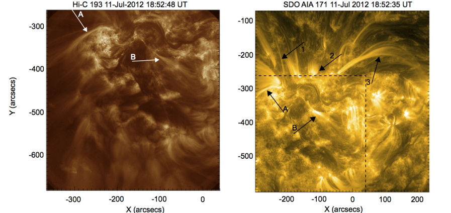
Figure 1: Active region observed with Hi-C $193$ Å (left) and SDO/AIA $171$ Å (right). The displayed AIA field of view demonstrates the extended structure of the active region and the dashed black box highlights the overlap with Hi-C. The arrows on the Hi-C image highlight the two coronal structures (labelled A and B) studied in high resolution in this paper. The same arrows are also shown on the AIA image, with the additional arrows labelled 1-3 highlighting the loop structures studied in AIA data only.

2 OBSERVATIONS AND DATA REDUCTION

The Hi-C observations took place on 11 July 2012 from 18:51:52 UT to 18:55:13 UT centred on an active region at (-130”.0,-453”.3) from disk centre. The images were obtained in the $193$ Å passband (spectral width - $5$ Å). The data was taken with a cadence of $\sim 5.4$ s and a spatial resolution of $0^{\prime\prime}.103$ per pixel ($\sim$75 km). Further details on the telescope can be found in Cirtain et al. (2013). We obtained the level 1.5, 4k$\times$4k data set through the Virtual Solar Observatory. The data was dark-subtracted, flat-fielded, cropped, dust hidden and co-aligned by the Hi-C Science team. We found that the data still displayed visible shifts from frame to frame so we additionally aligned the data using cross-correlation to achieve sub-pixel alignment. Testing the accuracy of the alignment suggests the remaining errors have a frame to frame RMS value of $0.05$ pixels. The data is missing a frame between 18:54:12-18:54:23 UT so we use linear interpolation to create the missing frame and provide a constant sampling rate for wave studies. Note that the first seven frames of the Hi-C data are inadequate for data analysis. They are displayed in figures and movies but not used for analysis.

The 193 Å line has strong contributions from Fe XII, which has a peak formation temperature close to $1.5$ MK so is ideal for observing coronal features. However, the images not only show well defined coronal loops (Fig. 1) but also spicular and fibrillar structures in and around the moss regions. The data shows that the spicules/fibrils are constantly in motion, displaying evidence for flows and waves. However, this is contrast to a corona that shows relatively muted dynamic behaviour. To analyse the motions of the fine-structure we have to perform some manipulation of the images. Due to the low signal to noise (S/N) of Hi-C, we first applied a spatial filtering algorithm to each frame to suppress the highest frequency spatial components to increase S/N. We then apply a 5 by 5 box car smoothing function to further suppress noise, while retaining sufficient signal to resolve fine-scale structure. To highlight the fine-structure an unsharp mask procedure is used (see, e.g, Fig. 2).

Due to the short duration of the Hi-C time-series, we use additional data from the SDO Atmospheric Imaging Assembly (AIA) (Lemen et al. 2011) to study the long term behaviour of the region. The data is of a larger region around the Hi-C field of view and comprises of the $171$ Å and $193$ Å bandpasses and covers the period 18:40:47-19:04:47 UT. The AIA data was prepared using the standard techniques, alignment and unsharp masking was also performed on the data sets.

3 DATA ANALYSIS

We search the data for signatures of transverse wave motion, i.e., the physical displacement of the structure’s central axis. This is performed by placing a cross-cut perpendicular to the structure under consideration and producing a time-distance diagram. To analyse the structures in the time-distance diagrams, we fit a Gaussian function to the cross-sectional flux profile in each time slice (see, e.g., Aschwanden & Schrijver 2011), which allows for sub-pixel accuracy on locating the central position of the structure’s cross-section. The fitting of the Gaussian requires an estimate of the data noise ($\sigma_{N}$), which we calculate following Yuan & Nakariakov (2012),

$$\sigma_{N}=\sqrt{\sigma_{p}(F)^{2}+\sigma_{d}^{2}+\sigma_{r}^{2}+\sigma_{sd}^{2}}=\sqrt{0.23F+588.4}.$$ (1)

where $\sigma_{p}(F)$ is the uncertainty in photon noise, $\sigma_{d}$ dark current, $\sigma_{r}$ readout and $\sigma_{sd}$ digitisation (Private communication - A. Winebarger). Similar formulae are used for the AIA data noise (Yuan & Nakariakov 2012). We also take into account errors in alignment between the frames. To determine the total error on position we add the alignment error to the Gaussian centroid position error, assuming the alignment error for each data point to be the RMS value of $0.05$ pixels for Hi-C and 0.01 for AIA data. We then supply a non-linear fitting algorithm with the central positions and the standard errors and instruct it to fit a function of the form

$$F(t)=A\sin(\frac{2\pi}{P}t-\phi)+g(t),$$

where $A,P$ and $\phi$ are the displacement amplitude, period and phase, respectively, of the wave. The parameter $g(t)$ is a linear function that represents any transverse drift of the structure with time, which could possibly be attributed to long period transverse waves. From the fitted parameters we calculate the velocity amplitude using the relation $v=2\pi A/P$.

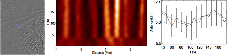
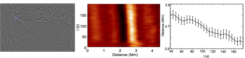
Figure 2: Top row: The left panel displays close-up, filtered images of the coronal structures labelled A and the middle panel displays a time-distance diagram for a cross-cut at the loop apex, with the cross-cut position shown in the left panel. The right panel is the results of the fitting of a loop at the apex and has measured parameters of $P=126\pm 80$ s, $A=25\pm 22$ km and $v=1.2\pm 1.3$ km/s. Bottom row: The left panel displays close-up, filtered images of the coronal structures labelled B and the middle panel displays a time-distance diagram taken close to the footpoint, with the cross-cut position shown in the left panel. The right panel is the results of the fitting to the loop. The time-scales are given in seconds from the start of Hi-C observations.

Numerous coronal structures can be observed in the Hi-C images. Two large, distinct coronal structures, arbitrarily labelled A and B, are easily identified at (-250”,-330”) and (-80”,-370”), respectively (Fig. 1 - highlighted by arrows). The rest of the coronal structures are fine loops with diffuse emission. The low S/N of the Hi-C data means any fine-structure of these diffuse loops cannot be resolved. Hence, we concentrate on the distinct coronal structures.

Example time-distance diagrams for A and B are plotted in Fig. 2. Perhaps surprisingly, these structures show little visible evidence of periodic transverse motion. For the structure A, we show a time-distance diagram taken close to the loop apex (Fig. 2 - top panels). The filtering technique has revealed this coronal structure consists of 6-7 fine threads. Fitting a Gaussian to the loop cross-sections gives loop widths of 150-310 km, suggesting the fine structure is not well resolved in the corresponding AIA $193$ Å images. This is confirmed as the unsharp masking of the AIA images does not reveal these individual loop threads (see online movies 1-4).

Upon applying the Gaussian fitting technique to the loops we are able to resolve small amplitude transverse displacement towards the foot points of the loops in structure A. A sinusiodal fit suggests the displacement is periodic (see, e.g., Fig. 3), where the measured displacement amplitude (47$\pm$14 km) is a factor of 10 smaller than the AIA pixel size. The transverse displacements can be measured along a portion of the loop leg ($\sim 2200$ km) but overlapping loops prevent us following the signal to the apex. The amplitude of the wave is seen to increase with height along the leg, from 25 km to 50 km. Cross-correlation of the signals in neighbouring slits suggests the feature is propagating with phase speeds $400\pm 300$ km s^-1. Transverse motion in a neighbouring loop in the legs also has a small displacement amplitude of $A=22\pm 12$ km, with $P=65\pm 10$ s. In contrast, measurements suggest the amplitude decreases with height. The identification of periodic transverse displacement towards the loop apex is more uncertain due to lower S/N. While the results of the fitting suggest transverse displacements with amplitudes of 10-25 km, there are large uncertainties in the fit parameters. The best example of the fits towards the loop apex is given in Fig. 2.

The changes in amplitude along the loop legs are interesting. Cross-correlation suggests the waves are propagating, implying an initial increase in amplitude could be due to decreasing density with height. We speculate that the reduction in amplitude with height could be explained by spatial damping, e.g., by invoking resonant absorption as a damping mechanism for the transverse waves (Terradas et al. 2010; Pascoe et al. 2012). Verth et al. (2010) show resonant absorption is compatible with the decrease in propagating wave amplitude along coronal loops observed in CoMP (Tomczyk & McIntosh 2009). For propagating waves, competition between amplification and damping is expected to occur in the majority of loops, with the observable variation in amplitude dependent upon the individual loop.

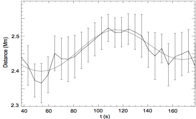
Figure 3: Results from the fitting at the footpoint of structure A (position of cross-cut given in top left panel - Fig. 2). A sinusoidal fit to the data points has measured parameters of $P=109\pm 16$ s, $A=50\pm 14$ km and $v=2.9\pm 0.9$ km/s.

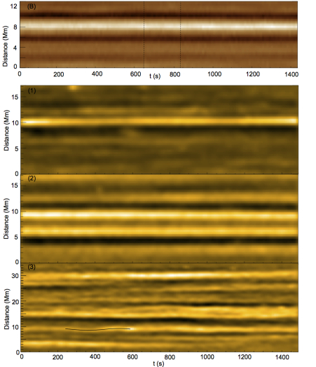
Figure 4: Time-distance diagram of the coronal feature labelled B as seen with AIA 193 Å (top panel). The time of the Hi-C observations are marked by the dashed lines. The second set of panels display time-distance diagrams for the coronal features identified as 1-3 in Fig. 1 as seen with AIA 171 Å. The time-scales are given in seconds from the start of the AIA observations.

In the second coronal structure labelled B (Fig. 2 - bottom row) there is no measurable periodic motion. The results from the fitting hint at very small amplitude periodic motion (Fig. 2: from 40-90 s), however the total displacement is below the magnitude of the uncertainties so cannot be claimed as wave motion. The linear term in the sinusoidal fit, $g(t)$, may represent a transverse motion of the loop with a long period ($>230$ s). The apparent velocity amplitude of this transverse motion is $\sim$1 km s^-1, however, we do not claim it is periodic wave motion. In Fig. 4, the time-distance diagram is shown for the AIA 193 Å data of the same spatial location. It demonstrates the activity for an extended period of time both before and after the Hi-C observations. Measurements suggest the structure does not exhibit large amplitude wave activity during the AIA observations (Fig. 4). However, we note that the coronal loop resolved in Hi-C has a width of $\sim 230$ km. This is smaller than an AIA pixel and thus AIA does not resolve the structure adequately in Fig. 4, which shows enhanced emission with a width of $\sim 600$ km, possibly indicating contributions from neighbouring features.

To gain a sense of typical wave activity in the active region, additional coronal structures in the AIA $171$ Å images are studied (labelled 1-3 in Fig. 1). The features are partially visible in the Hi-C data only for a few frames due to the shift in pointing of the telescope. Fig. 4 displays the time-distance diagrams produced for these features. The cross-cuts from structures 1 and 2 do not show any visible signs of transverse displacement. Applying the fitting routine suggests the presence of long period ($P>300$ s) and small amplitude ($A<100$ km, $v<3$ km s^-1) waves. However, the feature labelled 3 is different and displays transverse motion that is visible even to the eye (online movie 5). A cross-cut is placed near the apex of this feature (close to arrow in Fig. 1) and reveals periodic motion in numerous loop threads. One example is highlighted (over plotted black line) and the measured values are P=324$\pm$2 s, A=331$\pm$4 km, $v=6.42\pm 0.09$ km/s. However, the transverse wave motion does not appear to be continuous and only one or two wave periods are visible before the perturbation decays. Note that this decay may not be due to damping, but rather that the observed motion is a wave-packet of finite length, which travels through the cross-cut.

4 DISCUSSION AND CONCLUSIONS

With the five fold increase in resolution of Hi-C we have been able to observe transverse periodic motion ($A<50$ km) in coronal loops that would otherwise have been difficult with AIA. The Hi-C coronal loops have widths on the order of or below AIA resolution and they are not resolved by AIA. The Hi-C data only reveals small amplitude, low energy waves and some coronal structures do not show measurable periodic transverse motion even at high resolution.

The lack of identifiable wave motion in some Hi-C coronal loops could be limited by resolution still or data noise. Let us assume that the corona is filled with transverse waves and wave energy. Our results then allow us to place an upper bound on the amplitude of the transverse waves in some coronal active region structures. We suggest that transverse waves with an amplitude of $<0^{\prime\prime}.03\,(20\leavevmode\nobreak\ \mbox{km})$ (i.e., total displacement is less than half a pixel $\sim 40$ km) are at the edge of Hi-C observational limitations. Hence, any low frequency waves present with periods in the range $50-200$ s will have velocity amplitudes of $<3$ km s^-1.

A further reason for the absence of periodic transverse waves in some loops is due to the short length of the data set, $\approx$170 s (excluding the first seven frames). We assume that a wave can be detected (and fitted) if we can observe $3/4$ of a period. Hence, sinusoidal motions with periods $\gtrsim 230$ s are unable to be detected here. Signatures of long period transverse waves could be detected through the non-periodic component of the fit, $g(t)$. The transverse displacement observed in this manner also appear to have relatively small velocity amplitudes. Further, waves with periods between 200-500 s and amplitudes ¿3 km s^-1would displace the loops central axis by at least 100-400 km, something which would be measurable in both Hi-C and AIA, but is not seen.

By comparing an extended time-series taken from AIA with the short Hi-C time-series (e.g., Fig. 4), it suggests that the period of time observed by Hi-C is representative of the dynamics in the structures studied, i.e., wave activity is low for extended periods of time. Small amplitude wave activity is also observed in coronal structures identified only in AIA (1 and 2 in Fig. 1). Thus, our results suggest transverse waves supported by some active region coronal structure may have small velocity amplitudes ($<3$ km s^-1) and would not provide a significant heating contribution.

Previous observational evidence for transverse waves in active regions provided by measuring Doppler oscillations with Hinode EIS (Erdélyi & Taroyan 2008, Van Doorsselaere et al. 2010, Tian et al. 2012), reporting velocity amplitudes 1-2 km s^-1 and periods of $\sim$300 s. If these previous observations are indeed signatures of transverse waves then they are consistent with our Hi-C and AIA amplitude measurements and our upper bound. These values are also consistent with CoMP results if we assume that a significant amount of wave energy ($>90\%$) is unresolved in the CoMP data. As with previous studies, we are limited to the observation of a few active region structures for a relatively short period of time. Our results hint that there may be categories of propagating transverse waves. Namely, waves with larger velocity amplitudes ($v>$3 km s^-1) that are potentially excited by infrequent events which provide more energy flux (e.g., feature 3) than the driver of continuous (as suggested by CoMP results), small amplitude waves (¡3 km s^-1). This idea is supported by our observations, with some structures demonstrating small amplitude periodic motion (e.g., features A, B, 1, 2) and others displaying one to two periods of large amplitude motion before the displacement becomes undetectable (feature 3). However, extended studies are required to confirm this.