Renormalized vs Nonrenormalized Chiral Transition in a Magnetic Background

Abstract

We study analytically the chiral phase transition for hot quark matter in presence of a strong magnetic background, focusing on the existence of a critical point at zero baryon chemical potential and nonzero magnetic field. We build up a Ginzburg-Landau effective potential for the chiral condensate at finite temperature, computing the coefficients of the expansion within a chiral quark-meson model. Our conclusion is that the existence of the critical point at finite $\bm{B}$ is very sensitive to the way the ultraviolet divergences of the model are treated. In particular, we find that after renormalization, no chiral critical point is present in the phase diagram. On the other hand, such a critical point there exists when the ultraviolet divergences are not removed by a proper renormalization of the thermodynamic potential.

1 Introduction

Recent simulations of relativistic heavy ion collisions suggested the intriguing possibility that huge magnetic fields are created during noncentral collisions Kharzeev:2007jp ; Skokov:2009qp ; Voronyuk:2011jd . At the typical Relativistic Heavy Ion Collider energies the current estimate for the largest magnetic field produced is $eB\approx 5m_{\pi}^{2}$, with $m_{\pi}$ corresponding to the pion mass in the vacuum. Moreover, at typical Large Hadron Collider energies it is found $eB\approx 15m_{\pi}^{2}$ as a maximum value for the produced magnetic field. Electric fields are also produced in the collisions, but their magnitude is smaller than that of their magnetic counterpart. Simulations show that the structure of the electromagnetic fields in space and time is rather complicated, and in fact these fields are highly inhomogeneous and short lived. On the other hand, these results make the study of the role of the electromagnetic fields on the phase structure of Quantum Chromodynamics (QCD) not academic. Relevant studies can be found in the book Kharzeev:2012ph as well as in Bali:2011qj ; Klevansky:1989vi ; D'Elia:2011zu ; Suganuma:1990nn ; Gusynin:1995nb ; Frasca:2011zn ; Klimenko:1990rh ; Fraga:2008qn ; Agasian:2008tb ; Bruckmann:2013oba ; D'Elia:2010nq ; Endrodi:2013cs ; Fukushima:2010fe ; Mizher:2010zb ; Andersen:2012bq ; Skokov:2011ib ; Fukushima:2012xw ; Chernodub:2010qx ; Buividovich:2008wf ; Hidaka:2012mz ; Fraga:2012fs ; Preis:2010cq ; Callebaut:2013ria ; Andersen:2011ip ; Burikham:2011ng ; Filev:2010pm ; Ferrari:2012yw ; Gynther:2010ed ; Mizher:2013mia . The existence of strong fields in heavy ion collisions, combined to the excitation of strong sphalerons at high temperature Moore:1997im , also suggested the possibility of event-by-event ${\cal P}-$ and ${\cal CP}-$odd effect dubbed Chiral Magnetic Effect Kharzeev:2007jp ; Fukushima:2008xe ; Rebhan:2009vc ; Kharzeev:2010gr ; Gorsky:2010xu ; Braguta:2010ej ; Gahramanov:2012wz ; Nam:2009jb ; Wang:2012qs ; Voloshin:2010ut , see Fukushima:2012vr ; Kharzeev:2012ph for reviews. Besides heavy ion collisions, even stronger magnetic fields might have been produced in the early universe at the epoch of the electroweak phase transition, $t_{ew}$, because of gradients in the vacuum expectation value of the Higgs field: a widely accepted value for the magnetic field at the transition is $B(t_{ew})\approx 10^{5}m_{\pi}^{2}\approx 10^{19}$ T, even if this value rapidly decreased scaling as $a^{-2}$, where $a(t)$ denotes the scale factor of the expanding universe, losing several order of magnitude at the QCD phase transition. Finally, strong magnetic fields (but still weaker than the one produced in relativistic heavy ion collisions) are present on the surface of magnetars, $B\approx 10^{-4}m_{\pi}^{2}\approx 10^{10}$ T Duncan:1992hi . Therefore, there exist at least three physical contexts in which QCD in a strong magnetic background is worth to be studied.

There is general consensus on the fact that a strong magnetic field affects the physics of spontaneous chiral symmetry breaking in QCD. At zero temperature, the magnetic field induces the magnetic catalysis, leading to an increase of the chiral condensate with the strength of the applied field. On the other hand, the effect of the external field on the restoration of chiral symmetry at finite temperature is still controversial. In fact recent lattice simulations have shown that increasing the strength of the magnetic field leads to a reduction of the critical temperature for chiral restoration Bali:2011qj , which is understood in terms of the backreaction of the quark loops on the gluon action Bruckmann:2013oba . This conclusion is in agreement with some previous model computations, see for example Agasian:2008tb and Mizher:2010zb , but in disagreement with most of the recent chiral model computations. The lattice results show as well some role of the bare quark mass on the shift of the critical temperature; on the other hand, model computations have not been able to describe such a behavior, see for example Mizher:2013mia . Interesting possibilities to solve this puzzle can be found in Kojo:2012js .

Leaving apart the problem of the critical temperature, there is general agreement that the magnetic field makes the chiral phase transition stronger, and it might turn to a first order phase transition at large enough $\bm{B}$. If this is the case, then a critical point in the $(T,\bm{B})$ plane should appear at zero baryon chemical potential . Lattice results are in agreement with the strengthening of the phase transition, but they show no evidence for a critical point. The existence of the latter is also not confirmed by models: some model computations predict a first order phase transition if $eB$ is large enough, while other models do not observe a change of the phase transition from crossover to first order even for large magnetic field strengths.

In this Article we address analytically the problem of the chiral phase transition for quark matter at zero baryon chemical potential and nonzero magnetic field, focusing on the possible existence of a critical point in the phase diagram and connecting it to the ultraviolet divergences of the underlying microscopic model. In order to make quantitative predictions, we build up a Ginzburg-Landau (GL) effective potential for the chiral condensate at finite temperature; neglecting inhomogeneous condensates as well as terms which are not dependent on the condensate, we write the effective GL action around the critical line as

$$\Omega=\frac{\alpha_{2}}{2}m_{q}^{2}+\frac{\alpha_{4}}{4}m_{q}^{4}~{},$$ (1)

where $m_{q}$ corresponds to the dynamical quark mass which is proportional to the chiral condensate, see the description of the model below. According to the general GL description of a phase transition, the order of the latter depends on the sign of the coefficient $\alpha_{4}$ at the temperature $T_{c}^{*}$ defined as the solution of the equation $\alpha_{2}(T^{*}_{c})=0$. If $\alpha_{4}(T^{*}_{c})>0$ then the phase transition is of the second order and the critical temperature is $T_{c}=T^{*}_{c}$; on the other hand, if $\alpha_{4}(T_{c})<0$ then the phase transition is of the first order and the critical temperature satisfies $T_{c}>T^{*}_{c}$. Hence the point $(\alpha_{2},\alpha_{4})=(0,0)$ in the phase diagram corresponds to a critical point, at which a first order and a second order phase transition lines meet.

For the mapping of the phase diagram from the $(\alpha_{2},\alpha_{4})$ plane to the $(T,\bm{B})$ plane we need a microscopic model to compute the explicit dependence of the GL coefficients on these variables. In this Article we make use of the chiral quark-meson model Jungnickel:1995fp ; Herbst:2010rf ; Schaefer:2004en ; Skokov:2010wb , and restrict ourselves to the one-loop approximation which amounts to neglect quantum fluctuations for the meson fields in the thermodynamic potential. The advantage of the quark-meson model is its renormalizability, which allows to make quantitative predictions which are not affected by any ultraviolet scale. In fact, our main goal is to elucidate on the role of the ultraviolet divergences in this model on the order of the phase transition. Our main conclusion is that a critical point in the $(T,\bm{B})$ plane might exist, but its existence is very sensitive to the way the ultraviolet divergences of the model are treated. In particular, we are able to predict analytically that after the renormalization of the thermodynamic potential has been properly performed, no chiral critical point exists. On the other hand, such a critical point there exists when the ultraviolet divergences are not removed by a proper renormalization.

We stress that even if the model parameters are fixed having in mind the QCD spontaneous chiral symmetry breaking, our results are general and apply to any theory of charged interacting fermions in a magnetic background, when a scalar condensate appears in the theory, which we dub QCD-like theories according to a widely spread nomenclature. Keeping this in mind, it is not the scope of this Article to investigate on the discrepancy between model and Lattice computations about the effect of the magnetic field on the critical temperature of the chiral phase transition. Adding by hand a term that leads to a decreasing critical temperature in the GL second order coefficient would be an easy exercise; however we do not follow this procedure since we are not interested to a quantitative comparison with the Lattice simulations, but to a quantitative study about how ultraviolet divergences in QCD-like theories affect the physical predictions. Moreover, adding this $\bm{B}-$dependent term in the GL effective action naturally requires a further arbitrary term in the quartic coefficient, thus ruining the quantitative power of our study and the possibility to compare directly our results to those obtained within QCD-like theories.

We also stress that our purpose is not to claim that previous model computations lacking renormalization are wrong. In fact, the explicit ultraviolet cutoff appearing in the model calculations is a signal of a rough modelling of the QCD asymptotic freedom: the interactions are switched off for momenta larger than the ultraviolet scale. Therefore we consider our study as a tasteful theoretical investigation of the role of the ultraviolet divergences in the microscopic model on the order of the phase transition, rather than as a censor which judges which is the more appropriate procedure to treat the divergences of the model when it is applied to describe QCD. Nevertheless, beside the interest from the pure field theory point of view, the results can be nicely interpreted physically observing that the critical point appears naturally in the model with the explicit UV cutoff, which is a remnant of the QCD asymptotic freedom, hence connecting the latter property of the strong interactions to the existence of the former.

The plan of the Article is as follows: in Section II we describe the renormalization of the chiral quark-meson model in a magnetic background, discussing how the divergences can be embedded in the vacuum and $\bm{B}-$independent thermodynamic potential. In Section III we compute the GL coefficients of the thermodynamic potential in Eq. (1) using the renormalized model. In Section IV we repeat the same computation using the nonrenormalized model, thus leaving the explicit dependence on the ultraviolet cutoff. In Section IV we summarize our results and draw our conclusions.

2 Renormalization of the quark-meson model in a magnetic background

In this Section, we specify the model we use in our calculations, explaining its lagrangian density and how we renormalize the vacuum part of the thermodynamic potential. The lagrangian density of the model is given by

$${\cal L} = \bar{q}\left[iD_{\mu}\gamma^{\mu}-g(\sigma+i\gamma_{5}\bm{\tau}\cdot\bm{\pi})\right]q$$ (2)

$$+\frac{1}{2}\left(\partial_{\mu}\sigma\right)^{2}+\frac{1}{2}\left(\partial_{\mu}\bm{\pi}\right)^{2}-U(\sigma,\bm{\pi})~{}.$$

In the above equation, $q$ corresponds to a quark field in the fundamental representation of color group $SU(N_{c})$ and flavor group $SU(2)$; the covariant derivative, $D_{\mu}=\partial_{\mu}-Q_{f}eA_{\mu}$, describes the coupling to the background magnetic field, where $Q_{f}$ denotes the charge of the flavor $f$. Besides, $\sigma$, $\bm{\pi}$ correspond to the scalar singlet and the pseudo-scalar iso-triplet fields, respectively. The potential $U$ describes tree-level interactions among the meson fields. In this article, we take its analytic form as

$$U(\sigma,\bm{\pi})=\frac{\lambda}{4}\left(\sigma^{2}+\bm{\pi}^{2}-v^{2}\right)^{2}~{},$$ (3)

which is invariant under chiral transformations.

In this article, we restrict ourselves to the one-loop large-$N_{c}$ approximation, which amounts to consider mesons as classical fields, and integrate only over fermions in the generating functional of the theory to obtain the thermodynamic potential. As a matter of fact, quantum corrections arising from meson bubbles are suppressed of a factor $1/N_{c}$ with respect to case of the fermion bubble. In the integration process, the meson fields are fixed to their classical expectation value, $\langle\bm{\pi}\rangle=0$ and $\langle\sigma\rangle\neq 0$. The physical value of $\langle\sigma\rangle$ will be then determined by minimization of the thermodynamic potential. This implies that one replaces $g\sigma\rightarrow g\langle\sigma\rangle$ in the quark action. The field $\sigma$ carries the quantum numbers of the quark chiral condensate, $\langle\bar{q}q\rangle$; hence, in the phase with $\langle\sigma\rangle\neq 0$, chiral symmetry is spontaneously broken.

The one-loop fermion bubble associated to the interaction with a magnetic background can be computed within the Leung-Ritus-Wang method Ritus:1972ky , namely

$$\Omega_{B}=-N_{c}\sum_{f}\frac{|Q_{f}eB|}{2\pi}\sum_{n=0}^{\infty}\beta_{n}\int_{-\infty}^{+\infty}\frac{dp_{z}}{2\pi}\left[E+2T\log\left(1+e^{-\beta E}\right)\right]~{},$$ (4)

where $n$ labels the Landau level, $E$ corresponds to the single particle excitation spectrum,

$$E=\sqrt{p_{z}^{2}+2|Q_{f}eB|n+m_{q}^{2}}~{},$$ (5)

and $m_{q}=g\langle\sigma\rangle$ is the constituent quark mass. The factor $\beta_{n}=2-\delta_{n0}$ counts the degeneracy of the $n^{th}$-Landau level.

The divergence in $\Omega_{B}$ is contained in the vacuum contribution. Since the model is renormalizable, we can treat this divergence by means of renormalization. In order to prepare $\Omega_{B}$ for renormalization, we firstly add and subtract the contribution at $\bm{B}=0$, namely

$$\Omega_{0}=-2N_{c}N_{f}\int\frac{d^{3}p}{(2\pi)^{3}}\left[\omega+2T\log\left(1+e^{-\beta\omega}\right)\right]~{},$$ (6)

where $\omega=\sqrt{\bm{p}^{2}+m_{q}^{2}}$. This procedure is convenient since it allows to collect all the contributions due to the magnetic field into an addendum which is ultraviolet finite. In principle it would be enough to consider only the vacuum contribution in $\Omega_{0}$ (and in fact, such contribution will be the only one affected by the renormalization procedure); however, for the computations of the GL coefficients at finite $\bm{B}$ it is convenient to add and subtract the $\bm{B}=0$ finite temperature contribution as well. Hence we write

$$\Omega_{B}=\Omega_{0}+\left(\Omega_{B}-\Omega_{0}\right)\equiv\Omega_{0}+\delta\Omega~{}.$$ (7)

In the following we renormalize $\Omega_{0}$; then we discuss the ultraviolet behavior of $\delta\Omega$, showing that it is finite and hence it does not need to be renormalized.

2.1 Renormalization of the zero field contribution

We split the zero field potential into a vacuum and a valence part, $\Omega_{0}=\Omega_{0}^{0}+\Omega_{0}^{T}$, with

$$\Omega_{0}^{0} = -2N_{c}N_{f}\int\frac{d^{3}p}{(2\pi)^{3}}\omega~{},$$ (8)

$$\Omega_{0}^{T} = -4N_{c}N_{f}T\int\frac{d^{3}p}{(2\pi)^{3}}\log\left(1+e^{-\beta\omega}\right)~{}.$$ (9)

The valence quark contribution is finite and is not affected by renormalization. Therefore we focus on the renormalization of the vacuum part. Within a $3-$momentum UV cutoff we find, in the limit $\Lambda\gg m_{q}$ and neglecting terms which do not depend on the quark condensate,

$$\frac{\Omega_{0}^{0}}{N_{c}N_{f}}=-\frac{m_{q}^{4}}{32\pi^{2}}-\frac{m_{q}^{2}\Lambda^{2}}{4\pi^{2}}+\frac{m_{q}^{4}}{8\pi^{2}}\log\frac{2\Lambda}{m_{q}}~{}.$$ (10)

In order to remove the UV divergences we add the two counterterms to the thermodynamic potential,

$$\Omega^{c.t.}=\frac{\delta\lambda}{4}\frac{m_{q}^{4}}{g^{4}}+\frac{\delta v}{2}\frac{m_{q}^{2}}{g^{2}}~{},$$ (11)

and impose the renormalization conditions Suganuma:1990nn ; Frasca:2011zn

$$\left.\frac{\partial(\Omega_{0}^{0}+\Omega^{c.t.})}{\partial m_{q}}\right|_{m_{q}=gf_{\pi}}=\left.\frac{\partial^{2}(\Omega_{0}^{0}+\Omega^{c.t.})}{\partial m_{q}^{2}}\right|_{m_{q}=gf_{\pi}}=0~{},$$ (12)

which amount to the requirement that the one-loop contributions, represented by $\Omega_{0}$, do not affect the expectation value of the scalar field and the mass of the scalar meson. After elementary evaluation of the counterterms we find, putting $\Omega_{0}^{ren}\equiv\Omega_{0}^{0}+\Omega^{c.t.}$,

$$\frac{\Omega_{0}^{ren}}{N_{c}N_{f}}=-\frac{g^{2}f_{\pi}^{2}}{8\pi^{2}}m_{q}^{2}+\frac{3}{32\pi^{2}}m_{q}^{4}-\frac{m_{q}^{4}}{8\pi^{2}}\log\frac{m_{q}}{gf_{\pi}}~{}.$$ (13)

In this article we are interested to build up the GL expansion at the chiral critical line. To this end we need to expand the thermodynamic potential, $\Omega_{0}^{ren}+\Omega_{0}^{T}$, in powers of $m_{q}$ around $m_{q}=0$. An inspection of Eq. (13) reveals that in the zero temperature part of the thermodynamic potential a nonanalytic term, proportional to $m_{q}^{4}\log m_{q}$, is present. However this is not a problem; in fact, as discussed in Skokov:2010sf , summing up the thermal part of the potential removes the dependence on the logarithm of the quark mass, leaving an analytic function which can be expanded around $m_{q}=0$. In order to show how this cancellation occurs we take advantage of the Dolan-Jackiw large temperature expansion Dolan:1973qd , see Quiros:1999jp for a review,

$$\frac{\Omega_{0}^{T}}{N_{c}N_{f}}=-\frac{7\pi^{2}T^{4}}{180}+\frac{m_{q}^{2}T^{2}}{12}+\frac{m_{q}^{4}}{8\pi^{2}}\left[\log\frac{m_{q}}{\pi T}+\gamma_{E}-\frac{3}{4}\right]+{\cal O}\left(m_{q}^{6}/T^{6}\right)~{}.$$ (14)

Summing Eq. (13), which is valid at any temperature, to Eq. (14), which is valid only in the limit $T\gg m_{q}$ (which is the limit which we are interested to) results in the cancellation of the $\log m_{q}$ term; taking into account the meson potential Eq. (3), we find

$$\Omega_{0}^{ren}+\Omega_{0}^{T}+U=\frac{\alpha_{2}^{R}}{2}m_{q}^{2}+\frac{\alpha_{4}^{R}}{4}m_{q}^{4}+{\cal O}\left(m_{q}^{6}/T^{6}\right)~{},$$ (15)

with

$$\alpha_{2}^{R} = 2N_{c}N_{f}\left(\frac{T^{2}}{12}-\frac{g^{2}f_{\pi}^{2}}{8\pi^{2}}\right)-\frac{\lambda v^{2}}{g^{2}}~{},$$ (16)

$$\alpha_{4}^{R} = 4N_{c}N_{f}\left(\frac{\gamma_{E}-3/4}{8\pi^{2}}+\frac{3}{32\pi^{2}}-\frac{1}{8\pi^{2}}\log\frac{\pi T}{gf_{\pi}}\right)+\frac{\lambda}{g^{4}}~{},$$ (17)

and the superscript $R$ stands for renormalized. In the above equation, $\gamma_{E}$ corresponds to the Euler-Mascheroni constant.

According to the general GL theory of phase transitions, the critical temperature is obtained as a solution of the equation $\alpha_{2}^{R}=0$, that is

$$T_{c}^{2}=\frac{6\lambda v^{2}}{g^{2}N_{c}N_{f}}+\frac{3g^{2}f_{\pi}^{2}}{2\pi^{2}}~{}.$$ (18)

For numerical estimations we take the parameters of Mizher:2010zb , namely $\lambda=20$, $v=f_{\pi}$ and $g=3.3$; with this parameter set we find $T_{c}\approx 173$ MeV. Moreover $\alpha_{4}^{R}(T_{c})>0$, which implies that the phase transition is of the second order.

2.2 Ultraviolet convergence of $\delta\Omega$

Here we summarize the discussion of Frasca:2011zn which proves the ultraviolet convergence of $\delta\Omega$ in Eq. (7). Since the valence quark contribution is obviously finite, we limit ourselves to consider the $T=0$ part in $\delta\Omega$. In $\Omega_{B}$ the zero temperature contribution is

$$-N_{c}\sum_{f}\frac{|Q_{f}eB|}{2\pi}\sum_{n=0}^{\infty}\beta_{n}\int_{-\infty}^{+\infty}\frac{dp_{z}}{2\pi}E~{};$$ (19)

following Frasca:2011zn we regulate the above term introducing the function, ${\cal V}(s)$, of a complex variable, $s$, as

$${\cal V}(s)=-N_{c}\sum_{f}\frac{|Q_{f}eB|}{2\pi}\sum_{n=0}^{\infty}\beta_{n}\int_{-\infty}^{+\infty}\frac{dp_{z}}{2\pi}\left(p_{z}^{2}+2|Q_{f}eB|n+m_{q}^{2}\right)^{\frac{1-s}{2}}~{}.$$ (20)

The function ${\cal V}(s)$ can be analytically continued to $s=0$. We define then $\Omega_{B}(T=0)=\lim_{s\rightarrow 0^{+}}{\cal V}(s)$. After elementary integration over $p_{z}$, summation over $n$ and taking the limit $s\rightarrow 0^{+}$, we obtain the result

$$\Omega_{B}(T=0) = N_{c}\sum_{f}\frac{m_{q}^{4}}{16\pi^{2}}\left(\frac{2}{s}-\log(2|Q_{f}eB|)+a\right)$$ (21)

$$+N_{c}\sum_{f}\frac{|Q_{f}eB|m_{q}^{2}}{8\pi^{2}}\log\frac{m_{q}^{2}}{2|Q_{f}eB|}$$

$$-N_{c}\sum_{f}\frac{(Q_{f}eB)^{2}}{2\pi^{2}}\zeta^{\prime}\left(-1,q\right)~{}.$$

where we have subtracted terms which do not depend explicitly on the condensate. In the above equation, $\zeta\left(t,q\right)$ is the Hurwitz zeta function; we have defined $q=(m_{q}^{2}+2|Q_{f}eB|)/2|Q_{f}eB|$; furthermore, $a=1-\gamma_{E}-\psi(-1/2)$, where $\gamma_{E}$ is the Euler-Mascheroni number and $\psi$ is the digamma function. The derivative $\zeta^{\prime}\left(-1,q\right)=d\zeta(t,q)/dt$ is understood to be computed at $t=-1$.

It is shown in Frasca:2011zn that the ultraviolet divergence of the lowest Landau level (LLL) contribution is canceled by an analogous divergence coming from the higher Landau levels. Nevertheless a divergence still remains, arising from the higher Landau levels, and that is represented by the explicit $1/s$ pole in Eq. (21), which survives in the $\bm{B}\rightarrow 0$ limit and is obviously related to the divergence of the vacuum contribution which we have examined in the previous Section. The structure of the divergence in Eq. (21) is identical to that obtained within the dimensional regularization scheme; the apparent missing scale of the logarithm is hidden in the $1/s$ term, and appears explicitly when the divergence is subtracted. Such a divergence affects only the zero field, zero temperature thermodynamic potential; the corrections due to the magnetic field are either finite or independent on the condensate . As a matter of fact, taking the zero magnetic field limit we find

$$\Omega_{0}(T=0)=N_{c}N_{f}\frac{m_{q}^{4}}{16\pi^{2}}\left(\frac{2}{s}-\log m_{q}^{2}+a+\frac{1}{2}\right)~{};$$ (22)

comparing Eqs. (21) and (22) it is easily proved that the pole $2/s$ is cancelled in the difference $\Omega_{B}(T=0)-\Omega_{0}(T=0)$,

$$\delta\Omega(T=0) = -N_{c}\sum_{f}\left(\frac{m_{q}^{4}}{16\pi^{2}}+\frac{|Q_{f}eB|m_{q}^{2}}{8\pi^{2}}\right)\log\frac{2|Q_{f}eB|}{m_{q}^{2}}$$ (23)

$$-N_{c}\sum_{f}\frac{|Q_{f}eB|^{2}}{2\pi^{2}}\zeta^{\prime}\left(-1,q\right)-N_{c}N_{f}\frac{m_{q}^{4}}{32\pi^{2}}~{},$$

hence proving the statement that $\delta\Omega$ is ultraviolet finite. Since $\delta\Omega$ is finite, it does not depend on the actual regularization scheme. In fact, in the following Section we are going to use a different regularization scheme to compute the Ginzburg-Landau coefficients in the effective action for $m_{q}$ at the critical line, employing a $3-$momentum cutoff, which is certainly less elegant than the regularization scheme used in this Section, but easily manageable analytically. In that case we will prove excplicitly the cancellation of ultraviolet divergences in the relevant coefficients of the GL expansion.

Before going ahead, it is useful to remind that our goal in this article is to obtain analytically the expression of the thermodynamic potential at the critical line, within an expansion in powers of $m_{q}$. However, we notice that the argument of the log in Eq. (23) forbids the analytic expansion of the thermodynamic potential in powers of $m_{q}/|eB|$. This problem is analogous to the one encountered in the $\bm{B}=0$ case, see for example Ref. Skokov:2010sf for a nice discussion; it is well known that in the latter case, summing the valence quark contribution to the thermodynamic potential results in the replacement of the $m_{q}/\Lambda$ argument in the log in the zero temperature term with a $T/\Lambda$ argument, turning the thermodynamic potential to an analytic function of $m_{q}$ at $m_{q}=0$, then permitting the $m_{q}-$power expansion. In the case of finite $\bm{B}$ we face the same problem; as we will show explicitly in the next Section, this is cured by summing the finite temperature contribution to the thermodynamic potential.

3 Effective action at the critical line

In this Section we present the novelty of our study. Our goal is to expand $\Omega$ in powers of $m_{q}$, in order to build up the effective potential at the critical line for the order parameter. In particular, we compute the quadratic and the quartic coefficients of the Ginzburg-Landau expansion in Eq. (1), putting

$$\alpha_{i}\equiv\alpha_{i}^{R}+\delta\alpha_{i}~{}.$$ (24)

Here $\alpha_{i}^{R}$ and $\delta\alpha_{i}$ are computed from $\Omega_{0}$ and $\delta\Omega$ in Eq. (7), respectively, as $\alpha_{i}^{R}=\partial^{i}\Omega_{0}/\partial m_{q}^{i}|_{mq=0}$ and $\delta\alpha_{i}=\partial^{i}(\Omega_{B}-\Omega_{0})/\partial m_{q}^{i}|_{mq=0}$. The zero field coefficients have been computed in the previous Section, see Eqs. (16) and (17), and are the ones which are affected by the renormalization procedure. Since $\Omega_{B}-\Omega_{0}$ is finite, it is not sensitive to renormalization. In this Section we compute $\delta\alpha_{2}$ and $\delta\alpha_{4}$.

As we have stressed in the previous Section, the quantity $\Omega_{B}-\Omega_{0}$ is finite both in the ultraviolet (UV) and in the infrared (IR). However, in the intermediate steps of the computations, when the coefficients from $\Omega_{0}$ and $\Omega_{B}$ are computed independently, it is necessary to regulate the several addenda both in the UV and in the IR. We achieve this by introducing the $3-$momentum cutoffs $\Lambda$ and $\varepsilon$ respectively. However, we will prove explicitely that the final result does not depend on these cutoffs, since both the UV and the IR divergences are removed at any order in $m_{q}$ when the vacuum contribution is subtracted from the finite field one, as we have discussed in the previous Section.

In the computation of $\delta\alpha_{i}$ we find convenient use the following decomposition of $\Omega_{B}$:

$$\Omega_{B}=\Omega_{B,0}^{LLL}+\Omega_{B,T}^{LLL}+\Omega_{B,0}^{hLL}+\Omega_{B,T}^{hLL}~{},$$ (25)

where the superscripts $LLL$, $hLL$ correspond to lowest Landau level and higher Landau levels, respectively; moreover, the subscripts $0$ and $T$ correspond to the zero temperature and valence quark contributions respectively. By means of the above decomposition it is easy to identify the several contributions to each GL coefficient, as well as to check how the intermediate steps divergences combine to produce a finite result.

3.1 Computation of $\delta\alpha_{2}$

According to the definitions in Eq. (24), in order to compute $\delta\alpha_{i}$ we need to expand both $\Omega_{B}$ and $\Omega_{0}$. The computation of the zero field contribution is straightforward; we find

$$\Omega_{0}=\frac{m_{q}^{2}}{2}\left[\frac{N_{c}N_{f}}{\pi^{2}}\left(\frac{\pi^{2}T^{2}}{6}-\frac{\Lambda^{2}}{2}\right)\right]~{},~{}~{}~{}\text{at the order $m_{q}^{2}$}~{},$$ (26)

where $\Lambda$ is an intermediate-step UV cutoff which is introduced to regularize the result; as we have already stressed, when we subtract the above equation to the finite field contribution, the divergence is exactly cancelled, leaving a finite result.

Taking the second derivative of $\Omega_{B,0}^{LLL}+\Omega_{B,T}^{LLL}$ with respect to $m_{q}$ at $m_{q}=0$ we find

$$\Omega_{B,0}^{LLL}+\Omega_{B,T}^{LLL}=\frac{m_{q}^{2}}{2}\left[-N_{c}\sum_{f}\frac{|Q_{f}eB|}{2\pi^{2}}\left(\log\frac{\Lambda}{T}+a_{2}\right)\right]~{},~{}~{}~{}\text{at the order $m_{q}^{2}$}~{},$$ (27)

with $a_{2}\approx 0.139$ resulting from a convergent numerical integral. The above result is obtained by means of elementary integrations. The only care needed in the computation is to regulate the contributions coming from $\Omega_{B,0}^{LLL}$ and $\Omega_{B,T}^{LLL}$ in the IR, introducing an IR cutoff, $\varepsilon$; summing the finite temperature contribution to the zero temperature one, $\lambda$ cancels exactly leaving a finite IR result.

The computation involving the higher Landau levels is complicated by the summation over the infinite tower of levels. In order to regulate the UV divergences in the intermediate steps of the computation we use the scheme of Fukushima:2010fe , requiring that $p_{z}^{2}+2|Q_{f}eB|n\leq\Lambda^{2}$ with $\Lambda$ an UV cutoff. Then the zero temperature contribution reads

$$\Omega_{B,0}^{hLL}=\frac{m_{q}^{2}}{2}\left[-N_{c}\sum_{f}\frac{|Q_{f}eB|}{\pi^{2}}\sum_{n=1}^{N_{\Lambda}}\log\frac{\sqrt{N_{\Lambda}-n}+\sqrt{N_{\Lambda}}}{\sqrt{n}}\right]~{},~{}~{}~{}\text{at the order $m_{q}^{2}$}~{},$$ (28)

where $N_{\Lambda}=\Lambda^{2}/(2|Q_{f}eB|)$. In the above equation the summation over Landau levels has to be performed. The divergent part can be extracted analytically by using the Euler-McLaurin formula,

$$\sum_{n=1}^{N_{\Lambda}}f(n)\approx\int_{1}^{N_{\Lambda}}f(z)dz+\frac{f(1)+f(N_{\Lambda})}{2}~{},$$ (29)

while the finite part has to be computed numerically. We find, in the limit $\Lambda^{2}\gg eB$,

$$\sum_{n=1}^{N_{\Lambda}}\log\frac{\sqrt{N_{\Lambda}-n}+\sqrt{N_{\Lambda}}}{\sqrt{n}}\approx\frac{\Lambda^{2}}{2|Q_{f}eB|}+\frac{1}{4}\log\frac{2|Q_{f}eB|}{\Lambda^{2}}-b_{2}~{},$$ (30)

with $b_{2}\approx 0.806$ independent on the fermion charge, hence leading to

$$\Omega_{B,0}^{hLL}=\frac{m_{q}^{2}}{2}\left[-N_{c}\sum_{f}\frac{|Q_{f}eB|}{\pi^{2}}\left(\frac{\Lambda^{2}}{2|Q_{f}eB|}+\frac{1}{4}\log\frac{2|Q_{f}eB|}{\Lambda^{2}}-b_{2}\right)\right]~{},~{}~{}~{}\text{at the order $m_{q}^{2}$}~{}.$$ (31)

Comparing the above equation with Eqs. (26) and (27) we find that the UV divergences are perfectly cancelled, as it should.

The last computation is the thermal contribution of the higher Landau levels. This computation is a bit lengthy but straightforward. Defining

$$Y_{n}=-\frac{2T}{\pi^{2}}\sum_{f}|Q_{f}eB|\int_{0}^{\infty}dp_{z}\frac{\partial^{2}}{\partial m_{q}^{2}}\left.\log\left(1+e^{-\beta E}\right)\right|_{m_{q}=0}~{},~{}~{}~{}n\geq 1~{},$$ (32)

we have

$$\Omega_{B,T}^{hLL}=\frac{m_{q}^{2}}{2}N_{c}\sum_{n=1}^{\infty}Y_{n}~{},~{}~{}~{}\text{at the order $m_{q}^{2}$}~{};$$ (33)

in order to easily combine Eq. (33) with Eq. (26) and (27) we define $Y=\sum_{n}Y_{n}$ and

$$F_{2}=Y-\frac{T^{2}}{6}+\frac{|Q_{f}eB|}{4\pi^{2}}\log\frac{T^{2}}{2|Q_{f}eB|}~{},$$ (34)

in such a way

$$\Omega_{B,T}^{hLL}=\frac{m_{q}^{2}}{2}N_{c}\sum_{f}\left(\frac{T^{2}}{6}+\frac{|Q_{f}eB|}{4\pi^{2}}\log\frac{2|Q_{f}eB|}{T^{2}}+F_{2}\right)~{},~{}~{}~{}\text{at the order $m_{q}^{2}$}~{}.$$ (35)

We have not been able to obtain an analytic expression for $F_{2}$; on the other hand, just on the base of dimensional analysis and on the observation that $F_{2}\rightarrow 0$ in the $\bm{B}\rightarrow 0$ limit, we expect $F_{2}=(|Q_{f}eB|/\pi^{2})\times{\cal G}_{2}(|Q_{f}eB|/T^{2})$ (the overall $1/\pi^{2}$ is introduced just for convenience). In the case $|eB|/T^{2}\ll 1$ the function ${\cal G}_{2}$ can then be determined by a best fit procedure; in the opposite limit $|eB|/T^{2}\gg 1$ the thermal contribution of the higher Landau levels is suppressed, which implies $Y\rightarrow 0$ in Eq. (34). Then we find respectively ($x\equiv|eB|/T^{2}$)

$${\cal G}_{2} \approx -13.51-7.24\log x~{},~{}~{}~{}x\ll 1$$ (36)

$${\cal G}_{2} \approx -\frac{1}{4}\log 2x-\frac{\pi^{2}}{6x}~{},~{}~{}~{}x\gg 1~{}.$$ (37)

Summing up all the finite $\bm{B}$ contributions and subtracting the $\bm{B}=0$ one we thus find

$$\delta\alpha_{2}=N_{c}\sum_{f}\frac{|Q_{f}eB|}{\pi^{2}}\left[-\frac{1}{2}a_{2}+{\cal G}_{2}\left(\frac{|Q_{f}eB|}{T^{2}}\right)+b_{2}\right]~{}.$$ (38)

3.2 Computation of $\delta\alpha_{4}$

From $\Omega_{0}$ we find

$$\Omega_{0}=\frac{m_{q}^{4}}{4}\left(\frac{3N_{c}N_{f}}{2\pi^{2}}\log\frac{\Lambda^{2}}{T^{2}}-N_{c}N_{f}c_{4}^{0}\right)~{},~{}~{}~{}\text{at the order $m_{q}^{4}$}~{},$$ (39)

where $c_{4}^{0}\approx 0.265$ resulting from a finite numerical integral, and $\Lambda$ is an ultraviolet cutoff that we introduce to cut the $3-$momentum integral. At the end of the calculation, the log divergence will be cancelled by the finite $\bm{B}$ contribution, in agreement with the argument given in the previous Section.

Taking the fourth derivative of $\Omega_{B,0}^{LLL}+\Omega_{B,T}^{LLL}$ with respect to $m_{q}$ and computing it at $m_{q}=0$ we find

$$\Omega_{B,0}^{LLL}+\Omega_{B,T}^{LLL}=\frac{m_{q}^{4}}{4}\left[N_{c}\sum_{f}\frac{|Q_{f}eB|}{\pi^{2}}\frac{3}{T^{2}}a_{4}\right]~{},~{}~{}~{}\text{at the order $m_{q}^{4}$}~{},$$ (40)

In order to obtain Eq. (40) we have used an ultraviolet $3-$momentum cutoff regularization, then sent the UV cutoff to infinity being the result finite in the ultraviolet. In the above equation $a_{4}\approx 0.11$ results from a convergent numerical integral.

As for $\delta\alpha_{2}$, the computation involving the higher Landau levels is complicated by the summation over the infinite levels. In order to regulate the UV divergences in the intermediate steps of the computation we use again the regulation scheme which has lead to Eq. (28). Then the zero temperature contribution reads

$$\Omega_{B,0}^{hLL}=\frac{m_{q}^{4}}{4}N_{c}\sum_{f}\frac{3}{2\pi^{2}}\sum_{n=1}^{N_{\Lambda}}\frac{\sqrt{\Lambda^{2}-2|Q_{f}eB|n}}{n\Lambda}~{},~{}~{}~{}\text{at the order $m_{q}^{4}$}~{},$$ (41)

where $N_{\Lambda}=\Lambda^{2}/(2|Q_{f}eB|)$. In the above equation the summation over Landau levels has to be performed; the divergent contribution can be extracted once again by virtue of Eq. (29); the finite part is then computed numerically. We find, in the limit $\Lambda^{2}\gg eB$,

$$\sum_{n=1}^{N_{\Lambda}}\frac{\sqrt{\Lambda^{2}-2|Q_{f}eB|n}}{n\Lambda}\approx\log\frac{\Lambda^{2}}{2|Q_{f}eB|}-d_{4}~{},$$ (42)

with $d_{4}\approx 0.0360$, hence leading to

$$\Omega_{B,0}^{hLL}=\frac{m_{q}^{4}}{4}N_{c}\sum_{f}\frac{3}{2\pi^{2}}\left(\log\frac{\Lambda^{2}}{2|Q_{f}eB|}-d_{4}\right)~{},~{}~{}~{}\text{at the order $m_{q}^{4}$}~{}.$$ (43)

The above equation is quite useful since it allows to verify easily that once Eq. (39) is subtracted, the UV divergence is cancelled leaving a finite final result.

The last computation is the thermal contribution of the higher Landau levels. As in the case of $\delta\alpha_{2}$ the computation is a bit lenghty but straightforward. Firstly we define

$$J_{n}=-\frac{2T}{\pi^{2}}\sum_{f}|Q_{f}eB|\int_{0}^{\infty}dp_{z}\frac{\partial^{4}}{\partial m_{q}^{4}}\left.\log\left(1+e^{-\beta E}\right)\right|_{m_{q}=0}~{},~{}~{}~{}n\geq 1~{};$$ (44)

then we have

$$\Omega_{B,T}^{hLL}=\frac{m_{q}^{4}}{4}N_{c}\sum_{n=1}^{\infty}J_{n}~{},~{}~{}~{}\text{at the order $m_{q}^{4}$}~{};$$ (45)

in order to easily combine subtract Eq. (45) with Eq. (39) and (43) we define $J=\sum_{n}J_{n}$ and

$$F_{4}=J+\frac{3}{2\pi^{2}}\log\frac{T^{2}}{2|Q_{f}eB|}~{},$$ (46)

in such a way

$$\Omega_{B,T}^{hLL}=\frac{m_{q}^{4}}{4}N_{c}\left(-\frac{3}{2\pi^{2}}\sum_{f}\log\frac{T^{2}}{2|Q_{f}eB|}+\sum_{f}F_{4}\right)~{},~{}~{}~{}\text{at the order $m_{q}^{4}$}~{}.$$ (47)

As for the case of $F_{2}$, we have not been able to obtain an analytic expression for $F_{4}$ for any value of the magnetic field strength; we have limited ourselves to verify numerically that in the $\bm{B}\rightarrow 0$ limit we have $F_{4}\rightarrow-c_{4}^{0}+3d_{4}/2\pi^{2}$ independently on the fermion charge, which guarantees $\delta\alpha_{4}\rightarrow 0$ in the same limit. In the case $|eB|/T^{2}\ll 1$ a best fit procedure can be used to extract the $\bm{B}-$dependence of $F_{4}$ on the magnetic field strength; on the other hand, in the case $|eB|/T^{2}\gg 1$ the finite temperature contribution to the thermodynamic potential is dominated by the lowest Landau level, which implies $J\rightarrow 0$ in Eq. (46). We find

$$F_{4} \approx \frac{3}{2\pi^{2}}d_{4}-c_{4}^{0}~{},~{}~{}~{}x\ll 1$$ (48)

$$F_{4} \approx -\frac{3}{2\pi^{2}}\log 2x~{},~{}~{}~{}x\gg 1~{}.$$ (49)

Summing up all the finite $\bm{B}$ contributions and subtracting the $\bm{B}=0$ one we find

$$\delta\alpha_{4}=N_{c}\sum_{f}\left(\frac{3a_{4}}{\pi^{2}}\frac{|Q_{f}eB|}{T^{2}}-\frac{3}{2\pi^{2}}d_{4}+F_{4}+c_{4}^{0}\right)~{}.$$ (50)

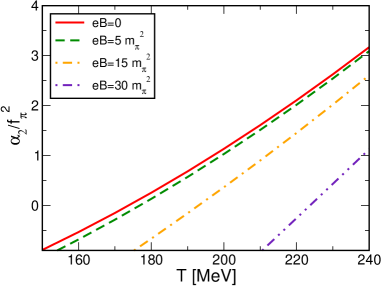
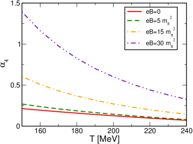
Figure 1: Coefficients $\alpha_{2}$ (left panel) and $\alpha_{4}$ (right panel) as a function of temperature, for several values of the magnetic field strength.

In Fig. 1 we plot the coefficients $\alpha_{2}$ and $\alpha_{4}$ as a function of temperature, for several values of the magnetic field strength. The location of the zeros of the quadratic coefficient is affected by the magnetic field: the larger $eB$, the larger the critical temperature. This model prediction is in disagreement with the recent lattice simulations of Bali:2011qj , but understanding the reason of the discrepancy is beyond the scope of our study. At a fixed temperature, the magnetic field increases the numerical value of $\delta\alpha_{4}$ as well, which might sound unexpected since increasing $\bm{B}$ should finally result in making the phase transition closer to a first order, hence lowering the value of $\alpha_{4}$.

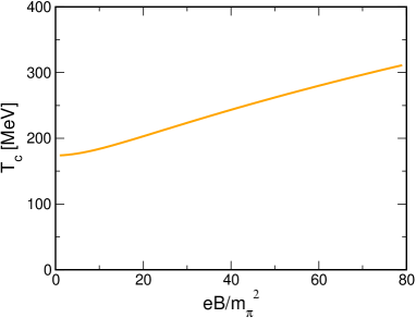
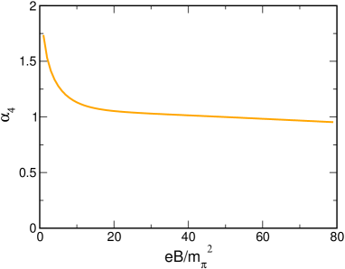
Figure 2: Critical temperature (left panel) and $\alpha_{4}$ at the critical temperature (right panel) as a function of $eB/m_{\pi}^{2}$, for the case of the renormalized model.

In order to understand why the magnetic field enhances the strength of the phase transition, we plot in Fig. 2 the critical temperature (left panel) and $\alpha_{4}$ at the critical temperature (right panel) as a function of $eB/m_{\pi}^{2}$, for the case of the renormalized model. We find that when computed at $T_{c}$, the value of $\alpha_{4}$ is a decreasing function of $eB$, thus making the phase transition closer to a first order. However, the $\alpha_{4}$ is never zero. This means that, at least within the magnetic field range we have analyzed in this study (which is however well beyond the largest magnetic fields expected to be produced in heavy ion collisions, as well as the one produced in the early universe at the QCD phase transition), no critical point is present in the phase diagram, in agreement with the lattice simulations Bali:2011qj .

3.3 Lowest Landau level approximation

It is instructive to compute the renormalized coefficients of the GL effective action in the LLL approximation, which is valid when $eB\gg T^{2}$: within the renormalized model, this amounts to consider only the LLL contribution in the thermal part of the $\bm{B}-$dependent thermodynamic potential, that is $Y=0$ in Eq. (34) and $J=0$ in Eq. (46). On the other hand, one has to be careful in defining the LLL limit in the vacuum term, because the hLLs are important to cancel the divergences arising from the expansion of $\Omega_{0}$ and of $\Omega_{0}^{LLL}$.

In the case of the second order coefficient, the hLLs vacuum term combines non trivially with the other terms, see Eq. (31); in particular, the quadratic divergence cancels with the analogous divergence in $\Omega_{0}$, while the log-type divergence combines with the same kind of divergence of the LLL to give a renormalized result $\propto|Q_{f}eB|\log 2|Q_{f}eB|/T^{2}$. Parametrically this is the leading contribution to the second order coefficient in the limit $|eB|\gg T^{2}$, and corresponds to the log-type term in the asymptotic expansion of ${\cal G}_{2}$ in Eq. (38).

For the case of the quartic order coefficient, the log-type divergence in Eq. (43) combines with the same kind of divergence in Eq. (39) to give a finite result $\propto\log 2|Q_{f}eB|/T^{2}$. However this contribution is parametrically subleading in comparison with the finite LLL contribution in Eq. (40) which is finite once we combine the $T=0$ and the finite temperature terms, and it grows up as $|Q_{f}eB|/T^{2}$. Moreover, parametrically $\alpha_{2}^{R}\ll\delta\alpha_{2}$ and $\alpha_{4}^{R}\ll\delta\alpha_{4}$ (we have verified numerically that this relation holds even for not so large values of $|eB|/T^{2}$). This observations based on the asymptotic behavior of the GL coefficients are quite interesting, since they reveal that the critical temperature is determined by a renormalized combination of the contribution of the LLL and the hLLs; hence, both the LLL and the hLLs are effective to shift $T_{c}$. However, the sign of the quartic coefficient is asymptotically determined by the LLL only, meaning that only the LLL affects the strength of the phase transition in the large field limit. Putting all together we thus find in the $|eB|/T^{2}\gg 1$ limit (the symbol $\asymp$ corresponds to asymptotic limit)

$$\alpha_{2} \asymp -N_{c}\sum_{f}\frac{|Q_{f}eB|}{4\pi^{2}}\log\frac{2|Q_{f}eB|}{T^{2}}~{},$$ (51)

$$\alpha_{4} \asymp N_{c}\sum_{f}\frac{3a_{4}}{\pi^{2}}\frac{|Q_{f}eB|}{T^{2}}~{}.$$ (52)

From Eq. (52) we read that the quartic coefficient of the GL effective action is positive in the large field limit, for every value of the temperature. This implies that the phase transition is of the second order at zero chemical potential, and this conclusion is not affected by the strength of the magnetic field.

4 Comparison with the nonrenormalized model

It is interesting to compare the results summarized in Eqs. (38) and (50) with those obtained within a nonrenormalized model. If we perform the computation of the thermodynamic potential in the latter case, the UV cutoff is kept finite and is considered a parameter, fixed to reproduce some phenomenological quantity; moreover, renormalization of the thermodynamic potential is not performed. Hence in this case the coefficients of the GL expansion at the critical line are given by the coefficients of the expansion of $\Omega_{B}$, which will contain an explicit dependence on the UV cutoff (in the case of the renormalized model, we add and subtract the zero field potential $\Omega_{0}$, which contains the UV divergences, and renormalize the latter; the difference $\Omega_{B}-\Omega_{0}$ is UV finite and does not need renormalization).

The calculation of the GL coefficients in the nonrenormalized model follow the same lines of those we have performed in the renormalized case. We introduce a $3-$momentum UV cutoff, $\Lambda$, to regulate the divergence of the zero temperature potential. The final results will depend on the numerical value of $\Lambda$.

The computation of $\alpha_{2}$ using the fixed cutoff scheme leads to the same results summarized in Eqs. (27), (28) and (33). In the present case however we cannot use the asymptotic expression in Eq. (31) since cutoff $\Lambda$ is kept fixed and the condition $\Lambda\gg|eB|$ might not apply. To the quark bubble, the contribution from the meson potential equal to $-\lambda v^{2}/g^{2}$ has to be added, see Eq. (16).

For what concerns the computation of $\alpha_{4}$, the only formal difference is in the LLL contribution, which in this case reads

$$\Omega_{B,0}^{LLL}+\Omega_{B,T}^{LLL}=\frac{m_{q}^{4}}{4}\left[N_{c}\sum_{f}\frac{|Q_{f}eB|}{\pi^{2}}\frac{3}{T^{2}}\left(a_{4}-\frac{T^{2}}{4\Lambda^{2}}\right)\right]~{},~{}~{}~{}\text{at the order $m_{q}^{4}$}~{},$$ (53)

which agrees with Eqs. (52) in the $\Lambda\rightarrow+\infty$ limit as expected. The quartic coefficient becomes negative if the critical temperature, $T_{c}$, is larger than $T_{c}^{\star}=2\Lambda\sqrt{a_{4}}\approx 0.66\Lambda$. Thus the change of the order of the phase transition seems inevitable within the nonrenormalized model, at least in the case of very large magnetic field strenghts. However this conclusion is very sensitive to the numerical value of the UV cutoff; in the limit $\Lambda\rightarrow+\infty$, the contribution in Eq. (53) is positive definite, as it happens for the case of the renormalized model, see Eq. (52). The higher Landau levels contribution is still formally given by Eqs. (41) and (45); once again, we cannot use the asymptotic form in Eq. (43) because the UV cutoff is a fixed finite number. Finally, the contribution from the meson potential equal to $\lambda/g^{4}$ has to be added, see Eq. (17).

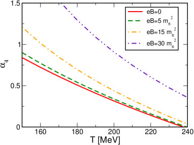
Figure 3: Coefficient $\alpha_{4}$ as a function of temperature, for several values of the magnetic field strength, in the case of the nonrenormalized model.

In Fig. 3 we plot the coefficients $\alpha_{4}$ as a function of temperature, for several values of the magnetic field strength, in the case of the nonrenormalized model. We do not plot $\alpha_{2}$ since its behavior does not change qualitatively switching from the renormalized model to the nonrenormalized one. The numerical values of the parameters are taken by Ref. Frasca:2011zn , and are $\lambda=4.67$, $\Lambda=560$ MeV and $v^{2}=-1.8m_{q}^{2}$ with $m_{q}=gf_{\pi}=335$ MeV. In this case the $v^{2}$ is negative, since the nonrenormalized quark bubble is taken into account when the requirement $\partial(\Omega_{B}+U)/\partial\sigma=0$ for $\sigma=f_{\pi}$ at $\bm{B}=0$ and $T=0$. As in the case of the renormalized model analyzed in the previous Section, increasing the value of the magnetic field strength at fixed temperature leads to an increasing of $\alpha_{4}$. This behavior seems to be counterintuitive, since the hardening of the phase transition with the magnetic field, and eventually the change of the transition from second order to first order, should occur because of a change of sign of $\alpha_{4}$; hence, one would expect that the larger the magnetic field strength, the smaller $\alpha_{4}$. However, this naive argument ignores the possibility that the critical temperature increases with the magnetic field strength, and that the GL expansion is quantitatively reliable only in the very proximity of the phase transition.

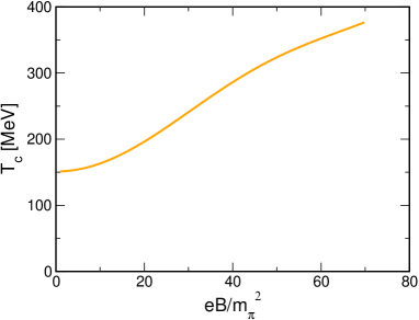
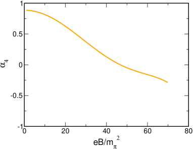
Figure 4: Critical temperature (left panel) and $\alpha_{4}$ at the critical temperature (right panel) as a function of $eB/m_{\pi}^{2}$, for the case of the nonrenormalized model. Blue dot corresponds to the critical field, $eB_{CP}\approx 47m_{\pi}^{2}$ at which the phase transition changes from a second order to a first order. The corresponding temperature is $T_{CP}\approx 313$ MeV. The calculation of the critical temperature in the left panel for $eB>eB_{CP}$ is not reliable, since higher order terms in the GL expansion should be computed in order to determine the location of the phase transition in the first order regime.

In order to explain how the phase transition changes from second order to first order in presence of a strong magnetic background, in Fig. 4 we plot the critical temperature (left panel) and $\alpha_{4}$ at the critical temperature (right panel) as a function of $eB/m_{\pi}^{2}$, for the case of the nonrenormalized model. We find that even if increasing $eB$ at fixed temperature results in making $\alpha_{4}$ more and more positive, in agreement with the behavior we find for the case of the renormalized model, the value of $\alpha_{4}$ at the critical temperature is a decreasing function of $eB$. This is due to the behavior of the critical temperature plotted in the left panel of the figure, and to the decrease of $\alpha_{4}$ with the increase of the temperature at fixed $eB$. Blue dot corresponds to the critical field, $eB_{CP}\approx 47m_{\pi}^{2}$ at which the phase transition changes from a second order to a first order. The corresponding temperature is $T_{CP}\approx 313$ MeV. The calculation of the critical temperature in the left panel for $eB>eB_{CP}$ is not reliable, since higher order terms in the GL expansion should be computed in order to determine the location of the phase transition in the first order regime.

5 Discussion and Conclusions

In this article we have computed the effective action of the chiral condensate around the chiral phase transition, in presence of a strong magnetic background $\bm{B}$. Our goal has been to understand in an analytic fashion the chiral phase transition in presence of a magnetic field, having in mind the idea of realizing if and how the second order phase transition at $\bm{B}=0$ transforms to a first order phase transition at $\bm{B}\neq 0$. We have written the effective action for the chiral condensate (or equivalently for the dynamical quark mass) around the phase transition in a Ginzburg-Landau (GL) form, see Eq. (1). For simplicity we have neglected the possibility of a coordinate dependent condensate, which allows us to neglect the gradient terms in the GL expansion. According to the general GL theory of a phase transition, the latter is of the second order if $\alpha_{4}>0$, and of first order if $\alpha_{4}<0$; the point in the phase diagram with $\alpha_{4}=0$ is called the critical point.

In order to map the phase transition lines from the $(\alpha_{2},\alpha_{4})$ plane to the $(T,\bm{B})$ plane we need a specific microscopic model. To this end we have used firstly the renormalized quark-meson model. The main scope of our study is to check the existence of a chiral critical point at $\bm{B}\neq 0$. The use of the renormalized model allows to make quantitative predictions which are not affected by an ultraviolet cutoff, which instead affects the predictions of the nonrenormalizable models. We find that no critical point appears in the phase diagram in agreement with the lattice simulations, even if the magnetic field tends to lower the value of the quartic coefficient at the critical temperature, thus making the phase transition closer to a first order one. Our result is in agreement with those of Fukushima:2010fe ; Skokov:2011ib which however are mainly numerical, while the present work is analytical, and we are able to capture the behavior of the phase transition in magnetic field in a single GL coefficient. The power of our computation is even better understood if we restrict ourselves to the LLL approximation, which is a good approximation when $eB>>T^{2}$, where we can prove analytically that the quartic coefficient is always positive, see Eq. (52). This result further excludes the existence of a critical point at large $\bm{B}$. We point out that our study is performed within the one-loop approximation; quantum fluctuations of the meson fields, which are not taken into account in our study, might modify this conclusion. However, the numerical computations of Skokov:2011ib seem to confirm that quantum fluctuations do not affect the qualitative structure of the phase diagram.

We have also compared the above results with those obtained within the nonrenormalized model, in which the ultraviolet cutoff is treated as a free parameter and its numerical value is fixed in order to reproduce few phenomenological quantities. Also in the latter case we have found the magnetic field makes the phase transition stronger. On the other hand, the sign of the quartic coefficient of the GL expansion is affected by a finite $\bm{B}$, turning the second order phase transition to a first order one. Hence, in the case of the nonrenormalized model, a critical point exists. Our main conclusion is thus that the existence of the critical point at finite $\bm{B}$ is very sensitive to the way the ultraviolet divergences of the model are treated. To make this explicit, as well as to summarize the main results we obtained, we write here below our final expressions for the quartic coefficient in the asymptotic limit $eB/T^{2}\gg 1$ for the case of renormalized model,

$$\alpha_{4}\asymp\frac{3a_{4}N_{c}}{\pi^{2}}\sum_{f}\frac{|Q_{f}eB|}{T^{2}}~{},$$ (54)

and of the nonrenormalized model,

$$\alpha_{4}\asymp\frac{3a_{4}N_{c}}{\pi^{2}}\sum_{f}\frac{|Q_{f}eB|}{T^{2}}\left(1-\frac{T^{2}}{4\Lambda^{2}a_{4}}\right)~{},$$ (55)

with $a_{4}\approx 0.11$. Clearly $\alpha_{4}$ is positive defined in the case the renormalization procedure is performed; on the other hand, its sign depends on temperature and in fact it can be negative if the critical temperature $T_{c}>2\Lambda\sqrt{a4}\approx 0.66\Lambda$. The latter result however is sensitive to the ultraviolet cutoff, and in fact the result of the nonrenormalized model tends to that of the renormalized model if one takes $\Lambda\rightarrow\infty$. However such a limit is not performed in the numerical computations based on the nonrenormalized model, since in this case $\Lambda$ is treated as a parameter whose numerical value is fixed once for all by phenomenological requirements.

We point out that the use of the nonrenormalized model, and its cutoff dependent results, is still very interesting for what concerns the applications to QCD, even if from a pure field theoretical point of view it would be preferrable to have physical predictions which are not dependent on the regularization scheme. As we explained in the Introduction, the reason is that the explicit UV cutoff appearing in the model results corresponds to a rough modelling of the QCD asymptotic freedom: the interactions are switched off for momenta larger than the UV scale. According to this interpretation of the model UV scale, our result can be rephrased in the following terms: the change of the order of the chiral transition at finite temperature and zero chemical potential, induced by the magnetic field, is mainly connected to the existence of an intrinsic UV scale, the latter being the remnant of the QCD asymptotic freedom.

There are several directions which could be followed to extend our work. One of them is the introduction of baryon chemical potential $\mu$, as well as the strange quark with its own chemical potential. In particular, since our result suggests that no critical point appears at $\mu=0$ and $\bm{B}\neq 0$, it is important to understand how the critical point at $\mu\neq 0$ and $\bm{B}\neq 0$ develops, following the analysis of Andersen:2012bq . Moreover, in our opinion it would be quite important to add a Polyakov loop background to the model, in order to realize quantitatively if and how the Polyakov loop affects the chiral phase transition. Qualitatively we do not expect a dramatic change of the results; on the other hand, a firm statement can be done only after the computation is performed. Finally, extending our study to inhomogeneous condensates following the lines of Abuki:2011pf ; Flachi:2010yz seems to be an exciting project.

- (1) D. E. Kharzeev, L. D. McLerran and H. J. Warringa, Nucl. Phys. A 803, 227 (2008).
- (2) V. Skokov, A. Y. Illarionov and V. Toneev, Int. J. Mod. Phys. A 24, 5925 (2009).
- (3) V. Voronyuk, V. D. Toneev, W. Cassing, E. L. Bratkovskaya, V. P. Konchakovski and S. A. Voloshin, Phys. Rev. C 83, 054911 (2011).
- (4) Strongly interacting matter in magnetic fields, Eds. D. Kharzeev, K. Landsteiner, A. Schmitt, H.-U. Yee, Lect. Notes Phys. (Springer); arXiv:1211.6245.
- (5) G. S. Bali et al., JHEP 1202, 044 (2012).
- (6) S. P. Klevansky and R. H. Lemmer, Phys. Rev. D 39, 3478 (1989); I. A. Shushpanov and A. V. Smilga, Phys. Lett. B 402, 351 (1997); D. N. Kabat, K. M. Lee and E. J. Weinberg, Phys. Rev. D 66, 014004 (2002); T. Inagaki, D. Kimura and T. Murata, Prog. Theor. Phys. 111, 371 (2004); T. D. Cohen, D. A. McGady and E. S. Werbos, Phys. Rev. C 76, 055201 (2007).
- (7) M. D’Elia and F. Negro, Phys. Rev. D 83, 114028 (2011); G. S. Bali et al., Phys. Rev. D 86, 071502 (2012).
- (8) H. Suganuma, T. Tatsumi and , Annals Phys. 208, 470 (1991).
- (9) V. P. Gusynin, V. A. Miransky and I. A. Shovkovy, Nucl. Phys. B 462, 249 (1996); Nucl. Phys. B 563, 361 (1999); G. W. Semenoff, I. A. Shovkovy and L. C. R. Wijewardhana, Phys. Rev. D 60, 105024 (1999); V. A. Miransky and I. A. Shovkovy, Phys. Rev. D 66, 045006 (2002).
- (10) M. Frasca, M. Ruggieri, Phys. Rev. D 83, 094024 (2011).
- (11) K. G. Klimenko, Theor. Math. Phys. 89, 1161 (1992) [Teor. Mat. Fiz. 89, 211 (1991)]; K. G. Klimenko, Z. Phys. C 54, 323 (1992); K. G. Klimenko, Theor. Math. Phys. 90, 1 (1992) [Teor. Mat. Fiz. 90, 3 (1992)].
- (12) E. S. Fraga and A. J. Mizher, Phys. Rev. D 78, 025016 (2008).
- (13) N. O. Agasian and S. M. Fedorov, Phys. Lett. B 663, 445 (2008).
- (14) F. Bruckmann, G. Endrodi and T. G. Kovacs, JHEP 1304, 112 (2013).
- (15) M. D’Elia, S. Mukherjee and F. Sanfilippo, Phys. Rev. D 82, 051501 (2010).
- (16) G. Endrodi, arXiv:1301.1307 [hep-ph].
- (17) K. Fukushima, M. Ruggieri, R. Gatto and , Phys. Rev. D 81, 114031 (2010); R. Gatto and M. Ruggieri, Phys. Rev. D 83, 034016 (2011); R. Gatto and M. Ruggieri, Phys. Rev. D 82, 054027 (2010).
- (18) A. J. Mizher, M. N. Chernodub and E. S. Fraga, Phys. Rev. D 82, 105016 (2010).
- (19) A. J. Mizher, arXiv:1304.4571 [hep-ph].
- (20) J. O. Andersen and A. Tranberg, JHEP 1208, 002 (2012).
- (21) V. Skokov, Phys. Rev. D 85, 034026 (2012).
- (22) K. Fukushima and J. M. Pawlowski, Phys. Rev. D 86, 076013 (2012).
- (23) M. N. Chernodub, Phys. Rev. D 82, 085011 (2010); Phys. Rev. Lett. 106, 142003 (2011); M. N. Chernodub, Phys. Rev. D 86, 107703 (2012); V. V. Braguta et al., Phys. Lett. B 718, 667 (2012).
- (24) P. V. Buividovich et al., Phys. Lett. B 682, 484 (2010); P. V. Buividovichet al., Nucl. Phys. B 826, 313 (2010); P. V. Buividovichet al., Phys. Rev. D 80, 054503 (2009).
- (25) Y. Hidaka and A. Yamamoto, arXiv:1209.0007 [hep-ph].
- (26) E. S. Fraga and L. F. Palhares, Phys. Rev. D 86, 016008 (2012); E. S. Fraga, J. Noronha and L. F. Palhares, arXiv:1207.7094 [hep-ph]; J. -P. Blaizot, E. S. Fraga and L. F. Palhares, arXiv:1211.6412 [hep-ph].
- (27) F. Preis, A. Rebhan and A. Schmitt, JHEP 1103, 033 (2011); F. Preis, A. Rebhan and A. Schmitt, J. Phys. G 39, 054006 (2012).
- (28) N. Callebaut and D. Dudal, arXiv:1303.5674 [hep-th]; N. Callebaut, D. Dudal and H. Verschelde, JHEP 1303, 033 (2013).
- (29) A. Gynther, K. Landsteiner, F. Pena-Benitez and A. Rebhan, JHEP 1102, 110 (2011).
- (30) J. O. Andersen and R. Khan, Phys. Rev. D 85, 065026 (2012); J. O. Andersen, Phys. Rev. D 86, 025020 (2012); J. O. Andersen, JHEP 1210, 005 (2012).
- (31) P. Burikham, JHEP 1105, 121 (2011).
- (32) V. G. Filev and R. C. Raskov, Adv. High Energy Phys. 2010, 473206 (2010); G. Lifschytz and M. Lippert, Phys. Rev. D 80, 066007 (2009).
- (33) G. N. Ferrari, A. F. Garcia and M. B. Pinto, Phys. Rev. D 86, 096005 (2012).
- (34) G. D. Moore, Phys. Lett. B 412, 359 (1997); G. D. Moore, hep-ph/0009161.
- (35) K. Fukushima, D. E. Kharzeev and H. J. Warringa, Phys. Rev. D 78, 074033 (2008); Nucl. Phys. A 836, 311 (2010); Phys. Rev. Lett. 104, 212001 (2010).
- (36) A. Rebhan, A. Schmitt and S. A. Stricker, JHEP 1001, 026 (2010).
- (37) D. E. Kharzeev and D. T. Son, Phys. Rev. Lett. 106, 062301 (2011).
- (38) A. Gorsky, P. N. Kopnin and A. V. Zayakin, Phys. Rev. D 83, 014023 (2011).
- (39) V. V. Braguta, P. V. Buividovich, T. Kalaydzhyan, S. V. Kuznetsov and M. I. Polikarpov, Phys. Atom. Nucl. 75, 488 (2012).
- (40) I. Gahramanov, T. Kalaydzhyan and I. Kirsch, Phys. Rev. D 85, 126013 (2012); A. V. Sadofyev and M. V. Isachenkov, Phys. Lett. B 697, 404 (2011).
- (41) S. -i. Nam, Phys. Rev. D 80, 114025 (2009).
- (42) G. Wang [STAR Collaboration], arXiv:1210.5498 [nucl-ex].
- (43) S. A. Voloshin, Phys. Rev. Lett. 105, 172301 (2010).
- (44) K. Fukushima, arXiv:1209.5064 [hep-ph].
- (45) R. C. Duncan and C. Thompson, Astrophys. J. 392, L9 (1992).
- (46) T. Kojo and N. Su, Phys. Lett. B 720, 192 (2013); K. Fukushima and Y. Hidaka, Phys. Rev. Lett. 110, 031601 (2013)
- (47) D. U. Jungnickel and C. Wetterich, Phys. Rev. D 53, 5142 (1996).
- (48) T. K. Herbst, J. M. Pawlowski and B. -J. Schaefer, Phys. Lett. B 696, 58 (2011).
- (49) B. -J. Schaefer and J. Wambach, Nucl. Phys. A 757, 479 (2005).
- (50) V. Skokov, B. Stokic, B. Friman and K. Redlich, Phys. Rev. C 82, 015206 (2010).
- (51) L. Dolan, R. Jackiw and , Phys. Rev. D 9, 3320 (1974).
- (52) M. Quiros, hep-ph/9901312.
- (53) V. Skokov, B. Friman, E. Nakano, K. Redlich, B. -J. Schaefer and , Phys. Rev. D 82, 034029 (2010).
- (54) V. I. Ritus, Annals Phys. 69, 555 (1972); C. N. Leung and S. Y. Wang, Nucl. Phys. B 747, 266 (2006).
- (55) H. Abuki, D. Ishibashi and K. Suzuki, Phys. Rev. D 85, 074002 (2012); H. Abuki, arXiv:1304.1904 [hep-ph].
- (56) A. Flachi and T. Tanaka, JHEP 1102, 026 (2011); A. Flachi, JHEP 1201, 023 (2012).