Strong Field Ionization as an Inhomogeneous Schrödinger Equation

Abstract

Strong field ionization is difficult to treat theoretically due to the simultaneous need to treat bound state dynamics accurately and continuum dynamics efficiently. We address this problem by decomposing the time dependent Schrödinger equation (TDSE) into an inhomogeneous form, in which a precomputed bound state acts as a source term for a time dependent tunneling component. The resulting theory is equivalent to the full TDSE when exact propagation is used, and reduces or eliminates a major source of wavefunction error when propagation is approximated. The gauge invariance of the resulting theory is used to clarify an apparent gauge dependence which has long been observed in the context of strong field S-matrix theory.

The ionization of an atom or molecule by an intense laser field is one of the basic phenomena of strong field physics, and also one of the most difficult to describe theoretically. The difficulty arises from the very different theoretical techniques needed to accurately describe the bound states of the molecule on one hand, and to efficiently describe the dynamics of the ionized electron on the other. In the zero field limit, molecular states can be well described using the methods of quantum chemistry. However, such methods typically scale poorly with system size, making them ill suited to problems in which one electron may travel dozens or hundreds of atomic units from the ionic center. Meanwhile, the dynamics of the ionized electron can be well described using single active electron calculations, at the cost of giving a poor description of the bound states. In the tunneling regime, the continuum component is typically exponentially suppressed with respect to the bound component, so that even slight errors in the treatment of the initial state have the potential to swamp the desired tunneling wavepacket.

To date, most analytical methods of strong field ionization are built around a single active electron picture, including S-matrix theoryBecker and Faisal (2005) and its variantsIvanov et al. (2005); Smirnova et al. (2007), including PPT theory Perelomov et al. (1966) and strong field eikonal-Volkov Smirnova et al. (2008); Torlina and Smirnova (2012). Methods built around quantum chemistry approaches include multiconfiguration time dependent Hartree and Hartree Fock Nest et al. (2005); Caillat et al. (2005); Zanghellini et al. (2004) and time dependent R-matrix approaches Moore et al. (2011a); Lysaght et al. (2009); Moore et al. (2011b); Tao and Scrinzi (2012). Coupled channel approaches Walters and Smirnova (2010); Torlina et al. (2012); Spanner and Patchkovskii (2009) allow interactions with the departing electron to drive transitions between different states of the ion, so that the electron “hole” may occupy any of several orbitals.

This paper addresses the problem of strong field ionization by separating the evolution of a time dependent “tunneling” component of the wavefunction from that of an initial bound state. Because the time propagator does not act upon the initial state, it may be approximated without fear of erroneously projecting the initial state into the continuum. Likewise, the initial state may be found using any desired level of theoretical approximation without increasing the computational cost of propagation. The resulting general method reproduces either the full time dependent Schrödinger equation (TDSE) or strong field S-matrix theory in the appropriate limits, and is manifestly gauge invariant. By examining its transformation under a change of gauges, we clarify a longstanding apparent gauge dependence in S-matrix theory.

I The Inhomogeneous Schrödinger Equation

When subjected to an intense laser field, an electronic wavefunction begins to deviate from its field free state. If the initial wavefunction is an eigenstate of the field free Hamiltonian $\psi_{b}(x,t)=\psi_{b}(x)e^{-iE_{b}t}$, where $H_{0}\psi_{b}=E_{b}\psi_{b}$, the full wavefunction may be written as the sum of this term plus a time dependent “tunneling” component (despite the name, the logic works equally well in the multiphoton regime)

$$\psi(t)=\psi_{b}(t)+\psi_{t}(t).$$ (1)

Mathematically, the tunneling component serves to cancel the nonzero action residual

$$\varphi(x,t)=(i\frac{\partial}{\partial t}-H(t))\phi_{b}(x,t)$$ (2)

which results when the field-free eigenstate is acted upon by the field-on Hamiltonian. Writing the full TDSE as

$$i\frac{\partial}{\partial t}(\psi_{0}e^{-iE_{0}t}+\psi_{t}(t))-(H_{0}+\delta H(t))(\psi_{0}e^{-iE_{0}t}+\psi_{t}(t))=0$$ (3)

and subtracting the evolution of the bound state due to the field free Hamiltonian

$$i\partial/\partial t\psi_{0}e^{-iE_{0}t}-H_{0}\psi_{0}e^{-iE_{0}t}=0$$ (4)

yields an inhomogeneous equation in which the laser field $H(t)-H_{0}$ acts upon the bound state to serve as a source term for the tunneling component

$$i\frac{\partial}{\partial t}\psi_{t}(t)-H(t)\psi_{t}(t)=(H(t)-H_{0})\psi_{0}e^{-iE_{0}t}.$$ (5)

Although Eqs. 3 and 5 are formally equivalent when the time propagation is exact, they will behave differently when it is approximated. In Eq. 3, the propagator acts on both the bound and the tunneling components, while in Eq. 5 it acts on the tunneling component alone.

If the Hamiltonian $H(t)$ is approximated by $\tilde{H}(t)$, where $\tilde{H}(t)=H(t)-\zeta(t)$, the Hamiltonian error $\zeta(t)$ will cause the propagated wavefunction to deviate from the true wavefunction. Writing the true tunneling component $\psi_{t}(x,t)=\phi_{t}(x,t)+\epsilon(x,t)$ as the sum of the propagated component plus an error term, then propagating $\phi_{t}$ using the approximate Hamiltonian, so that

$$(i\frac{\partial}{\partial t}-\tilde{H})(\psi_{b}(x,t)+\phi_{t}(x,t))=0,$$ (6)

causes the error term to obey an inhomogeneous Schrödinger equation

$$i\frac{\partial}{\partial t}\epsilon(t)-H(t)\epsilon(t)=\zeta(t)(\psi_{b}(x,t)+\phi_{t}(t)),$$ (7)

where the Hamiltonian error $\zeta(t)$ acts upon both the bound and the tunneling components of the propagated wavefunction to serve as a source term for the error. If the tunneling component is small relative to the bound state component, the dominant source of error is the Hamiltonian error acting upon the bound state. Thus, a small error requires that $\psi_{b}$, an eigenstate of the true Hamiltonian $H(t)$, be accurately described by the approximate Hamiltonian $\tilde{H}(t)$ used in the propagation.

In contrast, Eq. 5 allows for two approximations to the Hamiltonian – the approximation $\tilde{H}_{B}=H_{0}-\zeta_{B}$ used to find $\phi_{B}$, and the approximation $\tilde{H}_{t}(t)=H(t)-\zeta_{t}(t)$ used to propagate $\phi_{t}$. In terms of these Hamiltonians, the wavefunction error now obeys

$$i\frac{\partial}{\partial t}\epsilon_{t}(t)-H(t)\epsilon_{t}(t)=\zeta_{B}\psi_{B}(x,t)+\zeta_{T}(t)\psi_{t},$$ (8)

so that the error in the bound state Hamiltonian operates on the bound state, and the error in the propagation Hamiltonian acts on the tunneling component. The advantage of the inhomogeneous TDSE, then, is the freedom to choose a different (presumably better) approximation to the Hamiltonian when finding the initial bound state than will subsequently be used in the propagation. Doing so will reduce or eliminate the major source of error in Eq. 7 at the cost of finding a single, static eigenfunction of $\tilde{H}_{B}$, while leaving the cost of propagation essentially unchanged.

I.1 Gauge Transformation

The use of an inhomogeneous Schrödinger equation has a long history in analytical approaches to strong field ionization, in particular strong field S-matrix theory Ivanov et al. (2005); Smirnova et al. (2007). Here, the molecular potential is often ignored completely after the moment of ionization, so that the tunneling component can be expanded in a basis of Volkov states $\phi_{t}=\int dpC_{p}\ket{p-eA(t)}$, where $p$ is the conjugate momentum of the electron in the laser field, $e=-1$ is the charge of the electron, and

$$C_{p}=-i\int_{0}^{t}dt^{\prime}e^{-i\frac{1}{2}(p-eA(t^{\prime\prime}))^{2}dt^{\prime\prime}}\bra{p-eA(t)}V_{L}(t^{\prime})\ket{\phi_{b}}e^{-iE_{b}t^{\prime}}$$ (9)

or, in differential form,

$$(i\frac{\partial}{\partial t}-\frac{1}{2}(p-eA(t))^{2})C_{p}=e^{-ieA(t^{\prime})x}\bra{p}V_{L}(t^{\prime})\ket{\phi_{b}}e^{-iE_{b}t^{\prime}}.$$ (10)

An apparent gauge dependence now arises from the question of what gauge $V_{L}(t)=H(t)-H_{0}$ is to be calculated in. As the Volkov states are stationary in the velocity gauge, it may seem natural to calculate $V_{L}$ in this gauge as well. However, comparisons with the numerical TDSE have shown Becker and Milošević (2009) better agreement when $V_{L}$ is calculated in the length gauge. Although perfect gauge invariance cannot be expected when ignoring the molecular potential, such discrepancies have been seen as well in the ionization of negatively charged ions, where the strong field approximation is better justified. As gauge invariance is an essential feature of a physical theory, a brief digression is warranted.

As written, Eqs. 3 and 5 are manifestly gauge invariant. Rewriting the right hand side of Eq. 5 as

$$(H-H_{0})\psi_{0}e^{-iE_{0}t}\rightarrow(i\frac{\partial}{\partial t}-H(t))\psi_{0}e^{-iE_{0}t},$$ (11)

Eq. 5 becomes

$$i\frac{\partial}{\partial t}\psi_{t}(t)-H(t)\psi_{t}(t)=\varphi(x,t)=(i\frac{\partial}{\partial t}-H(t))\psi_{0}e^{-iE_{0}t},$$ (12)

so that Eq. 3 and both sides of Eq. 12 have the form

$$\varphi(x,t)=(i\frac{\partial}{\partial t}-H(t))\psi(x,t),$$ (13)

where $\varphi(x,t)$ can be thought of as an action residual which arises when $\psi(x,t)$ does not satisfy the Schrödinger equation perfectly. If we now perform the gauge transformation $\psi(x,t)\rightarrow\psi(x,t)e^{i\Lambda(x,t)}$, $\vec{A}(x,t)\rightarrow\vec{A}(x,t)-\vec{\nabla}\Lambda(x,t)$, $\phi(x,t)\rightarrow\phi(x,t)+\frac{\partial}{\partial t}\Lambda(x,t)$, then transforming the action residual according to $\varphi(x,t)\rightarrow\varphi(x,t)e^{i\Lambda(x,t)}$ preserves equality. In Eq. 3, $\varphi(x,t)=0$ is unaffected by the change of gauge, while in Eq. 12, $\varphi(x,t)$ is affected in the same way by transforming both sides of the equation, so that the theory as a whole is gauge invariant.

The apparent gauge dependence which is seen in strong field S-matrix theory arises from calculating the source term in one gauge and the tunneling component in another. Thus, it is equivalent to transforming one side of Eq. 5 but not the other. It is therefore not a true gauge transformation which causes the observed results, but rather a subtle modification of the effective source term. If we reverse the one sided transformation, so that both sides are calculated in the same gauge, the effective source term will not be the field free bound state $\psi_{b}(t)$, but rather $\psi_{b}(t)e^{-i\Lambda(x,t)}$. For the specific case of strong field S-matrix theory, the action residual from Eq. 10 becomes

$$\begin{split}\varphi(x,t)=&e^{-ie\vec{A}(t)\cdot\vec{x}}\vec{E}(t)\cdot\vec{x}\psi_{b}(x)e^{-iE_{b}t^{\prime}}\\ \rightarrow&(\frac{(\vec{p}-e\vec{A}(t))^{2}}{2}-\frac{|\vec{p}|^{2}}{2})\psi_{b}(x)e^{-iE_{b}t^{\prime}}e^{-ie\vec{A}(t)\cdot\vec{x}},\end{split}$$ (14)

so that the effective source term when calculated in the same gauge as the tunneling component becomes $\psi_{b}(t)e^{-iE_{b}t^{\prime}}e^{-ie\vec{A}(t)\cdot\vec{x}}$. The improved accuracy of the “length gauge” calculation can now be explained by noting that the effective source wavefunction

$$\psi_{b}(x,t)=\psi_{0}e^{-E_{b}t}e^{-ie\vec{A}(t)\cdot\vec{x}}$$ (15)

obeys

$$i\frac{\partial}{\partial t}\psi_{b}(x,t)=(H_{0}+\vec{E}(t)\cdot\vec{x})\psi_{b}(x,t),$$ (16)

so that it is a quasistatic eigenfunction of the field-on Hamiltonian rather than a static eigenfunction of the field-off Hamiltonian. By incorporating the dressing of the bound state by the laser field into the source term rather than the tunneling component, a correspondingly smaller fraction of the dynamics must be treated using the inexact propagation Hamiltonian, giving a simple explanation for the improved accuracy.

II Numerical Propagation

II.1 Least Action Propagator

The inhomogeneous form of the Schrödinger Equation may be propagated using methods similar to those used for the homogeneous form. For this paper, we propagated both forms using the least action propagator Walters (2011). For each timestep, we expanded both the bound and the tunneling components of the wavefunction with respect to a spacial basis $\chi_{i}(x)$ and a temporal basis $T_{n}(t)$, so that $\phi(x,t)=\phi_{0}(x,t)+\phi_{t}(x,t)=\sum_{i,n}D_{i,n}\chi_{i}(x)T_{n}(t)$. The expansion coefficients $D_{in}$ were found by minimizing the action accumulated by the wavefunction over the chosen timestep. By choosing finite bases in space and time, this can be accomplished by solving a linear system of equations for $D_{in}$. In order to reduce computational cost, our spatial basis was chosen to yield banded matrices, while our temporal basis was constructed to allow for eigenvector decomposition.

For a time dependent Hamiltonian $\tilde{H}(t)$ and temporal interval $[t_{0},t_{0}+\Delta t]$, the action accumulated over the timestep is minimized when

$$(iO_{ij}Q_{nm}-\tilde{H}_{ijnm})D_{jm}=0$$ (17)

for all $i,n$ such that $D_{in}$ is a free parameter (some values of $D_{in}$ will be fixed by the choice of initial or boundary conditions). Here $O_{ij}=\braket{\chi_{i}}{\chi_{j}}$ is the spatial overlap matrix, $Q_{ij}=\bra{T_{n}}\frac{\partial}{\partial t}\ket{T_{m}}$ is the temporal derivative matrix, and $\tilde{H}_{ijnm}=\bra{\chi_{i}T_{n}}\tilde{H}(t)\ket{\chi_{j}T_{m}}$ is the (time dependent) Hamiltonian matrix. For a static Hamiltonian, $\tilde{H}_{ijnm}=\tilde{H}_{ij}U_{nm}$, where $U_{nm}=\braket{T_{n}}{T_{m}}$ is the temporal overlap matrix and $\tilde{H}_{ij}=\bra{\chi_{i}}\tilde{H}\ket{\chi_{j}}$ is the Hamiltonian matrix.

Separating the bound and tunneling components as in Eq 5 yields a linear system with a nonzero right hand side. In action language, the laser field causes the bound state to accumulate nonzero action, which must be canceled by the evolution of the tunneling component. Writing the tunneling component as $\phi_{t}(x,t)=\sum_{i,n}C_{in}\chi_{i}(x)T_{n}(t)$ and the field free bound state component as $\phi_{0}=\sum_{i,n}B_{in}\chi_{i}(x)T_{n}(t)$, the least action equation becomes

$$(iO_{ij}Q_{nm}-\tilde{H}_{ijnm})C_{jm}=\Delta\tilde{H}_{ijnm}B_{jm},$$ (18)

where $\Delta\tilde{H}_{ijnm}=\bra{\chi_{i}T_{n}}\Delta\tilde{H}_{B}(t)\ket{\chi_{j}T_{m}}$.

In the velocity gauge, the kinetic energy term of the Hamiltonian is given by $\tilde{H}(t)=\frac{1}{2}(\vec{p}-e\vec{A}(t))^{2}$, where $A(t)$ is the time dependent vector potential, with matrix elements $A_{nm}=\bra{T_{n}}A(t)\ket{T_{m}}$ and $A^{2}_{nm}=\bra{T_{n}}A^{2}(t)\ket{T_{m}}$ for its square. The squared term is often neglected in numerical treatments, but is required here for gauge invariance and for use with exterior complex scaling. The least action linear system is now

$$\begin{split}[iO_{ij}Q_{nm}-(-\triangle_{ij}U_{nm}-\frac{i}{2}\nabla_{ij}A_{nm}&\\ +\frac{i}{2}\nabla^{{\dagger}}_{ij}A_{nm}+\frac{1}{2}O_{ij}A^{2}_{nm}+V_{ij}U_{nm}&)]C_{jm}=R_{in},\end{split}$$ (19)

where $R_{in}$ is the inhomogeneous source term, $\nabla_{ij}=\bra{\chi_{i}}\nabla\ket{\chi_{j}}$ is the matrix element of the gradient and $\triangle_{ij}=\bra{\chi_{i}}\triangle\ket{\chi_{j}}$ is the matrix element of the Laplacian. As discussed earlier, the gauge in which $R_{in}$ is found may be varied, with a corresponding change in the effective bound state. For this paper, we calculated $R_{in}$ in both the velocity gauge

$$R_{in}=(-\frac{1}{2}i\nabla_{ij}A_{nm}+\frac{1}{2}i\nabla^{{\dagger}}_{ij}A_{nm}+\frac{1}{2}O_{ij}A^{2}_{nm})B_{jm}$$ (20)

and the length gauge

$$O_{ij}U_{nm}R_{jm}=\braket{\chi_{i}(x)T_{n}(t)}{e^{-iA(t)x}x\phi_{b}(x,t)}.$$ (21)

The linear system constructed in this way requires a large number of coefficients to be found at every timestep – for a spatial basis set of size $N_{x}$ and a temporal basis set of size $N_{t}$, $N_{x}\cdot N_{t}$ coefficients must be found at every timestep. We chose our spatial and temporal basis sets so as to decompose this problem into the iterated solution of $(N_{t}-1)$ sparse, banded linear systems for $N_{x}$ coefficients apiece, so that every timestep required computational effort on the order of $N_{x}N_{t}$.

II.2 Spatial basis

Our spatial basis was constructed following Scrinzi (2010) to allow for infinite range exterior complex scaling. For a one dimensional problem, the region $-\infty<x<\infty$ is divided into a number of finite elements, plus two semi-infinite end caps. Within each element, the wavefunction is described using a primitive basis of low order Legendre polynomials. In each end cap, the primitive basis set is given by Laguerre polynomials times declining exponentials, so that the wavefunction is required to be 0 at $x=\pm\infty$. In contrast to Scrinzi (2010), here the same order polynomials were used in each element and both end caps.

We dealt with the problem of reflections from the borders of the propagation region by employing infinite range exterior complex scaling. Beyond some scaling radius $x_{ecs}$, we analytically rotated $x\rightarrow x_{ecs}+(x-x_{ecs})e^{-i\theta}$, so that a wavefunction of the form $e^{ikx}$ will go to zero as $x$ goes to infinity. This was accomplished by multiplying $O_{ij}\rightarrow O_{ij}e^{-i\theta}$, $\triangle_{ij}\rightarrow\triangle_{ij}e^{i\theta}$, $V_{ij}\rightarrow V_{ij}e^{-i\theta}$ for all elements beyond $x_{ecs}$. Because exterior complex scaling causes a derivative discontinuity at $x_{ecs}$, it is necessary to enforce an element boundary at $x_{ecs}$. In contrast to Scrinzi (2010), we include a number of finite elements in the scaled region in addition to the semi-infinite end caps. The inner boundary $x_{b}$ of the end caps was chosen such that $e^{-k|x_{b}-x_{ecs}|}$, where $k=\sqrt{2E_{max}}$, was less than some tolerance.

Aside from enforced element boundaries at $x=0$ and $x=\pm x_{ecs}$, the size of an individual element was determined using a WKB approach. Choosing an energy cutoff $E_{max}$ and a maximum phase $\Delta\phi$ to be accumulated in an element, the size $\Delta x$ of an element was given by $\Delta\phi=\Delta x\sqrt{2(E_{max}+|V(x)|+|Fx|)}$, where $F$ is the maximum strength of the laser field. Constructing the spatial basis in this way ensures that a local Hamiltonian will yield sparse, banded spatial matrices, with a bandwidth determined by the order of the polynomials in the primitive basis set. Highly oscillatory functions can be treated by decreasing the size of the finite elements, or by increasing the order of the polynomials used inside each element.

Wavefunction continuity across element boundaries was enforced by constructing linear combinations of the primitive basis sets. Within each element, we constructed left border functions $BF_{L}(y)=\frac{1}{2}(P_{0}(y)-P_{1}(y))$, right border functions $BF_{R}(y)=\frac{1}{2}(P_{0}(y)+P_{1}(y))$, and interior functions $BF_{n}(y)=(P_{n}(y)-P_{n\mod 2}(y))$ for $n\geq 2$, where $y$ is a local coordinate equal to $-1$ at the left boundary and $1$ at the right boundary. Recalling that $P_{l}(-1)=(-1)^{l}$ and $P_{l}(1)=1$, it can be seen that $BF_{L}$ is the only nonzero function at the left boundary and $BF_{R}$ is the only nonzero function on the right boundary. Wavefunction continuity was enforced by requiring the temporal coefficients $C_{in}$ of the left border function in one element to equal the coefficients of the right border function in the element to the left, and vice versa. Border functions in the end caps were defined in an analogous way using Laguerre rather than Legendre polynomials.

II.3 Temporal basis

While the spatial basis was constructed to yield sparse, banded spatial matrices and to enforce wavefunction continuity, the temporal basis set was constructed to reduce the size of the linear systems which must be solved at every timestep. Linear combinations of the primitive Legendre basis were constructed so that only one basis function was nonzero at the beginning of the timestep, while the other basis functions had a tridiagonal overlap structure. Using local coordinate $\tau$, equal to $-1$ at the beginning of the timestep and $+1$ at the end, we set $T_{0}(t)=\frac{1}{2}(P_{0}(\tau)-P_{1}(\tau))$ and $T_{n}(t)=\frac{1}{2}(P_{n}(\tau)+P_{n-1}(\tau))$, where $P_{n}(\tau)$ is the Legendre polynomial of order n. Note that $T_{0}(t_{0})=1$, $T_{0}(t_{0}+\Delta t)=0$, and $T_{n}(t_{0})=0$, $T_{n}(t_{0}+\Delta t)=1$ for $n\geq 1$. Thus, the wavefunction at the beginning of the step is given by the coefficients of the zeroth order basis function, while the wavefunction at the end of the pulse is given by the sum of the coefficients of all the nonzero basis functions.

The size of the linear systems to be solved can be reduced by performing an eigenvector decomposition of the residuals $R_{in}$, $n\geq 1$, which must be eliminated by the tunneling wavefunction. (Because $C_{i0}$ are not free parameters, $R_{i0}$ will not in general be canceled by the minimum action solution.) Noting that for small timesteps $A(t)$ and $A^{2}(t)$ are approximately constant, so that $A_{nm}\approx aU_{nm}$ and $A^{2}_{nm}\approx bU_{nm}$, the residuals can be projected onto generalized eigenvectors of the $Q$ and $U$ matrices. Setting $\tilde{Q}_{nm}=Q_{nm}$ and $\tilde{U}_{nm}=U_{nm}$ for $n,m\geq 1$, $\tilde{U}$ and $\tilde{Q}$ have right and left eigenvectors

$$\tilde{Q}v^{\alpha}=\lambda^{\alpha}\tilde{U}v^{\alpha}$$ (22)

and

$$w^{\alpha}\tilde{Q}=\lambda^{\alpha}w^{\alpha}\tilde{U},$$ (23)

where $\lambda^{\alpha}$ is a generalized eigenvalue and $w^{\alpha{\dagger}}\tilde{U}v^{\beta}=\delta_{\alpha\beta}$. Ignoring $(A_{nm}-aU_{nm})$ and $(A^{2}_{nm}-bU_{nm})$ for the moment, if $\delta C_{jm}=\sum_{\alpha}C^{\alpha}_{j}v^{\alpha}_{m}$, then

$$(iO_{ij}\lambda^{\alpha}-(-\nabla^{2}_{ij}-ia\nabla_{ij}+ia\nabla^{{\dagger}}_{ij}+bO_{ij}+V_{ij}))\delta C^{\alpha}_{j}=\sum_{n}w^{\alpha{\dagger}}_{n}R_{in}.$$ (24)

Because this method neglects the differences $(A_{nm}-aU_{nm})$ and $(A^{2}_{nm}-bU_{nm})$, it will yield an approximate rather than exact solution for $\delta C^{\alpha}_{j}$, so that applying the correction $C_{in}\rightarrow C_{in}+\delta C_{in}$ will not cancel the residuals completely. However, as a single timestep will typically be very short compared to the frequency of the driving laser, the variation of $A(t)$ and $A^{2}(t)$ over a single timestep will be very small, and repeated application of this procedure will yield rapid convergence to zero residual. We repeat this iteration until $\delta\psi_{t}(x,t+\Delta t)=\sum_{n}\delta C_{in}$ has a norm less than some desired tolerance. After finding the minimum norm solution, we adjust the size of the next step so that the contribution of the last temporal basis function to the final wavefunction $\delta\psi_{n_{max}}=\sum_{i}C_{in_{max}}\chi_{i}(x)$ has a norm less than a chosen accuracy goal.

Having found the variationally optimum description of the wavefunction in the chosen basis, the timestep may now be adjusted to ensure that the wavefunction evolution is well described by the temporal basis. We ensure this by choosing a timestep such that the last Legendre polynomial included in the primitive basis has a negligible contribution to the total solution. If

$$F_{i}=U^{-1}\sum_{n}C_{in}\braket{P_{n_{max}}}{T_{n}}$$ (25)

is the vector of spatial coefficients for the last Legendre polynomial and

$$\delta\psi_{n_{max}}=\sum_{i,j}F^{*}_{i}O_{ij}F_{j},$$ (26)

is its norm, then

$$\frac{\Delta t^{\prime}}{\Delta t}=(\frac{\text{accuracy goal}}{\delta\psi_{n_{max}}})^{n_{max}-1}$$ (27)

gives the ratio of the new time step to the old.

These design choices yield a variable stepsize, variationally optimum propagator for a wavefunction described in a finite element basis. The order of the polynomials used to describe the wavefunction within each element, as well as the temporal order used to describe the wavefunction over a given timestep, can be chosen at will. The linear systems which must be solved are sparse, banded, and do not grow with increasing temporal order. For the calculations in this paper, we used polynomials of order 5 for both our spatial and temporal bases, and propagated with an accuracy goal of $10^{-6}$. As the spatial component $\delta\psi_{n_{\text{max}}}$ of the last temporal basis function vanishes very rapidly with increasing $n_{\text{max}}$, the maximum step size was limited, not by the accuracy of the propagator, but rather by the accuracy of a polynomial expansion for the temporal evolution $e^{iE_{g}t}$ of the source wavefunction.

III Results

We illustrate our treatment of strong field ionization by comparing the evolution of the tunneling component to that of the full wavefunction resulting from half a cycle of an intense laser pulse. For our model atom we use a one dimensional soft core potential $V(x)=-\frac{Q}{\sqrt{a^{2}+x^{2}}}$, where $Q=a=1$, whose ground state has energy $E_{g}=-0.670$. For laser electric field $E(t)=F_{0}\cos(\omega t)$, we set $F_{0}=0.05$ and $\omega=0.0565$ (equivalent to an intensity of $8.9\times 10^{13}$ W/cm², consistent with many strong field experiments). The combination of ground state and laser pulse yielded a Keldysh parameter $\gamma=1.31$, placing it in the intermediate range between the tunneling and multiphoton limits.

We compare the evolution of the full wavefunction to that of the tunneling component using three different potentials for the propagator. First, we verify that our approach gives results identical to the homogeneous TDSE by comparing comparing their evolution using the exact propagator. We then demonstrate the effects of an imperfect propagator by intentionally distorting the potential used in propagation. We perform one calculation using $V(x)=0$ (the well known strong field approximation) and one with $V(x)=-\frac{Q}{\sqrt{a^{2}+x^{2}}}$ with $a\rightarrow 2.0$, so that the potential is asymptotically correct but differs from the correct potential at short range. Such a distortion is analogous to those which might arise in a single active electron mean field calculation, where the electron’s interaction with the ion is correct at long range but differs from the true potential at short range.

In Figures 1 and 2, we show that the inhomogeneous Schrödinger equation is identical to the homogeneous form for both the velocity and length gauge source terms. As discussed earlier, use of the “length gauge” source term is equivalent to using a quasistatic rather than a static wavefunction in the velocity gauge source term. In the present context, this means that the initial condition for the full wavefunction, when $\psi_{t}(x,t_{i})=0$, must be the static bound state $\psi(x,t_{i})=\psi_{g}e^{-iE_{g}t_{i}}$ for comparison with the velocity gauge calculation, and the quasistatic state $\psi(x,t_{i})=\psi_{g}e^{-iE_{g}t_{i}}e^{-i\vec{A}(x,t)\cdot\vec{x}}$ for comparison with the length gauge. As seen in these figures, both source terms give results which are identical to the full wavefunction in the region where $\psi_{g}(x)=0$. The apparent gauge dependence is thus reconciled: both gauges give results which are equivalent to the full TDSE, and differ from each other only due to the use of different source terms.

The strong field approximation is shown in Figures 3 and 4. Here setting $V(x)=0$ means that the propagator is incapable of treating a bound state correctly, so that the entire propagated wavefunction is projected into the continuum. As might be expected, propagating the full wavefunction gives results which bear no resemblance to the true behavior. In contrast, the inhomogeneous approach allows the propagator only to act on that portion of the wavefunction which differs from the initial bound state. Here the tunneling components have magnitudes similar to the true tunneling components, with peaks somewhat displaced due to the different potentials seen by the continuum wavefunctions. As the strong field approximation is commonly used in analytical treatments of strong field ionization, we show in Figure 4b the PPT tunneling component taken from Ivanov et al. (2005). As in Ivanov et al. (2005), only the exponential suppression due to tunneling is calculated, so that the ionization amplitude has only exponential accuracy. The PPT wavepacket is much more localized than either the true tunneling component or the propagated strong field result, and has a considerably smaller amplitude. As interactions with the departing electron may cause dynamics within the parent ion, this may be an indication that more sophisticated treatments of strong field ionization will be necessary to describe processes such as multichannel ionization.

For our third calculation, we observe the results of a distorted short range potential in Figures 5 and 6. In contrast to the strong field approximation, this propagator treats the wavefunction correctly when it is far from the molecule, but incorrectly when the electron is nearby. Thus, propagating the full wavefunction will cause bound states to be projected into the continuum, but the continuum wavepacket will evolve correctly for most of its journey.

In the velocity gauge calculation, the full wavefunction shown in Figure 5a has a very similar peak structure to the exact solution, but overestimates the amplitude of the wavefunction far from the origin. The tunneling component in Figure 5b has amplitude comparable to the exact solution, but the maxima of the tunneling component are displaced somewhat from the exact solution.

For the length gauge calculation, the incorrect potential causes the initially quasistatic wavefunction to diverge strongly from the exact solution in Figure 6a, as a portion of the initial state is projected into the continuum. In contrast, Figure 6b shows a strong similarity between the exact and approximated tunneling components, with maxima which are once again displaced from the exact solution.

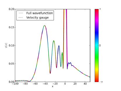
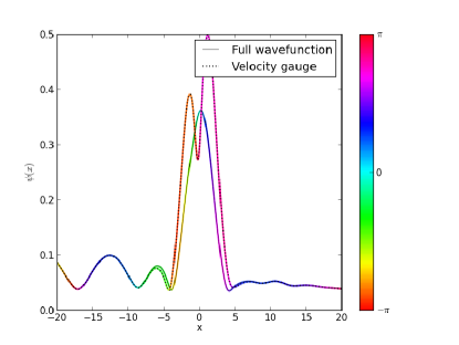
Figure 1: a) Tunneling component vs full wavefunction using velocity gauge source term b) Same calculation near the origin. The tunneling component equals the full wavefunction in the region where the source wavefunction is zero, and differs where it is not. Lines show wavefunction magnitude, while color indicates phase.

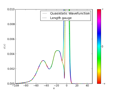
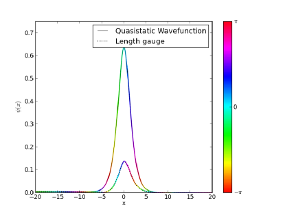
Figure 2: a) Tunneling component vs full wavefunction using length gauge source term b) Same calculation near the origin. The tunneling component equals the full wavefunction in the region where the source wavefunction is zero, and differs where it is not. The initial condition for the full wavefunction is the quasistatic eigenfunction rather than the field free eigenstate. Lines show wavefunction magnitude, while color indicates phase.

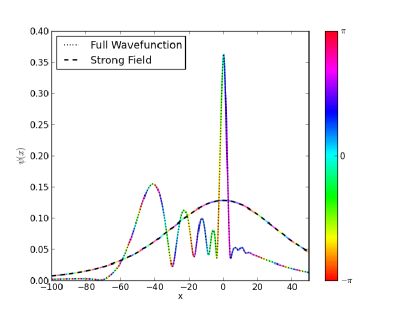
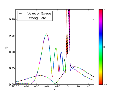
Figure 3: a) Full wavefunction propagated using exact propagator vs strong field propagator b) Velocity gauge tunneling component propagated using exact propagator vs strong field propagator. Whereas propagation of the full wavefunction fails completely for the strong field propagator, the tunneling component has comparable magnitude to that found using the exact propagator. Lines show wavefunction magnitude, while color indicates phase.

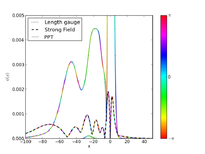
Figure 4: a) Full wavefunction propagated using exact propagator vs strong field propagator for initially quasistatic state b) Length gauge tunneling component propagated using exact propagator vs strong field propagator and PPT wavepacket. Whereas propagation of the full wavefunction fails completely for the strong field propagator, the tunneling component has comparable magnitude to that found using the exact propagator. The PPT wavepacket shows a markedly different magnitude and structure from the full strong field calculation. Lines show wavefunction magnitude, while color indicates phase.

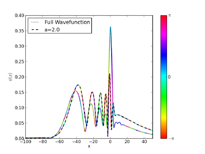
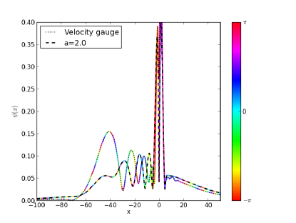
Figure 5: a) Full wavefunction propagated using exact propagator vs. propagator with modified short range potential b) Velocity gauge tunneling component propagated using exact propagator vs propagator with modified short range potential. Lines show wavefunction magnitude, while color indicates phase.

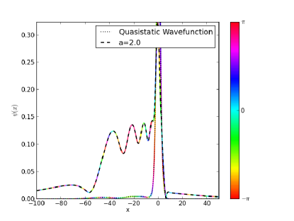
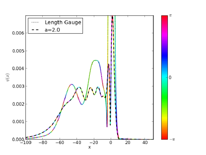
Figure 6: a) Full wavefunction propagated using exact propagator vs propagator with modified short range potential for initially quasistatic state b) Length gauge tunneling component propagated using exact propagator vs propagator with modified short range potential. Lines show wavefunction magnitude, while color indicates phase.

IV Conclusions

This paper has addressed the problem of strong field ionization from the perspective of the time dependent Schrödinger equation. Defining the tunneling component as that part of the wavefunction which differs from a precalculated bound state, we derived an inhomogeneous Schrödinger equation which governs its evolution. Our approach is manifestly gauge invariant, and we have exploited this invariance to shed light on an apparent gauge dependence which has long been puzzling in the context of the strong field approximation.

While our approach is formally equivalent to the full time dependent Schrödinger equation in the limit that an exact propagator is used, it eliminates a major error term when the propagation is approximate. It thus addressed a common problem in the theory of molecular strong field dynamics, where the computational methods necessary to describe the bound state may be prohibitively expensive to be used in a time dependent problem. Use of the inhomogeneous Schrödinger equation may thus represent a middle ground, allowing both the bound and the tunneling components to be treated using theoretical approaches which are most appropriate to the task.

References

- Becker and Faisal (2005) A. Becker and F. Faisal, Journal of Physics B: Atomic, Molecular and Optical Physics 38, R1 (2005).
- Ivanov et al. (2005) M. Ivanov, M. Spanner, and O. Smirnova, Journal of Modern Optics 52, 165 (2005).
- Smirnova et al. (2007) O. Smirnova, M. Spanner, and M. Ivanov, Journal of Modern Optics 54, 1019 (2007).
- Perelomov et al. (1966) A. Perelomov, V. Popov, and M. Terent’ev, Soviet Journal of Experimental and Theoretical Physics 23, 924 (1966).
- Smirnova et al. (2008) O. Smirnova, M. Spanner, and M. Ivanov, Physical Review A 77, 033407 (2008).
- Torlina and Smirnova (2012) L. Torlina and O. Smirnova, Physical Review A 86, 043408 (2012).
- Nest et al. (2005) M. Nest, T. Klamroth, and P. Saalfrank, The Journal of chemical physics 122, 124102 (2005).
- Caillat et al. (2005) J. Caillat, J. Zanghellini, M. Kitzler, O. Koch, W. Kreuzer, and A. Scrinzi, Physical review A 71, 012712 (2005).
- Zanghellini et al. (2004) J. Zanghellini, M. Kitzler, T. Brabec, and A. Scrinzi, Journal of Physics B: Atomic, Molecular and Optical Physics 37, 763 (2004).
- Moore et al. (2011a) L. Moore, M. Lysaght, L. Nikolopoulos, J. Parker, H. van der Hart, and K. Taylor, Journal of Modern Optics 58, 1132 (2011a).
- Lysaght et al. (2009) M. Lysaght, H. Van Der Hart, and P. Burke, Physical Review A 79, 053411 (2009).
- Moore et al. (2011b) L. Moore, M. Lysaght, J. Parker, H. van der Hart, and K. Taylor, Physical Review A 84, 061404 (2011b).
- Tao and Scrinzi (2012) L. Tao and A. Scrinzi, New Journal of Physics 14, 013021 (2012).
- Walters and Smirnova (2010) Z. Walters and O. Smirnova, Journal of Physics B: Atomic, Molecular and Optical Physics 43, 161002 (2010).
- Torlina et al. (2012) L. Torlina, M. Ivanov, Z. Walters, and O. Smirnova, Physical Review A 86, 043409 (2012).
- Spanner and Patchkovskii (2009) M. Spanner and S. Patchkovskii, Physical Review A 80, 063411 (2009).
- Becker and Milošević (2009) W. Becker and D. Milošević, Laser physics 19, 1621 (2009).
- Walters (2011) Z. Walters, Computer Physics Communications 182, 935 (2011).
- Scrinzi (2010) A. Scrinzi, Physical Review A 81, 053845 (2010).