Semi Markov model for market microstructure

Abstract

We introduce a new model for describing the fluctuations of a tick-by-tick single asset price. Our model is based on Markov renewal processes. We consider a point process associated to the timestamps of the price jumps, and marks associated to price increments. By modeling the marks with a suitable Markov chain, we can reproduce the strong mean-reversion of price returns known as microstructure noise. Moreover, by using Markov renewal processes, we can model the presence of spikes in intensity of market activity, i.e. the volatility clustering, and consider dependence between price increments and jump times. We also provide simple parametric and nonparametric statistical procedures for the estimation of our model. We obtain closed-form formula for the mean signature plot, and show the diffusive behavior of our model at large scale limit. We illustrate our results by numerical simulations, and find that our model is consistent with empirical data on the Euribor future.

Keywords: Microstructure noise, Markov renewal process, Signature plot, Scaling limit.

1 Introduction

The modeling of tick-by-tick asset price attracted a growing interest in the statistical and quantitative finance literature with the availability of high frequency data. It is basically split into two categories, according to the philosophy guiding the modeling:

(i) The macro-to-microscopic (or econometric) approach, see e.g. [12], [2], [14], interprets the observed price as a noisy representation of an unobserved one, typically assumed to be a continuous Itô semi-martingale: in this framework many important results exist on robust estimation of the realized volatility, but these models seem not tractable for dealing with high frequency trading problems and stochastic control techniques, mainly because the state variables are latent rather than observed.

(ii) The micro-to-macroscopic approach (e.g. [4], [3], [6], [1], [9]) uses point processes, in particular Hawkes processes, to describe the piecewise constant observed price, that moves on a discrete grid. In contrast with the macro-to-microscopic approach, these models do not rely on the arguable existence assumption of a fair or fundamental price, and focus on observable quantities, which makes the statistical estimation usually simpler. Moreover, these models are able to reproduce several well-known stylized facts on high frequency data, see e.g. [7], [5]:

• Microstructure noise: high-frequency returns are extremely anticorrelated, leading to a short-term mean reversion effect, which is mechanically explicable by the structure of the limit order book. This effect manifests through an increase of the realized volatility estimator (signature plot) when the observation frequency decreases from large to fine scales.

• Volatility clustering: markets alternates, independently of the intraday seasonality, between phases of high and low activity.

• At large scale, the price process displays a diffusion behaviour.

In this paper, we aim to provide a tractable model of tick-by-tick asset price for liquid assets in a limit order book with a constant bid-ask spread, in view of application to optimal high frequency trading problem, studied in the companion paper [10]. We start from a model-free description of the piecewise constant mid-price, i.e. the half of the best bid and best ask price, characterized by a marked point process $(T_{n},J_{n})_{n}$, where the timestamps $(T_{n})$ represent the jump times of the asset price associated to a counting process $(N_{t})$, and the marks $(J_{n})$ are the price increments. We then use a Markov renewal process (MRP) for modeling the marked point process. Markov renewal theory [13] is largely studied in reliability for describing failure of systems and machines, and one purpose of this paper is to show how it can be applied for market microstructure. By considering a suitable Markov chain modeling for $(J_{n})$, we are able to reproduce the mean-reversion of price returns, while allowing arbitrary jump size, i.e. the price can jump of more than one tick. Furthermore, the counting process $(N_{t})$, which may depend on the Markov chain, models the volatility clustering, i.e. the presence of spikes in the volatility of the stock price, and we also preserve a Brownian motion behaviour of the price process at macroscopic scales. Our MRP model is a rather simple but robust model, easy to understand, simulate and estimate, both parametrically and non-parametrically, based on i.i.d. sample data. An important feature of the MRP approach is the semi Markov property, meaning that the price process can be embedded into a Markov system with few additional and observable state variables. This will ensure the tractability of the model for applications to market making and statistical arbitrage.

The outline of the paper is the following. In Section 2, we describe the MRP model for the asset mid-price, and provides statistical estimation procedures. We show the simulation of the model, and the semi-Markov property of the price process. We also discuss the comparison of our model with Hawkes processes used for modeling asset prices and microstructure noise. Section 3 studies the diffusive limit of the asset price at macroscopic scale. In Section 4, we derive analytical formula for the mean signature plot, and compare with real data. Finally, Section 5 is devoted to a conclusion and extensions for future research.

2 Semi-Markov model

We describe the tick-by-tick fluctuation of a univariate stock price by means of a marked point process $(T_{n},J_{n})_{n\in\mathbb{N}}$. The increasing sequence $(T_{n})_{n}$ represents the jump (tick) times of the asset price, while the marks sequence $(J_{n})_{n}$ valued in the finite set

$$E=\{+1,-1,\ldots,+m,-m\}\subset\mathbb{Z}\setminus\{0\}$$

represents the price increments. Positive (resp. negative) mark means that price jumps upwards (resp. downwards). The continuous-time price process is a piecewise constant, pure jump process, given by

$$P_{t} = P_{0}+\sum_{n=1}^{N_{t}}J_{n},\;\;\;t\geq 0,$$ (2.1)

where $(N_{t})$ is the counting process associated to the tick times $(T_{n})_{n}$, i.e.

$$N_{t} = \inf\Big{\{}n:\sum_{k=1}^{n}T_{k}\leq t\Big{\}}$$

Here, we normalized the tick size (the minimum variation of the price) to $1$, and the asset price $P$ is considered e.g. as the last quotation for the mid-price, i.e. the mean between the best-bid and best-ask price. Let us mention that the continuous time dynamics (2.1) is a model-free description of a piecewise-constant price process in a market microstructure. We decouple the modeling on one hand of the clustering of trading activity via the point process $(N_{t})$, and on the other hand of the microstructure noise (mean-reversion of price return) via the random marks $(J_{n})_{n}$.

2.1 Price return modeling

We write the price return as

$$J_{n} = \hat{J}_{n}\,\xi_{n},\;\;\;n\geq 1,$$ (2.2)

where $\hat{J}_{n}$ $:=$ sign$(J_{n})$ valued in $\{+1,-1\}$ indicates whether the price jumps upwards or downwards, and $\xi_{n}$ $:=$ $|J_{n}|$ is the absolute size of the price increment. We consider that dependence of the price returns occurs through their direction, and we assume that only the current price direction will impact the next jump direction. Moreover, we assume that the absolute size of the price returns are independent and also independent of the direction of the jumps. Formally, this means that

• $(\hat{J}_{n})_{n}$ is an irreducible Markov chain with probability transition matrix

  $$\hat{Q} = \left(\begin{array}[]{cc}\frac{1+\alpha_{+}}{2}&\frac{1-\alpha_{+}}{2}\\ \frac{1-\alpha_{-}}{2}&\frac{1+\alpha_{-}}{2}\end{array}\right)$$ (2.5)

  with $\alpha_{+},\alpha_{-}$ $\in$ $[-1,1)$.

• $(\xi_{n})_{n}$ is an i.i.d. sequence valued in $\{1,\ldots,m\}$, independent of $(\hat{J}_{n})$, with distribution law: $p_{i}$ $=$ $\mathbb{P}[\xi_{n}=i]$ $\in$ $(0,1)$, $i$ $=$ $1,\ldots,m$.

In this case, $(J_{n})$ is an irreducible Markov chain with probability transition matrix given by:

$$Q = \left(\begin{array}[]{ccc}p_{1}\hat{Q}&\ldots&p_{m}\hat{Q}\\ \vdots&\ddots&\vdots\\ p_{1}\hat{Q}&\ldots&p_{m}\hat{Q}\end{array}\right).$$ (2.9)

We could model in general $(J_{n})_{n}$ as a Markov chain with transition matrix $Q$ $=$ $(q_{ij})$ involving $2m(2m-1)$ parameters, while under the above assumption, the matrix $Q$ in (2.9) involves only $m+1$ parameters to be estimated. Actually, on real data, we often observe that the number of consecutive downward and consecutive upward jumps are roughly equal. We shall then consider the symmetric case where

$$\alpha_{+} = \alpha_{-}\;=:\;\alpha.$$ (2.10)

In this case, we have a nice interpretation of the parameter $\alpha$ $\in$ $[-1,1)$.

Lemma 2.1

In the symmetric case, the invariant distribution of the Markov chain $(\hat{J}_{n})_{n}$ is $\hat{\pi}$ $=$ $(\frac{1}{2},\frac{1}{2})$, and the invariant distribution of $(J_{n})_{n}$ is $\pi$ $=$ $(p_{1}\hat{\pi},\ldots,p_{m}\hat{\pi})$. Moreoever, we have:

$$\alpha = {\rm corr}_{\pi}\big{(}\hat{J}_{n},\hat{J}_{n-1}\big{)},\;\;\;\forall n\geq 1,$$ (2.11)

where ${\rm corr}_{\pi}$ denotes the correlation under the stationary probability $\mathbb{P}_{\pi}$ starting from the initial distribution $\pi$.

Proof. We easily check that under the symmetric case, $\hat{\pi}\hat{Q}$ $=$ $\hat{\pi}$ for $\hat{\pi}$ $=$ $(1/2,1/2)$, which means that $\hat{\pi}$ is the invariant distribution of the Markov chain $(\hat{J}_{n})_{n}$. Consequently, $\pi$ $=$ $(p_{1}\hat{\pi},\ldots,p_{m}\hat{\pi})$ satisfies $\pi Q$ $=$ $\pi$, i.e. $\pi$ is the invariant distribution of $(J_{n})_{n}$, and so under $\mathbb{P}_{\pi}$, $(\hat{J}_{n})_{n}$ (resp. $(J_{n})_{n}$) is distributed according to $\hat{\pi}$ (resp. $\pi$). Therefore, $\mathbb{E}_{\pi}[\hat{J}_{n}]$ $=$ $0$ and $\mbox{Var}_{\pi}[\hat{J}_{n}]$ $=$ $1$. We also have for all $n$ $\geq$ $1$, by definition of $\hat{Q}$:

$$\mathbb{E}_{\pi}\big{[}\hat{J}_{n}\hat{J}_{n-1}\big{]} = \mathbb{E}_{\pi}\Big{[}\frac{1+\alpha}{2}\big{(}\hat{J}_{n-1}\big{)}^{2}-\frac{1-\alpha}{2}\big{(}\hat{J}_{n-1}\big{)}^{2}\Big{]}\;=\;\alpha,$$

which proves the relation (2.11) for $\alpha$. $\Box$

Lemma 2.1 provides a direct interpretation of the parameter $\alpha$ as the correlation between two consecutive price return directions. The case $\alpha$ $=$ $0$ means that price returns are independent, while $\alpha$ $<$ $0$ (resp. $\alpha$ $>$ $0$) corresponds to a mean-reversion (resp. trend) of price return.

We also have another equivalent formulation of the Markov chain, whose proof is trivial and left to the reader.

Lemma 2.2

In the symmetric case, the Markov chain $(\hat{J}_{n})_{n}$ can be written as:

$$\hat{J}_{n} = \hat{J}_{n-1}B_{n},\;\;\;n\geq 1,$$

where $(B_{n})_{n}$ is a sequence of i.i.d. random variables with Bernoulli distribution on $\{+1,-1\}$, and parameter $(1+\alpha)/2$, i.e. of mean $\mathbb{E}[B_{n}]$ $=$ $\alpha$. The price increment Markov chain $(J_{n})_{n}$ can also be written in an explicit induction form as:

$$J_{n} = \hat{J}_{n-1}\zeta_{n},$$ (2.12)

where $(\zeta_{n})_{n}$ is a sequence of i.i.d. random variables valued in $E$ $=$ $\{+1,-1,\ldots,+m,-m\}$, and with distribution: $\mathbb{P}[\zeta_{n}=k]$ $=$ $p_{k}(1+\mbox{sign}(k)\alpha)/2$.

The above Lemma is useful for an efficient estimation of $\alpha$. Actually, by the strong law of large numbers, we have a consistent estimator of $\alpha$:

$$\hat{\alpha}^{(n)} = \frac{1}{n}\sum_{k=1}^{n}\frac{\hat{J}_{k}}{\hat{J}_{k-1}}\;=\;\frac{1}{n}\sum_{k=1}^{n}\hat{J}_{k}\hat{J}_{k-1}.$$

The variance of this estimator is known, equal to $1/n$, so that this estimator is efficient and we have a confidence interval from the central limit theorem:

$$\sqrt{n}(\hat{\alpha}^{(n)}-\alpha) \stackrel{{\scriptstyle(d)}}{{\longrightarrow}} {\cal N}(0,1),\;\;\;\mbox{ as }n\rightarrow\infty.$$

The estimated parameter for the chosen dataset is $\hat{\alpha}$ $=$ $-87.5\%$, which shows as expected a strong anticorrelation of price returns. In the case of several tick jumps $m$ $>$ $1$, the probability $p_{i}$ $=$ $\mathbb{P}[\xi_{n}=i]$ may be estimated from the classical empirical frequency:

$$\hat{p}_{i}^{(n)}=\frac{1}{n}\sum_{k=1}^{n}1_{\xi_{k}=i},\;\;\;i=1,\ldots,m$$

2.2 Tick times modeling

In order to describe volatility clustering, we look for a counting process $(N_{t})$ with an intensity increasing every time the price jumps, and decaying with time. We propose a modeling via Markov renewal process.

Let us denote by $S_{n}$ $=$ $T_{n}-T_{n-1}$, $n$ $\geq$ $1$, the inter-arrival times associated to $(N_{t})$. We assume that conditionally on the jump marks $(J_{n})_{n}$, $(S_{n})_{n}$ is an independent sequence of positive random times, with distribution depending on the current and next jump mark:

$$F_{ij}(t) = \mathbb{P}[S_{n+1}\leq t\;|\;J_{n}=i,J_{n+1}=j],\;\;\;(i,j)\in E.$$

We then say that $(T_{n},J_{n})_{n}$ is a Markov Renewal Process (MRP) with transition kernel:

$$\mathbb{P}[J_{n+1}=j,S_{n+1}\leq t\;|\;J_{n}=i] = q_{ij}F_{ij}(t),\;\;\;(i,j)\in E.$$

In the particular case where $F_{ij}$ does not depend on $i,j$, the point process $(N_{t})$ is independent of $(J_{n})$, and called a renewal process, Moreover, if $F$ is the exponential distribution, $N$ is a Poisson process. Here, we allow in general dependency between jump marks and renewal times, and we refer to the symmetric case when $F_{ij}$ depends only on the sign of $ij$, by setting:

$$F_{+}(t)\;=\;F_{ij}(t),\;\;\;\mbox{ if }\;ij>0, F_{-}(t)\;=\;F_{ij}(t),\;\;\;\mbox{ if }\;ij<0.$$ (2.13)

In other words, $F_{+}$ (resp. $F_{-}$) is the distribution function of inter-arrival times given two consecutive jumps in the same (resp. opposite) direction, called trend (resp. mean-reverting) case. Let us also introduce the marked hazard function:

$$h_{ij}(t) = \lim_{\delta\downarrow 0}\frac{1}{\delta}\mathbb{P}[t\leq S_{n+1}\leq t+\delta,\;J_{n+1}=j\;|\;S_{n}\geq t,\;J_{n}=i],\;\;\;t\geq 0,$$ (2.14)

for $i,j$ $\in$ $E$, which represents the instantaneous probability that there will be a jump with mark $j$, given that there were no jump during the elapsed time $t$, and the current mark is $i$. By assuming that the distributions $F_{ij}$ of the renewal times $S_{n}$ admit a density $f_{ij}$, we may write $h_{ij}$ as:

$$h_{ij}(t) = q_{ij}\frac{f_{ij}(t)}{1-H_{i}(t)}=:q_{ij}\lambda_{ij},$$

where

$$H_{i}(t) = \mathbb{P}[S_{n+1}\leq t\;|\;J_{n}=i]\;=\;\sum_{j\in E}q_{ij}F_{ij}(t),$$

is the conditional distribution of the renewal time in state $i$. In the symmetric case (2.10), (2.13), we have

$$h_{ij}(t) = p_{j}\Big{(}\frac{1+{\rm sign}(ij)\alpha}{2}\Big{)}\lambda_{{\rm sign}(ij)}(t),$$

with jump intensity

$$\lambda_{\pm}(t) = \frac{f_{\pm}(t)}{1-F(t)},$$ (2.15)

where $f_{\pm}$ is the density of $F_{\pm}$, and

$$F(t) = \frac{1+\alpha}{2}F_{+}(t)+\frac{1-\alpha}{2}F_{-}(t).$$

Markov renewal processes are used in many applications, especially in reliability. Classical examples of renewal distribution functions are the ones corresponding to the Gamma and Weibull distribution, with density given by:

$$f_{Gam}(t)\;=\;\frac{t^{\beta-1}e^{-t/\theta}}{\Gamma(\beta)\theta^{\beta}} \;\;\;f_{Wei}(t)\;=\;\frac{\beta}{\theta}\Big{(}\frac{t}{\theta}\Big{)}^{\beta-1}e^{-\beta t/\theta}$$

where $\beta$ $>$ $0$, and $\theta$ $>$ $0$ are the shape and scale parameters, and $\Gamma$ (resp. $\Gamma_{t}$) is the Gamma (resp. lower incomplete Gamma) function:

$$\Gamma(\beta)\;=\;\int_{0}^{\infty}s^{\beta-1}e^{-s}ds,\;\; \;\;\Gamma_{t}(\beta)\;=\;\int_{0}^{t}s^{\beta-1}e^{-s}ds,$$ (2.16)

2.3 Statistical procedures

We design simple statistical procedures for the estimation of the distribution and jump intensities of the renewal times. Over an observation period, pick a subsample of i.i.d. data:

$$\{S_{k}=T_{k}-T_{k-1}:k\;s.t.\;J_{k-1}=i,\;J_{k}=j\},$$

and set:

$$I_{ij} = \#\{k\;s.t.\;J_{k-1}=i,\;J_{k}=j\}$$

$$I_{i} = \#\{k\;s.t.\;J_{k-1}=i\},$$

with cardinality respectively $n_{ij}$ and $n_{i}$. In the symmetric case, we also denote by

$$I_{\pm} = \#\{k\;s.t.\;sign(J_{k-1}J_{k})=\pm\},$$

with cardinality $n_{\pm}$. We describe both parametric and nonparametric estimation.

$\bullet$ Parametric estimation

We discuss the parametric estimation of the distribution $F_{ij}$ of the renewal times when considering Gamma or Weibull distributions with shape and scale parameters $\beta_{ij}$, $\theta_{ij}$. We can indeed consider the Maximum Likelihood Estimator (MLE) $(\hat{\beta}_{ij},\hat{\theta}_{ij})$, which are solution to the equations:

$$\ln\hat{\beta}_{ij}-\frac{\Gamma^{\prime}(\hat{\beta}_{ij})}{\Gamma(\hat{\beta}_{ij})} = \ln\Big{(}\frac{1}{n_{ij}}\sum_{k=1}^{n_{ij}}S_{k}\Big{)}-\frac{1}{N}\sum_{k=1}^{n_{ij}}\ln S_{k}$$

$$\hat{\theta}_{ij} = \frac{1}{\hat{\beta}_{ij}}\bar{S}_{n_{ij}},\;\;\;\mbox{ with }\;\bar{S}_{n_{ij}}\;:=\;\frac{1}{n_{ij}}\sum_{k=1}^{n_{ij}}S_{k}$$

There is no closed-form solution for $\hat{\beta}_{ij}$, which can be obtained numerically e.g. by Newton method. Alternatively, since the first two moments of the Gamma distribution $S$ $\leadsto$ $\Gamma(\beta,\theta)$ are explicitly given in terms of the shape and scale parameters, namely:

$$\beta\;=\;\frac{\big{(}\mathbb{E}[S]\big{)}^{2}}{{\rm Var}[S]},\;\;\; \;\;\;\frac{1}{\theta}\;=\;\frac{\mathbb{E}[S]}{{\rm Var}[S]},$$ (2.17)

we can estimate $\beta_{ij}$ and $\theta_{ij}$ by moment matching method, i.e. by replacing in (2.17) the mean and variance by their empirical estimators, which leads to:

$$\tilde{\beta}_{ij}\;=\;\frac{n_{ij}\bar{S}_{n_{ij}}^{2}}{\displaystyle\sum_{k=1}^{n_{ij}}(S_{k}-\bar{S}_{n_{ij}})^{2}},\;\; \;\;\frac{1}{\tilde{\theta}_{ij}}\;=\;\frac{n_{ij}\bar{S}_{n_{ij}}}{\displaystyle\sum_{k=1}^{n_{ij}}(S_{k}-\bar{S}_{n_{ij}})^{2}}.$$

We performed this parametric estimation method for the Euribor on the year 2010, from 10h to 14h, with one tick jump, and obtain the following estimates in Table 1.

i	j	shape	scale
+1	+1	0.27651097	2187
-1	-1	0.2806104	2565.371
+1	-1	0.07442401	1606.308
-1	+1	0.06840708	1508.155

Table 1: Parameter estimates for the renewal times of a Gamma distribution

We observed that the shape and scale parameters depend on the product $ij$ rather than on $i$ and $j$ separately. In other words, the distribution of the renewal times are symmetric in the sense of (2.13). Hence, we performed again in Table 2. the parametric estimation $(\tilde{\beta}_{+},\tilde{\theta}_{+})$ and $(\tilde{\beta}_{-},\tilde{\theta}_{-})$ for the shape and scale parameters by distinguishing only samples for $ij$ $=$ $1$ (the trend case) and $ij$ $=$ $-1$ (the mean-reverting case). We also provide in Figure 1 graphical tests of the goodness-of-fit for our estimation results. The estimated value $\tilde{\beta}_{+}$, and $\tilde{\beta}_{-}$ $<$ $1$ for the shape parameters, can be interpreted when considering the hazard rate function of $S_{n+1}$ given current and next marks:

$$\hat{\lambda}_{\pm}(t) := \lim_{\delta\downarrow 0}\frac{1}{\delta}\mathbb{P}[t\leq S_{n+1}\leq t+\delta|S_{n}\geq t,{\rm sign}(J_{n}J_{n+1})=\pm]$$

$$= \frac{f_{\pm}(t)}{1-F_{\pm}(t)},\;\;\;t\geq 0,$$

when $F_{\pm}$ admits a density $f_{\pm}$ (Notice that $\hat{\lambda}_{\pm}$ differs from $\lambda_{\pm}$). $\hat{\lambda}_{+}(t)$ (resp. $\hat{\lambda}_{-}(t))$ is the instantaneous probability of price jump given that there were no jump during an elapsed time $t$, and the current and next jump are in the same (resp. opposite) direction. For the Gamma distribution with shape and scale parameters $(\beta,\theta)$, the hazard rate function is given by:

$$\hat{\lambda}_{Gam}(t) = \frac{1}{\theta}\frac{\Big{(}\frac{t}{\theta}\Big{)}^{\beta-1}e^{-t/\theta}}{\Gamma(\beta)-\Gamma_{t/\theta}(\beta)},\;\;\;$$

and is decreasing in time if and only if the shape parameter $\beta$ $<$ $1$, which means that the more the time passes, the less is the probability that an event occurs. Therefore, the estimated values $\hat{\beta}_{+}$, and $\tilde{\beta}_{-}$ $<$ $1$ are consistent with the volatility clustering: when a jump occurs, the probability of another jump in a short period is high, but if the event does not take place soon, then the price is likely to stabilize. Using this modeling, a long period of constant price corresponds to a renewal time in distribution tail. On the contrary, since renewal times are likely to be small when $\beta<1$, most of the jumps will be extremely close. We also notice that the parameters in the trend and mean-reverting case differ significantly. This can be explained as follows: trends, i.e. two consecutive jumps in the same direction, are extremely rare (recall that $\alpha\approx-90\%$), since, in order to take place, market orders either have to clear two walls of liquidity or there must be a big number of cancellations. Since these events are caused by specific market dynamic, it is not surprising that their renewal law differ from the mean-reverting case.

i j	shape	scale
+1 (trend)	0.276225	2397.219
-1 (mean-reverting)	0.07132677	1561.593

Table 2: Parameter estimates in the trend and mean-reverting case

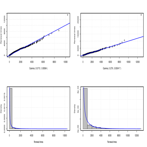
Figure 1: QQ plot and histogram of $F_{-}$(left) and $F_{+}$ (right). Euribor3m, 2010, 10h-14h.

$\bullet$ Non parametric estimation

Since the renewal times form an i.i.d. sequence, we are able to perform a non parametric estimation by kernel method of the density $f_{ij}$ and the jump intensity. We recall the smooth kernel method for the density estimation, and, in a similar way, we will give the one for $h_{\ij}$ and $\lambda_{ij}$. Let us start with the empirical histogram of the density, which is constructed as follows. For every collection of breaks

$$\{0<t_{1}<...<t_{M}\leq\infty\},\;\;\;\delta_{r}\;:=\;t_{r+1}-t_{r}$$

we bin the sample $(S_{k}=T_{k}-T_{k-1})_{k=1,\ldots,n}$ and define the empirical histogram of $f_{ij}$ as:

$$f^{hst}_{ij}\,(t_{r}) = \frac{1}{\delta_{r}}\frac{\#\{k\in I_{ij}\;|\;t_{r}\leq S_{k}<t_{r+1}\}}{n_{ij}}.$$

By the strong law of large numbers, when $n_{ij}\rightarrow\infty$, this estimator converges to

$$\frac{1}{\delta_{r}}\mathbb{P}\left[t_{r}\leq S_{k}<t_{r+1}\right],$$

which is a first order approximation of $f_{ij}(t_{r})$. Anyway, this estimator depends on the choice of the binning, which has not necessarily small (nor equal) $\delta_{r}$’s. The corresponding non parametric (smooth kernel) estimator of the density is given by a convolution method:

$$f^{np}_{ij}(t) = \frac{1}{n_{ij}}\sum_{k\in I_{ij}}\,K_{b}(t-S_{k}),$$

where $K_{b}(x)$ is a smoothing scaled kernel with bandwidth $b$. In our example we have chosen the Gaussian one, given by the density of the normal law of mean $0$ and variance $b^{2}$. In practice, many softwares provide already optimized version of non-parametric estimation of the density, with automatic choice of the bandwidth and of the kernel (here Gaussian). For example in $R$, this reduces to the function density, applied to the sample $\{S_{k}\;|\;k\in I_{ij}\}$. In the symmetric case, the histogram reduces to:

$$f^{hst}_{\pm}\,(t_{r}) = \frac{1}{\delta_{r}}\frac{\#\{k\in I_{\pm}\;|\;t_{r}\leq S_{k}<t_{r+1}\}}{n_{\pm}},$$

while the kernel estimator is given by:

$$f^{np}_{\pm}(t) = \frac{1}{n_{\pm}}\sum_{k\in I_{\pm}}\,K_{b}(t-S_{k}).$$

Figure 2 shows the result obtained for the kernel estimation of $f_{\pm}(t)$, compared to the corresponding histogram. The non parametric estimation confirms the decreasing form of both of the densities, whose interpetation is that most of the jump of the stock price takes place in a short period of time (less than second), even though some renewal times can go to hours.

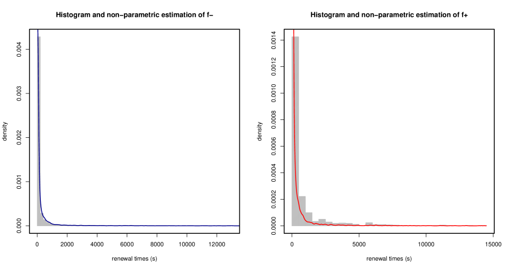
Figure 2: Nonparametric estimation of the densities $f_{+}$ and $f_{-}$

We use similar technique to estimate the marked hazard function $h_{ij}$ defined in (2.14). By writing

$$h_{ij}(t) = \lim_{\delta\rightarrow 0}\frac{1}{\delta}\frac{\mathbb{P}\left[t\leq S_{k}<t+\delta,\;J_{k}=j\;|\;J_{k-1}=i\right]}{\mathbb{P}\left[S_{k}\geq s\;|\;J_{k-1}=i\right]},$$

we can define the empirical histogram of $h_{ij}$ as

$$h^{hst}_{ij}(t_{r}) = \frac{1}{\delta_{r}}\frac{\#\{k\in I_{ij}\;|\;t_{r}\leq S_{k}<t_{r}+\delta\}}{\#\{k\in I_{i}\;|\;S_{k}\geq t_{r}\}},$$

and the associated smooth kernel estimator by

$$h^{np}_{ij}(t) = \sum_{k\in I_{ij}}\,K_{b}(t-S_{k})\,\frac{1}{\#\{k\in I_{i}\;|\;S_{k}\geq t\}}.$$

Notice that this nonparametric estimator is factorized as

$$h^{np}_{ij}(t) = \left(\frac{n_{ij}}{n_{i}}\right)\left(\frac{n_{i}}{n_{ij}}h^{np}_{ij}(t)\right)$$

where $\frac{n_{ij}}{n_{i}}$ is the estimator of $q_{ij}$ and $\frac{n_{i}}{n_{ij}}h^{np}_{ij}(t)$ is the kernel estimator of the jump intensity $\lambda_{ij}(t)$ $=$ $\frac{f_{ij}(t)}{1-H_{i}(t)}$. Thus, we can either estimate $\lambda_{ij}$ and multiply by the estimator of $q_{ij}$ to obtain $h_{ij}$ or vice versa, obtaining the same estimators. In the symmetric case, we have:

$$h^{hst}_{\pm}(t_{r}) = \frac{1}{\delta_{r}}\frac{\#\{k\in I_{\pm}\;|\;t_{r}\leq S_{k}<t_{r}+\delta\}}{\#\{k\;|\;S_{k}\geq t_{r}\}},$$

while

$$h^{np}_{\pm}(t) = \sum_{k\in I_{\pm}}\,K_{b}(t-S_{k})\,\frac{1}{\#\{k\;|\;S_{k}\geq t\}}.$$

Figure 3 shows the result obtained for $\lambda_{\pm}$, compared to the corresponding histogram. The interpretation is the following: immediately after a jump the price is in an unstable condition, which will probably leads it to jump again soon. If it does not happen, the price gains in stability with time, and the probability of a jump becomes smaller and smaller. Moreover, due to mean-reversion of price returns, the intensity of consecutive jumps in the opposite direction is larger than in the same direction, which explains the higher value of $\lambda_{-}$ compared to $\lambda_{+}$.

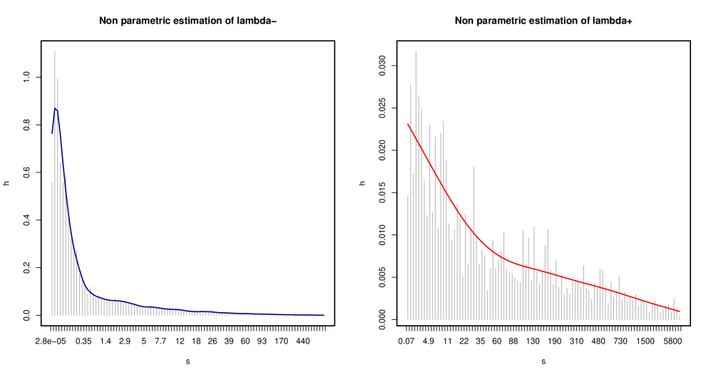
Figure 3: Nonparametric estimation of the jump intensities $\lambda_{+}$ and $\lambda_{-}$

2.4 Price simulation

The simulation of the price process (2.1) with a Markov renewal model is quite simple, much easier than any other point process modeling microstructure noise. This would allow the user, even when $N_{t}$ is better fit by a more complex point process, to have a quick proxy for its price simulation. Choose a starting price $P_{0}$ at initial time $T_{0}$.

Initialization step:

• Set $\hat{P}_{0}=P_{0}$

• draw $J_{0}$ from initial (e.g. stationary) law $\pi$

Inductive step:

$k-1$ $\rightarrow$ $k$ (next price and next timestamp)

• Draw $J_{k}$ according to the probability transition, and set $\hat{P}_{k}$ $=$ $\hat{P}_{k-1}$ $+$ $J_{k}$.

• Draw $S_{k}$ $\leadsto$ $F_{J_{k-1}J_{k}}$, and set $T_{k}$ $=$ $T_{k-1}+S_{k}$.

Once $(T_{k},\hat{P}_{k})_{k\in\mathbb{N}}$ is known, the price process is given by the piecewise constant process:

$$P_{t} = \hat{P}_{k},\;\;\;T_{k}\leq t<T_{k+1}.$$

We show in Figure 4 some simulated trajectories of the price process based on the estimated parameters of the Euribor3m.

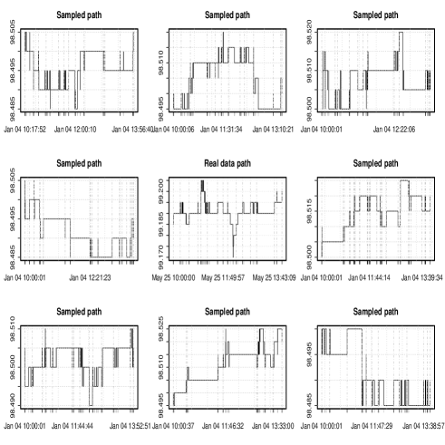
Figure 4: Simulation of $9$ trajectories of the Euribor with estimated parameters on empirical data

2.5 Semi-Markov property

Let us define the pure jump process,

$$I_{t}=J_{N_{t}}$$ (2.18)

which represents the last price increment. Then, $I$ is a semi-Markov process in the sense that the pair $(I_{t},S_{t})$ is a Markov process, where

$$S_{t} = t-T_{n},\;\;T_{n}\leq t<T_{n+1},$$

is the time spent from the last jump price. Moreover, the price process $(P_{t})$ is embedded in a Markov process with three observable state variables: $(P_{t},I_{t},S_{t})$ is a Markov process with infinitesimal generator:

$${\cal L}\varphi(p,i,s) = \displaystyle\frac{\partial\varphi}{\partial s}\;+\;\sum_{j\in E}h_{ij}(s)[\varphi(p+j,j,0)-\varphi(p,i,s)],$$

which is written in the symmetric case (2.10) and (2.13) as

$${\cal L}\varphi(p,i,s) = \displaystyle\frac{\partial\varphi}{\partial s}\;+\;\lambda_{+}(s)\Big{(}\frac{1+\alpha}{2}\Big{)}\sum_{j=1}^{m}p_{j}[\varphi(p+{\rm sign}(i)j,{\rm sign}(i)j,0)-\varphi(p,i,s)]$$

$$\;\;\;\;+\;\lambda_{-}(s)\Big{(}\frac{1-\alpha}{2}\Big{)}\sum_{j=1}^{m}p_{j}[\varphi(p-{\rm sign}(i)j,-{\rm sign}(i)j,0)-\varphi(p,i,s)],$$

where $\lambda_{\pm}$ is the jump intensity defined in (2.15).

2.6 Comparison with respect to Hawkes processes

In a recent work [3] (see also [9]), the authors consider a tick-by-tick model for asset price by means of cross-exciting Hawkes processes. More precisely, the stock price jumps by one tick according to the dynamics:

$$P_{t} = N_{t}^{+}-N_{t}^{-},$$ (2.19)

where $N^{\pm}$ is a point process corresponding to the number of upward and downward jumps, with coupling stochastic intensities:

$$\lambda_{t}^{\pm} = \lambda_{\infty}+\int_{-\infty}^{t}\varphi(t-u)dN_{u}^{\mp},$$ (2.20)

where $\lambda_{\infty}$ $>$ $0$ is an exogenous constant intensity, and $\varphi$ is a positive decay kernel. This model, which takes into account in the intensity the whole past of the price process, provides a better good-fit of intraday data than the MRP approach, and can be easily extended to the multivariate asset price case. However, it is limited to unitary jump size, and presents some drawbacks especially in view of applications to trading optimization problem. The price process in (2.19)-(2.20) is embedded into a Markovian framework only for the case of exponential decay kernel, i.e. for

$$\varphi(t) = \gamma e^{-\beta t}1_{\mathbb{R}_{+}}(t),$$

with $0$ $<$ $\gamma$ $<$ $\beta$. In this case, the Markov price system consists of $P$ together with the stochastic intensities $(\lambda^{+},\lambda^{-})$. But in contrast with the MRP approach, the additional state variables $(\lambda^{+},\lambda^{-})$ are not directly observable, and have to be computed from their dynamics (2.20), which requires a “precise” estimation of the three parameters $\lambda_{\infty}$, $\gamma$, and $\beta$. In that sense, the MRP approach is more robust than the Hawkes approach when dealing with Markov optimization problem. Notice also that in the MRP approach, we can deal not only with parametric forms of the renewal distributions (which involves only two parameters for the usual Gamma and Weibull laws), but also with non parametric form of the renewal distributions, and so of the jump intensities. Simulation and estimation in MRP model are simple since they are essentially based on (conditional) i.i.d. sequence of random variables, with the counterpart that MRP model can not reproduce the correlation between inter-arrival jump times as in Hawkes model.

We finally mention that one can use a combination of Hawkes process and semi Markov model by considering a counting process $N_{t}$ associated to the jump times $(T_{n})$, independent of the price return $(J_{n})$, and with stochastic intensity

$$\lambda_{t} = \lambda_{\infty}+\gamma\int_{0}^{t}e^{-\beta(t-u)}dN_{u},$$ (2.21)

with $\lambda_{\infty}$ $>$ $0$, and $0<\gamma<\beta$. In this case, the pair $(I_{t},\lambda_{t})$ is a Markov process, and $(P_{t},I_{t},\lambda_{t})$ is a Markov process with infinitesimal generator:

$${\cal L}\varphi(p,i,\ell) = \beta(\mu-\ell)\displaystyle\frac{\partial\varphi}{\partial\ell}\;+\;\ell\sum_{j\in E}q_{ij}[\varphi(p+j,j,\ell+\gamma)-\varphi(p,i,\ell)],$$

which is written in the symmetric case (2.10) as:

$${\cal L}\varphi(p,i,\ell) = \beta(\mu-\ell)\displaystyle\frac{\partial\varphi}{\partial\ell}$$

$$\;\;\;+\;\ell\Big{(}\frac{1+\alpha}{2}\Big{)}\sum_{j=1}^{m}p_{j}[\varphi(p+{\rm sign}(i)j,{\rm sign}(i)j,\ell+\gamma)-\varphi(p,i,\ell)]$$

$$\;\;\;+\;\ell\Big{(}\frac{1-\alpha}{2}\Big{)}\sum_{j=1}^{m}p_{j}[\varphi(p-{\rm sign}(i)j,-{\rm sign}(i)j,\ell+\gamma)-\varphi(p,i,\ell)].$$

3 Scaling limit

We now study the large scale limit of the price process constructed from our Markov renewal model. We consider the symmetric case (2.10) and (2.13), and denote by

$$F(t) = \frac{1+\alpha}{2}F_{+}(t)+\frac{1-\alpha}{2}F_{-}(t),$$

the distribution function of the sojourn time $S_{n}$. We assume that the mean sojourn time is finite:

$$\bar{\mu} = \int_{0}^{\infty}t\;dF(t)\;<\;\infty,\;\;\;\mbox{ and we set }\;\bar{\lambda}=\frac{1}{\bar{\mu}}.$$

By classical regenerative arguments, it is known (see [11]) that the Markov renewal process obeys a strong law of large numbers, which means the long run stability of price process:

$$\frac{P_{t}}{t} \longrightarrow c,\;\;\;a.s.$$

when $t$ goes to infinity, with a limiting constant $c$ given by:

$$c = \frac{1}{\bar{\mu}}\sum_{i,j\in E}\pi_{i}\,q_{ij}\,j,$$

where $E$ $=$ $\{1,-1,\ldots,m,-m\}$, $\bar{\mu}_{ij}$ $=$ $\int_{0}^{\infty}tdF_{ij}(t)$, $Q$ $=$ $(q_{ij})$ is the transition matrix (2.9) of the embedded Markov chain $(J_{n})_{n}$, and $\pi$ $=$ $(\pi_{i})$ is the invariant distribution of $(J_{n})_{n}$. In the symmetric case (2.10) and (2.13), we have $q_{ij}$ $=$ $p_{|i|}(1+{\rm sign}(j)\alpha)/2$, $\pi_{i}$ $=$ $p_{|i|}/2$, and so $c$ $=$ $0$. We next define the normalized price process:

$$P^{(T)}_{t} = \frac{P_{tT}}{\sqrt{T}},\;\;\;t\in[0,1],$$

and address the macroscopic limit of $P^{(T)}$ at large scale limit $T$ $\rightarrow$ $\infty$. From the functional central limit theorem for Markov renewal process, we obtain the large scale diffusive behavior of price process.

Proposition 3.1

$$\lim_{T\rightarrow\infty}P^{(T)} \stackrel{{\scriptstyle(d)}}{{=}} \sigma_{{}_{\infty}}W,$$

where $W$ $=$ $(W_{t})_{t\in[0,1]}$ is a standard Brownian motion, and $\sigma_{{}_{\infty}}$, the macroscopic variance, is explicitly given by

$$\sigma_{{}_{\infty}}^{2} = \bar{\lambda}\Big{[}{\rm Var}(\xi_{n})+\big{(}\mathbb{E}[\xi_{n}]\big{)}^{2}\;\frac{1+\alpha}{1-\alpha}\Big{]}.$$ (3.1)

Proof. From [11], we know that a functional central limit theorem holds for Markov renewal process so that

$$P^{(T)} \stackrel{{\scriptstyle(d)}}{{\rightarrow}} \sigma_{{}_{\infty}}W$$

when $T$ goes to infinity (here $\stackrel{{\scriptstyle(d)}}{{\rightarrow}}$ means convergence in distribution), where $\sigma_{{}_{\infty}}$ is given by $\sigma_{{}_{\infty}}^{2}$ $=$ $\bar{\lambda}\tilde{\sigma}_{{}_{\infty}}^{2}$ with $\bar{\lambda}$ $=$ $1/\bar{\mu}$, and

$$\tilde{\sigma}_{{}_{\infty}}^{2} = \sum_{i,j\in E}\pi_{i}q_{ij}H_{ij}^{2},$$

with

$$H_{ij} = j+g_{j}-g_{i}$$

$$g=(g_{i})_{i} = (I_{2m}-Q+\Pi)^{-1}b$$

$$b=(b_{i}),\;b_{i} = \sum_{j\in E}Q_{ij}j,$$

and $\Pi$ is the matrix defined by $\Pi_{ij}$ $=$ $\pi_{j}$. In the symmetric case (2.10), a straightforward calculation shows that

$$b_{i} = {\rm sign}(i)\alpha\sum_{j=1}^{m}jp_{j}\;=\;{\rm sign}(i)\alpha\mathbb{E}[\xi_{n}],$$

and then

$$g_{i} = {\rm sign}(i)\frac{\alpha}{1-\alpha}\mathbb{E}[\xi_{n}],\;\;\;i\in E=\{1,-1,\ldots,m,-m\}.$$

Thus,

$$H_{ij} = \left\{\begin{array}[]{cc}j&\mbox{ if }ij>0\\ j+\frac{2\alpha}{1-\alpha}\mathbb{E}[\xi_{n}]&\mbox{ if }j>0,i<0\\ j-\frac{2\alpha}{1-\alpha}\mathbb{E}[\xi_{n}]&\mbox{ if }j<0,i>0.\end{array}\right.$$

Therefore, a direct calculation yields

$$\tilde{\sigma}_{{}_{\infty}}^{2} = \sum_{j=1}^{m}j^{2}p_{j}+\frac{2\alpha}{1-\alpha}\big{(}\mathbb{E}[\xi_{n}]\big{)}^{2}$$

$$= {\rm Var}(\xi_{n})+\big{(}\mathbb{E}[\xi_{n}]\big{)}^{2}\;\frac{1+\alpha}{1-\alpha}.$$

$\Box$

4 Mean Signature plot

In this section, we aim to provide through our Markov renewal model a quantitative justification of the signature plot effect, described in the introduction. We consider the symmetric and stationary case, i.e.:

(H)

• The price return $(J_{n})_{n}$ is given by (2.2) with a probability transition matrix $\hat{Q}$ for $(\hat{J}_{n})_{n}$ $=$ $({\rm sign}(J_{n}))_{n}$ in the form:

  $$\hat{Q} = \left(\begin{array}[]{cc}\frac{1+\alpha}{2}&\frac{1-\alpha}{2}\\ \frac{1-\alpha}{2}&\frac{1+\alpha}{2}\end{array}\right)$$

  for some $\alpha$ $\in$ $[-1,1)$ .

• $(N_{t})$ is a delayed renewal process: for $n$ $\geq$ $1$, $S_{n}$ has distribution function $F$ (independent of $i,j$), with finite mean $\bar{\mu}$ $=$ $\int_{0}^{\infty}t\;dF(t)$ $=:$ $1/\bar{\lambda}$ $<$ $\infty$, and finite second moment, and $S_{1}$ has a distribution with density $(1-F(t))/\bar{\mu}$.

It is known that the process $N$ is stationary under (H)(ii) (see [8]), and so the price process is also stationary under the stationary probability $\mathbb{P}_{\pi}$, i.e. the distribution of $P_{t+\tau}-P_{t}$ does not depend on $t$ but only on increment time $\tau$. In this case, the empirical mean signature plot is written as:

$$\bar{V}(\tau) := \frac{1}{T}\sum_{i\tau\leq T}\mathbb{E}_{\pi}\big{[}\big{(}P_{i\tau}-P_{(i-1)\tau}\big{)}^{2}\big{]}$$ (4.2)

$$= \frac{1}{\tau}\mathbb{E}_{\pi}\big{[}\big{(}P_{\tau}-P_{0}\big{)}^{2}\big{]}$$

Notice that if $P_{t}=\sigma W_{t}$, where $W_{t}$ is a Brownian motion, then $\bar{V}$ is a flat function: $\bar{V}(\tau)=\sigma^{2}$, while it is well known that on real data $\bar{V}$ is a decreasing function on $\tau$ with finite limit when $\tau\rightarrow\infty$. This is mainly due to the anticorrelation of returns: on a short time-step the signature plot captures fluctuations due to returns that, on a longer time-steps, mutually cancel. We obtain the closed-form expression for the mean signature plot, and give some qualitative properties about the impact of price returns autocorrelation. The following results are proved in Appendix.

Proposition 4.1

Under (H), we have:

$$\bar{V}(\tau) = \sigma_{\infty}^{2}+\Big{(}\frac{-2\alpha(\mathbb{E}[\xi_{n}])^{2}}{1-\alpha}\Big{)}\frac{1-G_{\alpha}(\tau)}{(1-\alpha)\tau},$$

where $\sigma_{{}_{\infty}}^{2}$ is the macroscopic variance given in (3.1), and $G_{\alpha}(t)$ $:=$ $\mathbb{E}[\alpha^{N_{t}}]$ is given via its Laplace-Stieltjes transform:

$$\widehat{G}_{\alpha}(s)\;=\;1-\bar{\lambda}(1-\alpha)\frac{1-\widehat{F}(s)}{s(1-\alpha\widehat{F}(s))},\;\;\;\alpha\neq 0,$$ (4.3)

$\widehat{F}(s)$ $:=$ $\int_{0^{-}}^{\infty}e^{-st}dF(t)$. Alternatively, $G_{\alpha}$ is given directly by the integral form:

$$G_{\alpha}(t) = 1-\bar{\lambda}\Big{(}\frac{1-\alpha}{\alpha}\Big{)}\Big{(}t-(1-\alpha)\int_{0}^{t}Q_{\alpha}^{0}(u)du\Big{)},$$ (4.4)

where $Q_{\alpha}^{0}(t)$ $=$ $\displaystyle\sum_{n=0}^{\infty}\alpha^{n}F^{*(n)}(t)$, and $F^{*(n)}$ is the $n$-fold convolution of the distribution function $F$, i.e. $F^{*(n)}(t)$ $=$ $\int_{0}^{t}F^{*(n-1)}(t-u)dF(u)$, $F^{*(0)}$ $=$ $1$.

Corollary 4.1

Under (H), we obtain the asymptotic behavior of the mean signature plot:

$$\bar{V}(\infty)\;:=\;\lim_{\tau\rightarrow\infty}\bar{V}(\tau) = \sigma^{2}_{{}_{\infty}},$$

$$\bar{V}(0^{+})\;:=\;\lim_{\tau\downarrow 0^{+}}\bar{V}(\tau) = \bar{\lambda}\mathbb{E}[\xi_{n}^{2}].$$

Moreover,

$$\alpha\big{(}\bar{V}(0^{+})-\bar{V}(\infty)\big{)} \leq 0.$$

Remark 4.1

In the case of renewal process where $F$ is the distribution function of the Gamma law with shape $\beta$ and scale $\theta$, it is known that $F^{*(n)}$ is the distribution function a the Gamma law with shape $n\beta$ and scale $\theta$, and so:

$$F^{*(n)}(t) = \frac{\Gamma_{t/\theta}(n\beta)}{\Gamma(n\beta)},$$

where $\Gamma$ is the Gamma function, and $\Gamma_{t}$ is the lower incomplete Gamma functions defined in (2.16). Plugging into (4.4), we obtain an explicit integral expression of the mean signature plot, which is computed numerically by avoiding the inversion of the Laplace transform (4.3). Notice that in the special case of Poisson process for $N$, i.e. $F$ is the exponential distribution of rate $\bar{\lambda}$, the function $G_{\alpha}$ is explicitly given by : $G_{\alpha}(t)$ $=$ $e^{-\bar{\lambda}(1-\alpha)t}$.

Remark 4.2

The term $\sigma^{2}_{{}_{\infty}}$ equal to the limit of the mean signature plot when time step observation $\tau$ goes to infinity, corresponds to the macroscopic variance, and $\bar{V}(0^{+})$ $=$ $\bar{\lambda}\mathbb{E}[\xi_{n}^{2}]$ is the microstructural variance. Notice that while $\sigma^{2}_{{}_{\infty}}$ increases with the price returns autocorrelation $\alpha$, the limiting term $\bar{V}(0^{+})$ does not depend on $\alpha$, and the mean signature plot is flat if and only if price returns are independent, i.e. $\alpha$ $=$ $0$. In the case of mean-reversion ($\alpha$ $<$ $0$), $\bar{V}(0^{+})$ $>$ $\sigma^{2}_{{}_{\infty}}$, while in the trend case ($\alpha$ $>$ $0$), we have: $\bar{V}(0^{+})$ $<$ $\sigma^{2}_{{}_{\infty}}$. We display in Figures 5 plot example of the mean signature plot function for a Gamma distribution when varying $\alpha$. We also compare in Figure 6 the signature plot obtained from empirical data on the Euribor, the signature plot simulated in our model with estimated parameters, and the mean signature for a Gamma distribution with the estimated parameters. This example shows how the signature plot decreasing form is a consequence (rather coarse) of the microstructure noise, and that the shape parameters of the gamma law, which is responsible for the volatility cluster, is able to reproduce the convexity of the signature plot shape.

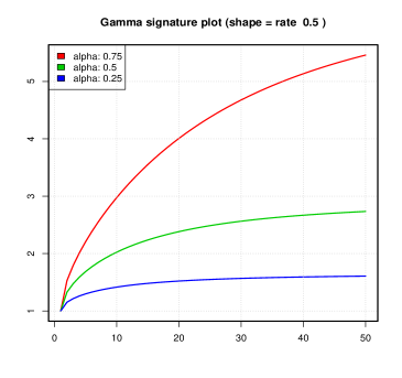
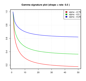
Figure 5: $\tau$ $\rightarrow$ $\bar{V}(\tau)$ when varying price return autocorrelation $\alpha$. Left: $\alpha$ $>$ $0$. Right: $\alpha$ $<$ $0$

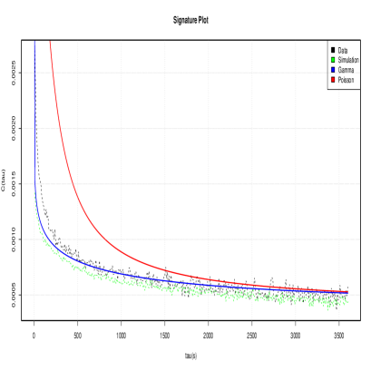
Figure 6: Comparison of signature plot: empirical data, simulated and computed

5 Conclusion and extensions

In this paper we used a Markov renewal process $(T_{n},J_{n})_{n}$ to describe the tick-by-tick evolution of the stock price and reproduce two important stylized facts, as the diffusive behavior and the decreasing shape of the mean signature plot towards the diffusive variance. Having in mind a direct application purpose, we decided to sacrifice the autocorrelation of inter-arrival times in order to have a fast and simple non-parametric estimation, perfect simulation and the suitable setup for a market making application, presented in a companion paper [10]. Aware of the model limits, and with an eye to statistical arbitrage, the next step is to extend the structure of the counting process $N_{t}$, for example to Hawkes process, to have a better fit, and the structure of the Markov chain $(J_{n})_{n}$ to a longer memory binary processes, able to recognize patterns. Another direction of study will be the extension to the multivariate asset price case.

Appendix A Appendix: Mean signature plot

The price process $P_{t}$ is given by

$$P_{t} = P_{0}+\sum_{k=1}^{N_{t}}J_{k}\;=\;\sum_{n=0}^{\infty}L_{n}1_{N_{t}=n},$$ (A.1)

where

$$L_{n} = \sum_{k=1}^{n}J_{k},\;\;\;n\geq 1,\;\;L_{0}\;=\;0.$$

Lemma A.1

Under (H), we have

$$\mathbb{E}_{\pi}\big{[}L_{n}^{2}\big{]} = n\frac{\sigma_{{}_{\infty}}^{2}}{\bar{\lambda}}-\frac{2\alpha}{1-\alpha}\frac{1-\alpha^{n}}{1-\alpha}\big{(}\mathbb{E}[\xi_{n}]\big{)}^{2},$$

where $\sigma_{{}_{\infty}}$ is defined in (3.1).

Proof. By writing that $L_{n}$ $=$ $L_{n-1}$ $+$ $\xi_{n}\hat{J}_{n}$, we have for $n$ $\geq$ $1$

$$\mathbb{E}_{\pi}\big{[}L_{n}^{2}\big{]} = \mathbb{E}_{\pi}\big{[}L_{n-1}^{2}+\xi_{n}^{2}\hat{J}_{n}^{2}+2\xi_{n}L_{n-1}\hat{J}_{n}\big{]}$$ (A.2)

$$= \mathbb{E}_{\pi}\big{[}L_{n-1}^{2}\big{]}+\mathbb{E}_{\pi}\big{[}\xi_{n}^{2}\big{]}+2\big{(}\mathbb{E}\big{[}\xi_{n}\big{]}\big{)}^{2}\sum_{k=1}^{n-1}\mathbb{E}_{\pi}\big{[}\hat{J}_{k}\hat{J}_{n}\big{]},$$

$$= \mathbb{E}_{\pi}\big{[}L_{n-1}^{2}\big{]}+\mathbb{E}_{\pi}\big{[}\xi_{n}^{2}\big{]}+2\big{(}\mathbb{E}\big{[}\xi_{n}\big{]}\big{)}^{2}\sum_{k=1}^{n-1}\mathbb{E}_{\pi}\big{[}\hat{J}_{k}\hat{J}_{0}\big{]}$$

where we used the fact that $\hat{J}_{n}^{2}$ $=$ $1$, $(\xi_{n})_{n}$ are i.i.d, and independent of $(\hat{J}_{n})_{n}$ in the second equality, and the stationarity of $(\hat{J}_{n})_{n}$ in the third equality. Now, from the Markov property of $(\hat{J}_{k})_{k}$ with probability transition matrix $\hat{Q}$ in (2.5) and (2.10), we have for any $k$ $\geq$ $1$:

$$\mathbb{E}_{\pi}\big{[}\hat{J}_{k}\hat{J}_{0}\big{]} = \mathbb{E}_{\pi}\Big{[}\mathbb{E}_{\pi}\big{[}\hat{J}_{k}|\hat{J}_{k-1}\big{]}\hat{J}_{0}\Big{]}$$

$$= \mathbb{E}\Big{[}\Big{(}\frac{1+\alpha}{2}\Big{)}\hat{J}_{k-1}\hat{J}_{0}-\Big{(}\frac{1-\alpha}{2}\Big{)}\hat{J}_{k-1}\hat{J}_{0}\Big{]}$$

$$= \alpha\mathbb{E}_{\pi}\big{[}\hat{J}_{k-1}\hat{J}_{0}\big{]},$$

from which we obtain by induction:

$$\mathbb{E}_{\pi}\big{[}\hat{J}_{k}\hat{J}_{0}\big{]} = \alpha^{k}.$$

Plugging into (A.2), this gives

$$\mathbb{E}_{\pi}\big{[}L_{n}^{2}\big{]} = \mathbb{E}_{\pi}\big{[}L_{n-1}^{2}\big{]}+\mathbb{E}_{\pi}\big{[}\xi_{n}^{2}\big{]}+\frac{2\alpha}{1-\alpha}(1-\alpha^{n-1})\big{(}\mathbb{E}[\xi_{n}]\big{)}^{2}.$$

By induction, we get the required relation for $\mathbb{E}_{\pi}\big{[}L_{n}^{2}\big{]}$. $\Box$

Consequently, we obtain the following expression of the mean signature plot:

Proposition A.1

Under (H), we have

$$\bar{V}(\tau) = \sigma_{{}_{\infty}}^{2}-\frac{2\alpha}{1-\alpha}\frac{1-G_{\alpha}(\tau)}{(1-\alpha)\tau}\big{(}\mathbb{E}[\xi_{n}]\big{)}^{2},\;\;\;\tau>0,$$ (A.3)

where $G_{\alpha}(t)$ $:=$ $\mathbb{E}_{\pi}[\alpha^{N_{t}}]$ $=$ $\sum_{n=0}^{\infty}\alpha^{n}\mathbb{P}_{\pi}[N_{t}=n]$.

Proof. From (4.2) and (A.1), we see that the mean signature plot is written as

$$\bar{V}(\tau) = \frac{1}{\tau}\sum_{n=0}^{\infty}\mathbb{E}_{\pi}[L_{n}^{2}]\mathbb{P}_{\pi}[N_{\tau}=n],$$

since the renewal process $N$ is independent of the marks $(J_{n})$. Together with the expression of $\mathbb{E}_{\pi}[L_{n}^{2}]$ in Lemma A.1, this yields

$$\bar{V}(\tau) = \frac{\sigma_{{}_{\infty}}^{2}}{\bar{\lambda}}\frac{\mathbb{E}_{\pi}[N_{\tau}]}{\tau}-\frac{2\alpha}{1-\alpha}\frac{1-G_{\alpha}(\tau)}{(1-\alpha)\tau}\big{(}\mathbb{E}[\xi_{n}]\big{)}^{2}.$$

Finally, since $\mathbb{E}_{\pi}[N_{\tau}]$ $=$ $\bar{\lambda}\tau$ by stationarity of $N$, we get the required relation. $\Box$

We now focus on the finite variation function $G_{\alpha}$ that we shall compute through its Laplace-Stieltjes transform:

$$\widehat{G}_{\alpha}(s) := \int_{0^{-}}^{\infty}e^{-st}dG_{\alpha}(t),\;\;\;s\geq 0.$$

We recall the convolution property for Laplace-Stieltjes transform

$$\widehat{G*H} = \widehat{G}.\widehat{H},$$

where

$$G*H(t) = \int_{0}^{t}G(t-s)dH(s).$$

Let us consider the function $Q_{\alpha}$ defined by:

$$Q_{\alpha}(t) := \sum_{n=0}^{\infty}\alpha^{n}\mathbb{P}_{\pi}[N_{t}\geq n].$$ (A.4)

Lemma A.2

Under (H), we have for all $\alpha$ $\neq$ $0$,

$$G_{\alpha} = \Big{(}1-\frac{1}{\alpha}\Big{)}Q_{\alpha}+\frac{1}{\alpha}$$ (A.5)

$$\widehat{Q}_{\alpha}(s) = 1+\alpha\frac{\bar{\lambda}}{s}\Big{(}\frac{1-\widehat{F}(s)}{1-\alpha\widehat{F}(s)}\Big{)}.$$ (A.6)

Proof. 1. For any $\alpha$ $\neq$ $0$, $t$ $\geq$ $0$, we have

$$G_{\alpha}(t) = \sum_{n=0}^{\infty}\alpha^{n}\mathbb{P}_{\pi}[N_{t}=n]\;=\;\sum_{n=0}^{\infty}\alpha^{n}\big{(}\mathbb{P}_{\pi}[N_{t}\geq n]-\mathbb{P}_{\pi}[N_{t}\geq n+1]\Big{)}$$

$$= \sum_{n=0}^{\infty}\alpha^{n}\mathbb{P}_{\pi}[N_{t}\geq n]-\frac{1}{\alpha}\Big{(}\sum_{n=0}^{\infty}\alpha^{n}\mathbb{P}_{\pi}[N_{t}\geq n]-\mathbb{P}_{\pi}[N_{t}\geq 0]\Big{)}$$

$$= Q_{\alpha}(t)-\frac{1}{\alpha}\Big{(}Q_{\alpha}(t)-1\Big{)},$$

which proves (A.5).

2. Recall that for the delayed renewal process $N$, the first arrival time $S_{1}$ is distributed according to the distribution $\Delta$ with density $\bar{\lambda}(1-F)$. Let us denote by $N^{0}$ the no-delayed renewal process, i.e. with all interarrival times $S_{n}^{0}$ $=$ $T_{n}^{0}-T_{n-1}^{0}$ distributed according to $F$, and by $Q_{\alpha}^{0}$ the function defined similarly as in (A.4) with $N$ replaced by $N^{0}$. Then,

$$Q_{\alpha}(t) = 1+\alpha\sum_{n=0}^{\infty}\alpha^{n}\mathbb{P}_{\pi}\big{[}N_{t}\geq n+1\big{]}$$ (A.7)

$$= 1+\alpha\sum_{n=0}^{\infty}\alpha^{n}\mathbb{P}_{\pi}[S_{1}+T_{n}^{0}\leq t]$$

$$= 1+\alpha\mathbb{E}_{\pi}\Big{[}\sum_{n=0}^{\infty}\alpha^{n}\mathbb{P}_{\pi}[T_{n}^{0}\leq t-S_{1}|S_{1}\leq t]\Big{]}$$

$$= 1+\alpha\mathbb{E}_{\pi}\Big{[}Q_{\alpha}^{0}(t-S_{1})1_{S_{1}\leq t}\Big{]}$$

$$= 1+\alpha Q_{\alpha}^{0}*\Delta(t),$$

By taking the Laplace-Stieltjes transform in the above relation, and from the convolution property, we get

$$\widehat{Q}_{\alpha} = 1+\alpha\widehat{Q_{\alpha}^{0}}\widehat{\Delta}.$$ (A.8)

By same arguments as in (A.7) and (A.8), we get $\widehat{Q_{\alpha}^{0}}$ $=$ $1+\alpha\widehat{Q_{\alpha}^{0}}\widehat{F}$, and so

$$\widehat{Q_{\alpha}^{0}} = \frac{1}{1-\alpha\widehat{F}}.$$ (A.9)

Now, from the relation $\Delta(t)$ $=$ $\int_{0}^{t}\bar{\lambda}(1-F(u))du$, and by taking Laplace-Stieltjes transform we get:

$$\widehat{\Delta}(s) = \frac{\bar{\lambda}}{s}\big{(}1-\widehat{F}(s)\big{)}.$$ (A.10)

By substituting (A.9) and (A.10) into (A.8), we get the required relation (A.6). $\Box$

From the relations (A.5)-(A.6) in the above Lemma, we immediately obtain the expression (4.3) for the Laplace-Stieltjes transform $\widehat{G}_{\alpha}$. Let us now derive the alternative integral expression (4.4) for $G_{\alpha}$.

Lemma A.3

Under (H), we have for all $\alpha$ $\neq$ $0$:

$$Q_{\alpha}(t) = 1+\bar{\lambda}t-\bar{\lambda}(1-\alpha)\int_{0}^{t}Q_{\alpha}^{0}(u)du,$$ (A.11)

with

$$Q_{\alpha}^{0}(t) = \displaystyle\sum_{n=0}^{\infty}\alpha^{n}F^{*(n)}(t),$$

and $F^{*(n)}$ is the $n$-fold convolution of the distribution function $F$.

Proof. We rewrite the expression (A.6) Laplace-Stieltjes transform as

$$\widehat{Q}_{\alpha}(s) = 1+\frac{\alpha\bar{\lambda}}{s}(1-\widehat{F})\sum_{n=0}^{\infty}(\alpha\widehat{F})^{n}$$ (A.12)

$$= 1+\frac{\alpha\bar{\lambda}}{s}\sum_{n=0}^{\infty}\alpha^{n}\Big{(}(\widehat{F})^{n}-(\widehat{F})^{n+1}\Big{)}.$$

Let us now consider the function $G_{\alpha}^{0}$ (resp. $Q_{\alpha}^{0}$) defined similarly as for $G_{\alpha}$ (resp. $Q_{\alpha}$) with $N$ replaced by $N^{0}$, the no-delayed renewal process with all interarrival times $S_{n}^{0}$ $=$ $T_{n}^{0}-T_{n-1}^{0}$ distributed according to $F$. Then,

$$G_{\alpha}^{0}(t) = \sum_{n=0}^{\infty}\alpha^{n}\big{(}\mathbb{P}_{\pi}[N_{t}^{0}\geq n]-\mathbb{P}_{\pi}[N_{t}^{0}\geq n+1]\Big{)}$$

$$= \sum_{n=0}^{\infty}\alpha^{n}\Big{(}\mathbb{P}_{\pi}[T_{n}^{0}\leq t]-\mathbb{P}_{\pi}[T_{n+1}^{0}\leq t]\Big{)}$$

$$= \sum_{n=0}^{\infty}\alpha^{n}\Big{(}F^{*(n)}-\ F^{*(n+1)})(t).$$

Therefore, the Laplace-Stieltjes transform of $G_{\alpha}^{0}$ is written also as

$$\widehat{G_{\alpha}^{0}} = \sum_{n=0}^{\infty}\alpha^{n}\Big{(}(\widehat{F})^{n}-(\widehat{F})^{n+1}\Big{)}.$$

By defining the function $I_{\alpha}^{0}(t)$ $:=$ $\int_{0}^{t}G_{\alpha}^{0}(u)du$, we then see from (A.12) that

$$\widehat{Q}_{\alpha}(s) = 1+\alpha\bar{\lambda}\widehat{I_{\alpha}^{0}},$$

and thus

$$Q_{\alpha}(t) = 1+\alpha\bar{\lambda}\int_{0}^{t}G_{\alpha}^{0}(u)du.$$ (A.13)

Finally, by same arguments as in (A.5), we have

$$G_{\alpha}^{0} = \Big{(}1-\frac{1}{\alpha}\Big{)}Q_{\alpha}^{0}+\frac{1}{\alpha},$$

and plugging into (A.13), we get the required result. $\Box$

By using (A.5) and (A.11), we then obtain the integral expression (4.4) of the function $G_{\alpha}$ as in Proposition 4.1. Finally, we derive the asymptotic behavior of the mean signature plot.

Proposition A.2

Under (H), we get:

$$\bar{V}(\infty)\;:=\;\lim_{\tau\rightarrow\infty}\bar{V}(\tau) = \sigma^{2}_{{}_{\infty}},$$ (A.14)

$$\bar{V}(0^{+})\;:=\;\lim_{\tau\downarrow 0^{+}}\bar{V}(\tau) = \bar{\lambda}\mathbb{E}[\xi_{n}^{2}],$$ (A.15)

and

$$\bar{V}(0^{+})>\bar{V}(\infty) \alpha<0.$$ if and only if

Proof. By observing that the function $G_{\alpha}$ is stricly bounded in $\tau$ by $1$ for any $\alpha$ $\in[-1,1)$, we easily obtain from the expression (A.3) the limit for $\bar{V}(\tau)$ when $\tau$ goes to infinity.

On the other hand, by substituting the integral formula (4.4) of the function $G_{\alpha}$ into the expression (A.3) of the mean signature plot, we have:

$$\bar{V}(\tau) = \sigma_{{}_{\infty}}^{2}-\frac{2\alpha}{1-\alpha}\big{(}\mathbb{E}[\xi_{n}]\big{)}^{2}\Big{(}\frac{\bar{\lambda}}{\alpha}\Big{)}\Big{(}1-\big{(}1-\alpha\big{)}\frac{1}{\tau}\int_{0}^{\tau}Q_{\alpha}^{0}(s)ds\Big{)}$$

Next, by noting that

$$\lim_{\tau\rightarrow 0^{+}}\frac{1}{\tau}\int_{0}^{t}Q_{\alpha}^{0}(s)ds = Q_{\alpha}^{0}(0)\;=\;1,$$

we deduce that

$$\lim_{\tau\rightarrow 0^{+}}\bar{V}(\tau) = \sigma_{{}_{\infty}}^{2}-\frac{2\bar{\lambda}\alpha}{1-\alpha}\big{(}\mathbb{E}[\xi_{n}]\big{)}^{2},$$ (A.16)

which gives (A.15) from the expression (3.1) of $\sigma_{{}_{\infty}}^{2}$. Finally, we immediately see from (A.16) that $\bar{V}(0^{+})>\bar{V}(\infty)$ if and only if $\alpha$ $<$ $0$. $\Box$

References

- [1] Abergel F. and W. Jedidi (2011): “A mathematical approach to order book modeling”, to appear in International Journal of Theoretical and Applied Finance.
- [2] Ait-Sahalia Y., Mykland P. and L. Zhang (2011): “Ultra high frequency volatility estimation with dependent microstructure noise”, Journal of Econometrics, vol. 160, 160-175.
- [3] Bacry E., Delattre S., Hoffman M. and J.F. Muzy (2013): “Modeling microstructure noise with mutually exciting point processes”, Quantitative Finance, vol 13, 65-77.
- [4] Bauwens L. and N. Hautsch (2009): Modeling financial high frequency data using point processes, Handbook of Financial time series, Springer Verlag.
- [5] Bouchaud J.P. and M. Potters (2004): Theory of financial risk and derivative pricing, from statistical physics to risk management, Cambridge university press, 2nd edition.
- [6] Cont R. and A. de Larrard (2010): “Price Dynamics in a Markovian Limit Order Market”, to appear in SIAM Journal of Financial Mathematics.
- [7] Dacorogna M., Gencay R., Muller U.A., Olsen R. and O.V. Pictet (2001): An introduction to high frequency finance, Academic press, 383.
- [8] Daley D. and D. Vere-Jones (2002): An introduction to the theory of point processes, vol 1, 2nd edition, Springer.
- [9] Fauth A. and C. Tudor (2012): “Modeling first line of an order book with multivariate marked point processes”, preprint.
- [10] Fodra P. and H. Pham (2013): “High frequency trading in a Markov renewal model”.
- [11] Glynn P. and P. Haas (2004): “On functional central limit theorems for semi-Marlov and related processes”, Communications in Statistics, Theory and Methods, 33 (3), 487-506.
- [12] Gloter A. and J. Jacod (2001): “Diffusion with measurement errors I and II”, ESAIM Prob. and Stats, 5, 225-242 and 243-260.
- [13] Limnios N. and G. Oprisan (2001): Semi-Markov processes and reliability, Birkhauser.
- [14] Rosenbaum M. and and C. Y. Robert (2011): ”A new approach for the dynamics of ultra high frequency data: the model with uncertainty zones”, Journal of Financial Econometrics, 9(2), 344-366.