The Galactic Center: Not an Active Galactic Nucleus

Abstract

We present $10\ \mu$m–$35\ \mu$m Spitzer spectra of the interstellar medium in the Central Molecular Zone (CMZ), the central $210$ pc $\times$ $60$ pc of the Galactic center (GC). We present maps of the CMZ in ionic and H₂ emission, covering a more extensive area than earlier spectroscopic surveys in this region. The radial velocities and intensities of ionic lines and H₂ suggest that most of the H₂ 0–0 S(0) emission comes from gas along the line-of-sight, as found by previous work. We compare diagnostic line ratios measured in the Spitzer Infrared Nearby Galaxies Survey (SINGS) to our data. Previous work shows that forbidden line ratios can distinguish star-forming galaxies from LINERs and AGNs. Our GC line ratios agree with star-forming galaxies and not with LINERs or AGNs.

1. Introduction

The Galactic center (GC) is the closest galactic nucleus. At a distance of $7.9\pm 0.8$ kpc (Reid et al., 2009), $1$ pc in the GC corresponds to only $26\arcsec$. The GC provides an opportunity to unveil interactions between various physical processes in a nuclear environment of a galaxy with excellent spatial resolution unapproachable for other galaxies.

The central $170\arcmin\times 40\arcmin$ ($\sim 400$ pc $\times 90$ pc) region of the Galaxy is often called the Central Molecular Zone (CMZ; Morris & Serabyn, 1996). The CMZ is a massive molecular cloud complex in the Galaxy, which contains about 10% of the Galaxy’s molecular gas and produces 5%–10% of its infrared (IR) and Lyman continuum luminosity (Smith et al., 1978; Nishimura et al., 1980; Bally et al., 1987, 1988; Morris & Serabyn, 1996). Earlier radio continuum surveys revealed that the CMZ is an active star forming region and contains the most active star forming cloud in the entire Galaxy, the Sagittarius B2 (Sgr B2) complex. Herschel observations revealed that the dust emission from the CMZ mainly arises in a ring-like structure (Molinari et al., 2011). In this paper, we use the terms CMZ and GC interchangeably, referring to the same $\sim 200$ pc region in the center of the Galaxy.

Star formation in the CMZ is inevitably affected by the extreme physical conditions of the natal clouds, which have an order of magnitude higher gas density than in the disk, with high gas temperature, pressure, turbulence, strong tidal shear, and milli-Gauss magnetic field strengths (Morris & Serabyn, 1996). Because of these unusual conditions not found in nearby normal star-forming regions in the disk, the nature of star formation in the CMZ is a subject of active research.

A key to unlocking the secrets of star formation activities in the CMZ is a detailed spectroscopic study of its interstellar medium (ISM) over a wide range of wavelengths. Mid-IR emission lines are particularly useful in analyzing the physical properties of the GC gas because it lies behind heavy dust obscuration ($A_{V}\sim 30$ mag). Forbidden emission lines in the mid-IR are generally insensitive to electron gas temperatures, and can be used to determine physical properties such as the electron density and ionization parameters, and to identify sources of ionization. Furthermore, molecular hydrogen emission from pure rotational transitions can be observed in the mid-IR, which may hold vital clues to gas heating mechanisms in the CMZ.

A mid-IR spectroscopic survey of the GC was previously conducted at $2\ \mu$m–$196\ \mu$m based on ISO observations (Rodríguez-Fernández et al., 2001a, 2004; Rodríguez-Fernández & Martín-Pintado, 2005). They observed $15$ different lines of sight to molecular clouds in the CMZ (see Figure 1 in Rodríguez-Fernández & Martín-Pintado, 2005). Rodríguez-Fernández et al. (2001a, 2004) used observations of molecular hydrogen emission to discuss heating mechanisms of warm molecular gas in the CMZ, and concluded that low-density photon dominated regions (PDRs) and low-velocity shocks ($v<10$ km s^-1) are required to explain the temperatures derived from the warm molecular gas. Rodríguez-Fernández & Martín-Pintado (2005) analyzed fine structure lines in the GC far from thermal continuum sources and massive clusters. They concluded that the ionizing radiation field is rather constant throughout the CMZ, suggesting ionization by relatively hot and distant stars, and found that excitation ratios, temperatures, and ionization parameters of ionized gas in the CMZ are similar to those found in some low-excitation starburst galaxies.

A more recent survey in the mid-IR was carried out by Simpson et al. (2007) using the Infrared Spectrograph (IRS; Houck et al., 2004) onboard the Spitzer Space Telescope (Werner et al., 2004), which has a higher sensitivity than ISO at $10\ \mu$m–$38\ \mu$m. The Simpson et al. survey consists of high-resolution spectra of $38$ positions along a narrow $24\arcmin$ long strip at a Galactic longitude $l\approx+0.1\arcdeg$. Simpson et al. measured several forbidden emission lines and molecular hydrogen lines to constrain the physical conditions of clouds near the Quintuplet Cluster, the Arches Cluster, the Radio Arc Bubble (Rodríguez-Fernández et al., 2001), and Arched Filaments. They concluded from their observations that the main source of excitation in the GC is photo-ionization from the massive star clusters and that multi-component PDR models can explain the observed line emission from molecular hydrogen (see also Contini, 2009). Simpson et al. also concluded that shocks in the Radio Arc Bubble are responsible for strong [O IV] emission.

In our recent spectroscopic survey of massive young stellar objects (YSOs) in the CMZ (An et al., 2009, 2011), we used Spitzer/IRS to collect an extensive set of mid-IR spectra for $107$ YSO candidates. The goal of this survey was to discover and characterize the spectroscopic properties of massive YSOs in the GC. To achieve this original goal, we spent half of our observing time on background spectra near each YSO candidate because of the strong and spatially variable background emission in the GC. Our GC background spectra, which are the by-product of our YSO observing program, now constitute the largest and most comprehensive mid-IR spectroscopic data set available to study the properties of the ionized and molecular gas in the star-forming nucleus of the Galaxy.

In this paper, we present panoramic mapping results from ionic and molecular hydrogen emission lines throughout the entire CMZ. Data acquisition and spectral analysis are presented in § 2. Line intensities and radial velocities in the CMZ are presented in § 3. Mid-IR line ratio diagnostics are used to compare the physical properties of the Galactic nucleus to those of other nearby galaxies in § 4. Our results are summarized in § 5.

2. Method

2.1. Observations and Extraction of Spectra

The IRS spectra presented in this paper were obtained in May and October 2008 as part of Spitzer Cycle 4, during our observing program to identify massive YSOs in the GC (Program ID: 40230, PI: S. Ramírez). We targeted $107$ point sources with extremely red colors on near- and mid-IR color-color diagrams as YSO candidates (see An et al., 2011, for details). The positions of our spectra are shown in the top panel of Figure 1, on top of the Spitzer/IRAC $8\ \mu$m image (Stolovy et al., 2006; Ramírez et al., 2008). Our survey encompasses a large area in the flattened CMZ cloud complex ($|b|\lesssim 0.24\arcdeg$), covering regions near strong radio continuum sources (Sgr A, Sgr B1, Sgr B2, and Sgr C), massive star clusters (the Quintuplet, Arches, and Central clusters), and the Radio Bubble (see the bottom panel of Figure 1).

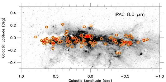
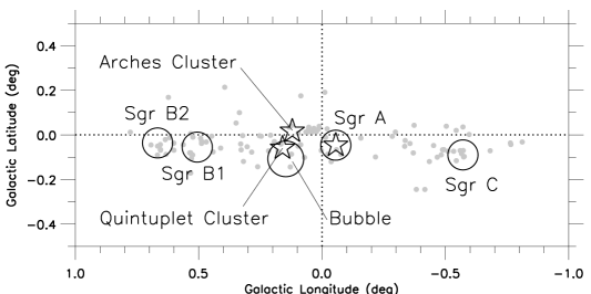
Figure 1.— Top: Spatial distribution of 107 Spitzer/IRS targets on the IRAC $8.0\ \mu$m image (Stolovy et al., 2006; Ramírez et al., 2008) of the Galactic center (GC). The above image shows the entire Central Molecular Zone (CMZ), which covers approximately $170\arcmin\times 40\arcmin$ ($\sim 400$ pc $\times 90$ pc) centered on the GC. Our IRS point-source targets (An et al., 2009, 2011) are marked with $1\arcmin$ ($2.3$ pc) radius circles. In this paper, we analyze the GC interstellar medium (ISM) as measured by four background spectra that are $\sim 1\arcmin$ away from each target. Bottom: Schematic diagram of locations of the CMZ molecular complexes (Sgr A, Sgr B1, Sgr B2, and Sgr C; large open circles), the Radio Bubble (large open circle), and star clusters (Quintuplet, Arches, and Central clusters; open star symbols). The grey circles represent the location of the Spitzer/IRS targets.

In our Spitzer program, massive YSO candidates were observed using both high- and low-resolution IRS modules. In this work, however, we utilize only the high-resolution observations taken with the short-high (SH; $9.9\ \mu$m$-19.6\ \mu$m, $\lambda/\Delta\lambda\sim 600$; $4.7\arcsec\times 11.3\arcsec$ or $0.18$ pc $\times 0.43$ pc slit entrance) and the long-high (LH; $18.7\ \mu$m$-37.2\ \mu$m, $\lambda/\Delta\lambda\sim 600$; $11.1\arcsec\times 22.3\arcsec$ or $0.43$ pc $\times 0.85$ pc slit entrance) modules. These two modules share the same slit centers on the sky.

Four background spectra were taken at $\sim 1\arcmin$ ($2.3$ pc) away from each of the YSO candidates; the positions of these points can be glimpsed by looking at the open circles in the top panel of Figure 1, each of which has a $1\arcmin$ radius. The exact locations of these spectra were carefully chosen by visual inspection to avoid bright point sources on the IRAC $8\ \mu$m image (Stolovy et al., 2006; Ramírez et al., 2008), and were intended to provide a level of background mid-IR emission similar to that of the target position. As shown in Figure 1, our background spectra are somewhat uniformly distributed over a $\sim 90\arcmin\times 25\arcmin$ ($\sim 210$ pc $\times 60$ pc) region in the CMZ.

We reduced IRS spectra from the basic calibrated data (BCD) products version S18.7.0. We corrected for rogue pixel values using the software package IRSCLEAN provided by Spitzer Science Center (SSC), and applied the DARKSETTLE software package to the LH frames to correct for non-uniform dark current. We extracted SH and LH spectra using the SPICE tool in an “extended” extraction mode (with slit loss corrections for a source infinite in extent), and further corrected for fringe patterns using the IRSFRINGE package. More information on our IRS observations and basic data reduction is found in An et al. (2011).

The contribution of zodiacal light is relatively high in the GC, typically amounting to $\sim 10\%$–$30\%$ of the continuum emission from the ISM in the IRS spectral range. We used the zodiacal light estimator in the SSC-provided software SPOT, which is based on COBE/DIRBE measurements, to determine the contribution from the zodiacal light in each season. The zodiacal spectrum has a peak emission of $\sim 40\ {\rm MJy\ sr^{-1}}$ at $20\ \mu$m, with a $\sim 10\%$ seasonal variation. We constructed a smoothed zodiacal spectrum using quadratic interpolation, and then subtracted it from the extracted spectra. Since our IRS targets are found within a degree of the GC, spatial variations in the zodiacal emission are negligible. The correction for zodiacal emission has no direct impact on emission line flux measurements, but has an influence on the extinction correction since we measure foreground extinction from the continuum emission near the $10\ \mu$m silicate feature (see § 2.3).

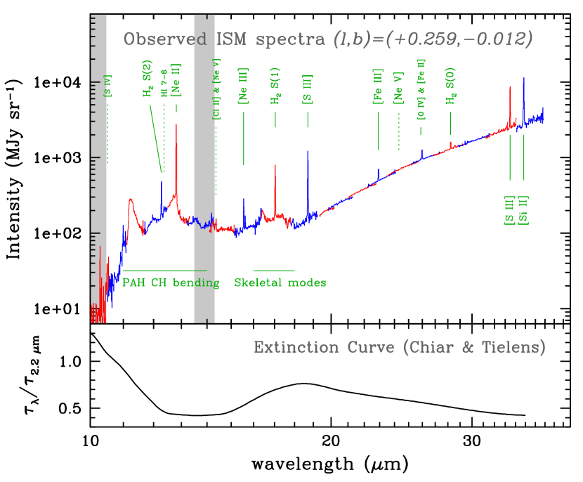
Figure 2.— Top: Observed Spitzer/IRS spectrum in the ISM of the GC, measured at $(l,b)=(+0.2588\arcdeg,-0.0119\arcdeg)$, after subtracting the zodiacal emission. Different spectral orders are shown in alternating colors. Ionic forbidden emission lines and molecular hydrogen lines are marked with vertical lines, with dotted lines indicating non-detected emission lines. Vertical grey strips centered at $10.2\ \mu$m and $13.9\ \mu$m mark continuum regions used to estimate the $9.7\ \mu$m silicate optical depth ($\tau_{9.7}$) for each line of sight (see text). Bottom: Extinction curve for the GC, normalized to the extinction value in the $K$ passband (Chiar & Tielens, 2006).

We used the above procedure to obtain ISM spectra from SH and LH for $428$ individual lines of sight in the GC (i.e., four background spectra for each of $107$ point-source targets). Figure 2 shows one of the observed spectra in the GC, after the zodiacal light correction. Different IRS spectral orders are shown in alternating colors. Forbidden emission lines and molecular hydrogen lines are marked, and the wavelength ranges of strong polycyclic aromatic hydrocarbon (PAH) emission features are indicated.

We identified spectral orders that best display individual lines, and used Gaussian profile fits to compute line fluxes, as described in the following section. Figure 2 shows that order tilts are present in some of the IRS spectra. In An et al. (2011), we used low-resolution spectra to correct for order tilts before we combined individual high-resolution spectra from different orders. In the following analysis, however, we combined spectra without order-tilt corrections, because our low-resolution background slits are not always co-spatial with the high-resolution slit positions. Figure 2 shows that the line fluxes should not be strongly affected by the order tilts.

2.2. Measurement of Emission Line Strengths and Radial Velocities

We measured emission line fluxes from several ionic fine-structure lines, as well as molecular hydrogen lines from pure rotational transitions, H₂ 0–0 S(0), H₂ 0–0 S(1), and H₂ 0–0 S(2). A list of emission lines included in this paper is shown in Table 1, in order of increasing wavelength. In addition to these lines, we attempted to measure a flux from other ionic features such as [Ar V] $13.1\ \mu$m, [P III] $17.89\ \mu$m, [Fe II] $17.94\ \mu$m, [Fe II] $24.52\ \mu$m, and [Fe II] $35.35\ \mu$m, but none of these features were strong enough to be detected. The third column in Table 1 shows IRS modules and spectral orders, from which individual line fluxes were measured (see below). The fourth column shows normalized extinction coefficients from the GC extinction curve in Chiar & Tielens (2006); see also the bottom panel of Figure 2. The ionization potential for each ion is listed in the last column in Table 1.

Table 1Emission Lines Detected in Spitzer/IRS Spectra

Line	Wavelength	IRS Module/Order	$A_{\lambda}$/$A_{K}$	IP
	($\mu$m)			(eV)
[S IV]	$10.51$	SH/19	$1.080$	$34.79$
H2 S(2)	$12.28$	SH/17	$0.478$	$\cdots$
H I 7-6	$12.37$	SH/17	$0.462$	$\cdots$
[Ne II]	$12.81$	SH/16	$0.435$	$21.56$
[Ne V]	$14.32$	SH/14	$0.430$	$97.12$
[Cl II]	$14.37$	SH/14	$0.431$	$12.97$
[Ne III]	$15.56$	SH/13	$0.533$	$40.96$
H2 S(1)	$17.04$	SH/12	$0.698$	$\cdots$
[S III]	$18.71$	SH/11	$0.762$	$23.34$
[Fe III]	$22.93$	LH/17	$0.622$	$16.19$
[Ne V]	$24.32$	LH/16	$0.595$	$97.12$
[O IV]	$25.89$	LH/15	$0.562$	$54.94$
[Fe II]	$25.99$	LH/15	$0.560$	$7.90$
H2 S(0)	$28.22$	LH/14	$0.513$	$\cdots$
[S III]	$33.48$	LH/12	$0.433$	$23.34$
[Si II]	$34.82$	LH/11	$0.426$	$8.15$

Figure 3 shows examples of the line profile fits for the emission lines listed in Table 1. Grey histograms are observed IRS spectra from various lines of sight. The red line represents the best-fitting Gaussian profile, obtained using the non-linear least squares fitting routine MPFIT (Markwardt, 2009). The underlying blue line shows a local continuum constructed from a 1^st–3^rd order polynomial fit to the continuum points on each side of the emission line. A standard deviation of data points from the continuum line was used as an effective $1\sigma$ error per data point in the profile fitting. High order polynomials were used to determine a local continuum near PAH emission features. Simultaneous fits of two Gaussian profiles were made for two sets of blended emission lines, [Ne V] $14.32\ \mu$m and [Cl II] $14.37\ \mu$m, and [O IV] $25.89\ \mu$m and [Fe II] $25.99\ \mu$m.

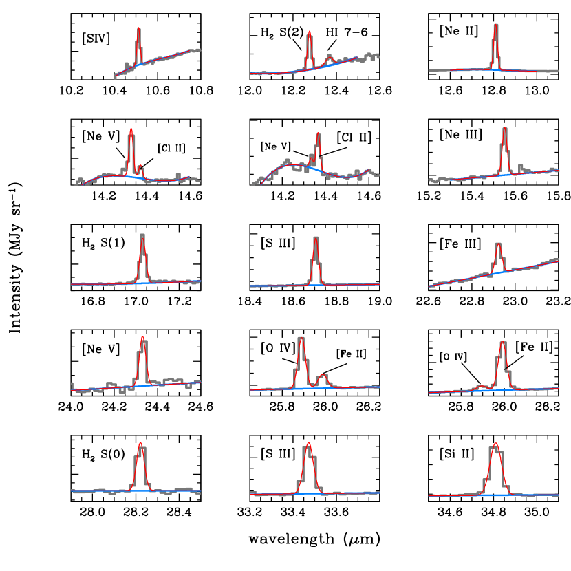
Figure 3.— Examples of line profile fits for the GC ISM spectra. Grey histograms show observed Spitzer/IRS spectra, displayed over the same wavelength interval, but with an arbitrary intensity scale on the vertical axis. Ionic emission lines as well as pure rotational lines from molecular hydrogen, such as H₂ $0-0$ S(0), H₂ $0-0$ S(1), and H₂ $0-0$ S(2), are shown. The best-fitting Gaussian profile is shown as a red line on top of a local continuum (blue line).

The total line flux was computed by integrating the underlying flux of the best fitting Gaussian profile in wavenumber space. Errors in these line fluxes were estimated by adding in quadrature the $1\sigma$ flux uncertainties derived from uncertainties in the height and width of the Gaussian fit, or by propagating $1\sigma$ errors in the local continuum, whichever is larger. The latter was computed as

$$\sigma_{\rm flux}\approx F_{\rm rms}\ \Delta\nu_{\rm max}\approx F_{\rm rms}\ \left(\frac{c}{\lambda^{2}}\right)\Delta\lambda_{\rm max},$$ (1)

where $F_{\rm rms}$ is the rms dispersion in the local continuum. The parameter $\Delta\lambda_{\rm max}$ is the maximum value of the full-width at half-maximum (FWHM) of the line profile set in the Gaussian line fitting, which we assumed to be $\Delta v=600$ km s^-1 for all lines. In most cases, errors propagated from Gaussian fits were larger than those estimated using Equation 1.

The line center was allowed to vary in our line fitting procedure, from which we measured line-of-sight velocities ($v_{r}$) from individual emission lines. Although high-resolution spectra from Spitzer/IRS have a relatively low spectral resolution ($R\equiv\Delta\lambda/\lambda=600$), radial velocities can be obtained with a precision of a few tens of kilometers per second for strong emission lines (e.g., Simpson et al., 2007). We computed radial velocities in the Local Standard of Rest (LSR), after correcting for the spacecraft motion: the correction terms (keyword VLSRCORR provided by the SSC) for May and October 2008 observing runs were $+38.9$ km/s and $-18.5$ km/s, respectively.

The accuracy of our radial velocity measurements was evaluated as follows. First of all, we compared $v_{r}$ measurements from the same ionic species, [S III] $18.71\ \mu$m and [S III] $33.48\ \mu$m, which are found on two different IRS modules. We found that the mean difference in $v_{r}$ between these lines is $\Delta v_{r}=31$ km s^-1, indicating the error from a module-to-module and/or order-to-order change in the IRS wavelength calibration. In addition, the scatter in the $v_{r}$ difference from these two lines is $\sigma_{v}=17$ km s^-1, which is a measure of the precision in the $v_{r}$ determination.

The size of systematic errors in $v_{r}$ can be further examined by comparing $v_{r}$ determined among strong ionic emission lines. We used [Ne II] $12.81\ \mu$m as a basis of comparison in $v_{r}$. We found a median difference in $v_{r}$ for all of the IRS spectra at $l\leq+0.2\arcdeg$ as follows: $\Delta v_{r}=+5.3$ km s^-1 for [Ne III] $15.56\ \mu$m, $\Delta v_{r}=-10.8$ km s^-1 for [S III] $18.71\ \mu$m, $\Delta v_{r}=+21.7$ km s^-1 for [S III] $33.48\ \mu$m, and $\Delta v_{r}=+71.1$ km s^-1 for [Si II] $34.82\ \mu$m, respectively, in the sense that a positive difference indicates a larger $v_{r}$ from a given line than from [Ne II]. We used these $\Delta v_{r}$ values to first shift all ionic lines to the [Ne II] velocity. The [Ne II] line has on average a smaller $v_{r}$ by $\Delta v_{r}=22.60$ km s^-1 than the mean $v_{\rm LSR}=+51.0$ km s^-1 measured from a hydrogen recombination line in Sgr B1 (Mehringer et al., 1992). We thus applied this second correction to shift all ionic lines to match Mehringer et al. (1992) in Sgr B1.

Molecular hydrogen lines from pure rotational transitions are also strong enough to be detected in the GC and provide radial velocities. We compared $v_{r}$ from individual IRS spectra to the peak $v_{r}$ of CO $J=4\rightarrow 3$ emission (Martin et al., 2004) at $-0.2\arcdeg<l<1.0\arcdeg$, and found $\Delta v_{r}=+62.5$ km s^-1, $+51.2$ km s^-1, and $+29.4$ km s^-1, for H₂ S(2) $12.28\ \mu$m, H₂ S(1) $17.04\ \mu$m, and H₂ S(0) $28.22\ \mu$m, respectively. The sense of the difference is that radial velocities from these lines are on average lower than those from the CO line. We then shift all H₂ lines to the CO velocity.

The above systematic offsets in the measured $v_{r}$ indicate that the wavelength calibration error in the Spitzer/IRS spectra is on the order of at least a few tens of kilometers per second. To summarize, we put all $v_{r}$ measurements from the IRS observations in the Local Standard of Rest (LSR) by applying zero-point offsets to $v_{r}$.

2.3. Foreground Extinction Estimates

We corrected line flux measurements for foreground extinction between the GC and the Sun. This was done on a spectrum-to-spectrum basis, because of the patchy dust extinction in the GC. We utilized two different approaches to correcting for foreground extinction.

The first approach is based on the method developed in Simpson et al. (2007), who determined the flux ratio at $10\ \mu$m and $14\ \mu$m ($F_{14}/F_{10}$) and used it to infer the optical depth of the $9.7\ \mu$m silicate absorption feature ($\tau_{9.7}$) near the Radio Arc Bubble. Following the Simpson et al. prescription, we estimated mean fluxes at $10.00\ \mu$m $\leq\lambda\leq 10.48\ \mu$m and $13.50\ \mu$m $\leq\lambda\leq 14.30\ \mu$m from SH spectra after a $3\sigma$ rejection. As shown by vertical grey strips in Figure 2, these two continuum wavelength ranges are almost free of PAHs features and ionic emission lines. Then we estimated $\tau_{9.7}$ for each line of sight, by using a simple linear relationship between the $9.7\ \mu$m silicate optical depth and the continuum flux ratio, $\tau_{9.7}=(\ln{(F_{14}/F_{10})}-0.809)/0.560$, which was inferred from tabulated values in Simpson et al. (2007). The top panel in Figure 4 shows the spatial distribution of $\tau_{9.7}$ derived in this way for all lines of sight in our program.

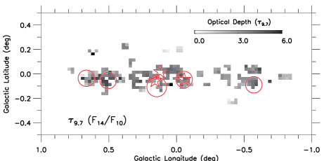
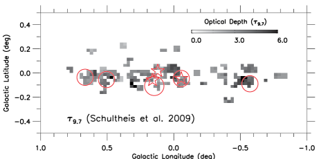
Figure 4.— Extinction maps shown as the silicate optical depth at $9.7\ \mu$m ($\tau_{9.7}$) in the line of sight to the GC. Each pixel covers $1.5\arcmin\times 1.5\arcmin$ ($\sim 3.5$ pc $\times 3.5$ pc), and key features of the GC are overlaid (see Figure 1). Top: The $9.7\ \mu$m silicate optical depth inferred from the ratio of $10\ \mu$m and $14\ \mu$m continuum fluxes based on the Simpson et al. (2007) method. Bottom: The $9.7\ \mu$m silicate optical depth from the Schultheis et al. (2009) extinction map, which is based on 2MASS and Spitzer/IRAC colors of GC giants. We convert $A_{V}$ from Schultheis et al. (2009) into $\tau_{9.7}$ by adopting $A_{V}/\tau_{9.7}=9$ (Roche & Aitken, 1985).

Alternatively, we utilized the $A_{V}$ extinction map toward the GC (Schultheis et al., 2009) based on the observed stellar locus of red giant stars on 2MASS and Spitzer/IRAC color-color diagrams. The bottom panel in Figure 4 shows the distribution of $\tau_{9.7}$ from Schultheis et al. (2009), after converting their $A_{V}$ values into $\tau_{9.7}$ using $A_{V}/\tau_{9.7}=9$ (Roche & Aitken, 1985).

Figure 5 compares $\tau_{9.7}$ derived using the Simpson et al. (2007) method to the visual extinction ($A_{V}$) from Schultheis et al. (2009). Figure 5 shows a large scatter between these two independent extinction estimates. However, their mean trend agrees well with the GC relation (Roche & Aitken, 1985, $A_{V}/\tau_{9.7}=9$). For comparison, we also show the relationship for the local ISM (Roche & Aitken, 1984, $A_{V}/\tau_{9.7}=18.5$) in Figure 5, which does not match the observed trend in the GC at all.

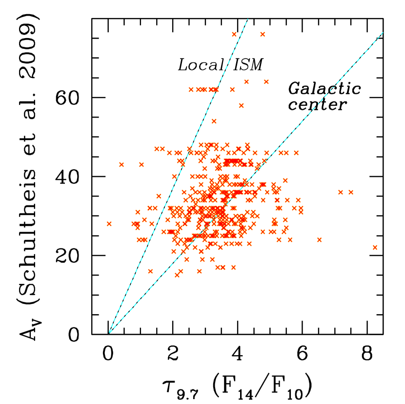
Figure 5.— Comparison between the silicate optical depth at $9.7\ \mu$m ($\tau_{9.7}$) derived using the Simpson et al. (2007) method (F₁₄/F₁₀) and the visual extinction ($A_{V}$) from the Schultheis et al. (2009) extinction map for all of the IRS background spectra. Dashed lines are previously measured relationships in the line of sight to the GC ($A_{V}/\tau_{9.7}=9$; Roche & Aitken, 1985) and for the local ISM ($A_{V}/\tau_{9.7}=18.5$; Roche & Aitken, 1984), respectively.

In the following analysis, we derived $\tau_{9.7}$ using Simpson et al. (2007) method and present results after correcting line fluxes for extinction, unless otherwise stated. However, we repeated our analysis with foreground extinction from the Schultheis et al. (2009) map, and compared results with each other. As shown below, our main results are solid, and are only weakly dependent on the specific choice of foreground extinction correction.

In addition to the above extinction corrections, we further corrected observed line fluxes from [Ne III] $15.56\ \mu$m for the absorption induced by CO₂ ice grains on a spectrum-to-spectrum basis. We used the same procedure as in An et al. (2011) to decompose a wide CO₂ ice absorption band over $\sim 15\ \mu$m–$16\ \mu$m using five laboratory spectral components of different CO₂ ice mixtures, and obtained an optical depth of the CO₂ ice from the best-fitting model profile. The mean optical depth from all of the GC ISM spectra is $\langle\Delta\tau\rangle=0.065$ at the position of the [Ne III] line. The relatively small optical depth at $15.56\ \mu$m is because the [Ne III] line is located in the long-wavelength wing of the CO₂ ice absorption, in addition to the fact that the CO₂ ice band in the ISM is weaker and narrower than those seen in massive YSOs (see An et al., 2011).

For a given $\tau_{9.7}$, we corrected a line flux for interstellar extinction at each wavelength using

$$A_{\lambda}=\left(\frac{A_{\lambda}}{A_{K}}\right)\left(\frac{A_{K}}{A_{V}}\right)\left(\frac{A_{V}}{\tau_{9.7}}\right)\tau_{9.7},$$ (2)

where $A_{\lambda}/A_{K}$ is the GC extinction curve value in Chiar & Tielens (2006), normalized to the extinction in the $K$ bandpass (see Table 1). We adopted $A_{K}/A_{V}\approx 0.11$ (Figer et al., 1999) and the GC relation of $A_{V}/\tau_{9.7}=9$ as determined by Roche & Aitken (1985). The extinction-corrected line flux was then obtained using

$$\log{f_{0}}=\log{f_{\rm obs}}+0.4A_{\lambda}.$$ (3)

2.4. Coadded GC ISM Spectra

In addition to individual ISM spectra, we also created and analyzed a coadded GC spectrum as shown in Figure 6. This allows us to compare the ISM spectrum measured across $\sim 200$ pc to the individual spectra with the $\sim 3.5$ pc resolution. We constructed the coadded IRS spectrum by summing fluxes from $428$ individual high-resolution spectra in the GC. The top panel in Figure 6 shows the spectrum coadded without any foreground extinction correction. The bottom panel displays the result of correcting each individual spectrum for extinction based on the Simpson et al. (2007) method (§ 2.3), then coadding the corrected spectra. We also illustrate the spectrum created by correcting each individual spectrum for extinction with the Schultheis et al. (2009) extinction map, then coadding. The coadded spectra from each extinction correction method are very similar. We present below line fluxes from the coadded spectrum together with those obtained from individual spectra.

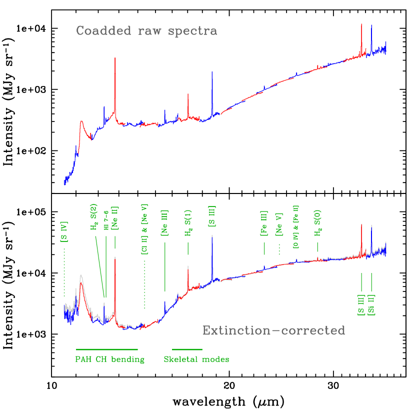
Figure 6.— Coadded GC ISM spectra constructed from 428 high-resolution IRS spectra. Locations of ionic forbidden emission lines and molecular hydrogen lines are marked, where dotted lines indicate positions of weakly detected emission lines. Top: Coadded spectrum created by adding fluxes from individual IRS spectra without foreground extinction corrections. Bottom: Same as in the top panel, but coadded after correcting individual spectra for extinction based on the Simpson et al. (2007) method. Underlying grey line shows the same but with extinction corrections based on the Schultheis et al. (2009) extinction map. Different spectral orders are shown in alternating colors.

3. Results

3.1. Panoramic Emission Line Mapping in the GC

Panoramic emission line maps are displayed in Figure 7 in a logarithmic flux scale for each line. Only those lines detected at more than a $3\sigma$ level were included. Table 2 provides the individual line fluxes used in these maps, after correcting for dust extinction using the Simpson et al. (2007) technique. Only a portion of Table 2 is shown here to demonstrate its form and content, and a machine-readable version of the full table is available in the electronic edition of the Journal.

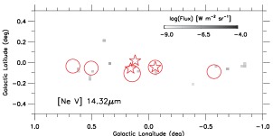
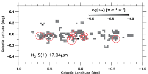
Figure 7.— Panoramic emission line maps in the GC. Line intensities from individual spectra are averaged together within each $1.5\arcmin\times 1.5\arcmin$ ($\sim 3.5$ pc $\times 3.5$ pc) pixel if the lines are detected at more than a $3\sigma$ level. Average line intensities are shown in a logarithmic scale (W m^-2 sr^-1), after correcting for foreground extinction ($\tau_{9.7}$) derived from the ratio between $10\ \mu$m and $14\ \mu$m continuum fluxes ($F_{14}/F_{10}$; see top panel in Figure 4). Key GC features are shown (see Figure 1).

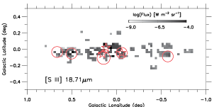
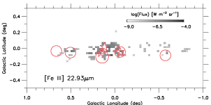
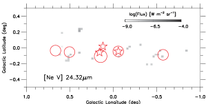
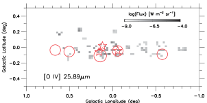
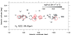
Figure 7.— Cont’d.

Table 2Line Flux Measurements from Individual Spectra

Galactic	Galactic	[Ne II]	H2 S(1)	[S III]	H2 S(0)	[S III]	[Si II]
longitude	latitude	$12.81\ \mu$m	$17.04\ \mu$m	$18.71\ \mu$m	$28.22\ \mu$m	$33.48\ \mu$m	$34.82\ \mu$m
(deg)	(deg)
$-0.7954$	$-0.0263$	$7.32\pm 0.11$	$8.67\pm 0.08$	$2.87\pm 0.15$	$1.99\pm 0.15$	$4.25\pm 0.14$	$16.88\pm 0.20$
$-0.8254$	$-0.0419$	$10.94\pm 0.13$	$8.10\pm 0.09$	$10.21\pm 0.17$	$1.87\pm 0.13$	$16.04\pm 0.35$	$25.87\pm 0.45$
$-0.8037$	$-0.0450$	$4.99\pm 0.11$	$6.83\pm 0.08$	$2.01\pm 0.15$	$1.68\pm 0.05$	$3.42\pm 0.11$	$11.57\pm 0.16$
$-0.8198$	$-0.0212$	$8.10\pm 0.11$	$6.65\pm 0.07$	$3.99\pm 0.22$	$1.46\pm 0.10$	$6.64\pm 0.11$	$15.18\pm 0.32$
$-0.7488$	$-0.0254$	$4.43\pm 0.13$	$5.13\pm 0.18$	$1.91\pm 0.23$	$1.60\pm 0.10$	$3.68\pm 0.18$	$7.82\pm 0.16$
$-0.7814$	$-0.0477$	$5.51\pm 0.20$	$9.42\pm 0.42$	$2.93\pm 0.34$	$2.08\pm 0.07$	$3.54\pm 0.31$	$11.85\pm 0.19$
$-0.7594$	$-0.0510$	$6.50\pm 0.18$	$9.64\pm 0.56$	$3.41\pm 0.54$	$2.75\pm 0.15$	$4.65\pm 0.40$	$13.44\pm 0.27$
$-0.7720$	$-0.0227$	$7.00\pm 0.18$	$10.87\pm 0.33$	$0.00\pm 0.00$	$2.38\pm 0.09$	$5.50\pm 0.34$	$14.19\pm 0.21$
$-0.7529$	$-0.0297$	$25.84\pm 0.70$	$54.67\pm 0.95$	$44.04\pm 2.32$	$13.19\pm 0.60$	$28.87\pm 1.07$	$58.81\pm 1.89$
$-0.7836$	$-0.0515$	$6.07\pm 0.10$	$9.02\pm 0.09$	$2.38\pm 0.15$	$1.98\pm 0.07$	$3.50\pm 0.59$	$12.99\pm 0.71$

Note. — Fluxes are corrected for dust extinction based on the Simpson et al. (2007) technique (see text), and are presented in units of $10^{-7}$ W m${}^{-2}\ {\rm sr}^{-1}$. Only those detected at more than $3\sigma$ are shown in this table.

Note. — Table 2 is published in its entirety in the electronic edition of the Astrophysical Journal Supplement Series. A portion is shown here for guidance regarding its form and content. The electronic edition of Table 2 contains the observed fluxes and errors for the emission lines listed in Table 1.

Table 3 lists the line fluxes measured by coadding all GC spectra, with three different extinction correction methods. The line fluxes and ratios listed in the second column are those measured from a spectrum coadded from individual spectra that have first been corrected for extinction using the Simpson et al. (2007) $F_{14}/F_{10}$ technique. Similarly, values in the third column are those measured in a spectrum coadded from individual spectra that were first corrected using the Schultheis et al. (2009) extinction map. The last column lists line fluxes and ratios measured by coadding all GC spectra, then applying an extinction correction for $\tau_{9.7}=3.439$ (the median value obtained from the Simpson et al. (2007) $F_{14}/F_{10}$ technique; see Figure 5).

Table 3Line Flux Measurements from Coadded Spectra

	Extinction Correction
Line Flux	Simpson et al. (2007)	Schultheis et al. (2009)	Posterior Correction
(Line Ratio)	($10^{-7}$ W m${}^{-2}\ {\rm sr}^{-1}$)	($10^{-7}$ W m${}^{-2}\ {\rm sr}^{-1}$)	($10^{-7}$ W m${}^{-2}\ {\rm sr}^{-1}$)
[S IV] $10.51\ \mu$m	$2.30\pm 3.22$	$0.00\pm 2.90$	$0.54\pm 4.38$
H2 S(2) $12.28\ \mu$m	$7.06\pm 0.34$	$8.45\pm 0.34$	$6.28\pm 1.60$
H I 7-6 $12.37\ \mu$m	$1.67\pm 0.17$	$1.95\pm 0.17$	$1.36\pm 0.75$
[Ne II] $12.81\ \mu$m	$58.09\pm 0.30$	$63.00\pm 0.32$	$45.94\pm 1.23$
[Ne V] $14.32\ \mu$m	$0.00\pm 0.08$	$0.00\pm 0.08$	$0.06\pm 0.32$
[Cl II] $14.37\ \mu$m	$0.32\pm 0.20$	$0.33\pm 0.09$	$0.22\pm 0.37$
[Ne III] $15.56\ \mu$m	$4.74\pm 0.26$	$4.94\pm 0.26$	$3.80\pm 1.48$
H2 S(1) $17.04\ \mu$m	$20.57\pm 0.25$	$24.90\pm 0.30$	$15.43\pm 2.28$
[S III] $18.71\ \mu$m	$89.87\pm 0.56$	$99.51\pm 0.67$	$52.91\pm 2.54$
[Fe III] $22.93\ \mu$m	$4.12\pm 0.19$	$4.05\pm 0.18$	$2.69\pm 1.39$
[Ne V] $24.32\ \mu$m	$0.23\pm 0.19$	$0.23\pm 0.25$	$0.16\pm 1.80$
[O IV] $25.89\ \mu$m	$0.70\pm 0.12$	$0.86\pm 0.13$	$0.60\pm 0.45$
[Fe II] $25.99\ \mu$m	$2.97\pm 0.12$	$3.48\pm 0.14$	$2.26\pm 0.83$
H2 S(0) $28.22\ \mu$m	$3.25\pm 0.59$	$3.85\pm 0.61$	$2.73\pm 1.27$
[S III] $33.48\ \mu$m	$75.30\pm 0.98$	$77.48\pm 1.03$	$58.07\pm 0.77$
[Si II] $34.82\ \mu$m	$61.76\pm 1.34$	$70.83\pm 1.41$	$51.29\pm 1.04$
[Ne III] / [Ne II]	$0.082\pm 0.005$	$0.078\pm 0.004$	$0.083\pm 0.032$
[Si II] / [S III]	$0.820\pm 0.021$	$0.914\pm 0.022$	$0.883\pm 0.021$
[Fe II] / [Ne II]	$0.051\pm 0.002$	$0.055\pm 0.002$	$0.049\pm 0.018$
[O IV] / [Ne II]	$0.012\pm 0.002$	$0.014\pm 0.002$	$0.013\pm 0.010$
[Fe II] / [O IV]	$4.228\pm 0.766$	$4.071\pm 0.624$	$3.766\pm 3.120$

Mapping results in Figure 7 are shown in the same order of increasing wavelength as in Table 1. Each pixel in the map covers a $1.5\arcmin\times 1.5\arcmin$ region of the sky ($\sim 3.5$ pc $\times 3.5$ pc), which is an order of magnitude larger than the area covered by a slit entrance of either SH or LH. We divided each extracted line flux by the areal coverage of the corresponding slit entrance ($53\ {\rm arcsec}^{2}$ for SH and $248\ {\rm arcsec}^{2}$ for LH), and computed unweighted mean intensities (W m^-2 sr^-1) in each pixel of the map in Figure 7. Each pixel includes two background IRS pointings on average.

Average line intensities in Figure 7 were corrected for foreground dust extinction derived using the Simpson et al. (2007) method (§ 2.3), which relies on the continuum flux ratio between $10\ \mu$m and $14\ \mu$m (see the top panel in Figure 4). Mid-IR forbidden emission lines, such as [Ne II] $12.81\ \mu$m, [Ne III] $15.56\ \mu$m, [S III] $18.71\ \mu$m, [S III] $33.48\ \mu$m, and [Si II] $34.82\ \mu$m, are strong in the CMZ. Their line strengths vary across the region, with strongest emission observed near the Arches cluster and Sgr B1. Weaker emission is observed in the CMZ for H I 7–6 12.37 $\mu$m, [Cl II] 14.37 $\mu$m, [Fe III] 22.93 $\mu$m, and [Fe II] 25.99 $\mu$m. Emission from pure rotational H₂ lines, 0–0 S(0), 0–0 S(1), and 0–0 S(2) at $28.22\ \mu$m, $17.04\ \mu$m, and $12.28\ \mu$m, respectively, is also strong, but these H₂ lines are relatively constant over the CMZ. We will discuss the uniform H₂ emission in § 3.2, further utilizing radial velocities measured from the IRS spectra. Fine structure lines from highly ionized species such as [O IV] $25.89\ \mu$m are found throughout the CMZ, but [S IV] 10.51 $\mu$m, [Ne V] $14.32\ \mu$m and [Ne V] $24.32\ \mu$m were detected only in a few lines of sight to the GC. Our mapping results and interpretation remain qualitatively unchanged if the Schultheis et al. (2009) map is used for the foreground extinction correction.

3.2. Molecular Hydrogen Line Emission and Radial Velocity Mapping

Figure 7 shows line intensity maps for pure rotational transitions from the lowest three levels of molecular hydrogen, H₂ S(2) $12.28\ \mu$m, S(1) $17.04\ \mu$m, and S(0) $28.22\ \mu$m. We detected these lines in almost all lines of sight in the GC at more than a $3\sigma$ level. Their intensity distributions are rather uniform in the CMZ, compared to the spatial structures seen for ionic forbidden emission lines. We also find weak correlations in line intensities between the pure rotational hydrogen emission and ionic forbidden lines ($0.3\lesssim p\lesssim 0.6$); correlations are stronger ($p\gtrsim 0.9$) among strong forbidden emission lines.

The pure rotational H₂ lines from warm molecular gas are important tools for studying heating mechanisms in the GC (e.g., see Roussel et al., 2007, for extragalactic H₂ line measurement). Rodríguez-Fernández et al. (2004) suggested that a combination of PDRs and diffuse ionized gas can be used to explain the observed dust, H₂, neutral gas, and ionized gas emission in the GC. Pak et al. (1996) also found that the most likely cause of the large-scale ro-vibrational H₂ $\nu=1\rightarrow 0$ S(1) emission at $2.12\ \mu$m in the GC is UV excitation by hot massive stars. However, Rodríguez-Fernández & Martín-Pintado (2005) showed that while PDR models can reproduce the observed pure rotational H₂ lines from excited levels in the GC, they are not enough to explain all the emission from the lowest levels, S(0) and S(1). They argued that low velocity shocks or turbulent motions are needed as an additional heating mechanism to reproduce excess emission from low excitation H₂ lines. On the other hand, Simpson et al. (2007) concluded, based on their H₂ rotational line measurements, that multi-component models of warm molecular gas in PDRs along the line of sight to the GC can fully explain the observed H₂ line ratios, without requiring shocks.

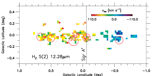
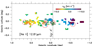
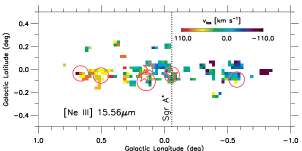
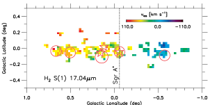
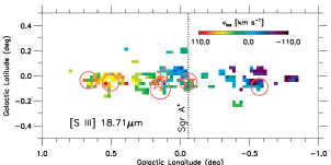
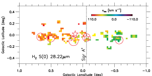
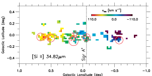
Figure 8.— Panoramic radial velocity maps of the GC, constructed from strong ionic and molecular hydrogen emission lines. The vertical line indicates the Galactic longitude of Sgr A* at the dynamical center of the Galaxy. The sense of the rotation is that the eastern part of the GC, including the Sgr B complex, is systematically receding from the Sun (positive $v_{r}$), consistent with the rotation of the Galactic disk. Each pixel covers $1.5\arcmin\times 1.5\arcmin$ ($\sim 3.5$ pc $\times 3.5$ pc). Key features of the GC are overlaid (see Figure 1).

To further investigate the source of low-level rotational H₂ lines, we compared radial velocity distributions of various mid-IR emission lines. Figure 8 shows panoramic radial velocity ($v_{r}$) maps of the CMZ for several strong ionic and molecular hydrogen emission lines. Radial velocities from strong ionic lines exhibit a systematic rotation of the CMZ, consistent with the rotation of the Galactic disk. The sense of the rotation is that the eastern part of the GC, including the Sgr B complex, is systematically receding from the Sun (positive $v_{r}$), and the Sgr C complex is systematically approaching the Sun (negative $v_{r}$), with respect to the dynamical center of the Galaxy, indicated by a vertical dotted line at Sgr A*.

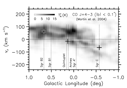
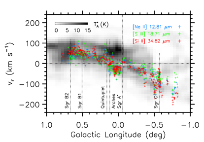
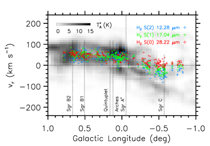
Figure 9.— Top: Average antenna temperatures (T${}^{*}_{A}$) at $|b|<0.1\arcdeg$ from CO $J=4\rightarrow 3$ survey (Martin et al., 2004). Large cross signs indicate radial velocities from radio recombination-line studies: de Pree et al. (1996, Sgr B2), Lang et al. (2001, Arches cluster), and Liszt & Spiker (1995, Sgr C). Middle: Radial velocities from strong forbidden emission lines, at $|b|<0.1\arcdeg$, on top of the CO $l$-$v$ diagram. Bottom: Radial velocities from molecular hydrogen lines, on top of the CO $l$-$v$ diagram. Vertical dotted lines indicate Galactic longitudes of several landmarks in the CMZ.

Radial velocity distributions as a function of Galactic longitude are displayed in Figure 9, on top of the $l$-$v_{r}$ diagram of CO $J=4\rightarrow 3$ (Martin et al., 2004); see § 2.2 for details on the $v_{r}$ determination. Only those $v_{r}$ measurements near the Galatic plane, $|b|<0.1\arcdeg$, are included in the $l$-$v_{r}$ diagrams, and averaged antenna temperatures ($T^{*}_{A}$) from the CO survey are shown in the same latitude range.

Three large cross signs in the upper panel of Figure 9 indicate radial velocities from radio recombination-line studies (de Pree et al., 1996; Lang et al., 2001; Liszt & Spiker, 1995), independent of the $v_{r}$ measurement in Mehringer et al. (1992). These show an excellent agreement with our $v_{r}$ values from ionic lines (middle panel). The IRS ionic lines generally follow a lower branch (smaller $v_{r}$) in the CO $l$-$v_{r}$ diagram, and the highly negative radial velocities observed in the northern rim of Sgr A are associated with the Arched Filaments and the Radio Bubble (e.g., Simpson et al., 2007). The IRS spectral resolution is not high enough to resolve individual radial velocity structures along the line of sight as in the CO survey, and our $v_{r}$ measurements refer to those that belong to the highest peak of the emission.

Radial velocities from the molecular hydrogen lines S(0), S(1), and S(2) are displayed in the bottom panel of Figure 9. As shown in this panel, H₂ lines show a systematically flatter $v_{r}$ curve than those from forbidden lines (middle panel). The flatness of the $v_{r}$ curve depends on H₂ excitation, with S(0) showing the most difference from [Ne II] and S(2) showing the least. The H₂ velocities and [Ne II] velocities differ most in the region between the Arches cluster and Sgr A, and toward Sgr C. Simpson et al. (2007) also found a systematically different $v_{r}$ between ionized species and molecular hydrogen. Our mapping results show that $v_{r}$ from the lowest H₂ energy level, S(0), even exhibits flat rotation near Sgr A*. A flat $v_{r}$ distribution in the longitude vs. radial velocity diagram toward the GC is typically attributed to gas clouds in the disk along the line of sight to the GC (e.g., Binney et al., 1991; Rodríguez-Fernández et al., 2006). This suggests that the H₂ line-emitting clouds are a superposition of several dense clouds along the line of sight to the GC. The $v_{r}$ offsets for H₂ emission lines are still uncertain, because we opted to use the CO $J=4\rightarrow 3$ data cube (Martin et al., 2004) at a particular longitude range, $-0.2\arcdeg<l<+1.0\arcdeg$ (see § 2.2).

Both the uniform H₂ intensity distributions and distinct H₂ radial velocity structures suggest that a significant fraction of the S(0) emission, and a smaller fraction of S(1) and S(2) emission, arise in clouds that are probably not associated with the mid-IR forbidden line emitting cloud complexes in the CMZ.

3.3. Emission Line Ratio Mapping in the GC

Mapping results for forbidden line ratios are presented in Figure 10. Line fluxes with extinction corrections from the Simpson et al. (2007) $F_{14}/F_{10}$ technique were used in the computation of these line ratios, and only those detected at more than a $3\sigma$ level were included in Figure 10. A moving boxcar average for these line ratios is shown on the right panels as a function of the Galactic longitude, where the error bars indicate the standard deviation of data points in each longitude bin. We also present moving boxcar-averaged line ratios with extinction corrections from the Schultheis et al. (2009) map (dashed green line) and without any correction for extinction (dashed grey line). The [S III] 18.71 $\mu$m / [S III] 33.48 $\mu$m line ratio is strongly affected by extinction, as Simpson et al. (2007) also found, and we therefore move the discussion of this line ratio to the Appendix. All of the other line ratios in Figure 10 are insensitive to the extinction correction, and will be discussed in the following sections.

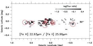
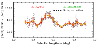
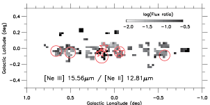
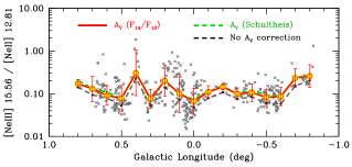
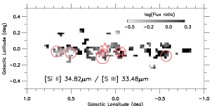
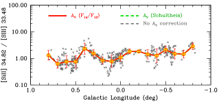
Figure 10.— Panoramic maps of line intensity ratios in the GC (left) and corresponding line ratios as a function of Galactic longitude (right). Only those lines detected at more than a $3\sigma$ level are included in the above mapping of average line ratios within each $1.5\arcmin\times 1.5\arcmin$ ($\sim 3.5$ pc $\times 3.5$ pc) pixel. Line ratios are corrected for foreground extinction based on the ratio between $10\ \mu$m and $14\ \mu$m continuum fluxes ($F_{14}/F_{10}$; see the top panel in Figure 4). Moving averaged points are connected with a solid red line, where error bars indicate a $1\sigma$ dispersion in each moving average box. Green dashed lines are moving averaged flux ratios assuming the Schultheis et al. (2009) extinction map, and the grey dashed lines are the data without extinction corrections. Key features of the GC are overlaid in the left panels (see Figure 1). Horizontal dotted line at [S III] $18.71\ \mu$m / [S III] $33.48\ \mu$m $=0.4$ represents the theoretical lower limit, where the gas electron density ($n_{e}$) approaches zero (Rubin, 1989).

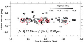
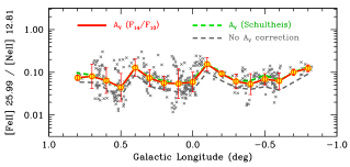
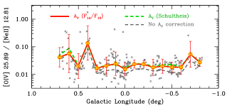
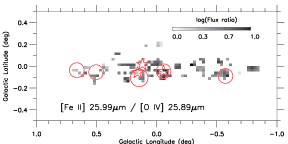
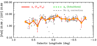
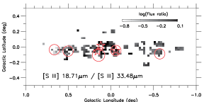
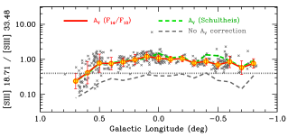
Figure 10.— Cont’d.

We illustrate the distribution of [Fe III] $22.93\ \mu$m / [Fe II] $25.99\ \mu$m as a function of Galactic longitude in Figure 10. This line ratio shows a broad peak centered at $l\sim+0.15\arcdeg$, near the Quintuplet and Arches clusters of massive stars and the Radio Bubble. The [Fe III] $22.93\ \mu$m / [Fe II] $25.99\ \mu$m ratio is not sensitive to the hardness of the ionizing radiation field, as [Ne III] $15.56\ \mu$m / [Ne II] $12.81\ \mu$m is (see below). Instead, it is sensitive to the ionization parameter, $U$, which is the ratio of the photoionization rate to the recombination rate (Contini, 2009). This is because [Fe III] $22.93\ \mu$m, with an ionization potential of $16.2$ eV, only arises in ionized gas, while [Fe II] $25.99\ \mu$m, with an ionization potential of $7.9$ eV, can arise both from neutral and ionized gas (Kaufman et al., 2006). Comparisons of models with previous GC ISM observations have found $-3\leq\log(U)\leq-1$ (Rodríguez-Fernández & Martín-Pintado, 2005; Contini, 2009).

4. Comparison with Nearby Galaxies

In this section, we compare ratios of ionic lines mapped in the GC to ratios measured in the Spitzer Infrared Nearby Galaxies Survey (SINGS) (Dale et al., 2009). The SINGS sample (Kennicutt et al., 2003) contains 75 galaxies, evenly distributed among elliptical, spiral, and irregular galaxies, and including a range of nuclear activity (quiescent, starburst, LINER, Seyfert). The SINGS galaxies have a median distance of $9.5$ Mpc, and the closest is at $0.6$ Mpc. The IRS SH and LH slits correspond to $14$ pc $\times 33$ pc and $32$ pc $\times 65$ pc, respectively, for a galaxy at $0.6$ Mpc; they cover $220$ pc $\times 520$ pc and $510$ pc $\times 1000$ pc, respectively, for a galaxy at $9.5$ Mpc. By comparison, we bin our GC line data into $1.5\arcmin\times 1.5\arcmin$ pixels ($3.5$ pc $\times 3.5$ pc). Our coadded spectrum of the CMZ is constructed from spectra across a $210$ pc $\times 60$ pc region, which is a good match to the SINGS spatial resolution.

4.1. Radiation Field Hardness and Oxygen Abundance

The [Ne III] $15.56\ \mu$m / [Ne II] $12.81\ \mu$m line ratio is a useful indicator of the radiation field hardness for star-forming regions, as this ratio is higher when stars are hotter. The mapping results for this line ratio are included in Figure 10. As shown in this map, the highest excitation gas traced by [Ne III]/[Ne II] ratio is peaked in the Radio Bubble and Quintuplet cluster, where ionizing photons from newly born massive stars in the Quintuplet cluster are most likely responsible for the hard radiation field. Simpson et al. (2007) also found the same result along the $l\approx 0.1\arcdeg$ stripe (see also Rodríguez-Fernández & Martín-Pintado, 2005). The mean line ratio ($\approx 0.1$–$1$) is consistent with recent bursts of massive star formation in this region in the last few million years (e.g., Thornley et al., 2000; Rodríguez-Fernández & Martín-Pintado, 2005), and is insensitive to a choice of foreground extinction corrections (see dashed lines in Figure 10).

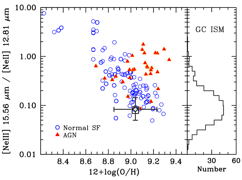
Figure 11.— Modification of Figure $4$ in Dale et al. (2009), displaying [Ne III] $15.56\ \mu$m / [Ne II] $12.81\ \mu$m as a function of oxygen abundance for nuclear and extra-nuclear star-forming regions (open blue circles) in the Spitzer Infrared Nearby Galaxies Survey (SINGS). AGNs are shown as red filled triangles. The number distribution of GC spectra in [Ne III]/[Ne II] is shown in the right panel. Filled diamond point represents a median line ratio at the GC, plotted at the oxygen abundance, $[12+\log{({\rm O/H})}]=9.04\pm 0.19$, measured in GC stellar photospheres (Cunha et al., 2007). The vertical error bars indicate the interquartile range of line ratios measured in the GC. Open box shows the line flux ratio from the coadded GC spectrum.

The [Ne III] / [Ne II] ratio also depends on the nebular oxygen abundance, [O/H]. Figure 11 is a modification of Figure $4$ in Dale et al. (2009), which shows [Ne III]/[Ne II] measured from a sample of normal star-forming regions (both nuclear and extra-nuclear; open blue circles) in SINGS. As shown in Figure 11, the line ratio decreases as the nebular oxygen abundance increases in these normal extragalactic star-forming regions, because the UV stellar spectrum of ionizing hot stars depends on the (photospheric) metal abundance. Active galactic nuclei (AGNs) are also displayed as red filled triangles, but they do not follow the line ratio vs. abundance trend observed among extra-galactic star-forming regions.

The median [Ne III] / [Ne II] ratio ($\approx 0.08$) measured in the GC is shown as a filled diamond point in Figure 11, and the number distribution of GC spectra is displayed in the right panel. The vertical error bars indicate the interquartile range of line ratios measured in the GC ($=0.05$–$0.14$). The line ratios from the coadded spectrum (Table 3), shown as an open box symbol, are consistent with the median value within the interquartile ranges. The [Ne III] / [Ne II] line ratio of the CMZ in Figure 11 is plotted at the stellar oxygen abundance, $[12+\log{({\rm O/H})}]=9.04\pm 0.19$ (Cunha et al., 2007), which was derived from high-resolution infrared spectroscopy of five luminous cool stars within $30$ pc of the GC. Their abundance measurement is consistent with Davies et al. (2009), who measured $[12+\log{({\rm O/H})}]=9.09\pm 0.11$ from a star that was not included in Cunha et al. (2007). Figure 11 demonstrates that the CMZ follows the abundance vs. [Ne III] / [Ne II] trend observed in normal star-forming regions in nearby galaxies. This implies that the hardness of the stellar energy distribution in the GC is similar to those found in nuclear and extra-nuclear star-forming environments, assuming that the nebular oxygen abundance [O/H] is close to what was measured from stars in the GC.

4.2. AGN vs. Normal Star-Forming Activities in the GC

Empirical evidence suggests that some mid-IR line ratios are useful diagnostic tools for discriminating between normal star-forming regions and AGNs (Lutz et al., 1998; Sturm et al., 2006; Dale et al., 2009). In this section, we use several of these emission-line diagnostics, such as [Si II] $34.82\ \mu$m / [S III] $33.48\ \mu$m and [O IV] $25.89\ \mu$m / [Ne II] $12.81\ \mu$m, to study properties of gas clouds in the CMZ. We inspect these line ratios in our GC spectra, both separately and as a whole, and compare results with those observed in other nearby galaxies.

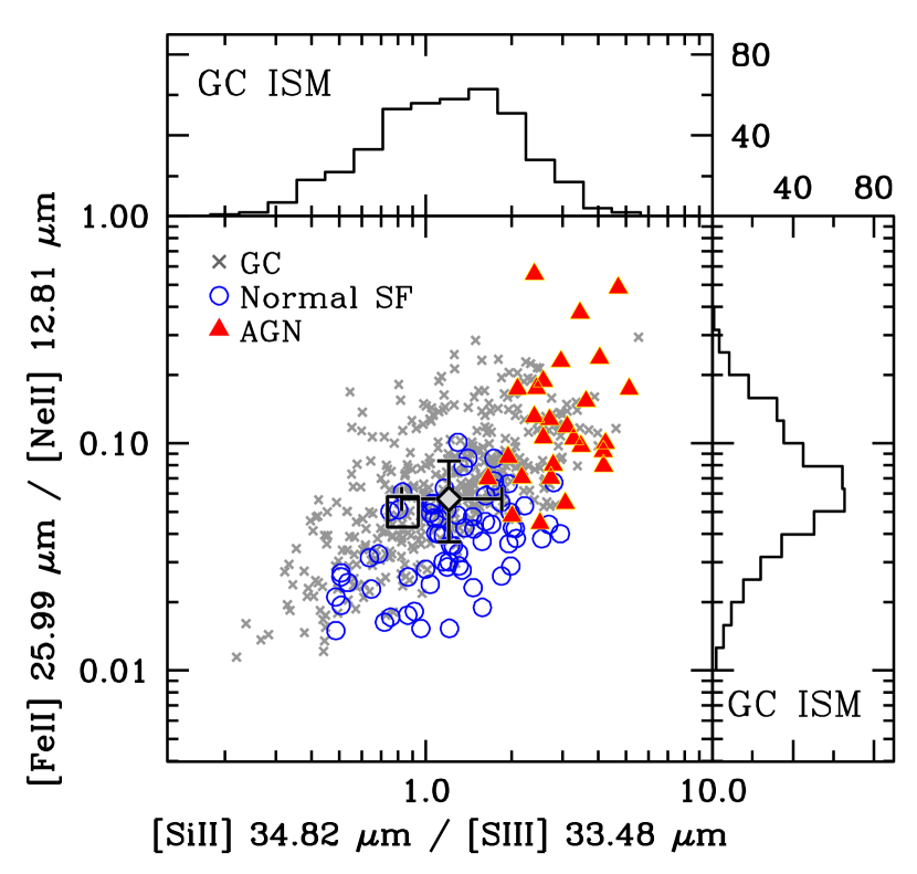
Figure 12.— Modification of Figure $6$ in Dale et al. (2009), showing [Si II] $34.82\ \mu$m / [S III] $33.48\ \mu$m vs. [Fe II] $25.99\ \mu$m / [Ne II] $12.81\ \mu$m. Normal star-forming regions (both nuclear and extra-nuclear) and AGNs are displayed as open blue circles and filled red triangles, respectively. Grey points are individual GC spectra, and their number distributions are shown on each axis. Filled diamond point represents median line ratios in the CMZ, with interquartile ranges of line ratios indicated by error bars. Open box shows the line flux ratio from the coadded GC spectrum.

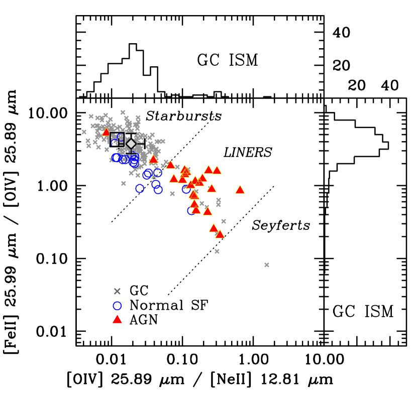
Figure 13.— Same as in Figure 12, but for [O IV] $25.89\ \mu$m / [Ne II] $12.81\ \mu$m vs. [Fe II] $25.99\ \mu$m / [O IV] $25.89\ \mu$m. Two dashed diagonal lines show approximate divisions from Sturm et al. (2006) into values for starbursts, LINERs (or pure shocks), and Seyferts (see their Figure 2).

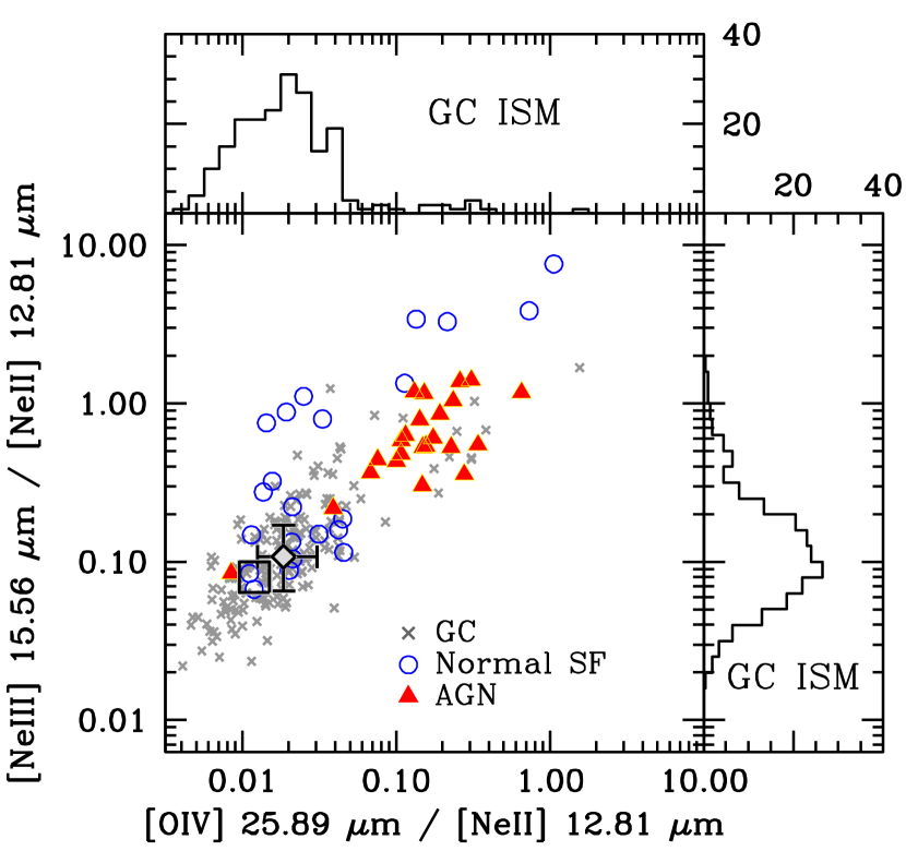
Figure 14.— Same as in Figure 12, but for [O IV] $25.89\ \mu$m / [Ne II] $12.81\ \mu$m vs. [Ne III] $15.56\ \mu$m / [Ne II] $12.81\ \mu$m.

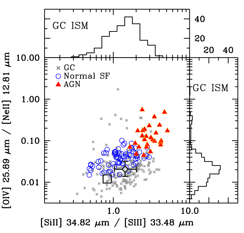
Figure 15.— Same as in Figure 12, but for [Si II] $34.82\ \mu$m / [S III] $33.48\ \mu$m vs. [O IV] $25.89\ \mu$m / [Ne II] $12.81\ \mu$m.

4.2.1 [Si II]/[S III] and [Fe II]/[Ne II]

Figure 12, which is a modification of Figure $6$ in Dale et al. (2009), is one of such diagnostic tools, showing [Si II] $34.82\ \mu$m / [S III] $33.48\ \mu$m vs. [Fe II] $25.99\ \mu$m / [Ne II] $12.81\ \mu$m from SINGS. Both nuclear and extra-nuclear star-forming regions are shown as blue circles, and AGNs are shown as red filled triangles. Previous theoretical work showed that the [Si II] $34.82\ \mu$m line can be emitted either from PDRs or H II regions, while [S III] $33.48\ \mu$m is mostly from H II regions (Kaufman et al., 2006).

In Figure 12, normal star-forming regions show a strong correlation between [Si II] $34.82\ \mu$m / [S III] $33.48\ \mu$m and [Fe II] $25.99\ \mu$m / [Ne II] $12.81\ \mu$m, the latter being another useful line diagnostic of the ionization parameter. However, AGNs generally show higher values of these line ratios than values from normal star-forming nuclear and extra-nuclear regions in nearby galaxies, and a combination of these two IR line ratios separates AGNs and normal star-forming regions relatively well. Physical reasons for this empirical division are debated, but must include the low ionization potentials of Si⁺ and Fe⁺ ions ($8.15$ eV and $7.90$ eV, respectively) and the higher ionization potentials of Ne⁺ and S⁺⁺ ($21.56$ eV and $23.34$ eV, respectively). Dale et al. (2009) proposed a number of possible physical mechanisms for the observed separation between AGNs and normal star-forming regions, which include (1) enhanced dust destruction and sublimation of refractory elements (Si and Fe) in the harsh AGN environment, (2) extended low-ionization volumes in AGNs produced by X-ray photo-ionization processes, and/or (3) enhanced line emission from [Si II] $34.82\ \mu$m and [Fe II] $25.99\ \mu$m due to high gas density in PDRs and/or X-ray dominated regions in AGNs.

Gray cross points in Figure 12 display line ratios measured from individual GC spectra, shown only for those detected at more than a $3\sigma$ significance. Their number distributions are shown in a histogram on each axis. The filled diamond point represents the median line ratio from the individual spectra of the entire CMZ ([Si II] / [S III] $=1.21$ and [Fe II] / [Ne II] $=0.06$), with error bars indicating interquartile ranges. The values from the coadded CMZ spectrum are shown as an open box symbol; they are different from the median GC values because we only plot $3\sigma$ detections. Clearly, the vast majority of the GC measurements and the median GC values are found in an area that is mostly populated by normal star-forming regions in nearby galaxies. Line ratios on both axes are insensitive to extinction corrections.

4.2.2 [O IV]/[Ne II] , [Fe II]/[O IV], and [Ne III]/[Ne II]

Another set of mid-IR line diagnostics to separate AGNs from normal star-forming regions are displayed in Figure 13, which plots [O IV] $25.89\ \mu$m / [Ne II] $12.81\ \mu$m vs. [Fe II] $25.99\ \mu$m / [O IV] $25.89\ \mu$m, and in Figure 14, which shows [O IV] $25.89\ \mu$m / [Ne II] $12.81\ \mu$m vs. [Ne III] $15.56\ \mu$m / [Ne II] $12.81\ \mu$m. Both diagrams, which involve line emission from [O IV] $25.89\ \mu$m, separate AGNs (red filled triangles) from normal star-forming regions (blue open circles) relatively well; see Dale et al. (2009) for the SINGS targets used in these diagrams. In addition, two diagonal dashed lines in Figure 13 show approximate divisions between starbursts, LINERs (Low Ionization Nuclear Emission Regions) and pure shocks, and Seyfert galaxies from Sturm et al. (2006, see their Figure 2). Figure 14 shows that there are a few normal star-forming regions from SINGS (blue circles) with [O IV] $25.89\ \mu$m / [Ne II] $12.81\ \mu$m greater than $\sim 0.10$. These are low-metallicity star-forming regions, as revealed from the comparison between Figure 11 and Figure 14, where strong [O IV] $25.89\ \mu$m emission is due to a harder spectrum for the stellar ionizing photons in low-metallicity environments.

Gray cross points in Figures 13–14 represent our measurements from individual GC spectra. As in Figure 12, we only included emission lines with more than $3\sigma$ detections. Number distributions of ionic line ratios are shown on each axis. The median values from the individual spectra of the CMZ are indicated by a grey diamond point; error bars represent the interquartile ranges of distributions of individual GC spectra. The line ratios for the coadded GC spectrum is displayed as an open box. Figures 13–14 show that the emission-line properties of the CMZ are similar to those of extragalactic star-forming regions (blue circles) and starburst galaxies (upper left corner in Figure 13, fenced with a dashed diagonal line). This agrees with our conclusion based on [Si II] / [S III] vs. [Fe II] / [Ne II] diagnostics in Figure 12.

The line ratios for the coadded spectrum of the CMZ in Figure 14 ([O IV]/[Ne II]$\sim 0.01$ and [Ne III]/[Ne II]$\sim 0.08$) are found within the range observed among starburst galaxies (Lutz et al., 1998, see their Figure 2). Lutz et al. (1998) suggested that shocks and/or hot stars are the likely origins of [O IV] observed in these galaxies, rather than buried AGNs. Simpson et al. (2007) also reported widespread detection of [O IV] in the GC; they attributed this to shocks in the CMZ (see also Contini, 2009). Simpson et al. (2007) further argued for the existence of shocked gas inside of the Radio Bubble based on the high Fe abundance there, since grain destruction in shocks can return Fe to the ISM.

If the above result implies the importance of shocked gas in the GC, widespread detections of highly ionized ions such as [O IV] (Figure 7) may support a large scale origin of turbulent motions in the GC. In other words, the relatively uniform intensity distributions of these lines in our mapping suggest that conditions for producing the lines are common throughout the CMZ. One likely explanation is a dissipation of supersonic turbulence ($\gtrsim 10$ km/s in the CMZ) induced by differential Galactic rotation or shearing motion of clouds in the GC (e.g., Wilson et al., 1982; Guesten et al., 1985). However, shocks created by massive stars are also likely; see Rodríguez-Fernández et al. (2004) for discussion of other potential heating mechanisms, such as cosmic rays, magnetic heatings, or X-ray dominated regions.

While most of the GC points (gray crosses) in Figure 12 are found in an area occupied by normal star-forming regions, including the coadded spectrum of the CMZ, about $10\%$ of the detections fall into AGN territory. As shown in the mapping results in Figure 10, both [Si II] $34.82\ \mu$m / [S III] $33.48\ \mu$m and [Fe II] $25.99\ \mu$m / [Ne II] $12.81\ \mu$m line ratios are peaked near Sgr A and the north-western rim of Sgr B. The scatter of the [Fe II] $25.99\ \mu$m / [Ne II] $12.81\ \mu$m points in the moving average plot is larger than that of [Si II] $34.82\ \mu$m / [S III] $33.48\ \mu$m because [Fe II] $25.99\ \mu$m is relatively weak and blended with [O IV] $25.89\ \mu$m. Nevertheless, the observed systematic trend in Galactic longitude (right panels in Figure 10) is larger than the random scatter of data points, which means that those GC points in the upper right corner in Figure 12 are not entirely produced by a statistical fluctuation.

Figures 13 and 14 show that about 10% of individual GC spectra fall in the AGN (red filled triangles) region of these line ratio diagrams, almost independent of the choice of extinction correction. Note again that a few SINGS targets from extragalactic star-forming regions are also found in the area denoted as AGNs in Figure 14, because of their low metal abundance (see above). On the other hand, the GC spectra with strong [O IV] $25.89\ \mu$m / [Ne II] $12.81\ \mu$m are not due to a low metallicity environment, because they follow the AGN sequence in Figure 14 rather than that of metal-poor, star-forming regions, and because the GC has a supersolar oxygen abundance (Cunha et al., 2007; Davies et al., 2009).

If high values of [O IV] $25.89\ \mu$m / [Ne II] $12.81\ \mu$m and low values of [Fe II] $25.99\ \mu$m / [O IV] $25.89\ \mu$m in Figures 13 are due to ionization by a power-law continuum source (i.e., an AGN), then the empirical division in Figure 12 leads to a conclusion that these same spectra should also have high values of the ratios of [Si II] $34.82\ \mu$m / [S III] $33.48\ \mu$m and [Fe II] $25.99\ \mu$m / [Ne II] $12.81\ \mu$m. To answer the question of whether AGN-like points in Figures 12–14 are from the same individual GC spectra, we plot [Si II] $34.82\ \mu$m / [S III] $33.48\ \mu$m vs. [O IV] $25.89\ \mu$m / [Ne II] $12.81\ \mu$m in Figure 15. We also plot these line ratios measured in the coadded CMZ spectrum, and compare to the line ratios measured in star-forming galaxies and AGNs (Dale et al., 2009).

We find that only $3\%$ of GC points fall in the AGN-like region of Figure 15. Virtually all GC data points have ratios of [Si II] $34.82\ \mu$m / [S III] $33.48\ \mu$m and [O IV] $25.89\ \mu$m / [Ne II] $12.81\ \mu$m agreeing with the line ratios observed in star-forming galaxies. The few points that are not similar to star-forming galaxies are those at high Galactic latitudes ($l\sim+0.4\arcdeg$, $b\sim+0.2\arcdeg$ and $l\sim+0.6\arcdeg$, $b\sim+0.2\arcdeg$).

We considered whether the positions with AGN-like line ratios could be due to having been irradiated by Sgr A* if it was in a more active state in the past. This idea has been suggested to explain bright Fe I K$\alpha$ emission at $6.4$ keV in Sgr B2 and other molecular clouds in the GC (Sunyaev et al., 1993; Koyama et al., 1996; Murakami et al., 2001). The Fe I K$\alpha$ emission in the GC varies spatially and temporily (Terrier et al., 2010). Capelli et al. (2012) analyzed the Fe I K$\alpha$ emission to derive a light curve for the X-ray luminosity of Sgr A* over the last several hundred years. Apparent superluminal motion has also been observed in $6.4$ keV Fe I K$\alpha$ emission (Ponti et al., 2010). Others argue, however, that widespread Fe I K$\alpha$ emission in the GC can be explained by cosmic rays (Yusef-Zadeh et al., 2007, 2013; Chernyshov et al., 2012; Tatischeff et al., 2012). Yusef-Zadeh et al. (2013) show, in their Figure 8a, an image of the equivalent width of Fe I K$\alpha$ emission, covering $-0.8\arcdeg<l<+0.7\arcdeg$ and $\pm 0.4\arcdeg$ in $b$. We compared this image to our Figure 10, an image of the [O IV]/[Ne II] line ratio in the GC ISM. We find no correlation between GC ISM positions with AGN-like line ratios and regions of enhanced Fe I K$\alpha$ emission. Our data do not support – but neither do they rule out – the idea that strong $6.4$ keV Fe I K$\alpha$ emission is caused by higher X-ray luminosity of Sgr A* in the past.

We conclude that our observations of mid-IR line emission in the central $210$ pc $\times 60$ pc of the Galaxy show no evidence of excitation by a power-law continuum. The few points that are not similar to star-forming galaxies are outliers, such as those excited by very hot sources (e.g., Wolf-Rayet stars, planetary nebulae, or X-ray binaries), rather than belonging to an AGN-like trend. Our results agree with those of Simpson et al. (2007) and Contini (2009), who conclude that the mid-IR line ratios in a smaller Spitzer data set can be explained by photoionization by hot stars, combined with shocks.

Figure 15 shows a significant offset between the median value of [O IV] $25.89\ \mu$m / [Ne II] $12.81\ \mu$m measured from individual GC spectra and the value from the coadded CMZ spectrum. Emission from [Ne II] $12.81\ \mu$m, [Si II] $34.82\ \mu$m, and [S III] $33.48\ \mu$m is detected in virtually all individual GC spectra. The offset, then, is due to faint [O IV] $25.89\ \mu$m emission which is missing from the number distribution for individual spectra (we only plot 3$\sigma$ detections) but which contributes to the coadded spectrum. Because the [O IV] $25.89\ \mu$m / [Ne II] $12.81\ \mu$m line ratio from the coadded spectrum is at the lower end of the range of GC line ratios on Figure 15, we can be confident that excluding regions of faint [O IV] $25.89\ \mu$m emission does not change our conclusion that the GC is similar to star-forming galaxies and not similar to AGNs.

5. Summary

We present a mid-IR spectroscopic survey of $428$ positions in the ISM of the CMZ using the Spitzer/IRS, and construct mid-IR emission line maps for several forbidden and molecular hydrogen lines over the CMZ. We derive both line strengths and radial velocities from individual lines, and compute line flux ratios as a probe of physical conditions in the GC. Our mapping is superior to previous survey results in terms of the total area covered in the GC. We also construct a CMZ spectrum by coadding individual spectra after correcting each for extinction.

Mid-IR emission lines from the pure rotational transitions of molecular hydrogen, S(0), S(1), and S(2), are observed in almost all lines of sight to the CMZ. Their intensity distribution in the GC is relatively uniform; their radial velocity distributions are poorly correlated with those from ionic species, with worse correlation for S(0) than S(2). We view this as evidence that most of the H₂ S(0) emission, and some of the S(1) and S(2) emission, arises from PDRs along the line of sight to the GC, rather than PDRs associated with ionized gas in the GC.

The radiation field hardness traced by the [Ne III] $15.56\ \mu$m / [Ne II] $12.81\ \mu$m line ratio indicates that the highest excitation gas clouds are found in the Radio Bubble region and Quintuplet cluster, and the mean value in the GC is consistent with a recent burst of star formation in the last few million years. The hardness of the ionization spectrum from hot stars is tied to the metal abundance of the star-forming clouds, and our GC spectra, combined with the published GC stellar oxygen abundance, show that the hardness of the GC exciting radiation is similar to that found in normal star-forming regions in nearby galaxies.

We present mid-IR line-ratio diagrams such as [Si II] $34.82\ \mu$m / [S III] $33.48\ \mu$m vs. [Fe II] $25.99\ \mu$m / [Ne II] $12.81\ \mu$m, [O IV] $25.89\ \mu$m / [Ne II] $12.81\ \mu$m vs. [Fe II] $25.99\ \mu$m / [O IV] $25.89\ \mu$m, [O IV] $25.89\ \mu$m / [Ne II] $12.81\ \mu$m vs. [Ne III] $15.56\ \mu$m / [Ne II] $12.81\ \mu$m, and [Si II] $34.82\ \mu$m / [S III] $33.48\ \mu$m vs. [O IV] $25.89\ \mu$m / [Ne II] $12.81\ \mu$m. We compare properties of individual GC spectra to those observed in nearby extragalactic star-forming regions and AGNs. These diagrams show that the individual GC spectra and the mean GC spectrum are consistent with normal star forming activity, where emission from highly ionized species such as [O IV] is likely produced by shocks and/or turbulence prevalent in the CMZ clouds. Our GC line ratios do not agree with line ratios observed for LINER galaxies or AGNs.

Appendix A [S III] $18.71\ \mu$m / [S III] $33.48\ \mu$m

Line ratios from the same ionized species such as [S III] $18.71\ \mu$m / $33.48\ \mu$m are generally sensitive to the electron gas density ($n_{e}$) with a weak dependence on the electron gas temperature (e.g., Rubin, 1989; Martín-Hernández et al., 2002; Dale et al., 2009). But [S III] $18.71\ \mu$m is found in the middle of the strong and broad $18\ \mu$m silicate feature, while [S III] $33.48\ \mu$m is almost unaffected by foreground absorption (see the bottom panel in Figure 2). Thus we, like Simpson et al. (2007), find that the [S III] $18.71\ \mu$m / $33.48\ \mu$m ratio is most useful for checking our foreground extinction correction.

The grey dashed line for the [S III] $18.71\ \mu$m and $33.48\ \mu$m ratio in the right panel of Figure 10 indicates the observed line intensity ratios without any extinction correction. These values are located below the lower limit set by the theoretical value ($0.4$; dotted horizontal line) as $n_{e}\rightarrow 0$ cm^-3 (Rubin, 1989). On the other hand, mean line ratios after extinction corrections using either the Simpson et al. (2007) method (red solid line) or the Schultheis et al. (2009) map (green dashed line) are higher than the theoretical limit, clearly showing a strong dependence of the line ratio on the foreground extinction correction.

Over most parts of the GC, the [S III] $18.71\ \mu$m / [S III] $33.48\ \mu$m ratios are close to unity after the extinction correction. This line ratio value corresponds to $n_{e}\sim 500$ cm^-3 (Martín-Hernández et al., 2002; Dale et al., 2009). Mean line ratios from either of the extinction estimation techniques used above are in excellent agreement with each other, and are relatively uniform across the CMZ. However, these average line ratios become lower than the minimum theoretical value ($\approx 0.4$) near Sgr B2. Sgr B2 has very high extinction (Figure 4), so we view this as due to unrecognized systematic errors in our extinction estimates from the Simpson et al. (2007) and Schultheis et al. (2009) approaches that greatly underestimated $\tau_{9.7}$ in this region. Goicoechea et al. (2004) found $n_{e}\sim 240\ {\rm cm^{-1}}$ in Sgr B2 based on ISO observations.

References

- An et al. (2009) An, D., Ramírez, S. V., Sellgren, K., et al. 2009, ApJ, 702, L128
- An et al. (2011) An, D., Ramírez, S. V., Sellgren, K., et al. 2011, ApJ, 736, 133
- Bally et al. (1987) Bally, J., Stark, A. A., Wilson, R. W., & Henkel, C. 1987, ApJS, 65, 13
- Bally et al. (1988) Bally, J., Stark, A. A., Wilson, R. W., & Henkel, C. 1988, ApJ, 324, 223
- Binney et al. (1991) Binney, J., Gerhard, O. E., Stark, A. A., Bally, J., & Uchida, K. I. 1991, MNRAS, 252, 210
- Capelli et al. (2012) Capelli, R., Warwick, R. S., Porquet, D., Gillessen, S., & Predehl, P. 2012, A&A, 545, A35
- Chernyshov et al. (2012) Chernyshov, D., Dogiel, V., Nobukawa, M., et al. 2012, PASJ, 64, 14
- Chiar & Tielens (2006) Chiar, J. E., & Tielens, A. G. G. M. 2006, ApJ, 637, 774
- Contini (2009) Contini, M. 2009, MNRAS, 399, 1175
- Cunha et al. (2007) Cunha, K., Sellgren, K., Smith, V. V., et al. 2007, ApJ, 669, 1011
- Dale et al. (2009) Dale, D. A., et al. 2009, ApJ, 693, 1821
- Davies et al. (2009) Davies, B., Origlia, L., Kudritzki, R.-P., et al. 2009, ApJ, 694, 46
- de Pree et al. (1996) de Pree, C. G., Gaume, R. A., Goss, W. M., & Claussen, M. J. 1996, ApJ, 464, 788
- Figer et al. (1999) Figer, D. F., McLean, I. S., & Morris, M. 1999, ApJ, 514, 202
- Goicoechea et al. (2004) Goicoechea, J. R., Rodríguez-Fernández, N. J., & Cernicharo, J. 2004, ApJ, 600, 214
- Guesten et al. (1985) Guesten, R., Walmsley, C. M., Ungerechts, H., & Churchwell, E. 1985, A&A, 142, 381
- Houck et al. (2004) Houck, J. R., Roellig, T. L., van Cleve, J., et al. 2004, ApJS, 154, 18
- Hudson et al. (2012) Hudson, C. E., Ramsbottom, C. A., & Scott, M. P. 2012, ApJ, 750, 65
- Kaufman et al. (2006) Kaufman, M. J., Wolfire, M. G., Hollenbach, D. J., 2006, ApJ, 644, 283
- Kennicutt et al. (2003) Kennicutt, R. C., Jr., Armus, L., Bendo, G., et al. 2003, PASP, 115, 928
- Koyama et al. (1996) Koyama, K., Maeda, Y., Sonobe, T., et al. 1996, PASJ, 48, 249
- Lang et al. (2001) Lang, C. C., Goss, W. M., & Morris, M. 2001, AJ, 121, 2681
- Liszt & Spiker (1995) Liszt, H. S., & Spiker, R. W. 1995, ApJS, 98, 259
- Lutz et al. (1998) Lutz, D., Kunze, D., Spoon, H. W. W., & Thornley, M. D. 1998, A&A, 333, L75
- Markwardt (2009) Markwardt, C. B. 2009, Astronomical Society of the Pacific Conference Series, 411, 251
- Martin et al. (2004) Martin, C. L., Walsh, W. M., Xiao, K., et al. 2004, ApJS, 150, 239
- Martín-Hernández et al. (2002) Martín-Hernández, N. L., Peeters, E., Morisset, C., et al. 2002, A&A, 381, 606
- Mehringer et al. (1992) Mehringer, D. M., Yusef-Zadeh, F., Palmer, P., & Goss, W. M. 1992, ApJ, 401, 168
- Molinari et al. (2011) Molinari, S., Bally, J., Noriega-Crespo, A., et al. 2011, ApJ, 735, L33
- Morris & Serabyn (1996) Morris, M., & Serabyn, E. 1996, ARA&A, 34, 645
- Murakami et al. (2001) Murakami, H., Koyama, K., & Maeda, Y. 2001, ApJ, 558, 687
- Nishimura et al. (1980) Nishimura, T., Low, F. J., & Kurtz, R. F. 1980, ApJ, 239, L101
- Pak et al. (1996) Pak, S., Jaffe, D. T., & Keller, L. D. 1996, ApJ, 457, L43
- Ponti et al. (2012) Ponti, G., Morris, M. R., Terrier, R., & Goldwurm, A. 2012, arXiv:1210.3034
- Ponti et al. (2010) Ponti, G., Terrier, R., Goldwurm, A., Belanger, G., & Trap, G. 2010, ApJ, 714, 732
- Ramírez et al. (2008) Ramírez, S. V., Arendt, R. G., Sellgren, K., et al. 2008, ApJS, 175, 147
- Reid et al. (2009) Reid, M. J., Menten, K. M., Zheng, X. W., Brunthaler, A., & Xu, Y. 2009, ApJ, 705, 1548
- Roche & Aitken (1984) Roche, P. F., & Aitken, D. K. 1984, MNRAS, 208, 481
- Roche & Aitken (1985) Roche, P. F., & Aitken, D. K. 1985, MNRAS, 215, 425
- Rodríguez-Fernández et al. (2006) Rodríguez-Fernández, N. J., Combes, F., Martín-Pintado, J., Wilson, T. L., & Apponi, A. 2006, A&A, 455, 963
- Rodríguez-Fernández & Martín-Pintado (2005) Rodríguez-Fernández, N. J., & Martín-Pintado, J. 2005, A&A, 429, 923
- Rodríguez-Fernández et al. (2004) Rodríguez-Fernández, N. J., Martín-Pintado, J., Fuente, A., & Wilson, T. L. 2004, A&A, 427, 217
- Rodríguez-Fernández et al. (2001a) Rodríguez-Fernández, N. J., Martín-Pintado, J., Fuente, A., et al. 2001a, A&A, 365, 174
- Rodríguez-Fernández et al. (2001) Rodríguez-Fernández, N. J., Martín-Pintado, J., & de Vicente, P. 2001b, A&A, 377, 631
- Roussel et al. (2007) Roussel, H., Helou, G., Hollenbach, D. J., et al. 2007, ApJ, 669, 959
- Rubin (1989) Rubin, R. H., 1989, ApJS, 69, 897
- Schultheis et al. (2009) Schultheis, M., Sellgren, K., Ramírez, S., et al. 2009, A&A, 495, 157
- Simpson et al. (2007) Simpson, J. P., Colgan, S. W. J., Cotera, A. S., et al. 2007, ApJ, 670, 1115
- Smith et al. (1978) Smith, L. F., Biermann, P., & Mezger, P. G. 1978, A&A, 66, 65
- Stolovy et al. (2006) Stolovy, S., Ramirez, S., Arendt, R. G., et al. 2006, Journal of Physics Conference Series, 54, 176
- Sturm et al. (2006) Sturm, E., Rupke, D., Contursi, A., et al. 2006, ApJ, 653, L13
- Sunyaev et al. (1993) Sunyaev, R. A., Markevitch, M., & Pavlinsky, M. 1993, ApJ, 407, 606
- Tatischeff et al. (2012) Tatischeff, V., Decourchelle, A., & Maurin, G. 2012, A&A, 546, A88
- Terrier et al. (2010) Terrier, R., Ponti, G., Bélanger, G., et al. 2010, ApJ, 719, 143
- Thornley et al. (2000) Thornley, M. D., Schreiber, N. M. F., Lutz, D., et al. 2000, ApJ, 539, 641
- Werner et al. (2004) Werner, M. W., Roellig, T. L., Low, F. J., et al. 2004, ApJS, 154, 1
- Wilson et al. (1982) Wilson, T. L., Ruf, K., Walmsley, C. M., et al. 1982, A&A, 115, 185
- Yusef-Zadeh et al. (2013) Yusef-Zadeh, F., Hewitt, J. W., Wardle, M., et al. 2013, ApJ, 762, 33
- Yusef-Zadeh et al. (2007) Yusef-Zadeh, F., Muno, M., Wardle, M., & Lis, D. C. 2007, ApJ, 656, 847