Studying the kinematics of the giant star-forming region
30 Doradus

Abstract

Context. We present high-quality VLT-FLAMES optical spectroscopy of the nebular gas in the giant star-forming region 30 Doradus. In this paper, the first of a series, we introduce our observations and discuss the main kinematic features of 30 Dor, as revealed by the spectroscopy of the ionized gas in the region. The primary data set consists of regular grid of nebular observations, which we used to produce a spectroscopic datacube of 30 Dor, centered on the massive star cluster R136 and covering a field-of-view of 10^′ $\times$ 10^′. The main emission lines present in the datacube are from H$\alpha$ and [Nii] $\lambda\lambda$6548, 6584. The H$\alpha$ emission-line profile varies across the region from simple single-peaked emission to complex, multiple-component profiles, suggesting that different physical mechanisms are acting on the excited gas. To analyse the gas kinematics we fit Gaussian profiles to the observed H$\alpha$ features. Unexpectedly, the narrowest H$\alpha$ profile in our sample lies close to the supernova remnant 30 Dor B. We present maps of the velocity field and velocity dispersion across 30 Dor, finding five previously unclassified expanding structures. These maps highlight the kinematic richness of 30 Dor (e.g. supersonic motions), which will be analysed in future papers.

Aims.

Methods.

Results.

1 Introduction

Giant H ii regions (GHRs) are known as the site of massive young clusters which are rich in massive stars. The strong stellar winds and the evolution of these massive stars can disrupt the interstellar medium of these GHRs, resulting in the formation of expanding superbubbles. In the simplest scenario, the creation of superbubbles can be done by scaling the kinetic energy luminosity from the single-star models of Weaver et al. (1977). These models assume that shocked stellar winds dominate the dynamics of these bubbles. However, analysis of several superbubbles created by OB associations in the Large Magellanic Cloud (LMC) (Oey 1996) and some extragalactic GHRs (Maíz-Apellániz & Walborn 2001, MacKenty et al. 2000) reveals that such a model can not explain the observations. Recently, Lopez et al. (2011) studied the different feedback processes that are taking place in the 30 Doradus region in the LMC. They suggested that stellar feedback is the main process responsible in shaping the expansion of this GHR. In a different approach, Pellegrini et al. (2011) found that the large-scale structure of 30 Dor is dominated by a system of X-ray bubbles, which are in equilibrium between them. In spite of several studies to investigate the origin of bubbles in GHRs, there is no consensus as to the mechanisms responsible, even in the well-studied case of 30 Dor.

A related, unsolved problem regarding GHRs is the origin of supersonic velocities seen in spatially-integrated nebular profiles. Given that supersonic motions should rapidly be dissipated, an energy source is needed to maintain them. Three possible sources exist: kinetic energy input from stellar winds and supernova explosions (SN), gravity, and photoionization. All of them can supply enough power to maintain the supersonic velocity dispersion but it is not clear which one(s) is/are responsible (Chu & Kennicutt 1994, Tenorio-Tagle et al. 1993, 1996, Melnick et al. 1999). High-resolution spectroscopic data of nearby GHRs is necessary to disentangle these phenomena through the study of the kinematics of the warm gas. In this context, 30 Dor is one of the closest and most appropriate targets for undertaking a more detailed study.

The 30 Dor nebula is the largest H ii region in the Local Group and the most powerful source of H$\alpha$ emission in the LMC. At its core is the young massive cluster R136, host to a very large concentration of massive hot and luminous stars (see Crowther et al. 2010). Given all the information that can be extracted from 30 Dor, this object has been called the starburst “Rosetta Stone” (Walborn 1991). Due to its nature, 30 Dor has been the target of a range of multiwavelength studies (infrared, optical, ultraviolet and X-ray data) to try to disentangle its structure – both in terms of its stellar populations and the distribution of gas and dust. For instance, Bosch et al. (2009) searched for massive binary stars in the ionizing cluster of 30 Dor, finding a binary candidate rate of 50$\%$. These authors also derived the binary-corrected, virial mass of the cluster, which corresponds to 4.5$\times$10${}^{5}M_{\odot}$, suggesting that it could be a candidate for a future globular cluster. More recently, the VLT-FLAMES Tarantula Survey (VTFS, Evans et al. 2011) has opened a new window in the study of massive binary systems in 30 Dor (Sana et al. 2012), via the large number (over 800) of stars for which there are now high-quality spectroscopic data.

From imaging with the Hubble Space Telescope, Walborn, Maíz Apellániz & Barbá (2002) found some wind-blown cavities and several filamentary structures. While at X-ray wavelengths, Wang (1999) and Townsley et al. (2006a, 2006b) found several X-ray bubbles and point sources in 30 Dor. In the case of the diffuse X-ray structures, which are spatially associated with high-velocity, optical emission-line clouds (Chu & Kennicutt 1994), Townsley et al. (2006a) found that not every high-velocity feature displays bright X-ray emission. In this sense, optical kinematical analysis of the bright X-ray regions is needed in order to understand this phenomenon.

The kinematics of the warm ionized gas in 30 Dor has also been well studied. For example, Smith & Weedman (1972) used a Fabry-Perot instrument to map the [Oiii] $\lambda$5007 emission line, and suggested that the fast internal motions in the region are produced by the winds of WR stars. Chu & Kennicutt (1994) and Melnick et al. (1999) both studied the kinematics of the ionized gas in 30 Dor, using echelle and long-slit spectroscopy, respectively. Chu & Kennicutt (1994) found that 30 Dor displays very complex kinematics, with several fast expanding shells (that are coincident with extended X-ray sources) that can not be explained by stellar-wind models, and they suggested that SN remnants can solve that problem. Melnick et al. (1999) found complex H$\alpha$ profiles in several regions of 30 Dor. They used their observations to study the mechanisms responsible for the line-broadening observed in the emission lines of H ii regions and found a low-intensity broad component that explains the wings in the integrated profile of 30 Dor. Lastly, Redman et al. (2003) used echelle spectroscopy to study the gas kinematics in the outskirts of 30 Dor. These authors found some high-speed features, that they interpreted as shells formed by stellar winds and SNe.

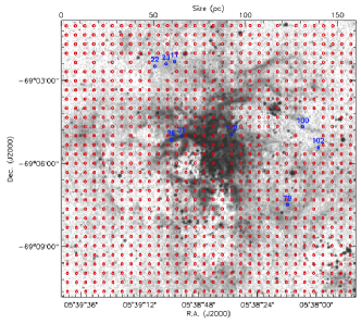
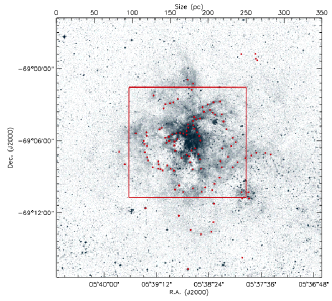
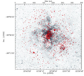
Figure 1: Top panel: GIRAFFE/MEDUSA regular grid overlaid on an optical Digital Sky Survey image of 30 Dor. The spatial separation between each fiber corresponds to 20″($\sim$5 pc). Middle panel: MEDUSA irregular grid. Bottom panel: MEDUSA stellar grid (VFTS survey). The field-of-view on the sky shown in the lower two panels is larger than in the top panel to show all the fibers available. The red rectangle in the middle panel indicates the region covered by the regular grid.

These studies have each provided useful insights about the kinematics of 30 Dor, but the origin of superbubbles and the supersonic velocity dispersions in GHRs are still open questions. In fact, Melnick et al. (1999) suggested that it would be crucial to study the complete 30 Dor nebula at high spatial resolution. Thus, to address these problems, we have obtained high-resolution spectroscopy of 30 Dor, using the FLAMES–Giraffe spectrograph on the Very Large Telescope (VLT) at the Paranal Observatory. Preliminary results from this programme have been published by Torres-Flores et al. (2011).

In this paper we present the data and discuss the general kinematics of 30 Dor, based on analysis of its nebular emission-lines. In future papers we will present analysis of: i) the width of the different emission lines and their contribution to the integrated emission-line profile of 30 Dor; ii) the kinematics of specific regions; iii) the wings detected in the integrated H$\alpha$ profile of 30 Dor; iv) the connection between the kinematics of the ionized warm gas and the X-ray emission in this GHR. This paper is organized as follows. In §2 we present the data and the data-reduction process. In §3 we present the data analysis. In §4 we show the general results obtained with the current data set. Finally, in §5 we summarize our findings.

2 Observations

2.1 Data sets and fiber positioning

To study the detailed kinematics of the ionized gas in 30 Dor we used the MEDUSA fiber mode of the VLT FLAMES–Giraffe spectrograph (Pasquini et al. 2002). Given the proximity of 30 Dor, FLAMES allows us to map, at high spectral and spatial resolution and high signal-to-noise, the main nebular emission lines from the gas, i.e., H$\alpha$ and [Nii] at 6548 and 6584 Å. In this regard, the multiplex of the MEDUSA observing mode enables us to sample a large number of points simultaneously across a relatively wide field-of-view; crucial when studying an extended region like 30 Dor. Given the complex morphology of 30 Dor, three different data sets are used to analyse the its kinematic features: a regular nebular grid, an irregular nebular grid (where the fibers were located in the brightest regions of 30 Dor), and finally a stellar grid. In the following we describe each data set in detail.

Table 1: VLT-FLAMES/MEDUSA observing log for the regular nebular grid.

Field	Coordinates	Setup	N. Fibers	Exp. [s]
1	05:38:42.0, -69:05:40.0	HR14, Medusa1	101	2$\times$600
2	05:38:45.7, -69:05:40.0	HR14, Medusa1	101	2$\times$600
3	05:38:45.7, -69:05:20.0	HR14, Medusa1	76	2$\times$600
4	05:38:42.0, -69:05:20.0	HR14, Medusa1	101	2$\times$600
5	05:38:42.0, -69:05:40.0	HR14, Medusa2	98	2$\times$600
6	05:38:45.7, -69:05:40.0	HR14, Medusa2	98	2$\times$600
7	05:38:45.7, -69:05:20.0	HR14, Medusa2	98	2$\times$600
8	05:38:42.0, -69:05:20.0	HR14, Medusa2	98	2$\times$600
9	05:38:42.0, -69:09:00.0	HR14, Medusa1	71	2$\times$600
10	05:38:42.0, -69:08:40.0	HR14, Medusa1	69	2$\times$600

2.1.1 The regular grid

The observations of the regular nebular grid were carried out on December 3, 2003, using the HR14A Giraffe setting. This provided spectral coverage ranging from 6300 to 6691 Å, with a notional spectral resolving power of $R$ = 17 740 at the central wavelength. We covered a field-of-view of 10^′ $\times$ 10^′ centered on R136. Given that we were limited by the MEDUSA fiber separations, we used three different fiber configurations in offset positions to adequately sample our field-of-view; a total of 10 fields were observed, as summarised in Table LABEL:obslogregular. These fields give a regular grid of 32 $\times$ 30 positions with a spatial sampling of 20^′′, as shown in the top panel of Fig. 1, where the position of each fiber is indicated by a red circle. The aperture of each MEDUSA fiber corresponds to 1.2^′′ on the sky ($\sim$0.3 pc).

Our configurations did not cover some positions given that two MEDUSA fibers were broken, producing some voids in the spatial sampling (see Fig. 1). Out of 960 fiber positions, 49 positions in the grid were not observed. We used nine fibers of the irregular grid to cover some of these missing positions (fibers nos. 11, 22, 23, 28, 31, 79, 100, 102 and 112). The positions of these fibers are indicated by blue numbered circles in the top panel of Fig. 1. In the case of fibers 28 and 31, we calculated an average of the two spectra and replaced this value at the corresponding missing position. The remaining 41 missing positions were filled with the average of the eight closest (and spatially linked) spectra. In this sense, we caution the reader that the spectra visible in the positions of the missing fibers do not represent the real emission at these locations (see Fig. 1).

The centers of the different configurations, setups, and exposure times used to observe 30 Dor are listed in Table LABEL:obslogregular. Given the high surface-brightness displayed by 30 Dor, two sets of observations were taken to avoid saturation effects. In the first instance we took three exposures of 60 s and then we took two exposures of 600 s. At the end, we co-added the two observations of 600 s. The fiber positions for the regular grid are listed in Table A of the Appendix; when a fiber was taken from the irregular grid (as described above), it is labelled as ‘IG’.

Thus, from the regular grid we have obtained 911 equally-spaced spectra across an area of 10’ $\times$ 10’ centered on R136. With that data in-hand, we sorted all the spectra in right ascension and declination. Given that each fiber gave us spectral information for each equally-spaced point, the regular grid enabled us to produce a high-resolution spectroscopic datacube of 30 Dor, spanning 6300 to 6691 Å. This datacube can provide us spatial and spectral information simultaneously, where the spatial information depends on the fiber positions and the spectral information depends on the wavelengths covered by the spectra. For instance, a slice of this datacube centered at H$\alpha$ can give us a monochromatic image of 30 Dor, albeit limited in spatial resolution to 20^′′ by our fiber separation. Despite this fact, the datacube give us an excellent means by which to investigate the kinematics of the large expanding structures in 30 Dor. To illustrate the spectral coverage and primary nebular emission features in the spectra, the integrated spectrum (summed from all spectra in the datacube) is shown in Fig. 2. Given that the most intense emission lines in Fig. 2 correspond to H$\alpha$ and [Nii] $\lambda$6584, we have derived two sub-datacubes centered in these lines, where these sub-cubes cover a range of 500 km s^-1 in velocity.

Figure 2: Integrated nebular spectrum of 30 Dor obtained from summing all of the spectra from the regular grid. The most intense emission line is H$\alpha$, but the intensity axis in the plot is truncated to show the low-intensity emission lines.

In this paper we focus on analysis of the regular grid, but we now briefly introduce the other two data sets as they will be employed in the future studies.

2.1.2 The irregular grid

Additional observations were obtained in the same observing run as the regular grid. This ‘irregular grid’ of MEDUSA positions was selected to observe the brightest nebular regions of 30 Dor, which can be associated with photodissociation regions which lie between the bright nebular and molecular phases. The same high-resolution setup (i.e. HR14A) was used as the regular grid. To reach a high signal-to-noise ratio, nine exposures (each of 600 s) were obtained with this configuration; the positions are shown in the middle panel of Fig. 1 (red circles). The red rectangle indicates the field-of-view covered by the regular nebular grid; as can be seen most of the fibers were located across the filamentary structure of 30 Dor. Each fibre position is listed in Table 2 of the Appendix.

2.1.3 The stellar grid

The observations of the stellar grid were obtained as part of the VFTS (Evans et al. 2011). This multi-epoch spectral survey aims to detect massive binary systems and determine their nature and evolution. The VFTS also aims to study the properties of stellar winds and rotational mixing in O-type stars. To carry out these studies, the survey has observed 800 massive stars, as shown in the bottom panel of Fig. 1. Of relevance here, the red-optical VFTS data were observed with the HR15N Giraffe setup, which has a spectral coverage ranging from 6442 to 6817 Å, at a spectral resolving power of $R$ $=$ 16 000. The HR15N setup provides the additional nebular diagnostic of the [Sii] lines at $\lambda\lambda$6716, 6731 Å, which are not covered by the HR14A observations. Given the large spatial coverage of the VFTS survey, these data can provide additional insights in the study of the kinematics of 30 Dor.

2.2 Data reduction

Reduction of the 2003 data was performed with the ESO pipeline GASGANO and EsoRex software. We observed three bias and flats, which were combined to correct our observations. The wavelength calibration was performed by using the ThAr calibration lamp, from which the instrumental resolution was measured to have a FWHM of 0.4 Å, which corresponds to $R$ $=$ 16 400 at H$\alpha$. All the spectra were corrected to the heliocentric rest frame.

We have compared our processed data with the data available in the Giraffe archive. By visual inspection, the two reductions are in good agreement. Cosmic rays were removed using the task crreject in iraf. Once the data were bias/flat-field corrected and wavelength calibrated, we removed the continuum emission present in the spectra by fitting a polynomial (using the iraf continuum task). In a few cases in the regular grid, the fibers lie close to some stars; for these we use a high-order polynomial to remove the continuum emission. To remove the sky emission lines, we fit Gaussians to one of the lowest intensity spectra. This allowed us to create a template of sky lines, which were removed from all the spectra.

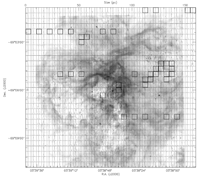
Figure 3: ESO/La Silla H$\alpha$ image of 30 Dor (taken with the EMMI instrument), on which we have over-plotted the H$\alpha$ profile from each fiber of the regular nebular grid. Each small box is 20^′′ $\times$ 20^′′ (5 pc $\times$ 5 pc), with the fibers located at the center of each box. Thick boxes indicate the positions for which we have interpolated the spectra (see §2.1.1).

3 Analysis

Past efforts to understand the internal kinematics of H ii regions have employed profile widths of their emission lines as a diagnostic (e.g., Chu & Kennicutt 1994). Following a similar approach, we use the H$\alpha$ line from our observations to characterize the kinematics of the gas, as it presents the highest signal-to-noise ratio and can be easily resolved into different components in our data. To obtain the line widths we fitted Gaussians automatically to each observed H$\alpha$ profile. In several cases a single Gaussian does not represent the real shape of the multiple profiles that can be seen in this star-forming region (e.g., Melnick et al. 1999). However, this exercise provides some insight about the general behaviour of the H$\alpha$ emission.

We used the mpfit package in idl (Markwardt 2009) to obtain the center, peak intensity and the observed width ($\sigma_{obs}$, uncorrected by instrumental and thermal broadening) of each emission line. Thereafter, where relevant, we fitted multiple Gaussians to the observed profiles using the pan package, which enabled us to select the number of components for each observed profile. This kind of analysis is necessary given the complexity of the emission lines in 30 Dor. For example, Melnick et al. (1999) showed that more than three Gaussian components are needed to reproduce some of the observed profiles. We note that this kind of exercise is (to some degree) arbitrary, given that in several cases we can not resolve two superposed H$\alpha$ profiles (which lie at the same radial velocity, for example), which we would fit with just one Gaussian.

The width of the observed H$\alpha$ profiles take into account the instrumental ($\sigma_{in}$) and thermal ($\sigma_{th}$) widths. The former value depends on the resolution of the instrument, while the latter depends on the thermal motions of the Hydrogen. To obtain a corrected value for the width of the H$\alpha$ emission line, we have subtracted $\sigma_{in}$ and $\sigma_{th}$ from $\sigma_{obs}$ as follows: $\sigma^{2}=\sigma_{obs}^{2}-\sigma_{in}^{2}-\sigma_{th}^{2}$, where $\sigma$ represents the true width of the H$\alpha$ line. As discussed in §2.2, $\sigma_{in}$ was derived from the calibration lamp exposures and has a value of $\sigma_{in}$ $=$ 7.8 km s^-1. For $\sigma_{th}$ we assume hydrogen gas at an electronic temperature of 10⁴ K, from which $\sigma_{th}$ $\sim$ 9.1 km s^-1.

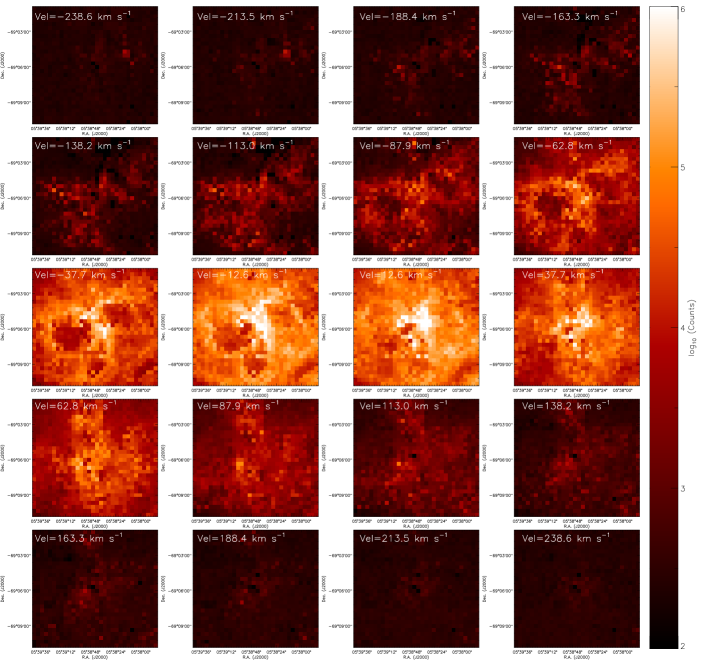
Figure 4: Velocity-sliced view of the 30 Dor datacube centered on the H$\alpha$ line. The velocity with respect to the center of the H$\alpha$ line is shown in the upper left-hand corner of each panel (negative and positive velocities imply radially approaching and receding velocities, respectively). In this figure, a logarithmic scale is used for the intensity of each map.

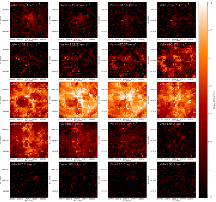
Figure 5: Velocity-sliced view of the 30 Dor datacube centered on the [Nii] $\lambda$6584 line. The velocity with respect to the center of the [Nii] $\lambda$6584 line is shown in the upper left-hand corner of each panel (negative and positive velocities imply radially approaching and receding velocities, respectively). In this figure, a logarithmic scale is used for the intensity of each map.

4 Results

4.1 General view of the 30 Dor spectroscopic datacube

To visualize the complex morphology of the ionized emission in 30 Dor, in Fig. 3 we have plotted the H$\alpha$ profile of each fiber from the regular grid (normalized by the peak of the intensity in each case) over an H$\alpha$ image obtained with the EMMI instrument at the La Silla Observatory.

In Fig. 3 it is possible to correlate the high-resolution spectral information with features seen in the image. The H$\alpha$ profiles in many instances are extremely complex. For example, in the cavity located 1^′ to the east of R136, the H$\alpha$ profiles clearly display multiple components. In fact, the fiber located at the position $\alpha$ $=$ 05^h38^m53.21^s $\delta$ $=$ $-$69^∘05^′59.89^′′ (J2000) displays at least five components (see the last panel of Fig. 7). In general, most of the multiple H$\alpha$ profiles are located in the regions where expanding shells have been previously identified (see Chu & Kennicutt 1994). On the other hand, Fig.  3 shows that the most intense H$\alpha$ emitting regions in 30 Dor (based on its EMMI image) display simple and narrow profiles. In several cases, these bright regions are associated with photodissociation regions (PDRs), which can halt some expanding structures, producing simple profiles. In addition, Fig. 3 shows that some low-intensity regions display simple profiles (for example, in the north-east region), which suggests that no expanding structures lie at that location. By inspecting Fig. 3 it is also possible to identify low-/high-velocity components. For instance, at $\alpha$ $=$ 05^h37^m49.66^s $\delta$ $=$ $-$69^∘02^′39.91^′′ we find a low-intensity component having an approaching velocity larger than 200 km s^-1 compared to the systemic value.

Given the kinematic richness of 30 Dor, we have derived a velocity-sliced view of the datacube, centered on the H$\alpha$ and [Nii] $\lambda$6584 lines. In Fig. 4 we show 20 frames of the datacube. The systemic (zero) velocity was defined by the Gaussian fit to the integrated H$\alpha$ line (i.e. from Fig. 2), in which the line-center was 6568.65 Å, equivalent to $v_{\rm r}$ $=$ 267.4 km s^-1 (where the rest wavelength of the H$\alpha$ emission line was taken from Hirata & Horaguchi 1995) and the velocity interval between each frame was 25.1 km s^-1. In this case, negative and positive velocities imply radially approaching and receding velocities, respectively.

By inspecting the first four frames of Fig. 4, we can see several high-velocity components with respect to the mean velocity of 30 Dor, especially in the neighborhood of the Hodge 301 cluster (the high velocity components in the first and second frames). These components reach approaching velocities larger than 230 km s^-1. By inspecting the datacube we found several low-intensity components that present velocities even larger than 250 km s^-1. For instance, Redman et al. (2003) found several discrete high-speeds knots in 30 Dor, which have velocities of $\pm$200 km s^-1. In the last frames of Fig. 4 we also note several high-velocity components – some of these can be associated with the expanding structure #5 from Chu & Kennicutt (1994, their Fig 1.c).

Another interesting feature that appears in Fig. 4 is the detection of shell-like structures which are visible across all the observed field of 30 Dor (see section §4.4). These structures appear as small voids that increase in size as we move from the blue to the red side of the H$\alpha$ line. It is interesting to note that bluewards of the systemic H$\alpha$ emission the shells are clearly defined, while they are not seen in the frames redwards of the central velocity. Internal extinction produced by dust can produce this signature. Also, molecular clouds located at these positions could hide the red side of the H$\alpha$ emission.

In Fig. 5, we show a similar velocity-sliced view, but now centered on the [Nii] $\lambda$6584 emission line. As in the previous case, the systemic (zero) velocity was derived from the Gaussian fit to the integrated [Nii] $\lambda$6584 line, which gives a radial velocity of $v_{\rm r}$ $=$ 266.1 km s^-1 (6589.29 Å). As to be expected from the reduced intensity of the [Nii] line compared to H$\alpha$, most of the emission is detected at lower expanding velocities than seen in the H$\alpha$ map. While there is a clear correlation between the morphology of the shell-like structures detected in both lines, inspection of Fig. 4 and Fig. 5 shows that several H$\alpha$ and [Nii] $\lambda$6584 high-velocity components do not correlate spatially, which suggests that different physical processes are exciting the gas at these locations. For example, in Fig. 6 we show a high-velocity component in the [Nii] $\lambda$6584 line (black solid line) which presents a strong intensity with respect to their H$\alpha$ counterpart ($\alpha$ $=$ 05^h38^m41.97^s $\delta$ $=$ $-$69^∘04^′40.04^′′). In the same figure, we see the spectrum of the next observed fiber (red dashed line), which present a high-velocity component in H$\alpha$ but with no [Nii] $\lambda$6584 emission ($\alpha$ $=$ 05^h38^m41.96^s $\delta$ $=$ $-$69^∘05^′00.03^′′). We note that in this comparison we are using two adjacent observed fibers. These points all help to illustrate the capabilities of these data in disentangling the complex structures of 30 Dor.

4.2 Complexity of the H$\alpha$ profiles in 30 Doradus

4.2.1 From single to multiple profiles

The wide variety of H$\alpha$ profiles in the data are illustrated by the examples in Fig. 7, which show the four narrowest and broadest profiles (upper and lower panels, respectively). All these profiles correspond to those observed and not to the averaged profiles described in § 2.1.1. A single Gaussian was fitted to each observed profile (as described in § 3), with the coordinates of the fiber position and $\sigma_{obs}$ derived from the fitting process shown in the upper right of each panel. In this analysis, the center of the Gaussian fit gives the overall systemic radial velocity at the position of the fiber, while the width of this fit gives the velocity dispersion of the ionized gas, which must be corrected by the instrumental and thermal widths.

The narrowest H$\alpha$ profile has a $\sigma_{obs}$ $=$ 14.3 km s^-1 (upper left-hand panel in Fig. 7), which corresponds to $\sigma$ $=$ 7.8 km s^-1 once corrected for $\sigma_{th}$ and $\sigma_{in}$. This profile is located in the south-west of the nebula, which is ionized by the LH99 stellar association (Lucke & Hodge 1970) and is also the location of the SN remnant 30 Dor B (Danziger et al. 1981). Two low-intensity components can also be seen in the profile, and these could be associated with an expanding structure. Nonetheless, the main structure of this profile is symmetric and can be well-fitted by a single Gaussian (red dashed line in Fig. 7). The other three narrow H$\alpha$ profiles shown in Fig. 7 display a few low-intensity components, but the main part of the profiles are also well-fitted by a single Gaussian.

In contrast, the broad profiles shown in Fig. 7 clearly display multiple strong components. As expected, these profiles can not be fit by a single Gaussian and their measured widths are the result of a coarse fit that takes into account all the components. All of these broad, multiple profiles lie in shell-like structures. It is interesting to note that the third broad profile shown in Fig. 7 lies just 20^′′ (equivalent to $\sim$5 pc) from the narrow profile located at $\alpha$ $=$ 05^h38^m56.945^s $\delta$ $=$ $-$69^∘06^′19.940^′′. This shows the extremely complex structure of 30 Dor even at small spatial scales.

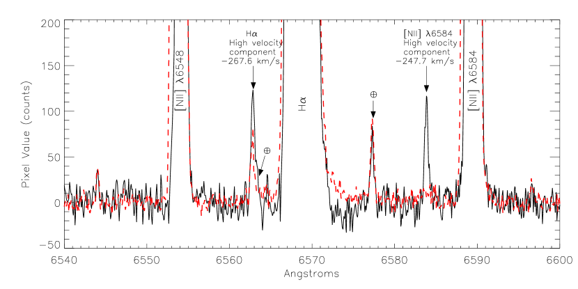
Figure 6: An example of a high-velocity component seen in the [Nii] $\lambda$6584 line. The black solid and red dashed lines correspond to the spectra of two contiguous fibers on the sky. The black solid spectrum shows a [Nii] high velocity component which is intense in comparison with its H$\alpha$ counterpart. This effect is not detected in the red dashed spectrum.

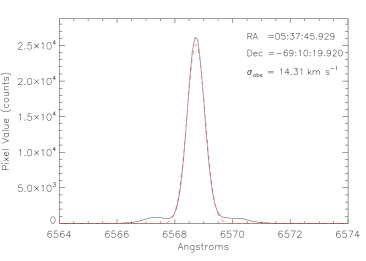
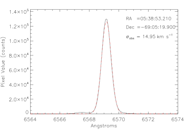
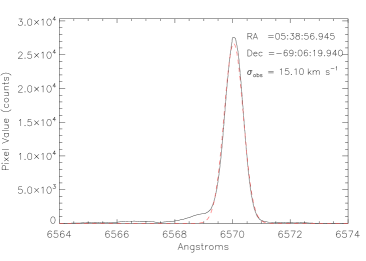
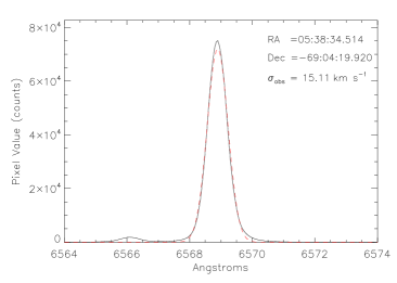
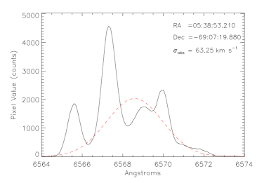
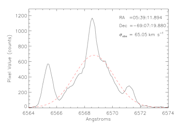
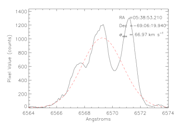
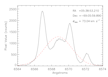
Figure 7: Examples of the different H$\alpha$ morphologies detected in 30 Dor. In the first four panels we show the narrowest H$\alpha$ profiles found in this study. In contrast, the last four panels show the broadest velocities arising from single-profile fits (which are clearly a consequence of multiple components in the observed lines). In each panel we note the coordinates of the observation and $\sigma_{\rm obs}$ of the single-profile Gaussian fit (indicated by the overplotted red dashed lines).

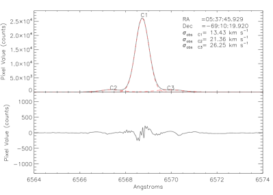
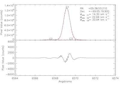
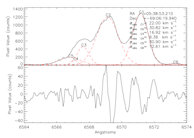
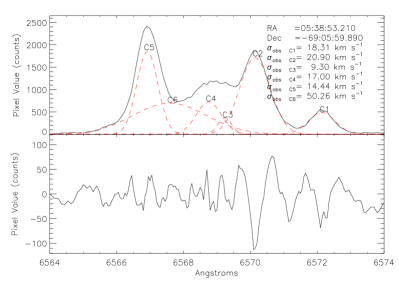
Figure 8: Multiple Gaussian fits to the H$\alpha$ profiles in 30 Dor with the narrowest and broadest single-component velocity dispersions (upper and lower panels, respectively). The black (solid) and red (dashed) lines represent the observed and fitted profiles, respectively; each component is numbered. Residuals of the fits are shown below each fit, which are relatively minor when compared with the intensity of the profiles. In each panel we list the position of the spectra and the $\sigma$ of the different fitted components.

4.2.2 Multiple Gaussian fits: A few examples

To determine the line-broadening mechanism in 30 Dor, Melnick et al. (1999) fitted multiple Gaussian components to the observed H$\alpha$ profiles of different regions. They found that a broad, low-intensity component was necessary to reproduce the wings of all the observed H$\alpha$ profiles. As noted earlier, we have performed multiple Gaussian fits to a subset of profiles using the pan package. In particular, we have examined the two narrowest and broadest H$\alpha$ profiles from single-component fits on the FLAMES data (see Fig. 7), with results of these fits shown in Fig. 8. In each panel of the figure the red (dashed) lines indicate the different Gaussian components used in the fits; the coordinates of the fiber position and the $\sigma_{obs}$ of each fitted component are given in the upper right of the panels. In Fig. 8 we also plot the residuals of the fits, i.e. the difference between the fitted and the observed profile, in which the intensity axis was limited to $\pm$5% of the peak of the observed profile.

For the narrowest H$\alpha$ profile in the data (upper left in Fig. 8), we have fitted three Gaussian components. The two low-intensity components detected at this position present widths smaller than $\sigma_{obs}$ $\sim$ 26 km $s^{-1}$. The strongest component at this position has a corrected width of $\sigma$ $=$ 6.1 km s^-1, i.e., lower than the value obtained by fitting just one Gaussian ($\sigma$ $=$ 7.8 km s^-1, from Fig. 7). By inspecting the residual of these fits, no low-intensity broad component is necessary to explain the observed profile (the residuals are negligible compared with the observed emission). This is of wider interest as this H$\alpha$ profile is located in 30 Dor B, associated with a SN remnant (where we can expect a complex kinematic). In the case of the second-narrowest profile, we have fitted three Gaussian components. The central, most intense feature is fit with a narrow component with a corrected width of 7.8 km s^-1, together with two broader, low-intensity components with corrected widths of 19.2 km s^-1 and 31.8 km s^-1.

The scenario is quite different when multiple Gaussians are fitted to the broadest and more complex H$\alpha$ profiles. In the lower left-hand panel of Fig. 8, we show that at least six components are necessary to reproduce the observed emission line at that position. The broadest component has a corrected width of $\sigma$ $=$ 28.5 km s^-1. As in the previous cases, the residual is negligible compared with the intensity of the profiles. Finally, in the lower right-hand panel of Fig. 8 we show another spectrum which requires six components to fit the observations. In this case, the broadest component has a corrected width of $\sigma$ $=$ 48.8 km s^-1. It is interesting to note that four of the six broad components used in the Gaussian fits shown in the lower panel of Fig. 8 display supersonic widths (once corrected by $\sigma_{th}$ and $\sigma_{ins}$). Despite other Gaussian components can be fitted in these wide profiles, our results suggest the presence of a highly turbulent gas at these locations.

We note that Melnick et al. (1999) found that most of the H$\alpha$ profiles in their analysis required the presence of a low-intensity broad component with $\sigma$ $=$ 45 km s^-1, Moreover, this broad component was required to fit their integrated H$\alpha$ profile of 30 Dor, centered at the radial velocity of this GHR. This component was not identified in the two narrowest profiles observed by FLAMES, nor in the second broadest profile (shown in Fig. 8). In fact, the broad components that we have identified are not at the systemic radial velocity of the 30 Dor gas; the origin of the broad component in 30 Dor, if real, is still a mystery.

Figure 9: Single and two-component Gaussian fits to the integrated H$\alpha$ profile (upper and lower panels, respectively). The fitted components are shown by the red (dashed) lines and their widths are indicated in the upper right of each panel.

4.2.3 The integrated H$\alpha$ profile of 30 Doradus

Fits to the integrated H$\alpha$ profile (from Fig. 2) are shown in Fig. 9. For a single-component fit we found a corrected width of $\sigma$ $=$ 26.5 km s^-1 ($\sigma_{\rm obs}$ $=$ 29.1 km s^-1). Note from the figure that the blue and red wings of the integrated profile can not be fitted by one component – a second, broader component is required, as shown in the lower panel of Fig. 9. By using narrow, high-intensity and broad, low-intensity components, we obtain a much better fit to the observed H$\alpha$ profile of 30 Dor. In this case, the narrow and the broad components have corrected widths of $\sigma$ $=$ 21.2 km s^-1 ($\sigma_{\rm obs}$ $=$ 24.4 km s^-1) and $\sigma$ $=$ 47.6 km s^-1 ($\sigma_{\rm obs}$ $=$ 49.1 km s^-1), respectively. Our result for the narrow component is in good agreement with the corrected width from Melnick et al. (1999, $\sigma$ $=$ 22 km s^-1) from the data of Chu & Kennicutt (1994); our broader component is marginally wider than the $\sigma$ $=$ 44 km s^-1 from Melnick et al. By comparing the bottom panel of Fig. 9 with the Fig. 4 from Melnick et al., we note that our broad component is less intense (with respect to the height of the profile) than their broad fit, perhaps due to the different spatial extents that the two studies cover.

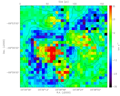
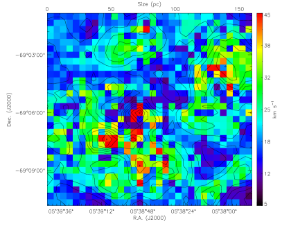
Figure 10: Radial line-of-sight systemic velocity map (upper panel) and velocity dispersion map (lower panel) of 30 Doradus from analysis of the H$\alpha$ emission in the FLAMES spectra. North at the top and east to the left. The radial velocity map was corrected by the systemic velocity of 30 Dor.

4.3 The velocity map of 30 Doradus

As discussed in § 3, we have fitted a single-component Gaussian to each H$\alpha$ profile. We have used the center and $\sigma$ (corrected by $\sigma_{in}$ and $\sigma_{th}$) of each fit to derive the radial line-of-sight systemic velocity field and the velocity dispersion map of 30 Dor, as shown in Fig. 10. In the case of the radial velocity field, it was corrected by the systemic velocity of 30 Dor. Although a single Gaussian fit does not represent the exact radial velocity of regions that display multiple profiles, these fits still give us important information regarding the complexity of the observed profiles. i.e., regions that present multiple profiles will have large values of $\sigma$ (as shown in Fig. 7). In this sense, both maps help us to understand the overall dynamics of 30 Dor.

In the top panel of Fig. 10 we show the velocity field, centered on its integrated H$\alpha$ line (see Fig. 9). Approaching and receding regions are represented by blue and red colors, respectively. Green regions are at the systemic velocity of the gas in 30 Dor. In order to show the whole kinematic behaviour of 30 Doradus, we chose a dynamic range of 70 km s^-1 in the velocity map. As shown in the velocity map, the north-eastern and south-western regions remain at roughly the systemic velocity (258.3 km s^-1, see § 4.1). In the case of the south-western region, the velocity dispersion map (lower panel of Fig. 10) shows several narrow H$\alpha$ profiles, especially in the neighbourhood of 30 Dor B (in which we find the narrowest H$\alpha$ profile detected in the FLAMES spectra).

Another remarkable feature to note from Fig. 10 is the presence of large expanding structures. The north-eastern edge of shell #2 (see Chu & Kennicutt 1994) appears to have negative velocities (with respect to the systemic velocity) while the cavity of this structure appears to have positive velocities, giving a 3D view of this shell. Several profiles within this cavity display large values for $\sigma_{obs}$, which are the result of fitting a single Gaussian over at least two H$\alpha$ components. In general, Fig. 10 shows that the outer regions of 30 Dor are at the same velocity of the integrated profile of all the spectra, and also that the outer regions can typically be fitted by a single Gaussian component.

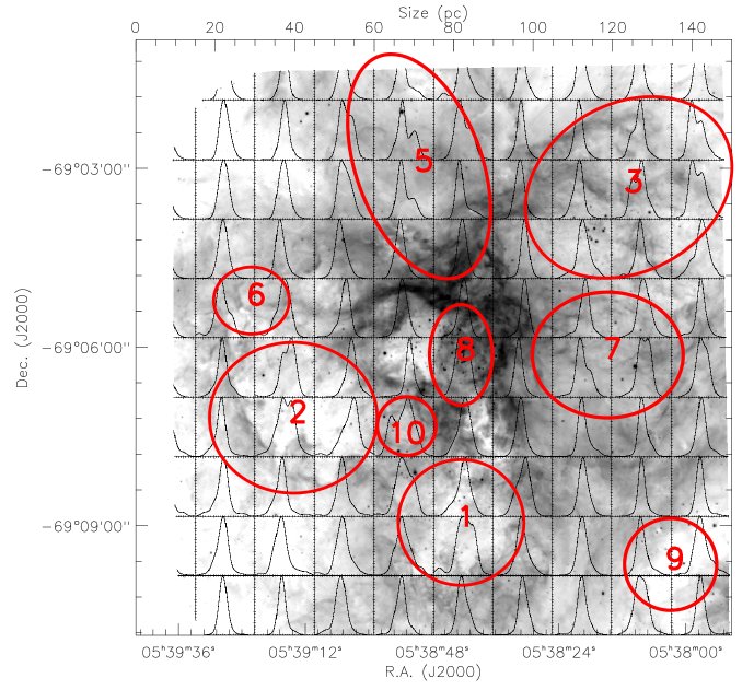
Figure 11: Top panel: Large expanding structures previously catalogued in 30 Dor (nos. 1, 2, 3 and 5) with the five new expanding structures (nos. 6, 7, 8, 9 and 10) identified here. Bottom Panel: $\chi^{2}$ map for the H$\alpha$ cube of 30 Dor, derived from a single Gaussian fit on each observed profile.

4.4 Large expanding structures in 30 Doradus

We have used the H$\alpha$ datacube to search for large expanding structures. These structures are characterized by double components in their emission-line profiles, signature of expanding ionized gas at these positions. To identify these structures, we have applied two methods. In a first instance, we have integrated the H$\alpha$ profiles shown in Fig. 3 over regions of 1^′ $\times$ 1^′, given the poor spatial sampling of our data. Then, these integrated profiles were visually inspected in order to search for double components. In Fig. 11, we superimpose these integrated H$\alpha$ profiles over the H$\alpha$ image. At least ten large expanding structures can be identified and are overlaid on the image in Fig. 11. Some of these – shells 1, 2, 3, and 5 – were catalogued previously (Cox & Deharveng, 1983; Wang & Helfand, 1991), so we adopt the same numbers. Structures 6, 7, 8, 9 and 10 are identified for the first time by this work. These expanding regions present double components in their H$\alpha$ emission, as can be noted from Fig. 11.

In a second instance, the large expanding structures were searched by using the Gaussian fit on each individual profile. Given that simple H$\alpha$ profiles can be fitted with a single Gaussian, the $\chi^{2}$ value for these fits will be lower than the value presented by H$\alpha$ profiles that display double or multiple components. This fact can indicate the location of expanding structures, as profiles that are not well fitted by a single Gaussian. In this sense, we have derived a map with the $\chi^{2}$ values obtained from a single Gaussian fit to the H$\alpha$ datacube of 30 Dor, which is shown in the bottom panel of Fig. 11. In this case, the Gaussian fit was performed on each observed H$\alpha$ profile, which was normalized by the total intensity of each profile. Inspecting the bottom panel of Fig. 11, we detect several structures that can not be fitted with a single Gaussian and that could be associated with expanding regions. Interestingly, most of these structures lie on the same position of the expanding regions detected by visual inspection. This correlation is clear for regions #6 and #8. Between regions #1, #2 and #8, the $\chi^{2}$ map shows another peak in the $\chi^{2}$values. Inspection of the profiles at that location (top panel of Fig. 11) suggest the presence of a small expanding structure. Despite the analysis of the $\chi^{2}$ map is clearly more quantitative than the visual inspection of the H$\alpha$ profiles, it results necessary to combine both information in order to determine the size and the real nature of the expanding structures.

Of particular interest is structure #6. At this position we do not find any star that could be producing an expansion of the ionized gas. Studies of the diffuse X-ray emission seen by the Chandra X-ray Observatory appear to indicate a single-temperature thermal plasma in this region, but with spectral signatures of both collisional ionization equilibrium and non-equilibrium ionization (Townsley et al. in preparation). This may indicate a plasma that has undergone a recent shock and is transitioning back to ionization equilibrium, possibly consistent with a SN remnant. This scenario is compatible with the expanding structure found in this work; we will analyse the main properties of these newly-detected expanding bubbles in a future study.

Another method to search for expanding structures in GHRs is via analysis of long-slit observations, e.g. the analysis in 30 Dor by Chu & Kennicutt (1994). To mimic their long-slit observations, we have produced 2D cuts along selected rows of the FLAMES datacube (i. e. at different declinations). In Fig. 12 we show these 2D cuts of rows 10, 11, 12, 13 and 14 of the datacube, respectively (see Table A for the RA and Dec of these positions). Row #10 passes across the southern region of the expanding structure #2 (see Fig. 11), while rows #11, #12, #13 and #14 go northwards across the structure #2. In these spectra, we can clearly see the H$\alpha$ and [Nii] $\lambda\lambda$6548, 6584 lines, with H$\alpha$ the brightest feature. By inspecting the H$\alpha$ emission in rows 11-14 from Fig. 12, we can note the presence of an expanding structure (as indicated by the black arrows). This structure, which can be identified with shell #2 in Fig. 11, appears as a semi-arc of emission close to the center of the H$\alpha$ line (see the red-dashed ellipse, in the case of row #14). The expansion of this structure can be clearly identified on the blueward side of the H$\alpha$ line (see black arrows), but it is not easily seen on the redward side. This structure may be off-center with respect to the systemic H$\alpha$ emission of 30 Dor.

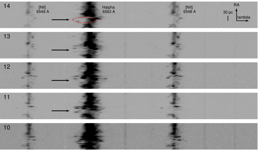
Figure 12: 2D cut obtained from the spectroscopic datacube of 30 Doradus. These spectra correspond to rows 10, 11, 12, 13 and 14 from bottom to top (the numbers are indicated in the top left corner of each panel). The brightest lines correspond (from left-to-right) to [Nii] $\lambda$6548, H$\alpha$ and [Nii] $\lambda$6584. The black arrows indicate the position of an expanding structure. As an example, the red-dashed ellipse indicates the location of this expanding structure in row #14.

5 Summary and conclusions

We have presented new VLT-FLAMES spectroscopy obtained to study the kinematics of the ionized gas in 30 Doradus. These data consist of regular and irregular grids of nebular observations, combined with a stellar grid. The regular grid was combined into a datacube, allowing us to analyse the primary kinematic features of 30 Dor, with the main points now briefly summarised.

1. The kinematics of the ionized gas in 30 Dor are complex, with a diverse range of single and multiple H$\alpha$ profiles. In the brightest regions the H$\alpha$ profiles are found to be simple and narrow. However, the narrowest H$\alpha$ profile observed in the data lies close to 30 Dor B, where a past SN explosion occurred. This is surprising in the sense that 30 Dor B might be expected to be dominated by the kinematics of the SN remnant (i.e., multiple emission profiles and high-velocity components).

2. We have applied multi-Gaussian fits to the H$\alpha$ profiles of the two narrowest and broadest single-component fits detected in 30 Dor. We do not detect the presence of a broad, low-intensity component, as reported by Melnick et al. (1999) for all of their observed H$\alpha$ profiles.

3. However, the integrated H$\alpha$ profile of 30 Dor does display broad wings, and required Gaussian fits that include both narrow and broad components (as per Melnick et al.).

4. We have derived the velocity field and a velocity dispersion map of 30 Dor. By inspecting these maps, we found that the outer parts of our observed regular grid (i.e. a field-of-view of 10^′ $\times$ 10^′ centered on R136) are at the same velocity of the integrated H$\alpha$ profile of 30 Dor.

5. Using the spectroscopic datacube of 30 Dor, we have identified at least five previously unclassified expanding structures. In one case (structure #6), we did not find any star associated with the expanding gas at that location.

Areas for future work include a detailed analysis of the supersonic velocity in the integrated profile of 30 Dor (besides the origin of the wings in this profile) and a more in-depth study of the individual kinematic structures identified and discussed here.

Appendix A Position of the fibers

In Table A.1 we list the fiber positioning of the regular nebular grid (which does not include the positions of the broken fibers). In the cases where we used a fiber from the irregular nebular grid to complete our regular grid, we label that fiber as ‘IG’ (irregular grid). In Table A.2 we list the fiber positions of the irregular nebular grid.

Table 2: Fiber positions of the regular nebular grid.

ID	X	Y	RA (J2000)	DEC (J2000)	Data
	pix	pix	h:m:s	d:m:s
1	1	1	05:39:41.801	-69:10:39.900	Obs.
2	2	1	05:39:38.059	-69:10:39.900	Obs.
3	3	1	05:39:34.320	-69:10:39.900	Obs.
4	4	1	05:39:30.590	-69:10:39.900	Obs.
5	5	1	05:39:26.849	-69:10:39.900	Obs.
6	6	1	05:39:23.110	-69:10:39.900	Obs.
7	7	1	05:39:19.370	-69:10:39.900	Obs.
8	8	1	05:39:15.629	-69:10:39.900	Obs.
9	9	1	05:39:11.899	-69:10:39.900	Obs.
10	10	1	05:39:08.160	-69:10:39.900	Obs.
11	11	1	05:39:04.421	-69:10:39.900	Obs.
12	12	1	05:39:00.679	-69:10:39.900	Obs.
13	13	1	05:38:56.950	-69:10:39.900	Obs.
14	14	1	05:38:53.210	-69:10:39.900	Obs.
15	15	1	05:38:49.469	-69:10:39.900	Obs.
16	16	1	05:38:45.730	-69:10:39.900	Obs.
17	17	1	05:38:42.000	-69:10:39.900	Obs.
18	18	1	05:38:38.261	-69:10:39.900	Obs.
19	19	1	05:38:34.519	-69:10:39.900	Obs.
20	20	1	05:38:30.780	-69:10:39.900	Obs.
21	21	1	05:38:27.050	-69:10:39.900	Obs.
22	22	1	05:38:23.309	-69:10:39.900	Obs.
23	23	1	05:38:19.570	-69:10:39.900	Obs.
24	24	1	05:38:15.830	-69:10:39.900	Obs.
25	25	1	05:38:12.101	-69:10:39.900	Obs.
26	26	1	05:38:08.359	-69:10:39.900	Obs.
27	27	1	05:38:04.620	-69:10:39.900	Obs.
28	28	1	05:38:00.881	-69:10:39.900	Obs.
29	29	1	05:37:57.139	-69:10:39.900	Obs.
30	30	1	05:37:53.410	-69:10:39.900	Obs.
31	31	1	05:37:49.670	-69:10:39.900	Obs.
32	32	1	05:37:45.929	-69:10:39.900	Obs.
33	1	2	05:39:41.801	-69:10:19.920	Obs.
34	2	2	05:39:38.059	-69:10:19.920	Obs.
35	3	2	05:39:34.320	-69:10:19.920	Obs.
36	4	2	05:39:30.590	-69:10:19.920	Obs.
37	5	2	05:39:26.849	-69:10:19.920	Obs.
38	6	2	05:39:23.110	-69:10:19.920	Obs.
39	7	2	05:39:19.370	-69:10:19.920	Obs.
40	8	2	05:39:15.629	-69:10:19.920	Obs.
41	9	2	05:39:11.899	-69:10:19.920	Obs.
42	10	2	05:39:08.160	-69:10:19.920	Obs.
43	11	2	05:39:04.421	-69:10:19.920	Obs.
44	12	2	05:39:00.679	-69:10:19.920	Obs.
45	13	2	05:38:56.950	-69:10:19.920	Obs.
46	14	2	05:38:53.210	-69:10:19.920	Obs.
47	15	2	05:38:49.469	-69:10:19.920	Obs.
48	16	2	05:38:45.730	-69:10:19.920	Obs.
49	17	2	05:38:42.000	-69:10:19.920	Obs.
50	18	2	05:38:38.261	-69:10:19.920	Obs.
51	19	2	05:38:34.519	-69:10:19.920	Obs.
52	20	2	05:38:30.780	-69:10:19.920	Obs.
53	21	2	05:38:27.050	-69:10:19.920	Obs.
54	22	2	05:38:23.309	-69:10:19.920	Obs.
55	23	2	05:38:19.570	-69:10:19.920	Obs.
56	24	2	05:38:15.830	-69:10:19.920	Obs.
57	25	2	05:38:12.101	-69:10:19.920	Obs.
58	26	2	05:38:08.359	-69:10:19.920	Obs.
59	27	2	05:38:04.620	-69:10:19.920	Obs.
60	28	2	05:38:00.881	-69:10:19.920	Obs.
61	29	2	05:37:57.139	-69:10:19.920	Obs.
62	30	2	05:37:53.410	-69:10:19.920	Obs.
63	31	2	05:37:49.670	-69:10:19.920	Obs.
64	32	2	05:37:45.929	-69:10:19.920	Obs.
65	1	3	05:39:41.796	-69:09:59.900	Obs.
66	2	3	05:39:38.059	-69:09:59.900	Obs.
67	3	3	05:39:34.325	-69:09:59.900	Obs.
68	4	3	05:39:30.590	-69:09:59.900	Obs.
69	5	3	05:39:26.846	-69:09:59.900	Obs.
70	6	3	05:39:23.110	-69:09:59.900	Obs.
71	7	3	05:39:19.366	-69:09:59.900	Obs.
72	8	3	05:39:15.629	-69:09:59.900	Obs.
73	9	3	05:39:11.894	-69:09:59.900	Obs.
74	10	3	05:39:08.160	-69:09:59.900	Obs.
75	11	3	05:39:04.416	-69:09:59.900	Obs.
76	12	3	05:39:00.679	-69:09:59.900	Obs.
77	13	3	05:38:56.945	-69:09:59.900	Obs.
78	14	3	05:38:53.210	-69:09:59.900	Obs.
79	15	3	05:38:49.466	-69:09:59.900	Obs.
80	16	3	05:38:45.730	-69:09:59.900	Obs.
81	17	3	05:38:41.995	-69:09:59.900	Obs.
82	18	3	05:38:38.261	-69:09:59.900	Obs.
83	19	3	05:38:34.514	-69:09:59.900	Obs.
84	20	3	05:38:30.780	-69:09:59.900	Obs.
85	21	3	05:38:27.050	-69:09:59.900	Obs.
86	22	3	05:38:23.309	-69:09:59.900	Obs.
87	23	3	05:38:19.565	-69:09:59.900	Obs.
88	24	3	05:38:15.830	-69:09:59.900	Obs.
89	25	3	05:38:12.096	-69:09:59.900	Obs.
90	26	3	05:38:08.359	-69:09:59.900	Obs.
91	27	3	05:38:04.615	-69:09:59.900	Obs.
92	28	3	05:38:00.881	-69:09:59.900	Obs.
93	29	3	05:37:57.146	-69:09:59.900	Obs.
94	30	3	05:37:53.410	-69:09:59.900	Obs.
95	31	3	05:37:49.666	-69:09:59.900	Obs.
96	32	3	05:37:45.929	-69:09:59.900	Obs.
97	1	4	05:39:41.796	-69:09:39.850	Obs.
98	2	4	05:39:38.059	-69:09:39.920	Obs.
99	3	4	05:39:34.325	-69:09:39.920	Obs.
100	4	4	05:39:30.590	-69:09:39.920	Obs.
101	5	4	05:39:26.846	-69:09:39.920	Obs.
102	6	4	05:39:23.110	-69:09:39.920	Obs.
103	7	4	05:39:19.366	-69:09:39.850	Obs.
104	8	4	05:39:15.629	-69:09:39.920	Obs.
105	9	4	05:39:11.894	-69:09:39.850	Obs.
106	10	4	05:39:08.160	-69:09:39.920	Obs.
107	11	4	05:39:04.416	-69:09:39.920	Obs.
108	12	4	05:39:00.679	-69:09:39.920	Obs.
109	13	4	05:38:56.945	-69:09:39.920	Obs.
110	14	4	05:38:53.210	-69:09:39.920	Obs.
111	15	4	05:38:49.466	-69:09:39.920	Obs.
112	16	4	05:38:45.730	-69:09:39.920	Obs.
113	17	4	05:38:41.995	-69:09:39.920	Obs.
114	18	4	05:38:38.261	-69:09:39.920	Obs.
115	19	4	05:38:34.514	-69:09:39.920	Obs.
116	20	4	05:38:30.780	-69:09:39.920	Obs.
117	21	4	05:38:27.050	-69:09:39.920	Obs.
118	22	4	05:38:23.309	-69:09:39.920	Obs.
119	23	4	05:38:19.565	-69:09:39.920	Obs.
120	24	4	05:38:15.830	-69:09:39.920	Obs.
121	25	4	05:38:12.096	-69:09:39.920	Obs.
122	26	4	05:38:08.359	-69:09:39.920	Obs.
123	27	4	05:38:04.615	-69:09:39.920	Obs.
124	28	4	05:38:00.881	-69:09:39.920	Obs.
125	29	4	05:37:57.146	-69:09:39.920	Obs.
126	30	4	05:37:53.410	-69:09:39.920	Obs.
127	31	4	05:37:49.666	-69:09:39.920	Obs.
128	32	4	05:37:45.929	-69:09:39.920	Obs.
129	1	5	05:39:41.796	-69:09:19.910	Obs.
130	2	5	05:39:38.059	-69:09:19.910	Obs.
131	3	5	05:39:34.325	-69:09:19.910	Obs.
132	4	5	05:39:30.590	-69:09:19.910	Obs.
133	5	5	05:39:26.846	-69:09:19.910	Obs.
134	6	5	05:39:23.110	-69:09:19.910	Obs.
135	7	5	05:39:19.366	-69:09:19.910	Obs.
136	8	5	05:39:15.629	-69:09:19.910	Obs.
137	9	5	05:39:11.894	-69:09:19.910	Obs.
138	10	5	05:39:08.160	-69:09:19.910	Obs.
139	11	5	05:39:04.416	-69:09:19.910	Obs.
140	12	5	05:39:00.679	-69:09:19.910	Obs.
141	13	5	05:38:56.945	-69:09:19.910	Obs.
142	14	5	05:38:53.210	-69:09:19.910	Obs.
143	15	5	05:38:49.466	-69:09:19.910	Obs.
144	16	5	05:38:45.730	-69:09:19.910	Obs.
145	17	5	05:38:41.995	-69:09:19.910	Obs.
146	18	5	05:38:38.261	-69:09:19.910	Obs.
147	19	5	05:38:34.514	-69:09:19.910	Obs.
148	20	5	05:38:30.780	-69:09:19.910	Obs.
149	21	5	05:38:27.050	-69:09:19.910	Obs.
150	22	5	05:38:23.309	-69:09:19.910	Obs.
151	23	5	05:38:19.565	-69:09:19.910	Obs.
152	24	5	05:38:15.830	-69:09:19.910	Obs.
153	25	5	05:38:12.096	-69:09:19.910	Obs.
154	26	5	05:38:08.359	-69:09:19.910	Obs.
155	27	5	05:38:04.615	-69:09:19.910	Obs.
156	28	5	05:38:00.881	-69:09:19.910	Obs.
157	29	5	05:37:57.146	-69:09:19.910	Obs.
158	30	5	05:37:53.410	-69:09:19.910	Obs.
159	31	5	05:37:49.666	-69:09:19.910	Obs.
160	32	5	05:37:45.929	-69:09:19.910	Obs.
161	1	6	05:39:41.796	-69:08:59.860	Obs.
162	2	6	05:39:38.059	-69:08:59.930	Obs.
163	3	6	05:39:34.325	-69:08:59.930	Obs.
164	4	6	05:39:30.590	-69:08:59.930	Obs.
165	5	6	05:39:26.846	-69:08:59.930	Obs.
166	6	6	05:39:23.110	-69:08:59.930	Obs.
167	7	6	05:39:19.366	-69:08:59.860	Obs.
168	8	6	05:39:15.629	-69:08:59.930	Obs.
169	9	6	05:39:11.894	-69:08:59.860	Obs.
170	10	6	05:39:08.160	-69:08:59.930	Obs.
171	11	6	05:39:04.416	-69:08:59.930	Obs.
172	12	6	05:39:00.679	-69:08:59.930	Obs.
173	13	6	05:38:56.945	-69:08:59.930	Obs.
174	14	6	05:38:53.210	-69:08:59.930	Obs.
175	15	6	05:38:49.466	-69:08:59.930	Obs.
176	16	6	05:38:45.730	-69:08:59.930	Obs.
177	17	6	05:38:41.995	-69:08:59.930	Obs.
178	18	6	05:38:38.261	-69:08:59.930	Obs.
179	19	6	05:38:34.514	-69:08:59.930	Obs.
180	20	6	05:38:30.780	-69:08:59.930	Obs.
181	21	6	05:38:27.050	-69:08:59.930	Obs.
182	22	6	05:38:23.309	-69:08:59.930	Obs.
183	23	6	05:38:19.565	-69:08:59.930	Obs.
184	24	6	05:38:15.830	-69:08:59.930	Obs.
185	25	6	05:38:12.096	-69:08:59.930	Obs.
186	26	6	05:38:08.359	-69:08:59.930	Obs.
187	27	6	05:38:04.615	-69:08:59.930	Obs.
188	28	6	05:38:00.881	-69:08:59.930	Obs.
189	29	6	05:37:57.146	-69:08:59.930	Obs.
190	30	6	05:37:53.410	-69:08:59.930	Obs.
191	31	6	05:37:49.666	-69:08:59.930	Obs.
192	32	6	05:37:45.929	-69:08:59.930	Obs.
193	1	7	05:39:41.796	-69:08:39.910	Obs.
194	2	7	05:39:38.059	-69:08:39.910	Obs.
195	3	7	05:39:34.325	-69:08:39.910	Obs.
196	4	7	05:39:30.590	-69:08:39.910	Obs.
197	5	7	05:39:26.846	-69:08:39.910	Obs.
198	6	7	05:39:23.110	-69:08:39.910	Obs.
199	7	7	05:39:19.366	-69:08:39.910	Obs.
200	8	7	05:39:15.629	-69:08:39.910	Obs.
201	9	7	05:39:11.894	-69:08:39.910	Obs.
202	10	7	05:39:08.160	-69:08:39.910	Obs.
203	11	7	05:39:04.416	-69:08:39.910	Obs.
204	12	7	05:39:00.679	-69:08:39.910	Obs.
205	13	7	05:38:56.945	-69:08:39.910	Obs.
206	14	7	05:38:53.210	-69:08:39.910	Obs.
207	15	7	05:38:49.466	-69:08:39.910	Obs.
208	16	7	05:38:45.730	-69:08:39.910	Obs.
209	17	7	05:38:41.995	-69:08:39.910	Obs.
210	18	7	05:38:38.261	-69:08:39.910	Obs.
211	19	7	05:38:34.514	-69:08:39.910	Obs.
212	20	7	05:38:30.780	-69:08:39.910	Obs.
213	21	7	05:38:27.046	-69:08:39.910	Obs.
214	22	7	05:38:23.309	-69:08:39.910	Obs.
215	23	7	05:38:19.565	-69:08:39.910	Obs.
216	24	7	05:38:15.830	-69:08:39.910	Obs.
217	25	7	05:38:12.096	-69:08:39.910	Obs.
218	26	7	05:38:08.359	-69:08:39.910	Obs.
219	27	7	05:38:04.615	-69:08:39.910	Obs.
220	28	7	05:38:00.881	-69:08:39.910	Obs.
221	29	7	05:37:57.146	-69:08:39.910	Obs.
222	30	7	05:37:53.410	-69:08:39.910	Obs.
223	31	7	05:37:49.666	-69:08:39.910	Obs.
224	32	7	05:37:45.929	-69:08:39.910	Obs.
225	1	8	05:39:41.796	-69:08:19.860	Obs.
226	2	8	05:39:38.059	-69:08:19.930	Obs.
227	3	8	05:39:34.325	-69:08:19.930	Obs.
228	4	8	05:39:30.590	-69:08:19.930	Obs.
229	5	8	05:39:26.846	-69:08:19.930	Obs.
230	6	8	05:39:23.110	-69:08:19.930	Obs.
231	7	8	05:39:19.366	-69:08:19.860	Obs.
232	8	8	05:39:15.629	-69:08:19.930	Obs.
233	9	8	05:39:11.894	-69:08:19.860	Obs.
234	10	8	05:39:08.160	-69:08:19.930	Obs.
235	11	8	05:39:04.416	-69:08:19.930	Obs.
236	12	8	05:39:00.679	-69:08:19.930	Obs.
237	13	8	05:38:56.945	-69:08:19.930	Obs.
238	14	8	05:38:53.210	-69:08:19.930	Obs.
239	15	8	05:38:49.466	-69:08:19.860	Obs.
240	16	8	05:38:45.730	-69:08:19.930	Obs.
241	17	8	05:38:41.995	-69:08:19.860	Obs.
242	18	8	05:38:38.261	-69:08:19.930	Obs.
243	19	8	05:38:34.514	-69:08:19.860	Obs.
244	20	8	05:38:30.780	-69:08:19.930	Obs.
245	21	8	05:38:27.046	-69:08:19.860	Obs.
246	22	8	05:38:23.309	-69:08:19.930	Obs.
247	23	8	05:38:19.565	-69:08:19.860	Obs.
248	24	8	05:38:15.830	-69:08:19.930	Obs.
249	25	8	05:38:12.096	-69:08:19.860	Obs.
250	26	8	05:38:08.359	-69:08:19.930	Obs.
251	27	8	05:38:04.615	-69:08:19.860	Obs.
252	28	8	05:38:00.881	-69:08:19.930	Obs.
253	29	8	05:37:57.146	-69:08:19.860	Obs.
254	30	8	05:37:53.410	-69:08:19.930	Obs.
255	31	8	05:37:49.666	-69:08:19.860	Obs.
256	32	8	05:37:45.929	-69:08:19.930	Obs.
257	1	9	05:39:41.796	-69:07:59.920	Obs.
258	2	9	05:39:38.059	-69:07:59.920	Obs.
259	3	9	05:39:34.325	-69:07:59.920	Obs.
260	4	9	05:39:30.590	-69:07:59.920	Obs.
261	5	9	05:39:26.846	-69:07:59.920	Obs.
262	6	9	05:39:23.110	-69:07:59.920	Obs.
263	7	9	05:39:19.366	-69:07:59.920	Obs.
264	8	9	05:39:15.629	-69:07:59.920	Obs.
265	9	9	05:39:11.894	-69:07:59.920	Obs.
266	10	9	05:39:08.160	-69:07:59.920	Obs.
267	11	9	05:39:04.416	-69:07:59.920	Obs.
268	12	9	05:39:00.679	-69:07:59.920	Obs.
269	13	9	05:38:56.945	-69:07:59.920	Obs.
270	14	9	05:38:53.210	-69:07:59.920	Obs.
271	15	9	05:38:49.466	-69:07:59.920	Obs.
272	16	9	05:38:45.730	-69:07:59.920	Obs.
273	17	9	05:38:41.995	-69:07:59.920	Obs.
274	18	9	05:38:38.261	-69:07:59.920	Obs.
275	19	9	05:38:34.514	-69:07:59.920	Obs.
276	20	9	05:38:30.780	-69:07:59.920	Obs.
277	21	9	05:38:27.046	-69:07:59.920	Obs.
278	22	9	05:38:23.309	-69:07:59.920	Obs.
279	23	9	05:38:19.565	-69:07:59.920	Obs.
280	24	9	05:38:15.830	-69:07:59.920	Obs.
281	25	9	05:38:12.096	-69:07:59.920	Obs.
282	26	9	05:38:08.359	-69:07:59.920	Obs.
283	27	9	05:38:04.615	-69:07:59.920	Obs.
284	28	9	05:38:00.881	-69:07:59.920	Obs.
285	29	9	05:37:57.146	-69:07:59.920	Obs.
286	30	9	05:37:53.410	-69:07:59.920	Obs.
287	31	9	05:37:49.666	-69:07:59.920	Obs.
288	32	9	05:37:45.929	-69:07:59.920	Obs.
289	1	10	05:39:41.796	-69:07:39.860	Obs.
290	2	10	05:39:38.059	-69:07:39.940	Obs.
291	3	10	05:39:34.325	-69:07:39.940	Obs.
292	4	10	05:39:30.590	-69:07:39.940	Obs.
293	5	10	05:39:26.846	-69:07:39.940	Obs.
294	6	10	05:39:23.110	-69:07:39.940	Obs.
295	7	10	05:39:19.366	-69:07:39.860	Obs.
296	8	10	05:39:15.629	-69:07:39.940	Obs.
297	9	10	05:39:11.894	-69:07:39.860	Obs.
298	10	10	05:39:08.160	-69:07:39.940	Obs.
299	11	10	05:39:04.416	-69:07:39.940	Obs.
300	12	10	05:39:00.679	-69:07:39.940	Obs.
301	13	10	05:38:56.945	-69:07:39.940	Obs.
302	14	10	05:38:53.210	-69:07:39.940	Obs.
303	15	10	05:38:49.466	-69:07:39.860	Obs.
304	16	10	05:38:45.730	-69:07:39.940	Obs.
305	17	10	05:38:41.995	-69:07:39.860	Obs.
306	18	10	05:38:38.261	-69:07:39.940	Obs.
307	19	10	05:38:34.512	-69:07:40.080	No Obs.
308	20	10	05:38:30.780	-69:07:39.940	Obs.
309	21	10	05:38:27.048	-69:07:40.080	No Obs.
310	22	10	05:38:23.309	-69:07:39.940	Obs.
311	23	10	05:38:19.560	-69:07:40.080	No Obs.
312	24	10	05:38:15.830	-69:07:39.940	Obs.
313	25	10	05:38:12.096	-69:07:40.080	Obs. (IG)
314	26	10	05:38:08.359	-69:07:39.940	Obs.
315	27	10	05:38:04.608	-69:07:40.080	No Obs.
316	28	10	05:38:00.881	-69:07:39.940	Obs.
317	29	10	05:37:57.144	-69:07:40.080	No Obs.
318	30	10	05:37:53.410	-69:07:39.940	Obs.
319	31	10	05:37:49.666	-69:07:39.860	Obs.
320	32	10	05:37:45.929	-69:07:39.940	Obs.
321	1	11	05:39:41.796	-69:07:19.880	Obs.
322	2	11	05:39:38.059	-69:07:19.880	Obs.
323	3	11	05:39:34.320	-69:07:19.880	Obs.
324	4	11	05:39:30.590	-69:07:19.880	Obs.
325	5	11	05:39:26.849	-69:07:19.880	Obs.
326	6	11	05:39:23.110	-69:07:19.880	Obs.
327	7	11	05:39:19.366	-69:07:19.880	Obs.
328	8	11	05:39:15.629	-69:07:19.880	Obs.
329	9	11	05:39:11.894	-69:07:19.880	Obs.
330	10	11	05:39:08.160	-69:07:19.880	Obs.
331	11	11	05:39:04.421	-69:07:19.880	Obs.
332	12	11	05:39:00.679	-69:07:19.880	Obs.
333	13	11	05:38:56.950	-69:07:19.880	Obs.
334	14	11	05:38:53.210	-69:07:19.880	Obs.
335	15	11	05:38:49.466	-69:07:19.880	Obs.
336	16	11	05:38:45.730	-69:07:19.880	Obs.
337	17	11	05:38:41.995	-69:07:19.880	Obs.
338	18	11	05:38:38.261	-69:07:19.880	Obs.
339	19	11	05:38:34.514	-69:07:19.880	Obs.
340	20	11	05:38:30.780	-69:07:19.880	Obs.
341	21	11	05:38:27.050	-69:07:19.880	Obs.
342	22	11	05:38:23.309	-69:07:19.880	Obs.
343	23	11	05:38:19.565	-69:07:19.880	Obs.
344	24	11	05:38:15.830	-69:07:19.880	Obs.
345	25	11	05:38:12.096	-69:07:19.880	Obs.
346	26	11	05:38:08.359	-69:07:19.880	Obs.
347	27	11	05:38:04.615	-69:07:19.880	Obs.
348	28	11	05:38:00.881	-69:07:19.880	Obs.
349	29	11	05:37:57.146	-69:07:19.880	Obs.
350	30	11	05:37:53.410	-69:07:19.880	Obs.
351	31	11	05:37:49.666	-69:07:19.880	Obs.
352	32	11	05:37:45.929	-69:07:19.880	Obs.
353	1	12	05:39:41.796	-69:06:59.870	Obs.
354	2	12	05:39:38.059	-69:06:59.940	Obs.
355	3	12	05:39:34.320	-69:06:59.940	Obs.
356	4	12	05:39:30.590	-69:06:59.940	Obs.
357	5	12	05:39:26.849	-69:06:59.940	Obs.
358	6	12	05:39:23.110	-69:06:59.940	Obs.
359	7	12	05:39:19.366	-69:06:59.870	Obs.
360	8	12	05:39:15.629	-69:06:59.940	Obs.
361	9	12	05:39:11.894	-69:06:59.870	Obs.
362	10	12	05:39:08.160	-69:06:59.940	Obs.
363	11	12	05:39:04.421	-69:06:59.940	Obs.
364	12	12	05:39:00.679	-69:06:59.940	Obs.
365	13	12	05:38:56.950	-69:06:59.940	Obs.
366	14	12	05:38:53.210	-69:06:59.940	Obs.
367	15	12	05:38:49.466	-69:06:59.870	Obs.
368	16	12	05:38:45.730	-69:06:59.940	Obs.
369	17	12	05:38:41.995	-69:06:59.870	Obs.
370	18	12	05:38:38.261	-69:06:59.940	Obs.
371	19	12	05:38:34.514	-69:06:59.940	Obs.
372	20	12	05:38:30.780	-69:06:59.940	Obs.
373	21	12	05:38:27.050	-69:06:59.940	Obs.
374	22	12	05:38:23.309	-69:06:59.940	Obs.
375	23	12	05:38:19.565	-69:06:59.940	Obs.
376	24	12	05:38:15.830	-69:06:59.940	Obs.
377	25	12	05:38:12.096	-69:06:59.940	Obs.
378	26	12	05:38:08.359	-69:06:59.940	Obs.
379	27	12	05:38:04.615	-69:06:59.940	Obs.
380	28	12	05:38:00.881	-69:06:59.940	Obs.
381	29	12	05:37:57.146	-69:06:59.940	Obs.
382	30	12	05:37:53.410	-69:06:59.940	Obs.
383	31	12	05:37:49.666	-69:06:59.870	Obs.
384	32	12	05:37:45.929	-69:06:59.940	Obs.
385	1	13	05:39:41.796	-69:06:39.890	Obs.
386	2	13	05:39:38.059	-69:06:39.890	Obs.
387	3	13	05:39:34.325	-69:06:39.890	Obs.
388	4	13	05:39:30.590	-69:06:39.890	Obs.
389	5	13	05:39:26.846	-69:06:39.890	Obs.
390	6	13	05:39:23.110	-69:06:39.890	Obs.
391	7	13	05:39:19.366	-69:06:39.890	Obs.
392	8	13	05:39:15.629	-69:06:39.890	Obs.
393	9	13	05:39:11.894	-69:06:39.890	Obs.
394	10	13	05:39:08.160	-69:06:39.890	Obs.
395	11	13	05:39:04.416	-69:06:39.890	Obs.
396	12	13	05:39:00.679	-69:06:39.890	Obs.
397	13	13	05:38:56.945	-69:06:39.890	Obs.
398	14	13	05:38:53.210	-69:06:39.890	Obs.
399	15	13	05:38:49.466	-69:06:39.890	Obs.
400	16	13	05:38:45.730	-69:06:39.890	Obs.
401	17	13	05:38:41.995	-69:06:39.890	Obs.
402	18	13	05:38:38.261	-69:06:39.890	Obs.
403	19	13	05:38:34.514	-69:06:39.890	Obs.
404	20	13	05:38:30.780	-69:06:39.890	Obs.
405	21	13	05:38:27.050	-69:06:39.890	Obs.
406	22	13	05:38:23.309	-69:06:39.890	Obs.
407	23	13	05:38:19.565	-69:06:39.890	Obs.
408	24	13	05:38:15.830	-69:06:39.890	Obs.
409	25	13	05:38:12.096	-69:06:39.890	Obs.
410	26	13	05:38:08.359	-69:06:39.890	Obs.
411	27	13	05:38:04.615	-69:06:39.890	Obs.
412	28	13	05:38:00.881	-69:06:39.890	Obs.
413	29	13	05:37:57.146	-69:06:39.890	Obs.
414	30	13	05:37:53.410	-69:06:39.890	Obs.
415	31	13	05:37:49.666	-69:06:39.890	Obs.
416	32	13	05:37:45.929	-69:06:39.890	Obs.
417	1	14	05:39:41.796	-69:06:19.870	Obs.
418	2	14	05:39:38.059	-69:06:19.940	Obs.
419	3	14	05:39:34.325	-69:06:19.940	Obs.
420	4	14	05:39:30.590	-69:06:19.940	Obs.
421	5	14	05:39:26.846	-69:06:19.940	Obs.
422	6	14	05:39:23.110	-69:06:19.940	Obs.
423	7	14	05:39:19.366	-69:06:19.870	Obs.
424	8	14	05:39:15.629	-69:06:19.940	Obs.
425	9	14	05:39:11.894	-69:06:19.870	Obs.
426	10	14	05:39:08.160	-69:06:19.940	Obs.
427	11	14	05:39:04.416	-69:06:19.940	Obs.
428	12	14	05:39:00.679	-69:06:19.940	Obs.
429	13	14	05:38:56.945	-69:06:19.940	Obs.
430	14	14	05:38:53.210	-69:06:19.940	Obs.
431	15	14	05:38:49.464	-69:06:19.800	No Obs.
432	16	14	05:38:45.730	-69:06:19.940	Obs.
433	17	14	05:38:41.976	-69:06:19.800	No Obs.
434	18	14	05:38:38.261	-69:06:19.940	Obs.
435	19	14	05:38:34.514	-69:06:19.940	Obs.
436	20	14	05:38:30.780	-69:06:19.940	Obs.
437	21	14	05:38:27.050	-69:06:19.940	Obs.
438	22	14	05:38:23.309	-69:06:19.940	Obs.
439	23	14	05:38:19.565	-69:06:19.940	Obs.
440	24	14	05:38:15.830	-69:06:19.940	Obs.
441	25	14	05:38:12.096	-69:06:19.940	Obs.
442	26	14	05:38:08.359	-69:06:19.940	Obs.
443	27	14	05:38:04.615	-69:06:19.940	Obs.
444	28	14	05:38:00.881	-69:06:19.940	Obs.
445	29	14	05:37:57.146	-69:06:19.940	Obs.
446	30	14	05:37:53.410	-69:06:19.940	Obs.
447	31	14	05:37:49.666	-69:06:19.870	Obs.
448	32	14	05:37:45.929	-69:06:19.940	Obs.
449	1	15	05:39:41.796	-69:05:59.890	Obs.
450	2	15	05:39:38.059	-69:05:59.890	Obs.
451	3	15	05:39:34.325	-69:05:59.890	Obs.
452	4	15	05:39:30.590	-69:05:59.890	Obs.
453	5	15	05:39:26.846	-69:05:59.890	Obs.
454	6	15	05:39:23.110	-69:05:59.890	Obs.
455	7	15	05:39:19.366	-69:05:59.890	Obs.
456	8	15	05:39:15.629	-69:05:59.890	Obs.
457	9	15	05:39:11.894	-69:05:59.890	Obs.
458	10	15	05:39:08.160	-69:05:59.890	Obs.
459	11	15	05:39:04.416	-69:05:59.890	Obs.
460	12	15	05:39:00.679	-69:05:59.890	Obs.
461	13	15	05:38:56.945	-69:05:59.890	Obs.
462	14	15	05:38:53.210	-69:05:59.890	Obs.
463	15	15	05:38:49.469	-69:05:59.890	Obs.
464	16	15	05:38:45.730	-69:05:59.890	Obs.
465	17	15	05:38:42.000	-69:05:59.890	Obs.
466	18	15	05:38:38.256	-69:06:00.000	No Obs.
467	19	15	05:38:34.514	-69:05:59.890	Obs.
468	20	15	05:38:30.780	-69:05:59.890	Obs.
469	21	15	05:38:27.046	-69:05:59.890	Obs.
470	22	15	05:38:23.309	-69:05:59.890	Obs.
471	23	15	05:38:19.565	-69:05:59.890	Obs.
472	24	15	05:38:15.830	-69:05:59.890	Obs.
473	25	15	05:38:12.096	-69:05:59.890	Obs.
474	26	15	05:38:08.359	-69:05:59.890	Obs.
475	27	15	05:38:04.615	-69:05:59.890	Obs.
476	28	15	05:38:00.881	-69:05:59.890	Obs.
477	29	15	05:37:57.146	-69:05:59.890	Obs.
478	30	15	05:37:53.410	-69:05:59.890	Obs.
479	31	15	05:37:49.666	-69:05:59.890	Obs.
480	32	15	05:37:45.929	-69:05:59.890	Obs.
481	1	16	05:39:41.796	-69:05:39.880	Obs.
482	2	16	05:39:38.059	-69:05:39.950	Obs.
483	3	16	05:39:34.325	-69:05:39.950	Obs.
484	4	16	05:39:30.590	-69:05:39.950	Obs.
485	5	16	05:39:26.846	-69:05:39.950	Obs.
486	6	16	05:39:23.110	-69:05:39.950	Obs.
487	7	16	05:39:19.366	-69:05:39.880	Obs.
488	8	16	05:39:15.629	-69:05:39.950	Obs.
489	9	16	05:39:11.894	-69:05:39.880	Obs.
490	10	16	05:39:08.160	-69:05:39.950	Obs.
491	11	16	05:39:04.416	-69:05:39.880	Obs.
492	12	16	05:39:00.679	-69:05:39.950	Obs.
493	13	16	05:38:56.945	-69:05:39.880	Obs.
494	14	16	05:38:53.210	-69:05:39.950	Obs.
495	15	16	05:38:49.469	-69:05:39.950	Obs.
496	16	16	05:38:45.730	-69:05:39.950	Obs.
497	17	16	05:38:42.000	-69:05:39.950	Obs.
498	18	16	05:38:38.256	-69:05:39.840	No Obs.
499	19	16	05:38:34.514	-69:05:39.880	Obs.
500	20	16	05:38:30.780	-69:05:39.950	Obs.
501	21	16	05:38:27.046	-69:05:39.880	Obs.
502	22	16	05:38:23.309	-69:05:39.950	Obs.
503	23	16	05:38:19.560	-69:05:39.840	No Obs.
504	24	16	05:38:15.830	-69:05:39.950	Obs.
505	25	16	05:38:12.096	-69:05:39.880	Obs.
506	26	16	05:38:08.359	-69:05:39.950	Obs.
507	27	16	05:38:04.615	-69:05:39.950	Obs.
508	28	16	05:38:00.881	-69:05:39.950	Obs.
509	29	16	05:37:57.146	-69:05:39.950	Obs.
510	30	16	05:37:53.410	-69:05:39.950	Obs.
511	31	16	05:37:49.666	-69:05:39.880	Obs.
512	32	16	05:37:45.929	-69:05:39.950	Obs.
513	1	17	05:39:41.796	-69:05:19.900	Obs.
514	2	17	05:39:38.059	-69:05:19.900	Obs.
515	3	17	05:39:34.325	-69:05:19.900	Obs.
516	4	17	05:39:30.590	-69:05:19.900	Obs.
517	5	17	05:39:26.846	-69:05:19.900	Obs.
518	6	17	05:39:23.110	-69:05:19.900	Obs.
519	7	17	05:39:19.366	-69:05:19.900	Obs.
520	8	17	05:39:15.629	-69:05:19.900	Obs.
521	9	17	05:39:11.894	-69:05:19.900	Obs.
522	10	17	05:39:08.160	-69:05:19.900	Obs.
523	11	17	05:39:04.416	-69:05:19.900	Obs.
524	12	17	05:39:00.679	-69:05:19.900	Obs.
525	13	17	05:38:56.945	-69:05:19.900	Obs.
526	14	17	05:38:53.210	-69:05:19.900	Obs.
527	15	17	05:38:49.469	-69:05:19.900	Obs.
528	16	17	05:38:45.730	-69:05:19.900	Obs.
529	17	17	05:38:42.000	-69:05:19.900	Obs.
530	18	17	05:38:38.261	-69:05:19.900	Obs.
531	19	17	05:38:34.514	-69:05:19.900	Obs.
532	20	17	05:38:30.780	-69:05:19.900	Obs.
533	21	17	05:38:27.046	-69:05:19.900	Obs.
534	22	17	05:38:23.309	-69:05:19.900	Obs.
535	23	17	05:38:19.560	-69:05:20.040	No Obs.
536	24	17	05:38:16.032	-69:05:20.040	No Obs.
537	25	17	05:38:12.096	-69:05:19.900	Obs.
538	26	17	05:38:08.359	-69:05:19.900	Obs.
539	27	17	05:38:04.608	-69:05:20.040	No Obs.
540	28	17	05:38:00.888	-69:05:19.680	Obs. (IG)
541	29	17	05:37:57.146	-69:05:19.900	Obs.
542	30	17	05:37:53.410	-69:05:19.900	Obs.
543	31	17	05:37:49.666	-69:05:19.900	Obs.
544	32	17	05:37:45.929	-69:05:19.900	Obs.
545	1	18	05:39:41.796	-69:04:59.880	Obs.
546	2	18	05:39:38.059	-69:04:59.920	Obs.
547	3	18	05:39:34.325	-69:04:59.920	Obs.
548	4	18	05:39:30.590	-69:04:59.920	Obs.
549	5	18	05:39:26.846	-69:04:59.920	Obs.
550	6	18	05:39:23.110	-69:04:59.920	Obs.
551	7	18	05:39:19.368	-69:04:59.880	No Obs.
552	8	18	05:39:15.629	-69:04:59.920	Obs.
553	9	18	05:39:11.880	-69:04:59.880	No Obs.
554	10	18	05:39:08.160	-69:04:59.920	Obs.
555	11	18	05:39:04.416	-69:04:59.880	No Obs.
556	12	18	05:39:00.679	-69:04:59.920	Obs.
557	13	18	05:38:56.928	-69:04:59.880	Obs. (IG)
558	14	18	05:38:53.210	-69:04:59.920	Obs.
559	15	18	05:38:49.466	-69:04:59.880	Obs.
560	16	18	05:38:45.730	-69:04:59.920	Obs.
561	17	18	05:38:41.995	-69:04:59.880	Obs.
562	18	18	05:38:38.261	-69:04:59.920	Obs.
563	19	18	05:38:34.512	-69:04:59.880	Obs. (IG)
564	20	18	05:38:30.780	-69:04:59.920	Obs.
565	21	18	05:38:27.048	-69:04:59.880	No Obs.
566	22	18	05:38:23.309	-69:04:59.920	Obs.
567	23	18	05:38:19.565	-69:04:59.880	Obs.
568	24	18	05:38:15.816	-69:04:59.880	No Obs.
569	25	18	05:38:12.312	-69:05:00.240	No Obs.
570	26	18	05:38:08.359	-69:04:59.920	Obs.
571	27	18	05:38:04.608	-69:04:59.880	No Obs.
572	28	18	05:38:01.104	-69:05:00.240	No Obs.
573	29	18	05:37:57.146	-69:04:59.920	Obs.
574	30	18	05:37:53.410	-69:04:59.920	Obs.
575	31	18	05:37:49.666	-69:04:59.880	Obs.
576	32	18	05:37:45.929	-69:04:59.920	Obs.
577	1	19	05:39:41.796	-69:04:39.900	Obs.
578	2	19	05:39:38.059	-69:04:39.900	Obs.
579	3	19	05:39:34.325	-69:04:39.900	Obs.
580	4	19	05:39:30.590	-69:04:39.900	Obs.
581	5	19	05:39:26.846	-69:04:39.900	Obs.
582	6	19	05:39:23.110	-69:04:39.900	Obs.
583	7	19	05:39:19.366	-69:04:39.900	Obs.
584	8	19	05:39:15.629	-69:04:39.900	Obs.
585	9	19	05:39:11.894	-69:04:39.900	Obs.
586	10	19	05:39:08.160	-69:04:39.900	Obs.
587	11	19	05:39:04.421	-69:04:39.900	Obs.
588	12	19	05:39:00.679	-69:04:39.900	Obs.
589	13	19	05:38:56.945	-69:04:39.900	Obs.
590	14	19	05:38:53.210	-69:04:39.900	Obs.
591	15	19	05:38:49.466	-69:04:39.900	Obs.
592	16	19	05:38:45.730	-69:04:39.900	Obs.
593	17	19	05:38:41.995	-69:04:39.900	Obs.
594	18	19	05:38:38.261	-69:04:39.900	Obs.
595	19	19	05:38:34.514	-69:04:39.900	Obs.
596	20	19	05:38:30.780	-69:04:39.900	Obs.
597	21	19	05:38:27.046	-69:04:39.900	Obs.
598	22	19	05:38:23.309	-69:04:39.900	Obs.
599	23	19	05:38:19.565	-69:04:39.900	Obs.
600	24	19	05:38:15.830	-69:04:39.900	Obs.
601	25	19	05:38:12.096	-69:04:40.080	No Obs.
602	26	19	05:38:08.568	-69:04:40.080	No Obs.
603	27	19	05:38:04.848	-69:04:40.080	Obs. (IG)
604	28	19	05:38:00.888	-69:04:39.720	No Obs.
605	29	19	05:37:57.146	-69:04:39.900	Obs.
606	30	19	05:37:53.410	-69:04:39.900	Obs.
607	31	19	05:37:49.666	-69:04:39.900	Obs.
608	32	19	05:37:45.929	-69:04:39.900	Obs.
609	1	20	05:39:41.796	-69:04:19.880	Obs.
610	2	20	05:39:38.059	-69:04:19.920	Obs.
611	3	20	05:39:34.325	-69:04:19.920	Obs.
612	4	20	05:39:30.590	-69:04:19.920	Obs.
613	5	20	05:39:26.846	-69:04:19.920	Obs.
614	6	20	05:39:23.110	-69:04:19.920	Obs.
615	7	20	05:39:19.366	-69:04:19.920	Obs.
616	8	20	05:39:15.629	-69:04:19.920	Obs.
617	9	20	05:39:11.894	-69:04:19.920	Obs.
618	10	20	05:39:08.160	-69:04:19.920	Obs.
619	11	20	05:39:04.421	-69:04:19.920	Obs.
620	12	20	05:39:00.679	-69:04:19.920	Obs.
621	13	20	05:38:56.945	-69:04:19.920	Obs.
622	14	20	05:38:53.210	-69:04:19.920	Obs.
623	15	20	05:38:49.466	-69:04:19.880	Obs.
624	16	20	05:38:45.730	-69:04:19.920	Obs.
625	17	20	05:38:41.995	-69:04:19.880	Obs.
626	18	20	05:38:38.261	-69:04:19.920	Obs.
627	19	20	05:38:34.514	-69:04:19.920	Obs.
628	20	20	05:38:30.780	-69:04:19.920	Obs.
629	21	20	05:38:27.046	-69:04:19.920	Obs.
630	22	20	05:38:23.309	-69:04:19.920	Obs.
631	23	20	05:38:19.565	-69:04:19.880	Obs.
632	24	20	05:38:15.830	-69:04:19.920	Obs.
633	25	20	05:38:12.096	-69:04:19.880	Obs.
634	26	20	05:38:08.352	-69:04:19.920	No Obs.
635	27	20	05:38:04.848	-69:04:20.280	No Obs.
636	28	20	05:38:00.888	-69:04:19.920	No Obs.
637	29	20	05:37:57.146	-69:04:19.920	Obs.
638	30	20	05:37:53.410	-69:04:19.920	Obs.
639	31	20	05:37:49.666	-69:04:19.880	Obs.
640	32	20	05:37:45.929	-69:04:19.920	Obs.
641	1	21	05:39:41.796	-69:03:59.900	Obs.
642	2	21	05:39:38.059	-69:03:59.900	Obs.
643	3	21	05:39:34.325	-69:03:59.900	Obs.
644	4	21	05:39:30.590	-69:03:59.900	Obs.
645	5	21	05:39:26.846	-69:03:59.900	Obs.
646	6	21	05:39:23.110	-69:03:59.900	Obs.
647	7	21	05:39:19.366	-69:03:59.900	Obs.
648	8	21	05:39:15.629	-69:03:59.900	Obs.
649	9	21	05:39:11.894	-69:03:59.900	Obs.
650	10	21	05:39:08.160	-69:03:59.900	Obs.
651	11	21	05:39:04.421	-69:03:59.900	Obs.
652	12	21	05:39:00.679	-69:03:59.900	Obs.
653	13	21	05:38:56.945	-69:03:59.900	Obs.
654	14	21	05:38:53.210	-69:03:59.900	Obs.
655	15	21	05:38:49.466	-69:03:59.900	Obs.
656	16	21	05:38:45.730	-69:03:59.900	Obs.
657	17	21	05:38:41.995	-69:03:59.900	Obs.
658	18	21	05:38:38.261	-69:03:59.900	Obs.
659	19	21	05:38:34.519	-69:03:59.900	Obs.
660	20	21	05:38:30.780	-69:03:59.900	Obs.
661	21	21	05:38:27.050	-69:03:59.900	Obs.
662	22	21	05:38:23.309	-69:03:59.900	Obs.
663	23	21	05:38:19.565	-69:03:59.900	Obs.
664	24	21	05:38:15.830	-69:03:59.900	Obs.
665	25	21	05:38:12.096	-69:03:59.900	Obs.
666	26	21	05:38:08.359	-69:03:59.900	Obs.
667	27	21	05:38:04.620	-69:03:59.900	Obs.
668	28	21	05:38:00.881	-69:03:59.900	Obs.
669	29	21	05:37:57.139	-69:03:59.900	Obs.
670	30	21	05:37:53.410	-69:03:59.900	Obs.
671	31	21	05:37:49.666	-69:03:59.900	Obs.
672	32	21	05:37:45.929	-69:03:59.900	Obs.
673	1	22	05:39:41.796	-69:03:39.850	Obs.
674	2	22	05:39:38.059	-69:03:39.920	Obs.
675	3	22	05:39:34.325	-69:03:39.920	Obs.
676	4	22	05:39:30.590	-69:03:39.920	Obs.
677	5	22	05:39:26.846	-69:03:39.920	Obs.
678	6	22	05:39:23.110	-69:03:39.920	Obs.
679	7	22	05:39:19.366	-69:03:39.920	Obs.
680	8	22	05:39:15.629	-69:03:39.920	Obs.
681	9	22	05:39:11.894	-69:03:39.920	Obs.
682	10	22	05:39:08.160	-69:03:39.920	Obs.
683	11	22	05:39:04.421	-69:03:39.920	Obs.
684	12	22	05:39:00.679	-69:03:39.920	Obs.
685	13	22	05:38:56.945	-69:03:39.920	Obs.
686	14	22	05:38:53.210	-69:03:39.920	Obs.
687	15	22	05:38:49.466	-69:03:39.850	Obs.
688	16	22	05:38:45.730	-69:03:39.920	Obs.
689	17	22	05:38:41.995	-69:03:39.850	Obs.
690	18	22	05:38:38.261	-69:03:39.920	Obs.
691	19	22	05:38:34.519	-69:03:39.920	Obs.
692	20	22	05:38:30.780	-69:03:39.920	Obs.
693	21	22	05:38:27.050	-69:03:39.920	Obs.
694	22	22	05:38:23.309	-69:03:39.920	Obs.
695	23	22	05:38:19.565	-69:03:39.850	Obs.
696	24	22	05:38:15.830	-69:03:39.920	Obs.
697	25	22	05:38:12.096	-69:03:39.850	Obs.
698	26	22	05:38:08.359	-69:03:39.920	Obs.
699	27	22	05:38:04.620	-69:03:39.920	Obs.
700	28	22	05:38:00.881	-69:03:39.920	Obs.
701	29	22	05:37:57.139	-69:03:39.920	Obs.
702	30	22	05:37:53.410	-69:03:39.920	Obs.
703	31	22	05:37:49.666	-69:03:39.850	Obs.
704	32	22	05:37:45.929	-69:03:39.920	Obs.
705	1	23	05:39:41.796	-69:03:19.910	Obs.
706	2	23	05:39:38.059	-69:03:19.910	Obs.
707	3	23	05:39:34.325	-69:03:19.910	Obs.
708	4	23	05:39:30.590	-69:03:19.910	Obs.
709	5	23	05:39:26.846	-69:03:19.910	Obs.
710	6	23	05:39:23.110	-69:03:19.910	Obs.
711	7	23	05:39:19.366	-69:03:19.910	Obs.
712	8	23	05:39:15.629	-69:03:19.910	Obs.
713	9	23	05:39:11.894	-69:03:19.910	Obs.
714	10	23	05:39:08.160	-69:03:19.910	Obs.
715	11	23	05:39:04.416	-69:03:19.910	Obs.
716	12	23	05:39:00.679	-69:03:19.910	Obs.
717	13	23	05:38:56.945	-69:03:19.910	Obs.
718	14	23	05:38:53.210	-69:03:19.910	Obs.
719	15	23	05:38:49.466	-69:03:19.910	Obs.
720	16	23	05:38:45.730	-69:03:19.910	Obs.
721	17	23	05:38:41.995	-69:03:19.910	Obs.
722	18	23	05:38:38.261	-69:03:19.910	Obs.
723	19	23	05:38:34.514	-69:03:19.910	Obs.
724	20	23	05:38:30.780	-69:03:19.910	Obs.
725	21	23	05:38:27.046	-69:03:19.910	Obs.
726	22	23	05:38:23.309	-69:03:19.910	Obs.
727	23	23	05:38:19.565	-69:03:19.910	Obs.
728	24	23	05:38:15.830	-69:03:19.910	Obs.
729	25	23	05:38:12.096	-69:03:19.910	Obs.
730	26	23	05:38:08.359	-69:03:19.910	Obs.
731	27	23	05:38:04.615	-69:03:19.910	Obs.
732	28	23	05:38:00.881	-69:03:19.910	Obs.
733	29	23	05:37:57.146	-69:03:19.910	Obs.
734	30	23	05:37:53.410	-69:03:19.910	Obs.
735	31	23	05:37:49.666	-69:03:19.910	Obs.
736	32	23	05:37:45.929	-69:03:19.910	Obs.
737	1	24	05:39:41.796	-69:02:59.860	Obs.
738	2	24	05:39:38.059	-69:02:59.930	Obs.
739	3	24	05:39:34.325	-69:02:59.860	Obs.
740	4	24	05:39:30.590	-69:02:59.930	Obs.
741	5	24	05:39:26.846	-69:02:59.860	Obs.
742	6	24	05:39:23.110	-69:02:59.930	Obs.
743	7	24	05:39:19.366	-69:02:59.860	Obs.
744	8	24	05:39:15.629	-69:02:59.930	Obs.
745	9	24	05:39:11.894	-69:02:59.860	Obs.
746	10	24	05:39:08.160	-69:02:59.930	Obs.
747	11	24	05:39:04.416	-69:03:00.000	No Obs.
748	12	24	05:39:00.679	-69:02:59.930	Obs.
749	13	24	05:38:56.945	-69:02:59.860	Obs.
750	14	24	05:38:53.210	-69:02:59.930	Obs.
751	15	24	05:38:49.466	-69:02:59.860	Obs.
752	16	24	05:38:45.730	-69:02:59.930	Obs.
753	17	24	05:38:41.995	-69:02:59.860	Obs.
754	18	24	05:38:38.261	-69:02:59.930	Obs.
755	19	24	05:38:34.514	-69:02:59.930	Obs.
756	20	24	05:38:30.780	-69:02:59.930	Obs.
757	21	24	05:38:27.046	-69:02:59.930	Obs.
758	22	24	05:38:23.309	-69:02:59.930	Obs.
759	23	24	05:38:19.565	-69:02:59.860	Obs.
760	24	24	05:38:15.830	-69:02:59.930	Obs.
761	25	24	05:38:12.096	-69:02:59.860	Obs.
762	26	24	05:38:08.359	-69:02:59.930	Obs.
763	27	24	05:38:04.615	-69:02:59.930	Obs.
764	28	24	05:38:00.881	-69:02:59.930	Obs.
765	29	24	05:37:57.146	-69:02:59.930	Obs.
766	30	24	05:37:53.410	-69:02:59.930	Obs.
767	31	24	05:37:49.666	-69:02:59.860	Obs.
768	32	24	05:37:45.929	-69:02:59.930	Obs.
769	1	25	05:39:41.796	-69:02:39.910	Obs.
770	2	25	05:39:38.059	-69:02:39.910	Obs.
771	3	25	05:39:34.325	-69:02:39.910	Obs.
772	4	25	05:39:30.590	-69:02:39.910	Obs.
773	5	25	05:39:26.846	-69:02:39.910	Obs.
774	6	25	05:39:23.110	-69:02:39.910	Obs.
775	7	25	05:39:19.366	-69:02:39.910	Obs.
776	8	25	05:39:15.629	-69:02:39.910	Obs.
777	9	25	05:39:11.894	-69:02:39.910	Obs.
778	10	25	05:39:08.160	-69:02:39.910	Obs.
779	11	25	05:39:04.416	-69:02:39.840	No Obs.
780	12	25	05:39:00.672	-69:02:39.840	No Obs.
781	13	25	05:38:56.945	-69:02:39.910	Obs.
782	14	25	05:38:53.210	-69:02:39.910	Obs.
783	15	25	05:38:49.466	-69:02:39.910	Obs.
784	16	25	05:38:45.730	-69:02:39.910	Obs.
785	17	25	05:38:41.995	-69:02:39.910	Obs.
786	18	25	05:38:38.261	-69:02:39.910	Obs.
787	19	25	05:38:34.514	-69:02:39.910	Obs.
788	20	25	05:38:30.780	-69:02:39.910	Obs.
789	21	25	05:38:27.046	-69:02:39.910	Obs.
790	22	25	05:38:23.309	-69:02:39.910	Obs.
791	23	25	05:38:19.565	-69:02:39.910	Obs.
792	24	25	05:38:15.830	-69:02:39.910	Obs.
793	25	25	05:38:12.096	-69:02:39.910	Obs.
794	26	25	05:38:08.359	-69:02:39.910	Obs.
795	27	25	05:38:04.615	-69:02:39.910	Obs.
796	28	25	05:38:00.881	-69:02:39.910	Obs.
797	29	25	05:37:57.146	-69:02:39.910	Obs.
798	30	25	05:37:53.410	-69:02:39.910	Obs.
799	31	25	05:37:49.666	-69:02:39.910	Obs.
800	32	25	05:37:45.929	-69:02:39.910	Obs.
801	1	26	05:39:41.784	-69:02:20.040	No Obs.
802	2	26	05:39:38.059	-69:02:19.930	Obs.
803	3	26	05:39:34.320	-69:02:20.040	No Obs.
804	4	26	05:39:30.590	-69:02:19.930	Obs.
805	5	26	05:39:26.856	-69:02:20.040	No Obs.
806	6	26	05:39:23.110	-69:02:19.930	Obs.
807	7	26	05:39:19.368	-69:02:20.040	No Obs.
808	8	26	05:39:15.629	-69:02:19.930	Obs.
809	9	26	05:39:11.880	-69:02:20.040	No Obs.
810	10	26	05:39:08.160	-69:02:19.930	Obs.
811	11	26	05:39:04.416	-69:02:20.040	Obs. (IG)
812	12	26	05:39:00.672	-69:02:20.040	Obs. (IG)
813	13	26	05:38:56.952	-69:02:20.040	Obs. (IG)
814	14	26	05:38:53.210	-69:02:19.930	Obs.
815	15	26	05:38:49.464	-69:02:20.040	No Obs.
816	16	26	05:38:45.730	-69:02:19.930	Obs.
817	17	26	05:38:41.976	-69:02:20.040	No Obs.
818	18	26	05:38:38.261	-69:02:19.930	Obs.
819	19	26	05:38:34.514	-69:02:19.930	Obs.
820	20	26	05:38:30.780	-69:02:19.930	Obs.
821	21	26	05:38:27.046	-69:02:19.930	Obs.
822	22	26	05:38:23.309	-69:02:19.930	Obs.
823	23	26	05:38:19.565	-69:02:19.860	Obs.
824	24	26	05:38:15.830	-69:02:19.930	Obs.
825	25	26	05:38:12.096	-69:02:19.860	Obs.
826	26	26	05:38:08.359	-69:02:19.930	Obs.
827	27	26	05:38:04.615	-69:02:19.930	Obs.
828	28	26	05:38:00.881	-69:02:19.930	Obs.
829	29	26	05:37:57.146	-69:02:19.930	Obs.
830	30	26	05:37:53.410	-69:02:19.930	Obs.
831	31	26	05:37:49.666	-69:02:19.860	Obs.
832	32	26	05:37:45.929	-69:02:19.930	Obs.
833	1	27	05:39:41.796	-69:01:59.920	Obs.
834	2	27	05:39:38.059	-69:01:59.920	Obs.
835	3	27	05:39:34.325	-69:01:59.920	Obs.
836	4	27	05:39:30.590	-69:01:59.920	Obs.
837	5	27	05:39:26.846	-69:01:59.920	Obs.
838	6	27	05:39:23.110	-69:01:59.920	Obs.
839	7	27	05:39:19.366	-69:01:59.920	Obs.
840	8	27	05:39:15.629	-69:01:59.920	Obs.
841	9	27	05:39:11.894	-69:01:59.920	Obs.
842	10	27	05:39:08.160	-69:01:59.920	Obs.
843	11	27	05:39:04.421	-69:01:59.920	Obs.
844	12	27	05:39:00.679	-69:01:59.920	Obs.
845	13	27	05:38:56.945	-69:01:59.920	Obs.
846	14	27	05:38:53.210	-69:01:59.920	Obs.
847	15	27	05:38:49.466	-69:01:59.920	Obs.
848	16	27	05:38:45.730	-69:01:59.920	Obs.
849	17	27	05:38:41.995	-69:01:59.920	Obs.
850	18	27	05:38:38.261	-69:01:59.920	Obs.
851	19	27	05:38:34.514	-69:01:59.920	Obs.
852	20	27	05:38:30.780	-69:01:59.920	Obs.
853	21	27	05:38:27.046	-69:01:59.920	Obs.
854	22	27	05:38:23.309	-69:01:59.920	Obs.
855	23	27	05:38:19.565	-69:01:59.920	Obs.
856	24	27	05:38:15.830	-69:01:59.920	Obs.
857	25	27	05:38:12.096	-69:01:59.920	Obs.
858	26	27	05:38:08.359	-69:01:59.920	Obs.
859	27	27	05:38:04.615	-69:01:59.920	Obs.
860	28	27	05:38:00.881	-69:01:59.920	Obs.
861	29	27	05:37:57.146	-69:01:59.920	Obs.
862	30	27	05:37:53.410	-69:01:59.920	Obs.
863	31	27	05:37:49.666	-69:01:59.920	Obs.
864	32	27	05:37:45.929	-69:01:59.920	Obs.
865	1	28	05:39:41.796	-69:01:39.940	Obs.
866	2	28	05:39:38.059	-69:01:39.940	Obs.
867	3	28	05:39:34.325	-69:01:39.940	Obs.
868	4	28	05:39:30.590	-69:01:39.940	Obs.
869	5	28	05:39:26.846	-69:01:39.940	Obs.
870	6	28	05:39:23.110	-69:01:39.940	Obs.
871	7	28	05:39:19.366	-69:01:39.940	Obs.
872	8	28	05:39:15.629	-69:01:39.940	Obs.
873	9	28	05:39:11.894	-69:01:39.940	Obs.
874	10	28	05:39:08.160	-69:01:39.940	Obs.
875	11	28	05:39:04.421	-69:01:39.940	Obs.
876	12	28	05:39:00.679	-69:01:39.940	Obs.
877	13	28	05:38:56.945	-69:01:39.940	Obs.
878	14	28	05:38:53.210	-69:01:39.940	Obs.
879	15	28	05:38:49.466	-69:01:39.940	Obs.
880	16	28	05:38:45.730	-69:01:39.940	Obs.
881	17	28	05:38:41.995	-69:01:39.940	Obs.
882	18	28	05:38:38.261	-69:01:39.940	Obs.
883	19	28	05:38:34.514	-69:01:39.940	Obs.
884	20	28	05:38:30.780	-69:01:39.940	Obs.
885	21	28	05:38:27.046	-69:01:39.940	Obs.
886	22	28	05:38:23.309	-69:01:39.940	Obs.
887	23	28	05:38:19.565	-69:01:39.860	Obs.
888	24	28	05:38:15.830	-69:01:39.940	Obs.
889	25	28	05:38:12.096	-69:01:39.860	Obs.
890	26	28	05:38:08.359	-69:01:39.940	Obs.
891	27	28	05:38:04.615	-69:01:39.940	Obs.
892	28	28	05:38:00.881	-69:01:39.940	Obs.
893	29	28	05:37:57.146	-69:01:39.940	Obs.
894	30	28	05:37:53.410	-69:01:39.940	Obs.
895	31	28	05:37:49.666	-69:01:39.860	Obs.
896	32	28	05:37:45.929	-69:01:39.940	Obs.
897	1	29	05:39:41.796	-69:01:19.880	Obs.
898	2	29	05:39:38.059	-69:01:19.880	Obs.
899	3	29	05:39:34.325	-69:01:19.880	Obs.
900	4	29	05:39:30.590	-69:01:19.880	Obs.
901	5	29	05:39:26.846	-69:01:19.880	Obs.
902	6	29	05:39:23.110	-69:01:19.880	Obs.
903	7	29	05:39:19.366	-69:01:19.880	Obs.
904	8	29	05:39:15.629	-69:01:19.880	Obs.
905	9	29	05:39:11.894	-69:01:19.880	Obs.
906	10	29	05:39:08.160	-69:01:19.880	Obs.
907	11	29	05:39:04.421	-69:01:19.880	Obs.
908	12	29	05:39:00.679	-69:01:19.880	Obs.
909	13	29	05:38:56.945	-69:01:19.880	Obs.
910	14	29	05:38:53.210	-69:01:19.880	Obs.
911	15	29	05:38:49.466	-69:01:19.880	Obs.
912	16	29	05:38:45.730	-69:01:19.880	Obs.
913	17	29	05:38:41.995	-69:01:19.880	Obs.
914	18	29	05:38:38.261	-69:01:19.880	Obs.
915	19	29	05:38:34.514	-69:01:19.880	Obs.
916	20	29	05:38:30.780	-69:01:19.880	Obs.
917	21	29	05:38:27.046	-69:01:19.880	Obs.
918	22	29	05:38:23.309	-69:01:19.880	Obs.
919	23	29	05:38:19.565	-69:01:19.880	Obs.
920	24	29	05:38:15.830	-69:01:19.880	Obs.
921	25	29	05:38:12.096	-69:01:19.880	Obs.
922	26	29	05:38:08.359	-69:01:19.880	Obs.
923	27	29	05:38:04.615	-69:01:19.880	Obs.
924	28	29	05:38:00.881	-69:01:19.880	Obs.
925	29	29	05:37:57.146	-69:01:19.880	Obs.
926	30	29	05:37:53.410	-69:01:19.880	Obs.
927	31	29	05:37:49.666	-69:01:19.880	Obs.
928	32	29	05:37:45.929	-69:01:19.880	Obs.
929	1	30	05:39:41.796	-69:00:59.940	Obs.
930	2	30	05:39:38.059	-69:00:59.940	Obs.
931	3	30	05:39:34.325	-69:00:59.940	Obs.
932	4	30	05:39:30.590	-69:00:59.940	Obs.
933	5	30	05:39:26.846	-69:00:59.940	Obs.
934	6	30	05:39:23.110	-69:00:59.940	Obs.
935	7	30	05:39:19.366	-69:00:59.940	Obs.
936	8	30	05:39:15.629	-69:00:59.940	Obs.
937	9	30	05:39:11.894	-69:00:59.940	Obs.
938	10	30	05:39:08.160	-69:00:59.940	Obs.
939	11	30	05:39:04.421	-69:00:59.940	Obs.
940	12	30	05:39:00.679	-69:00:59.940	Obs.
941	13	30	05:38:56.945	-69:00:59.940	Obs.
942	14	30	05:38:53.210	-69:00:59.940	Obs.
943	15	30	05:38:49.466	-69:00:59.940	Obs.
944	16	30	05:38:45.730	-69:00:59.940	Obs.
945	17	30	05:38:41.995	-69:00:59.940	Obs.
946	18	30	05:38:38.261	-69:00:59.940	Obs.
947	19	30	05:38:34.514	-69:00:59.940	Obs.
948	20	30	05:38:30.780	-69:00:59.940	Obs.
949	21	30	05:38:27.046	-69:00:59.940	Obs.
950	22	30	05:38:23.309	-69:00:59.940	Obs.
951	23	30	05:38:19.560	-69:00:59.760	No Obs.
952	24	30	05:38:15.830	-69:00:59.940	Obs.
953	25	30	05:38:12.096	-69:00:59.760	No Obs.
954	26	30	05:38:08.359	-69:00:59.940	Obs.
955	27	30	05:38:04.615	-69:00:59.940	Obs.
956	28	30	05:38:00.881	-69:00:59.940	Obs.
957	29	30	05:37:57.146	-69:00:59.940	Obs.
958	30	30	05:37:53.410	-69:00:59.940	Obs.
959	31	30	05:37:49.656	-69:00:59.760	No Obs.
960	32	30	05:37:45.929	-69:00:59.940	No Obs.

Table 3: Fiber positions of the irregular nebular grid.

ID	RA (J2000)	DEC (J2000)
	h:m:s	d:m:s
1	05:38:45.040	-69:05:09.600
2	05:38:47.970	-69:05:03.600
3	05:38:51.330	-69:04:59.900
4	05:38:44.980	-69:04:50.600
5	05:38:43.050	-69:04:31.900
6	05:38:55.000	-69:05:01.600
7	05:38:36.380	-69:06:21.200
8	05:38:34.580	-69:04:56.900
9	05:38:32.340	-69:05:16.900
10	05:38:37.320	-69:04:37.900
11	05:38:31.340	-69:05:40.200
12	05:38:42.430	-69:07:04.300
13	05:38:54.010	-69:05:32.600
14	05:38:33.200	-69:06:52.600
15	05:38:38.070	-69:04:20.200
16	05:38:43.420	-69:04:15.900
17	05:38:59.170	-69:05:08.900
18	05:38:31.670	-69:03:44.200
19	05:39:02.540	-69:05:20.800
20	05:38:37.270	-69:03:36.900
21	05:38:38.380	-69:03:57.600
22	05:38:35.400	-69:03:48.900
23	05:39:02.040	-69:05:42.200
24	05:38:56.070	-69:06:34.200
25	05:38:56.810	-69:05:46.200
26	05:38:31.700	-69:07:21.200
27	05:38:09.570	-69:06:21.300
28	05:38:53.370	-69:02:00.900
29	05:38:45.040	-69:06:54.900
30	05:38:30.700	-69:08:09.600
31	05:38:40.060	-69:06:33.600
32	05:38:49.970	-69:07:12.900
33	05:39:09.370	-69:04:32.800
34	05:39:25.560	-69:11:38.200
35	05:38:27.820	-69:03:08.500
36	05:38:19.120	-69:03:12.500
37	05:38:16.870	-69:03:23.800
38	05:38:41.300	-69:07:34.600
39	05:38:57.050	-69:06:05.700
40	05:39:11.490	-69:04:42.100
41	05:38:11.680	-69:07:30.400
42	05:39:05.900	-69:05:24.800
43	05:38:10.160	-69:03:22.100
44	05:38:10.050	-69:08:01.100
45	05:38:18.390	-69:02:18.100
46	05:38:21.790	-69:02:59.200
47	05:38:48.180	-69:10:12.200
48	05:38:29.070	-69:02:44.200
49	05:37:59.150	-69:05:25.200
50	05:39:27.080	-69:05:41.900
51	05:38:57.530	-69:08:19.500
52	05:38:38.430	-69:00:39.100
53	05:38:03.900	-69:07:06.600
54	05:38:38.490	-69:09:53.600
55	05:38:08.530	-69:04:00.000
56	05:37:50.440	-69:10:12.600
57	05:39:04.910	-69:05:52.800
58	05:38:30.050	-69:10:11.600
59	05:39:35.030	-69:05:02.100
60	05:38:23.970	-69:02:30.200
61	05:39:24.330	-69:05:15.300
62	05:37:59.190	-69:08:01.900
63	05:38:05.520	-69:04:40.700
64	05:39:24.110	-69:06:08.600
65	05:39:22.960	-69:07:25.600
66	05:39:00.770	-69:08:09.200
67	05:39:23.820	-69:07:07.600
68	05:38:43.710	-69:00:19.800
69	05:38:00.870	-69:06:09.900
70	05:39:01.190	-69:02:23.200
71	05:39:17.270	-69:01:42.800
72	05:39:04.010	-69:07:51.800
73	05:39:24.570	-69:04:57.300
74	05:37:56.400	-69:05:47.900
75	05:39:26.180	-69:06:41.600
76	05:37:46.900	-69:07:12.900
77	05:39:12.740	-69:07:31.100
78	05:38:38.880	-69:08:13.600
79	05:39:10.630	-69:08:12.400
80	05:39:26.590	-69:05:58.600
81	05:38:12.050	-69:02:14.100
82	05:38:57.830	-69:02:18.500
83	05:38:56.420	-69:10:00.200
84	05:39:12.490	-69:07:47.800
85	05:37:54.360	-69:07:33.800
86	05:37:40.910	-69:06:59.300
87	05:37:42.900	-69:10:46.800
88	05:38:12.210	-69:08:56.100
89	05:38:26.430	-69:09:48.200
90	05:39:05.790	-69:02:28.500
91	05:37:35.900	-69:06:43.800
92	05:38:39.860	-69:01:13.300
93	05:38:52.300	-69:09:38.200
94	05:38:17.320	-69:09:30.100
95	05:39:46.110	-69:07:46.300
96	05:37:27.250	-69:06:44.900
97	05:37:21.850	-69:06:53.400
98	05:37:49.760	-69:10:46.700
99	05:38:20.380	-69:13:42.800
100	05:38:19.560	-69:10:02.800
101	05:39:07.530	-69:02:50.500
102	05:39:12.880	-69:08:09.100
103	05:39:51.520	-69:06:39.400
104	05:39:18.360	-69:08:01.700
105	05:38:18.340	-69:12:51.100
106	05:37:43.590	-69:10:12.800
107	05:38:40.980	-69:13:32.900
108	05:38:52.710	-69:12:18.400
109	05:38:17.760	-69:11:14.600
110	05:38:30.620	-69:13:55.600
111	05:39:08.510	-69:08:18.500
112	05:38:43.390	-69:17:00.000
113	05:37:51.260	-68:58:03.000
114	05:37:35.340	-68:58:36.400
115	05:37:36.910	-68:58:27.400
116	05:37:37.450	-68:58:01.700
117	05:37:49.310	-69:16:00.000