Phenomenological Study of the Interplay between IR-Improved DGLAP-CS Theory and the Precision of an NLO ME Matched Parton Shower MC
S.K. Majhi

Indian Association for the Cultivation of Science, Kolkata, India

E-mail: tpskm@iacs.res.in

A. Mukhopadhyay

Baylor University, Waco, TX, USA

E-mail: aditi_mukhopadhyay@baylor.edu

B.F.L. Ward

Baylor University, Waco, TX, USA

E-mail: bfl_ward@baylor.edu

S.A. Yost

The Citadel, Charleston, SC, USA

E-mail: scott.yost@citadel.edu

Abstract

We present a phenomenological study of the current status of the application of our approach of exact amplitude-based resummation in quantum field theory to precision QCD calculations, by realistic MC event generator methods, as needed for precision LHC physics. We discuss recent results as they relate to the interplay of the attendant IR-Improved DGLAP-CS theory of one of us and the precision of exact NLO matrix-element matched parton shower MC’s in the Herwig6.5 environment as determined by comparison to recent LHC experimental observations on single heavy gauge boson production and decay. The level of agreement between the new theory and the data continues to be a reason for optimism. In the spirit of completeness, we discuss as well other approaches to the same theoretical predictions that we make here from the standpoint of physical precision with an eye toward the (sub-)1% QCD$\otimes$EW total theoretical precision regime for LHC physics.

BU-HEPP-13-02, Apr., 2013

1 Introduction

With the recent announcement [1] of an Brout-Englert-Higgs (BEH) [2] candidate boson after the start-up and successful running of the LHC for three years, we have entered the era of precision QCD, by which we mean predictions for QCD processes at the total precision tag of $1\%$ or better. Given the expected role of precision comparison between theory and experiment in determining the detailed properties of the newly discovered EBH boson candidate, the attendant need for exact, amplitude-based resummation of large higher order effects is now more paramount. We have argued in Refs. [3, 4] that such resummation allows one to have better than 1% theoretical precision as a realistic goal in such comparisons, so that one can indeed distinguish new physics(NP) from higher order SM processes and can distinguish different models of new physics from one another as well. In what follows, with an eye toward its interplay with NLO exact, matrix element matched parton shower MC precision issues, we present the status of this approach to precision QCD for the LHC in connection with its attendant IR-improved DGLAP-CS [5, 6] theory [7, 8] realization via HERWIRI1.031 [9] in the HERWIG6.5 [10] environment. We realize here the attendant exact, NLO matrix element matched parton shower MC realizations for both HERWIRI1.031 and HERWIG6.5 in the MC@NLO [11] methodology, wherewith we make the corresponding comparisons with recent LHC data that we present herein.

In this way, we continue the strategy of building on existing platforms to develop and realize a path toward precision QCD for the physics of the LHC. What we exhibit is an explicit union of the new IR-improved DGLAP-CS theory and the MC@NLO realization of exact NLO matrix element(ME) matched parton shower MC theory. We note that we are also pursuing the implementation [12] of the new IR-improved DGLAP-CS theory for HERWIG++ [13], HERWIRI++, for PYTHIA8 [14] and for SHERPA [15], as well as the corresponding NLO ME/parton shower matching realizations in the POWHEG [16] framework. For, our ultimate goal is a provable precision tag on our theoretical predictions and one of the strongest cross checks on theoretical precision is the difference between two independent realizations of the attendant theoretical calculation. We will present such cross checks elsewhere [12].

The paper is organized as follows. We motivate the development of the new IR-improved DGLAP-CS theory in our approach to precision QCD theory by showing in the next section how it arises naturally in the effort to realize a provable precision from our approach [4] to precision LHC physics. This will allow us to expose properly the interplay between the NLO ME matched parton shower MC precision and the new IR-improved DGLAP-CS theory. In the interest of completeness, we also review in the next section the relevant aspects of the approach in Ref. [4], which is an amplitude-based QED$\otimes$QCD($\equiv\text{QCD}\otimes\text{QED}$) exact resummation theory realized by MC methods. This paper is an extension of a shorter report of our results and analysis which is given in Ref. [17]. Accordingly, also in the interest of completeness, we discuss as well in the next section other possible approaches to the predictions we make herein from the standpoint of their physical precision. We believe this discussion will aid the reader in putting the results we present in a proper context. Section 3 contains the applications to the recent LHC data on single heavy gauge boson production with an eye toward the analysis in Refs. [9] of the analogous processes at the Tevatron. In this paper we will focus on the single Z/$\gamma*$ production and decay to lepton pairs for definiteness. The other heavy gauge boson processes will be taken up elsewhere [12]. Section 4 contains our concluding observations and our outlook.

2 Review of Our Approach to Precision LHC Physics

We take the starting point for what we discuss here as the following fully differential representation of a hard LHC scattering process:

$$d\sigma=\sum_{i,j}\int dx_{1}dx_{2}F_{i}(x_{1})F_{j}(x_{2})d\hat{\sigma}_{\text{res}}(x_{1}x_{2}s),$$ (1)

where the $\{F_{j}\}$ and $d\hat{\sigma}_{\text{res}}$ are the respective parton densities and reduced hard differential cross section and where we use the subscript on the latter to indicate that it has been resummed for all large EW and QCD higher order corrections in a manner consistent with achieving a total precision tag of 1% or better for the total theoretical precision of (1). The key theoretical issue for precision QCD for the LHC is then The proof of the correctness of the value of the total theoretical precision $\Delta\sigma_{\text{th}}$ of (1) is then the key theoretical issue for the realization of precision QCD for the LHC. The theoretical precision in question can be represented as follows:

$$\Delta\sigma_{\text{th}}=\Delta F\oplus\Delta\hat{\sigma}_{\text{res}}$$ (2)

where $\Delta A$ is the contribution of the uncertainty on the quantity $A$ to $\Delta\sigma_{\text{th}}$. Here, we stress that we discuss the situation in which the two errors in (2) are independent for definiteness; (2) has to be modified accordingly when they are not. We further stress that the proof of the correctness of the value of the total theoretical precision $\Delta\sigma_{\text{th}}$ is indispensible in order to validate the application of a given theoretical prediction to precision experimental observations, for the discussion of the signals and the backgrounds for both Standard Model(SM) and new physics (NP) studies, and more specifically for the overall normalization of the cross sections in such studies. If one uses a calculation with an unknown value of $\Delta\sigma_{\text{th}}$ for the attendant studies, the NP itself can be missed. We do feel a need to continue to state here that this point simply cannot be emphasized too much.

In the interest of completeness, we note that, by our definition, which follows the discussion in Ref. [18], $\Delta\sigma_{\text{th}}$ is the total theoretical uncertainty that derives from the physical and technical precision contributions: the physical precision contribution, $\Delta\sigma^{\text{phys}}_{\text{th}}$, arises from such sources as missing graphs, approximations to graphs, truncations,….; the technical precision contribution, $\Delta\sigma^{\text{tech}}_{\text{th}}$, arises from such sources as bugs in codes, numerical rounding errors, convergence issues, etc. We want to observe that here, when we reference bugs in codes we have in mind that all gross errors such as those that give obviously wrong results, as determined by cross checks, are eliminated and we have left programming errors such as those in the logic: suppose for programming error reasons a DO-loop ends at 999 steps instead of the intended 1000 steps, resulting in a per mille level error, that could alternate in sign from event to event. As per mille level accuracy is good enough in many applications, the program would remain reliable, but it would have what we call a technical precision error at the per mille level. With this understanding, the total theoretical error is then given by

$$\Delta\sigma_{\text{th}}=\Delta\sigma^{\text{phys}}_{\text{th}}\oplus\Delta\sigma^{\text{tech}}_{\text{th}}.$$ (3)

Although the desired value for $\Delta\sigma_{\text{th}}$ depends on the specific requirements of the observations, as a general rule, it should fulfill $\Delta\sigma_{\text{th}}\leq f\Delta\sigma_{\text{expt}}$, where $\Delta\sigma_{\text{expt}}$ is the respective experimental error and $f\lesssim\frac{1}{2}$, so that the theoretical uncertainty does not significantly adversely affect the attendant physics analysis of the data.

In the interest of completeness, we will now recapitulate the theory we have developed to realize such precision rigorously. This theory is the $\text{QCD}\otimes\text{QED}$ resummation theory in Refs. [4] for the reduced cross section in (1) and for the resummation of the evolution of the parton densities therein as well. More precisely, the master formula, which applies both to the resummation of the reduced cross section and to that of the evolution of the parton densities, may be identified as

$$d\bar{\sigma}_{\rm res}=e^{\rm SUM_{IR}(QCED)}\sum_{{n,m}=0}^{\infty}\frac{1}{n!m!}\int\prod_{j_{1}=1}^{n}\frac{d^{3}k_{j_{1}}}{k_{j_{1}}}$$ (4)

$$\prod_{j_{2}=1}^{m}\frac{d^{3}{k^{\prime}}_{j_{2}}}{{k^{\prime}}_{j_{2}}}\int\frac{d^{4}y}{(2\pi)^{4}}e^{iy\cdot(p_{1}+q_{1}-p_{2}-q_{2}-\sum k_{j_{1}}-\sum{k^{\prime}}_{j_{2}})+D_{\rm QCED}}$$ (5)

$$\tilde{\bar{\beta}}_{n,m}(k_{1},\ldots,k_{n};k^{\prime}_{1},\ldots,k^{\prime}_{m})\frac{d^{3}p_{2}}{p_{2}^{\,0}}\frac{d^{3}q_{2}}{q_{2}^{\,0}},$$ (6)

where $d\bar{\sigma}_{\rm res}$ is either the reduced cross section $d\hat{\sigma}_{\rm res}$ or the differential rate associated to a DGLAP-CS [5, 6] kernel involved in the evolution of the $\{F_{j}\}$ and where the new (YFS-style [19, 20]) non-Abelian residuals $\tilde{\bar{\beta}}_{n,m}(k_{1},\ldots,k_{n};k^{\prime}_{1},\ldots,k^{\prime}_{m})$ have $n$ hard gluons and $m$ hard photons and we show the final state with two hard final partons with momenta $p_{2},\;q_{2}$ specified for a generic $2f$ final state for definiteness. The infrared functions ${\rm SUM_{IR}(QCED)},\;D_{\rm QCED}\;$ are defined in Refs. [4, 7, 8] as follows:

$${\rm SUM_{IR}(QCED)}=2\alpha_{s}\Re B^{nls}_{QCED}+2\alpha_{s}{\tilde{B}}^{nls}_{QCED}$$ (7)

$$D_{\rm QCED}=\int\frac{d^{3}k}{k^{0}}\left(e^{-iky}-\theta(K_{max}-k^{0})\right){\tilde{S}}^{nls}_{QCED}$$ (8)

where the dummy parameter $K_{max}$ is such that nothing depends on it and where we have introduced

$$B^{nls}_{QCED}\equiv B^{nls}_{QCD}+B^{nls}_{QED},$$ (9)

$${\tilde{B}}^{nls}_{QCED}\equiv{\tilde{B}}^{nls}_{QCD}+{\tilde{B}}^{nls}_{QED},$$ (10)

$${\tilde{S}}^{nls}_{QCED}\equiv{\tilde{S}}^{nls}_{QCD}+{\tilde{S}}^{nls}_{QED}.$$ (11)

Here, the superscript $nls$ denotes that the infrared functions are DGLAP-CS synthesized as explained in Refs. [21, 4, 7, 8] and the infrared functions $B_{A},\;{\tilde{B}}_{A},\;{\tilde{S}}_{A},\;A=QCD,\;QED,$ are given in Refs. [19, 20, 4, 7, 8]. We stress that simultaneous resummation of QED and QCD large IR effects is exact here.

We may describe the physical meanings of the key components in the master formula (6) as follows. In the language of Ref. [22], the exponent ${\rm SUM_{IR}(QCED)}$ sums up to the infinite order the maximal leading IR singular terms in the cross section for soft emission below a dummy parameter $K_{\text{max}}$ and the exponent $D_{\rm QCED}$ does the same for the regime above $K_{\text{max}}$ so that (6) is independent of $K_{\text{max}}$ – it cancels between ${\rm SUM_{IR}(QCED)}$ and $D_{\rm QCED}$. In order to maintain exactness order by order in perturbation theory in both $\alpha$ and $\alpha_{s}$ in the presence of these resummed terms, as explained in Refs. [4, 7, 8] we generate the residuals $\tilde{\bar{\beta}}_{n,m}$ by iterative computation to match the attendant exact results to all orders in $\alpha$ and $\alpha_{s}$. We need to emphasize the following most important point. In our formulation in (6) the entire soft gluon phase space is included in the representation – no part of it is dropped.

As it is explained in Refs. [4], the new non-Abelian residuals $\tilde{\bar{\beta}}_{m,n}$ allow rigorous shower/ME matching via their shower subtracted analogs: in (6) we make the replacements

$$\tilde{\bar{\beta}}_{n,m}\rightarrow\hat{\tilde{\bar{\beta}}}_{n,m}$$ (12)

where the $\hat{\tilde{\bar{\beta}}}_{n,m}$ have had all effects in the showers associated to the $\{F_{j}\}$ removed from them. To see how we make contact between the $\hat{\tilde{\bar{\beta}}}_{n,m}$ and the differential distributions in MC@NLO we proceed as follows. We represent the MC@NLO differential cross section via [11]

$$\begin{split}d\sigma_{MC@NLO}&=\left[B+V+\int(R_{MC}-C)d\Phi_{R}\right]d\Phi_{B}[\Delta_{MC}(0)+\int(R_{MC}/B)\Delta_{MC}(k_{T})d\Phi_{R}]\\ &\qquad\qquad+(R-R_{MC})\Delta_{MC}(k_{T})d\Phi_{B}d\Phi_{R}\end{split}$$

where $B$ is Born distribution, $V$ is the regularized virtual contribution, $C$ is the corresponding counter-term required at exact NLO, $R$ is the respective exact real emission distribution for exact NLO, $R_{MC}=R_{MC}(P_{AB})$ is the parton shower real emission distribution so that the Sudakov form factor is

$$\Delta_{MC}(p_{T})=e^{[-\int d\Phi_{R}\frac{R_{MC}(\Phi_{B},\Phi_{R})}{B}\theta(k_{T}(\Phi_{B},\Phi_{R})-p_{T})]}$$

, where as usual it describes the respective no-emission probability. The respective Born and real emission differential phase spaces are denoted by $d\Phi_{A},\;A=B,\;R$, respectively. We may note further that the representation of the differential distribution for MC@NLO in (2) is an explicit realization of the compensation between real and virtual divergent soft effects discussed in the Appendices of Refs. [7, 8] in establishing the validity of (6) for QCD – all of the terms on the RHS of (2) are infrared finite. Indeed, from comparison with (6) restricted to its QCD aspect we get the identifications, accurate to ${\cal O}(\alpha_{s})$,

$$\begin{split}\frac{1}{2}\hat{\tilde{\bar{\beta}}}_{0,0}&=\bar{B}+(\bar{B}/\Delta_{MC}(0))\int(R_{MC}/B)\Delta_{MC}(k_{T})d\Phi_{R}\\ \frac{1}{2}\hat{\tilde{\bar{\beta}}}_{1,0}&=R-R_{MC}-B\tilde{S}_{QCD}\end{split}$$ (13)

where we defined [11]

$$\bar{B}=B(1-2\alpha_{s}\Re{B_{QCD}})+V+\int(R_{MC}-C)d\Phi_{R}$$

and we understand here that the DGLAP-CS kernels in $R_{MC}$ are to be taken as the IR-improved ones as we exhibit below [7, 8]. Here we have written the QCD virtual and real infrared functions $B_{QCD}$ and $\tilde{S}_{QCD}$ respectively without the superscript $nls$ for simplicity of notation and they are understood to be DGLAP-CS synthesized as explained in Refs. [4, 7, 8] so that we avoid doubling counting of effects. We also re-emphasize that we do not drop any effects here in (13). We observe further that, in view of (13), the way to the extension of frameworks such as MC@NLO to exact higher orders in $\{\alpha_{s},\;\alpha\}$ is therefore open via our $\hat{\tilde{\bar{\beta}}}_{n,m}$ and will be taken up elsewhere [12].

We point out that in Refs. [7, 8, 9] our methods for resummation of the QCD theory have been shown to be fully consistent with the methods in Refs. [23, 24]. Specifically, it is shown in Refs. [7, 8, 9] that the methods in Refs. [23, 24] give approximations to our hard gluon residuals $\hat{\tilde{\bar{\beta}}}_{n,0}$; for, unlike the master formula in (6), the methods in Refs. [23, 24] are not exact results. To see this, observe that the threshold-resummation methods in Refs. [23], using the result that, for any function $f(z)$,

$$\left|\int_{0}^{1}dzz^{n-1}f(z)\right|\leq(\frac{1}{n})\max_{z\in[0,1]}{|f(z)|},$$

drop non-singular contributions to the cross section at $z\rightarrow 1$ in resumming the logs in $n$-Mellin space. The SCET theory in Refs. [24] drops terms of ${\cal O}(\lambda)$ at the level of the amplitude, where $\lambda=\sqrt{\Lambda/Q}$ for a process with the hard scale $Q$ with $\Lambda\sim.3\text{GeV}$ so that, for $Q\sim 100\text{GeV}$, we have $\lambda\cong 5.5\%$. From the known equivalence of the two approaches, the errors in the threshold resummation must be similar. Evidently, we can only use these approaches as a guide to our new non-Abelian residuals as we develop results for the (sub-)1% precision regime.

In view of the specific processes which we consider in the next Section, we will continue here with our consistency discussion as it relates to the theory of QCD resummation for the specific heavy gauge boson production-type processes offered in Refs. [25, 26], which is again an approximate formalism that could be used to make approximations to our hard gluon residuals $\hat{\tilde{\bar{\beta}}}_{n,0}$. The theory in Refs. [25, 26] is in wide use at the LHC and in the data analyses for the Tevatron – see for example the recent analyses in Refs. [27] where this theory, as it is implemented in the MC integration program RESBOS [28, 29, 30] is compared to recent LHC data and to recent analyses of Tevatron data. We need to note that the theory in Refs. [25, 26] builds on and extends beyond the considerable literature in Refs. [31] aimed at the analogous processes to those under study here. Could we perhaps employ this formalism in Refs. [25, 26] as well to reach $\leq 1\%$ physical precision QCD predictions? Let us note that the authors in Ref. [26] give us a hint to the answer to our question in their footnote on the journal page with number 215 for that paper, wherein they equate as ’negligible’ 20% in discussing possible nonperturbative contributions in their formalism. Let us keep this footnote in mind in what follows.

We first note that a defining formula for the approach in Refs. [25, 26] is that for the differential cross section for the $p_{T}$ distribution for the heavy gauge boson production in hadron-hadron collisions, which we specialize here to the case of the Drell-Yan $\gamma*$ production for definiteness, where we record the result in Eq.(2.2) from Ref. [26]:

$$\frac{d\sigma}{dQ^{2}dydQ_{T}^{2}}\sim\frac{4\pi^{2}\alpha^{2}}{9Q^{2}s}\left\{\int\frac{d^{2}b}{(2\pi)^{2}}e^{i\vec{Q}_{T}\cdot\vec{b}}\widetilde{W}(b;Q,x_{A},x_{B})+\;Y(Q_{T};Q,x_{A},x_{B})\right\}$$ (14)

where we have the usual kinematics so that $\vec{Q}_{T}=\vec{p}_{T}$ is the $\gamma*$ transverse momentum, A,B are protons at the LHC, $s$ is the cms squared energy of the protons, $Q^{\mu}$ is the $\gamma*$ 4-momentum so that $Q^{2}$ is the $\gamma*$ mass squared, and $y=\frac{1}{2}\ln(Q^{+}/Q^{-})$ is the $\gamma*$ rapidity so that $x_{A}=e^{y}Q/\sqrt{s}$ and $x_{B}=e^{-y}Q/\sqrt{s}$. We have in mind that $Q$ is near $M_{Z}$ here. In (14), the term involving $\widetilde{W}$ carries the effects from QCD resummation as developed in Refs. [25, 26] and the $Y$ term includes those contributions which are ’regular’ at $Q_{T}=p_{T}\rightarrow 0$ in the sense of Refs. [25, 26], i.e., order by order in perturbation theory they are derived from the parts of the attendant hard scattering coefficients that are less singular than $Q_{T}^{-2}\times(\text{logs or}\;1)$ or $\delta(\vec{Q_{T}})$ as $Q_{T}=p_{T}\rightarrow 0$. Our question concerns the physical precision of the $\widetilde{W}$ term; for, the $Y$ term is perturbative and can be computed in principle to the required accuracy by the standard methods.

The result for $\widetilde{W}$ given in Refs. [25, 26] is as follows. When we have $b<<1/\Lambda$ where $\Lambda$ is a typical QCD hadronic mass scale such as the inverse of the proton radius, the result for $\widetilde{W}$ is [25, 26]

$$\widetilde{W}(b;Q,x_{A},x_{B}) =\sum_{a,b}\int_{x_{A}}^{1}d\xi_{A}\int_{x_{B}}^{1}d\xi_{B}F_{a/A}(\xi_{A};\mu)F_{b/B}(\xi_{B};\mu)e^{-S_{sc}}$$

$$\times\sum_{j}e_{j}^{2}C_{ja}(x_{A}/\xi_{A},b;C_{1}/C_{2};g(\mu),\mu)C_{jb}(x_{B}/\xi_{B},b;C_{1}/C_{2};g(\mu),\mu),$$ (15)

where we define [25, 26]

$$S_{sc}=\int_{C_{1}^{2}/b^{2}}^{C_{2}^{2}Q^{2}}\frac{d\bar{\mu}^{2}}{\bar{\mu}^{2}}\large[\ln(\frac{C_{2}^{2}Q^{2}}{\bar{\mu}^{2}})A(g(\bar{\mu});C_{1})+B(g(\bar{\mu});C_{1},C_{2})\large]$$ (16)

Here we show explicitly the dependences of the parton density functions $\{F_{\ell}\}$ (note that our $F_{\ell}(x)$ corresponds to $f_{\ell}(x)/x$ in Refs. [25, 26]), and we show as well the dependences of the perturbatively calculable exponentiation and scattering coefficient functions $A,\;B,\;$ and $C$ as they are given in Refs. [25, 26]. The scale $\mu$ is usually set to $C_{1}/b$ and $C_{1}$ and $C_{2}$ are order 1 constants chosen to optimize the resultant perturbation expansions – see Refs. [25, 26] for more discussion on this point. The authors in Ref [25, 26] note that this result for $\widetilde{W}(b)$, when $1/Q<<b<<1/\Lambda$, is accurate up to terms ${\cal O}(m_{q}/Q,\;1/(bQ))$ where $m_{q}$ represents the quark masses. In addition, the latter authors argue that in the result (14) they have dropped terms of ${\cal O}(m_{q}/Q,\;Q_{T}/Q)$ in the regime where $0\leq Q_{T}\ll Q$. These last two statements are seen explicitly in Sect. 9 of Ref. [25] in eq.(9.1) and the equation immediately preceeding it, for reference.

When we have to consider as well the regime $b\gtrsim 1/\Lambda$, the authors in Ref. [25, 26] argue that we have to replace the functions $A,\;B,\;$ and $C$ according to

$$A(g(\bar{\mu});C_{1})\rightarrow A(g(\bar{\mu}),m_{q}/\bar{\mu};C_{1})$$

$$B(g(\bar{\mu});C_{1},C_{2})\rightarrow B(g(\bar{\mu}),m_{q}/\bar{\mu};C_{1},C_{2})$$

$$\sum_{a,b}\int_{x_{A}}^{1}d\xi_{A}\int_{x_{B}}^{1}d\xi_{B}F_{a/A}(\xi_{A};\mu)F_{b/B}(\xi_{B};\mu)\sum_{j}e_{j}^{2}C_{ja}(x_{A}/\xi_{A},b;C_{1}/C_{2};g(\mu),\mu)$$

$$\times C_{jb}(x_{B}/\xi_{B},b;C_{1}/C_{2};g(\mu),\mu)\rightarrow\sum_{j}e_{j}^{2}\bar{{\cal P}}_{j/A}(x_{A},b;C_{1}/C_{2})\bar{{\cal P}}_{j/B}(x_{B},b;C_{1}/C_{2})$$ (17)

where we see that we can no longer neglect the quark masses and that we no longer have the convolutions $C*F$: the functions $\bar{{\cal P}}_{j/A}$ reduce to the latter form when we take $b<<1/\Lambda$ and drop terms ${\cal O}(b\Lambda)$, according to the arguments in Refs. [25, 26].

The authors in Refs. [25, 26] then join these two results, that for the regime $b<<1/\Lambda$ and that for the regime $b\gtrsim 1/\Lambda$, via an ansatz as follows. Defining

$$\widetilde{W}(b;Q,x_{A},x_{B})\equiv\sum_{j}e_{j}^{2}\widetilde{W}_{j}(b;Q,x_{A},x_{B}),$$ (18)

which we see from (15) and (17) is well-defined for both regimes of interest in $b$, the authors in Ref. [26] use

$$b^{*}=b/\sqrt{1+b^{2}/b_{\text{max}}^{2}}$$ (19)

where $b_{\text{max}}$ is a parameter still in the perturbative regime where (15) holds, to write the joining ansatz

$$\widetilde{W}_{j}(b;Q,x_{A},x_{B})=\widetilde{W}_{j}(b^{*};Q,x_{A},x_{B})e^{\{-\ln(Q^{2}/Q_{0}^{2})g_{1}(b)-g_{j/A}(x_{A},b)-g_{j/B}(x_{B},b)\}},$$ (20)

where the functions $g_{1},\;g_{j/A},\;g_{j/B}$ have non-perturbative content and must be determined from data. With this ansatz, the authors in Ref. [26] arrive at the representation

$$\frac{d\sigma}{dQ^{2}dydQ_{T}^{2}} \sim\frac{4\pi^{2}\alpha^{2}}{9Q^{2}s}\Bigg{\{}\int\frac{d^{2}b}{(2\pi)^{2}}e^{i\vec{Q}_{T}\cdot\vec{b}}\sum_{j}e_{j}^{2}\widetilde{W}_{j}(b^{*};Q,x_{A},x_{B})e^{\tiny\{-\ln(Q^{2}/Q_{0}^{2})g_{1}(b)-g_{j/A}(x_{A},b)-g_{j/B}(x_{B},b)\}}$$

$$\qquad\qquad\qquad\qquad\qquad+\;Y(Q_{T};Q,x_{A},x_{B})\Bigg{\}}.$$ (21)

We point-out for completeness and illustration that in RESBOS in Refs. [29, 30] three realizations of the non-perturbative functions in (21) were considered as follows:

$$\ln(Q^{2}/Q_{0}^{2})g_{1}(b)+g_{j/A}(x_{A},b)+g_{j/B}(x_{B},b)$$

$$\qquad\qquad=\begin{cases}[g_{1}+g_{2}\ln(Q/(2Q_{0}))]b^{2},\;\text{DWS~{}\cite[cite]{[\@@bibref{}{dws}{}{}]}}\\ [g_{1}+g_{2}\ln(Q/(2Q_{0}))]b^{2}+g_{1}g_{3}\ln(100x_{A}x_{B})b,\;\text{LY~{}\cite[cite]{[\@@bibref{}{resbos2}{}{}]}}\\ [g_{1}+g_{2}\ln(Q/(2Q_{0}))+g_{1}g_{3}\ln(100x_{A}x_{B})]b^{2},\;\text{BLNY~{}\cite[cite]{[\@@bibref{}{resbos3}{}{}]}}.\end{cases}$$ (22)

We observe that the $g_{i}$ are parameters on the RHS of (22) and that the best fit to the data considered in Ref. [30] was obtained from the BLNY parametrization with the values

$$g_{1}=0.21^{+0.01}_{-0.01}\text{GeV}^{2},\;g_{2}=0.68^{+0.01}_{-0.02}\text{GeV}^{2},\;g_{3}=-0.6^{+0.05}_{-0.04}$$ (23)

when $b_{\text{max}}=0.5\text{GeV}^{-1}$ and $Q_{0}=1.6\text{GeV}$.

On the question of the physical precision of (21), we first observe that, with the errors shown on the constants $g_{i}$ for the best BLNY parmetrization, the $-0.02$ error on $g_{2}$ represents already a 1.5% uncertainty at the saddle point position for the integration over $b$ in the respective $Z$ production analogue of (14) found in Ref. [26] and recapitulated below in (24) – this alone exceeds the theory error budget in precision QCD theory that we advocate here so that one would need these errors reduced considerably for them to be useful for our purposes. But, what is more important is that, on the LHS of (22) the $g_{\ell}$ which do not (do) multiply $\ln(Q/Q_{0})$ are unspecified functions of $x_{j},b\;(b)$ that are required to vanish at $b=0$ while on the RHS these dependences are simplified to second order polynomials in $b$ and either no or linear $\ln(x_{A}x_{B})$ dependence on $x_{j}$: these simplifications are generically ad hoc and can not be considered as a rigorous platform for testing the fundamental QCD theory. They(the simplifications) do not follow from the formalism of Ref. [25, 26]. As the authors in Ref. [32] have emphasized, the latter formalism could only be used to give a prediction for perturbative QCD in the regime where the details of the non-perturbative parametrization are not important. We can not emphasize this point too much.

On the question of the physical precision of (21) we additionally note that in the regime $0\leq Q_{T}\ll Q$ it has an error of ${\cal O}(Q_{T}/Q)$ according to the authors in Ref. [25, 26], as such terms have been dropped, order by order in perturbation theory in the construction of $\widetilde{W}_{j}$ – we make reference again specifically to Eq.(9.1) and the equation immediately preceding it in Ref. [25]. For $Q=M_{Z}$ and $Q_{T}=5$GeV, this is an error of $\cong 5.5\%$ and its twice this size at $Q_{T}=10$GeV. This shows that the formalism in Ref. [25, 26] can not be used for (sub-)1% theory predictions for the heavy gauge boson $p_{T}$ spectrum at the LHC. One might think that as $Q_{T}\rightarrow 0$, where these dropped terms should vanish, the theory in Refs. [25, 26] would be accurate enough for (sub-)1% precision QCD predictions. This is not true as well because at $Q_{T}=0$, following Parisi and Petronzio in Refs. [31], the authors in Ref. [26] show that the integral over $\vec{b}$ in (14) is dominated by a saddle point at

$$b_{\text{SP}}=\frac{1}{\Lambda}\left(\frac{Q}{\Lambda}\right)^{-A^{(1)}/(A^{(1)}+\beta_{1})}$$ (24)

where we have $A=\sum_{N}A^{(N)}(\alpha_{s}/\pi)^{N}$ and $\beta_{1}=\frac{1}{12}(33-2N_{F})$ where $N_{F}$ is the number of effective quark flavors, which we take as $5$ here. Thus, we have [25, 26] $A^{(1)}=4/3$ so that

$$b_{\text{SP}}=\frac{1}{\Lambda}\left(\frac{Q}{\Lambda}\right)^{-0.41}.$$

For $Q=M_{Z}$, we get $b_{\text{SP}}\cong.48\text{GeV}^{-1}$ when we follow Ref. [26] and take $\Lambda=0.15\text{GeV}$. This result for $b_{\text{SP}}$ is in the perturbative regime. Moreover, we know from Refs. [25, 26] that the error on the $Z$ production analogue of $\widetilde{W}_{j}$ at this point is ${\cal O}(1/(b_{\text{SP}}M_{Z}))\cong 2.3\%$ – see again Eq.(9.1) in Ref. [25]. Thus, even when the perturbative regime obtains so that the result (15) should be reliable, the error in it is too large for use as anything but a guide in constructing our precision $QCD\otimes EW$ theory residuals $\hat{\tilde{\bar{\beta}}}_{n,m}$ in our master formula (6) for $\lesssim 1\%$ precision LHC physics. The results reported in Refs. [27] on the comparison of RESBOS with recent ATLAS and Tevatron data related to the $p_{T}$ spectrum in single $Z/\gamma^{*}$ are consistent with our estimates on the physical precision of (21): RESBOS misses the data by  2% for the $p_{T}$ near 0 and it misses the data by $\gtrsim 5\%$ for the regime of $p_{T}\gtrsim 10\text{GeV}$.

The non-perturbative factor in (21) compromises the predictive power of the formalism in Refs. [25, 26]. The authors in Ref. [32] have argued that for W, Z production as considered here the prediction in (21) in the regime $6\text{GeV}<Q_{T}<16\text{GeV}$ is insensitive to the non-perturbative parametrization in (22). This leaves the effects we have discussed above as the main obstacles to using the theory in Refs. [25, 26] for precision QCD physics predictions at the LHC in this latter regime when that precision is at or below 1%.

We note that in Ref. [33], another version of (14) is presented which has the same physical precision limits as that realized in RESBOS with a different treatment of the non-perturbative regime. As the comparison with the data shown in Refs. [27] shows in the perturbative regime, our estimates of this physical precision for this regime also apply to the realization of (14) in Ref. [33]: it cannot be used for 1% precision LHC physics studies.

Here, let us note that the authors in Ref. [33] discuss the uncertainty in their results as a function of the variation of the (perturbative scale) values associated with their renormalization, factorization and resummation scales. For example, they estimate that this is at the level of 10% near the peak of the $Q_{T}$ spectrum in the single $Z/\gamma*$ production at the LHC. These uncertainties can in principle be reduced by computing the perturbative terms in their results to higher and higher orders. They also estimate an additional PDF error at this region at the level of 2%, which in principle can be reduced by improving the determination of the respective PDF’s. We stress that the error in the defining result (14) derived in Refs. [25, 26] on which their results are based that we discuss here is an error of ${\cal O}(Q_{T}/Q)$ that applies order by order in the perturbation theory – it is separate from the scale and PDF errors discussed in Ref. [33].

Indeed, in Ref. [34], the SCET approach is used to recover (14) and it is shown explicitly that the improvement of the perturbative scale errors indeed occurs when higher order corrections are included in the calculation of the perturbative terms in the respective SCET realization of (14). We stress again that the error that we discuss here of ${\cal O}(Q_{T}/Q)$ due to the approximations in the defining derivation of (14) in Refs. [25, 26] also applies to the order-by-order results in Refs. [34]. As we noted above, SCET involves for single $Z$ production at the LHC the defining error $\sqrt{\Lambda/M_{Z}}\sim 5.7\%$ for the typical hadronic transverse size $\Lambda\cong 0.3\text{GeV}$ and this is consistent with the approximations made in Refs. [25, 26]. Such approximations cannot be used for the 1% precision QCD theory that we have as our goal for (6) here.

In summary, this last remark is beginning to be manifest as we see in Refs. [27] in the comparison between the recent Tevatron and LHC data on the $Q_{T}$ spectra in the $Z/\gamma*$ production and the predictions of RESBOS and of Ref. [33]. Indeed, even though a new $Q_{T}$-related variable [36] is used in some of the comparisons, $\phi_{\eta}^{*}=\tan(\frac{1}{2}(\pi-\Delta\phi))\sin\theta^{*}\cong\left|\sum\frac{{p_{i}}_{T}\sin\phi_{i}}{Q}\right|+{\cal O}(\frac{{{p_{i}}_{T}}^{2}}{Q^{2}})$, where $\Delta\phi=\phi_{1}-\phi_{2}$ is the azimuthal angle between the two leptons which have transverse momenta $\vec{p_{i}}_{T},\;i=1,2,$ and $\theta^{*}$ is the scattering angle of the dilepton system relative to the beam direction when one boosts to the frame along the beam direction such that the leptons are back to back, one sees that these $\phi_{\eta}^{*}$-comparisons also show the underlying physical precision error associated with the defining formula in (14); as expected, the comparisons are somewhat better than the $Q_{T}$ spectra comparisons because this $\phi_{\eta}^{*}$ quantity is more inclusive – two different values of $Q_{T}$ with correspondingly compensating differences in the attendant $\phi_{i}$ can have the same value of $\phi_{\eta}^{*}$. We want to encourage the LHC experimentalists to continue to produce the real $Q_{T}$ spectra in the $Z/\gamma*$ production because we believe, even if there are some irreducible experimental systematic errors, these spectra can be very useful in determining which theoretical approach is actually correct as we argue in the next section. In particular, given the intrinsic physical precision error in (14), one has to account for that error when the data are normalized to any prediction which is based on the formula therein. We would like to stress this latter point. We await the more complete data sets accordingly.

From the discussions just completed, we see that, in order to have a strict control on the theoretical precision in (1), we need both the resummation of the reduced cross section and that of the attendant evolution of the $\{F_{j}\}$. We turn now to the latter.

More specifically, we apply the QCD restriction of the formula in (6) to the calculation of the kernels, $P_{AB}$, in the DGLAP-CS theory itself and thereby get an improvement of the IR limit of these kernels, an IR-improved DGLAP-CS theory [7, 8] in which large IR effects are resummed for the kernels themselves. The attendant new resummed kernels, $P^{\exp}_{AB}$ are given in Refs. [7, 8, 9]. We reproduce the new kernels here for completeness:

$$P^{\exp}_{qq}(z) =C_{F}F_{\mathrm{YFS}}(\gamma_{q})e^{\frac{1}{2}\delta_{q}}\left[\frac{1+z^{2}}{1-z}(1-z)^{\gamma_{q}}-f_{q}(\gamma_{q})\delta(1-z)\right],$$

$$P^{\exp}_{Gq}(z) =C_{F}F_{\mathrm{YFS}}(\gamma_{q})e^{\frac{1}{2}\delta_{q}}\frac{1+(1-z)^{2}}{z}z^{\gamma_{q}},$$

$$P^{\exp}_{GG}(z) =2C_{G}F_{\mathrm{YFS}}(\gamma_{G})e^{\frac{1}{2}\delta_{G}}\{\frac{1-z}{z}z^{\gamma_{G}}+\frac{z}{1-z}(1-z)^{\gamma_{G}}$$

$$\qquad+\frac{1}{2}(z^{1+\gamma_{G}}(1-z)+z(1-z)^{1+\gamma_{G}})-f_{G}(\gamma_{G})\delta(1-z)\},$$

$$P^{\exp}_{qG}(z) =F_{\mathrm{YFS}}(\gamma_{G})e^{\frac{1}{2}\delta_{G}}\frac{1}{2}\{z^{2}(1-z)^{\gamma_{G}}+(1-z)^{2}z^{\gamma_{G}}\},$$ (25)

where the superscript “$\exp$” indicates that the kernel has been resummed as predicted by Eq. (6) when it is restricted to QCD alone. Here $C_{F}$($C_{G}$) is the quadratic Casimir invariant for the quark(gluon) color representation respectively, and the YFS [19] infrared factor is given by

$$F_{\mathrm{YFS}}(a)=e^{-C_{E}a}/\Gamma(1+a)$$

where $\Gamma(w)$ is Euler’s gamma function and $C_{E}=0.57721566...$ is Euler’s constant. The definitions of the respective resummation functions $\gamma_{A},\delta_{A},f_{A},A=q,G$ are as follows [7, 8] :

$$\gamma_{q} =C_{F}\frac{\alpha_{s}}{\pi}t=\frac{4C_{F}}{\beta_{0}},\qquad\qquad\delta_{q}=\frac{\gamma_{q}}{2}+\frac{\alpha_{s}C_{F}}{\pi}(\frac{\pi^{2}}{3}-\frac{1}{2}),$$

$$f_{q}(\gamma_{q}) =\frac{2}{\gamma_{q}}-\frac{2}{\gamma_{q}+1}+\frac{1}{\gamma_{q}+2},$$

$$\gamma_{G} =C_{G}\frac{\alpha_{s}}{\pi}t=\frac{4C_{G}}{\beta_{0}},\qquad\qquad\delta_{G}=\frac{\gamma_{G}}{2}+\frac{\alpha_{s}C_{G}}{\pi}(\frac{\pi^{2}}{3}-\frac{1}{2}),$$

$$f_{G}(\gamma_{G}) =\frac{n_{f}}{6C_{G}F_{\mathrm{YFS}}(\gamma_{G})}{e^{-\frac{1}{2}\delta_{G}}}+\frac{2}{\gamma_{G}(1+\gamma_{G})(2+\gamma_{G})}+\frac{1}{(1+\gamma_{G})(2+\gamma_{G})}$$

$$\qquad+\frac{1}{2(3+\gamma_{G})(4+\gamma_{G})}+\frac{1}{(2+\gamma_{G})(3+\gamma_{G})(4+\gamma_{G})},$$ (26)

where $\Gamma(w)$ is Euler’s gamma function and $C$ is Euler’s constant. We use a one-loop formula for $\alpha_{s}(Q)$ in (26), so that

$$\beta_{0}=11-\frac{2}{3}n_{f}\equiv 4\beta_{1},$$

where $n_{f}\equiv N_{F}$ is the number of active quark flavors. These new kernels provide us with a new resummed scheme for the parton density functions (PDF’s) and the reduced cross section with the same value of $\sigma$ in (1):

$$\begin{split}F_{j},\;\hat{\sigma}&\rightarrow F^{\prime}_{j},\;\hat{\sigma}^{\prime}\;\text{for}\\ P_{Gq}(z)&\rightarrow P^{\exp}_{Gq}(z),\text{etc.}.\end{split}$$ (27)

This new scheme has improved MC stability as discussed in Refs. [9] – in the attendant parton shower MC based on the new kernels there is no need for an IR cut-off ‘$k_{0}$’ parameter. It is important to note that, while the degrees of freedom below the IR cut-offs in the usual showers are dropped in those showers, in the showers in HERWIRI1.031, as one can see from (6), these degrees of freedom are included in the calculation and are integrated over in the process of generating the Gribov-Lipatov exponents $\gamma_{A}$ in (25). We note also that the new kernels agree with the usual kernels at ${\cal O}(\alpha_{s})$ as the differences between them start in ${\cal O}(\alpha_{s}^{2})$. This means that the NLO matching formulas in the MC@NLO and POWHEG frameworks apply directly to the new kernels for the realization of exact NLO ME/shower matching.

In the interest of pedagogy, in Fig. 1 we illustrate the basic physical idea, already discussed by Bloch and Nordsieck [38], which underlies the new kernels:

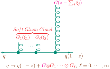
Figure 1: Bloch-Nordsieck soft quanta for an accelerated charge.

an accelerated charge generates a coherent state of very soft massless quanta of the respective gauge field so that one cannot know which of the infinity of possible states one has made in the splitting process $q(1)\rightarrow q(1-z)+G\otimes G_{1}\cdots\otimes G_{\ell},\;\ell=0,\cdots,\infty$ illustrated in Fig. 1. In the new kernels this effect is taken into account by resumming the terms ${\cal O}\left((\alpha_{s}\ln(\frac{q^{2}}{\Lambda^{2}})\ln(1-z))^{n}\right)$ when $z\rightarrow 1$ is the IR limit. From (27) and (1), we see that when the usual kernels are used these terms are generated order-by-order in the solution for the cross section $\sigma$ in (1) so that our resumming them enhances the convergence of the representation in (1) for a given order of exactness in the input perturbative components therein. In the next Section, we illustrate this last remark in the context of the comparison of recent LHC data to NLO parton shower/matrix element matched predictions.

3 Interplay of IR-Improved DGLAP-CS Theory and NLO Shower/ME Precision: Comparison with LHC Data

In the new MC HERWIRI1.031 [9] we have the first realization of the new IR-improved kernels in the HERWIG6.5 [10] environment. Here, using recent LHC data as our baseline, we compare it with HERWIG6.510, both with and without the MC@NLO [11] exact ${\cal O}(\alpha_{s})$ correction to illustrate the interplay between the attendant precision in NLO ME matched parton shower MC’s and the new IR-improvement for the kernels.

More specifically, in Fig. 2 in panel (a) we show for the single $Z/\gamma*$ production at the LHC the comparison between the CMS rapidity data [39] and the MC theory predictions and in panel (b) in the same figure we show the analogous comparison with the ATLAS $P_{T}$ data. Here, the rapidity data are the combined $e^{+}e^{-}-\mu^{-}\mu^{+}$ results and the $p_{T}$ data are those for the bare $e^{+}e^{-}$ case; for, the theoretical framework of our simulations corresponds to these data. We do not as yet have complete realization of all the corrections involved in the other ATLAS data in Ref. [40].

Figure 2: Comparison with LHC data: (a), CMS rapidity data on ($Z/\gamma^{*}$) production to $e^{+}e^{-},\;\mu^{+}\mu^{-}$ pairs, the circular dots are the data, the green(blue) lines are HERWIG6.510(HERWIRI1.031); (b), ATLAS $p_{T}$ spectrum data on ($Z/\gamma^{*}$) production to (bare) $e^{+}e^{-}$ pairs, the circular dots are the data, the blue(green) lines are HERWIRI1.031(HERWIG6.510). In both (a) and (b) the blue(green) squares are MC@NLO/HERWIRI1.031(HERWIG6.510($\rm{PTRMS}=2.2$GeV)). In (b), the green triangles are MC@NLO/HERWIG6.510($\rm{PTRMS}=$0). These are otherwise untuned theoretical results.

These results are better appreciated if they are considered from the perspective of our analysis in Ref. [9] of the FNAL data on the single $Z/\gamma^{*}$ production in $\text{p}\bar{\text{p}}$ collisions at 1.96 TeV.

More precisely, we direct the reader to the results in Fig. 11 of the second paper in Ref. [9]. In that figure, we showed that, when the intrinsic rms $p_{T}$ parameter $\rm{PTRMS}$ is set to 0 in HERWIG6.5, the MC@NLO/HERWIG6.510 simulations give a good fit to the CDF rapidity distribution data [42] therein but they do not give a satisfactory fit to the D0 $p_{T}$ distribution data [43] therein. In contrast, the corresponding simulations for MC@NLO/HERWIRI1.031 give good fits to both sets of data with the $\rm{PTRMS}=0$. Here $\rm{PTRMS}$ corresponds to rms value for an intrinsic Gaussian distribution in $p_{T}$. The authors of HERWIG [41] already have observed that, to get good fits to both sets of data, one may set $\rm{PTRMS}\cong 2$ GeV. Accordingly, in analyzing the new LHC data, we have set $\rm{PTRMS}=2.2$GeV in our HERWIG6.510 simulations while we continue to set PRTMS=0 in our HERWIRI simulations.

We turn now with this perspective to the results in Fig. 2, where we see a confirmation of the finding of the HERWIG authors. One needs to set $\rm{PTRMS}\cong 2\text{GeV}$ [44] in the MC@NLO/HERWIG6510 simulations to get a good fit to both the CMS rapidity data and the ATLAS $p_{T}$ data. We again see that the MC@NLO/HERWIRI1.031 simulations with $\rm{PTRMS}=0$ at LHC give a good fit to the data for both the rapidity and the $p_{T}$ spectra. Quantitatively, we use the $\chi^{2}/\text{d.o.f.}$ as a measure of the goodness of the respective fits. From the results in Fig. 2 we compute that the $\chi^{2}/\text{d.o.f.}$ for the rapidity data and the $\chi^{2}/\text{d.o.f.}$ for the $p_{T}$ data are (.72,.72)((.70,1.37)) for the MC@NLO/HERWIRI1.031(MC@NLO/HERWIG 6510($\rm{PTRMS}$=2.2GeV)) simulations.
The corresponding results are (.70,2.23) for the MC@NLO/HERWIG6510($\rm{PTRMS}$=0) simulations.

To reproduce the LHC data on the $p_{T}$ distribution of the $Z/\gamma^{*}$ in the pp collision the usual DGLAP-CS kernels require the introduction of a hard intrinsic Gaussian distribution in $p_{T}$ inside the proton whereas the IR-improved kernels give in fact a better fit to the data without the introduction of such a hard intrinsic component to the motion of the proton’s constituents. The hardness of this intrinsic $\rm{PTRMS}$ is the issue as this quality of it is entirely ad hoc; it is in disagreement with the results of all successful models of the proton wave-function [45], wherein the scale of the corresponding intrinsic $\rm{PTRMS}$ is found to be $\lesssim 0.4$GeV. More significantly, it contradicts the well-known experimental observation of precocious Bjorken scaling [46, 47]; for, the famous SLAC-MIT experiments on the deep inelastic electron-proton scattering process show that Bjorken scaling occurs already at $Q^{2}=1_{+}$ GeV² for $Q^{2}=-q^{2}$ with q the 4-momentum transfer from the electron to the proton. If the proton constituents really had a Gaussian intrinsic $p_{T}$ distribution with $\rm{PTRMS}\cong 2$GeV, these pioneering SLAC-MIT observations would not be possible. What we advocate now is that the ad hoc “hardness” of the $\rm{PTRMS}\cong 2.2$GeV value is really just a phenomenological representation of the more fundamental dynamics described by the IR-improved DGLAP-CS theory. This raises the following question: “Is possible to tell the difference between the two representations of the data in Fig. 2?”

One expects physically that more detailed observations should be able to distinguish the two representations of the data in Fig. 2. In this connection, in Fig. 3 we show for the $Z/\gamma^{*}$ mass spectrum the MC@NLO/HERWIRI1.031(blue squares) and MC@NLO/HER-
WIG6510($\rm{PTRMS}$=2.2GeV) (green squares) predictions when the decay lepton pairs satisfy the LHC type requirement that their transverse momenta $\{p^{\ell}_{T},p^{\bar{\ell}}_{T}\}$ exceed $20$ GeV.

Figure 3: Normalized vector boson mass spectrum at the LHC for $p_{T}(\text{lepton})>20$ GeV.

From the results in Fig. 3, wherein the peaks differ by 2.2% for example, we see that the high precision data such as the LHC ATLAS and CMS experiments will have (each already has over $5\times 10^{6}$ lepton pairs) would allow one to distinguish between the two sets of theoretical predictions.

Continuing in this direction with the discussion, we see that the main differences between the three predictions in Fig. 2 (b) occur in the regime below $10$ GeV/c. To better probe this latter regime, we make a more detailed snap-shot of it in which we plot in Fig. 4 the three respective featured theory predictions with the finer binning of $0.5$GeV/c instead of the $3.0$GeV/c binning used in Fig. 2 (b).

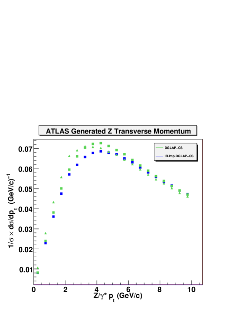
Figure 4: Normalized vector boson $p_{T}$ spectrum at the LHC for the ATLAS cuts as exhibited in Fig. 2 for the same conventions on the notation for the theoretical results with the vector boson $p_{T}<10$ GeV to illustrate the differences between the three predictions.

The results in Fig. 4 show that the three theoretical predictions have significant differences in the shapes that are testable with the precise data that will be available to the ATLAS and CMS experiments. We would again encourage experimentalists to pursue the measurements of both $p_{T}$ and $\phi_{\eta}^{*}$ spectra as these will both be very useful in establishing the correct theoretical approach to the respective LHC observations. We will pursue elsewhere [12] other such detailed observations that may also reveal the differences between the two descriptions of parton shower physics. In this connection especially, we continue to await the release of the entire data sets from ATLAS and CMS.

4 Conclusions

What we have shown is the following. The realization of IR-improved DGLAP-CS theory in HERWIRI1.031, when used in the MC@NLO/HERWIRI1.031 exact ${\cal O}(\alpha_{s})$ ME matched parton shower framework, affords one the opportunity to explain, on an event-by-event basis, both the rapidity and the $p_{T}$ spectra of the $Z/\gamma^{*}$ in pp collisions in the recent LHC data from CMS and ATLAS, respectively, without the need of an unexpectedly hard intrinsic Gaussian $p_{T}$ distribution with rms value of $\rm{PTRMS}\cong 2$ GeV in the proton’s wave function. Our view is that this can be interpreted as providing a rigorous basis for the phenomenological correctness of such unexpectedly hard distributions insofar as describing these data using the usual unimproved DGLAP-CS showers is concerned. Accordingly, we have proposed that comparison of other distributions such as the invariant mass distribution with the appropriate cuts and the more detailed $Z/\gamma^{*}$ $p_{T}$ spectra in the regime below $10.0$GeV be used to differentiate between these phenomenological representations of parton shower physics in MC@NLO/HERWIG6510 and the fundamental description of the parton shower physics in MC@NLO/HERWIRI1.031. We have further emphasized that the precociousness of Bjorken scaling argues against the fundamental correctness of the hard scale intrinsic $p_{T}$ ansatz with the unexpectedly hard value of $\rm{PTRMS}\cong 2$ GeV, as do the successful models [45] of the proton’s wave function, which would predict this value to be $\lesssim 0.4$GeV. As an added bonus, we have pointed-out that the fundamental description in MC@NLO/HERWIRI1.031 can be systematically improved to the NNLO parton shower/ME matched level – a level which we anticipate is a key ingredient in achieving the (sub-)1% precision tag for such processes as single heavy gauge boson production at the LHC.

Evidently, relative to what one could achieve from the fundamental representation of the corresponding physics via IR-improved DGLAP-CS theory as it is realized in HERWIRI1.031 when employed in MC@NLO/HERWIRI1.031 simulations, the use of ad hoc hard scales in models would compromise any discussion of the attendant theoretical precision. We are pursuing additional cross checks of the MC@NLO/HERWIRI1.031 simulations against the LHC data.

In our discussion, we have also spent some amount of time discussing alternative approaches to the type of resummation embodied in the IR-improved DGLAP-CS theory; for, some of these approaches are in wide use. What we conclude is that the physical precisions of these approaches(see Sect. 2), which are based on Refs. [23, 24, 25, 26], are above the 1% precision tag that we aspire, even though there is no contradiction between our exact approach and these more approximate methods.

In closing, two of us (A.M. and B.F.L.W.) thank Prof. Ignatios Antoniadis for the support and kind hospitality of the CERN TH Unit while part of this work was completed.

References

- [1] F. Gianotti, in Proc. ICHEP2012, in press; J. Incandela, ibid., 2012, in press; G. Aad et al., Phys. Lett. B716 (2012) 1, arXiv:1207.7214; D. Abbaneo et al., ibid.716 (2012) 30, arXiv:1207.7235.
- [2] F. Englert and R. Brout, Phys. Rev. Lett. 13 (1964) 312; P.W. Higgs, Phys. Lett. 12 (1964) 132; Phys. Rev. Lett. 13 (1964) 508; G.S. Guralnik, C.R. Hagen and T.W.B. Kibble, ibid. 13 (1964) 585.
- [3] B.F.L. Ward, S.K. Majhi and S.A. Yost, in PoS(RADCOR2011) (2012) 022.
- [4] C. Glosser, S. Jadach, B.F.L. Ward and S.A. Yost, Mod. Phys. Lett. A 19(2004) 2113; B.F.L. Ward, C. Glosser, S. Jadach and S.A. Yost, in Proc. DPF 2004, Int. J. Mod. Phys. A 20 (2005) 3735; in Proc. ICHEP04, vol. 1, eds. H. Chen et al.,(World. Sci. Publ. Co., Singapore, 2005) p. 588; B.F.L. Ward and S. Yost, preprint BU-HEPP-05-05, in Proc. HERA-LHC Workshop, CERN-2005-014; in Moscow 2006, ICHEP, vol. 1, p. 505; Acta Phys. Polon. B 38 (2007) 2395; arXiv:0802.0724, PoS(RADCOR2007)(2007) 038; B.F.L. Ward et al., arXiv:0810.0723, in Proc. ICHEP08; arXiv:0808.3133, in Proc. 2008 HERA-LHC Workshop,DESY-PROC-2009-02, eds. H. Jung and A. De Roeck, (DESY, Hamburg, 2009)pp. 180-186, and references therein.
- [5] G. Altarelli and G. Parisi, Nucl. Phys. B126 (1977) 298; Yu. L. Dokshitzer, Sov. Phys. JETP 46 (1977) 641; L. N. Lipatov, Yad. Fiz. 20 (1974) 181; V. Gribov and L. Lipatov, Sov. J. Nucl. Phys. 15 (1972) 675, 938; see also J.C. Collins and J. Qiu, Phys. Rev. D39 (1989) 1398.
- [6] C.G. Callan, Jr., Phys. Rev. D2 (1970) 1541; K. Symanzik, Commun. Math. Phys. 18 (1970) 227, and in Springer Tracts in Modern Physics, 57, ed. G. Hoehler (Springer, Berlin, 1971) p. 222; see also S. Weinberg, Phys. Rev. D8 (1973) 3497.
- [7] B.F.L. Ward, Adv. High Energy Phys. 2008 (2008) 682312.
- [8] B.F.L. Ward, Ann. Phys. 323 (2008) 2147.
- [9] S. Joseph et al., Phys. Lett. B685 (2010) 283; Phys. Rev. D81 (2010) 076008.
- [10] G. Corcella et al., hep-ph/0210213; J. High Energy Phys. 0101 (2001) 010; G. Marchesini et al., Comput. Phys. Commun.67 (1992) 465.
- [11] S. Frixione and B.Webber, J. High Energy Phys. 0206 (2002) 029; S. Frixione et al., arXiv:1010.0568; B. Webber, talk at CERN, 03/30/2011; S. Frixione, talk at CERN, 05/04/2011.
- [12] A. Mukhopadhyay et al., to appear.
- [13] M. Bahr et al., arXiv:0812.0529 and references therein.
- [14] T. Sjostrand, S. Mrenna and P. Z. Skands, Comput. Phys. Commun. 178 (2008) 852-867.
- [15] T. Gleisberg et al., J.High Energy Phys. 0902 (2009) 007.
- [16] P. Nason, J. High Energy Phys. 0411 (2004) 040.
- [17] S. Majhi et al., Phys. Lett. B 719 (2013) 367.
- [18] See for example S. Jadach et al., in Physics at LEP2, vol. 2, (CERN, Geneva, 1995) pp. 229-298.
- [19] D. R. Yennie, S. C. Frautschi, and H. Suura, Ann. Phys. 13 (1961) 379; see also K. T. Mahanthappa, Phys. Rev. 126 (1962) 329, for a related analysis.
- [20] See also S. Jadach and B.F.L. Ward, Comput. Phys. Commun. 56(1990) 351; Phys.Lett. B 274 (1992) 470; S. Jadach et al., Comput. Phys. Commun. 102 (1997) 229; S. Jadach, W. Placzek and B.F.L Ward, Phys. Lett. B 390 (1997) 298; S. Jadach, M. Skrzypek and B.F.L. Ward,Phys. Rev. D 55 (1997) 1206; S. Jadach, W. Placzek and B.F.L. Ward, Phys. Rev. D 56 (1997) 6939; S. Jadach, B.F.L. Ward and Z. Was,Phys. Rev. D 63 (2001) 113009; Comp. Phys. Commun. 130 (2000) 260; ibid.124 (2000) 233; ibid.79 (1994) 503; ibid.66 (1991) 276; S. Jadach et al., ibid.140 (2001) 432, 475.
- [21] B.F.L. Ward and S. Jadach, Mod. Phys. Lett. A14 (1999) 491.
- [22] J.G.M. Gatheral, Phys. Lett. B 133 (1983) 90.
- [23] G. Sterman, Nucl. Phys. B 281, 310 (1987); S. Catani and L. Trentadue, Nucl. Phys. B 327, 323 (1989); ibid. 353, 183 (1991).
- [24] See for example C. W. Bauer, A.V. Manohar and M.B. Wise, Phys. Rev. Lett. 91 (2003) 122001; Phys. Rev. D 70 (2004) 034014; C. Lee and G. Sterman, Phys. Rev. D 75 (2007) 014022.
- [25] J.C. Collins and D.E. Soper, Nucl. Phys. B193 (1981) 381; ibid.213(1983) 545; ibid. 197(1982) 446.
- [26] J.C. Collins, D.E. Soper and G. Sterman, Nucl. Phys. B250(1985) 199; in Les Arcs 1985, Proceedings, QCD and Beyond, pp. 133-136.
- [27] S. Hassani, in Proc. Recntres de Moriond EW, 2013, in press; H. Yin, ibid., 2013, in press; G. Aad et al., arXiv:1211.6899, and references therein.
- [28] C. Balazs and C. Yuan, Phys. Rev. D56 (1997) 5558.
- [29] G. Ladinsky and C. Yuan, Phys. Rev. D50 (1994) 4239.
- [30] F. Landry et al., Phys. Rev. D63 (2003) 073016.
- [31] Yu.L. Dokshitser, D.I. D’yakonov and S.I. Troyan, Phys. Lett. B78 (1978) 290; Proc. 13th Winter School of the LPNI, Leneingrad(1978); Phys. Rept. 58 (1980) 271; G. Parisi and R. Petronzio, Nucl. Phys. B 154 (1979) 427; G. Curci, M. Greco and R. Srivastava, Phys. Rev. Lett. 43 (1979) 834; Nucl. Phys. B 159 (1979) 451; P. Chiappetta and M. Greco, Nucl.Phys. B199 (1982) 77; ibid. 221 (1983) 268; Phys. Lett. B135 (1984) 187; F. Halzen, A.D. Martin and D.M. Scott, Phys. Rev. D25 (1982) 754; P. Aurenche and R. Kinnunen, Phys. Lett. B 135 (1984) 493; A. Nakamura, G. Pancheri and Y. Srivastava, Z. Phys. 21 (1984) 243; G. Altarelli, R.K. Ellis, M. Greco and G. Martinelli, Nucl. Phys. B 246 (1984) 12.
- [32] C. Davies, B. Webber and W. Stirling, Nucl. Phys. B256 (1985) 413.
- [33] A. Banfi et al., Phys. Lett. B715(2012) 152 and references therein.
- [34] T. Becher, M. Neubert and D. Wilhelm, arXiv:1109.6027; T. Becher, M. Neubert, Eur. Phys. J. C71 (2011) 1665, and references therein.
- [35] B.I. Ermolaev, M. Greco and S.I. Troyan, PoS DIFF2006 (2006) 036, and references therein.
- [36] A. Banfi et al., Eur. Phys. J. C71 (2011) 1600.
- [37] G. Altarelli, R.D. Ball and S. Forte, PoS RADCOR2007 (2007) 028.
- [38] F. Bloch and A. Nordsieck, Phys. Rev. 52 (1937) 54.
- [39] S. Chatrchyan et al., arXiv:1110.4973; Phys. Rev. D85 (2012) 032002.
- [40] G. Aad et al., arXiv:1107.2381; Phys. Lett. B705 (2011) 415.
- [41] M. Seymour, “Event Generator Physics for the LHC”, CERN Seminar, 2011.
-
[42]
C. Galea, in Proc. DIS 2008, London, 2008,
http://dx.doi.org/10.3360/dis.2008.55. - [43] V.M. Abasov et al., Phys. Rev. Lett. 100, 102002 (2008).
- [44] P. Skands, private communication, 2011, finds a similar behavior in PYTHIA8 simulations.
- [45] R.P. Feynman, M. Kislinger and F. Ravndal, Phys. Rev. D3 (1971) 2706; R. Lipes, ibid.5 (1972) 2849; F.K. Diakonas, N.K. Kaplis and X.N. Mawita, ibid. 78 (2008) 054023; K. Johnson, Proc. Scottish Summer School Phys. 17 (1976) p. 245; A. Chodos et al., Phys. Rev. D9 (1974) 3471; ibid. 10 (1974) 2599; T. DeGrand et al., ibid. 12 (1975) 2060.
- [46] See for example R.E. Taylor, Phil. Trans. Roc. Soc. Lond. A359 (2001) 225, and references therein.
- [47] J. Bjorken, in Proc. 3rd International Symposium on the History of Particle Physics: The Rise of the Standard Model, Stanford, CA, 1992, eds. L. Hoddeson et al. (Cambridge Univ. Press, Cambridge, 1997) p. 589, and references therein.