How well do we know the polar hydrogen distribution on the Moon?

Abstract

A detailed comparison is made of results from the Lunar Prospector Neutron Spectrometer (LPNS) and the Lunar Exploration Neutron Detector Collimated Sensors for EpiThermal Neutrons (LEND CSETN). Using the autocorrelation function and power spectrum of the polar count rate maps produced by these experiments, it is shown that the LEND CSETN has a footprint that is at least as big as would be expected for an omni-directional detector at an orbital altitude of $50$ km. The collimated flux into the field of view of the collimator is negligible. Arguments put forward asserting otherwise are considered and found wanting for various reasons. The maps of lunar polar hydrogen with the highest contrast, i.e. spatial resolution, are those resulting from pixon image reconstructions of the LPNS data. These typically provide weight percentages of water equivalent hydrogen that are accurate to $30\%$ within the polar craters.

TEODORO et al. ¹ BAER, NASA Ames Research Center, Moffett Field, CA 94035-1000, USA (luis.f.teodoro@nasa.gov), ² Institute for Computational Cosmology, Department of Physics, Durham University, Science Laboratories, South Road, Durham DH1 3LE, UK, ³ Planetary Systems Branch, Space Sciences and Astrobiology Division, MS 245-3, NASA Ames Research Center, Moffett Field, CA 94035-1000, USA, ⁴ Planetary Science Institute, 1700 E. Fort Lowell, Suite 106, Tucson, AZ 85719, USA, ⁵ Johns Hopkins University Applied Physics Laboratory, Laurel, MD 20723, USA.

Gindraft=false

1 Introduction

The presence and distribution of hydrogen near the lunar surface is a matter of considerable interest (Watson et al., 1961; Arnold, 1979). This ancient surface, like that of Mercury, contains a record of the history of the inner solar system, and the likely association of hydrogen with water molecules can provide insights into the delivery and retention of volatile molecules over the past few billion years (Lawrence et al., 2013; Paige et al., 2013; Neumann et al., 2013).

Remote sensing of the epithermal neutron flux coming from the lunar surface provides a measure of the hydrogen abundance in the top metre or so of the lunar regolith (Lingenfelter et al., 1961; Metzger and Drake, 1990; Feldman et al., 1991). Cosmic rays interacting with nuclei in the regolith create energetic, fast neutrons that subsequently evolve and lose energy through inelastic and elastic collisions with other nuclei. Some of these neutrons escape into space before losing enough energy to be reabsorbed into another nucleus, and this leakage flux contains information about the nuclear content of the upper regolith. Hydrogen provides a very effective moderator of intermediate energy, epithermal neutrons that predominantly lose energy through elastic scattering. Consequently, the presence of hydrogen in the top metre of regolith leads to a relatively low flux of epithermal neutrons leaking from the surface.

Pioneering work in this subject was performed by those working with the Lunar Prospector Neutron Spectrometer (LPNS), who mapped the lunar neutron flux at fast, epithermal and thermal energies (Feldman et al., 1998a; Elphic et al., 1998; Feldman et al., 1998b). Fast neutrons provide a map of the mean atomic mass (Gasnault et al., 2001), while thermal neutrons identify regions with higher abundances of neutron-absorbing nuclei such as iron, titanium, gadolinium and samarium. A deficit of epithermal neutrons is seen over the mare regions, because the lower energy epithermal neutrons are sensitive to the neutron absorbing nuclei (Lawrence et al., 2006). While this is not important for the polar regions, which have a feldspathic composition characteristic of the lunar highlands, when making a global hydrogen map Feldman et al. (2000) introduced a quantity $epi^{*}$ to correct for the effects of these non-hydrogen absorbers at low latitudes. Nearer the poles, the main aspect of composition driving the epithermal neutron count rate is hydrogen and the LPNS results showed reduced polar epithermal neutron count rates, implying the presence of polar hydrogen.

With the $\sim 45$ km footprint size of the omni-directional LPNS (Maurice et al., 2004) and the inevitable stochastic noise present in the data, it was difficult to determine if the dips in count rate were associated with the relatively small permanently shaded regions (PSRs) that might be expected to host water ice deposits. Consequently, pixon image reconstruction techniques (Pina and Puetter, 1993; Eke, 2001) were employed to enhance the information that could be extracted from the data. Using the method introduced in Elphic et al. (2007), Eke et al. (2009) were the first to show that the data favoured a scenario where the hydrogen was, on average, concentrated into the PSRs. This analysis was improved using updated maps of the PSRs by Teodoro et al. (2010), whose maps were used in the targeting of the Lunar Crater Observation and Sensing Satellite (LCROSS) in its successful bid to find water ice in the Cabeus crater (Colaprete et al., 2010).

NASA’s Lunar Precursor Robotic Program was intended to “pave the way for eventual permanent human presence on the Moon” (Chin et al., 2007). The first mission of this program was the Lunar Reconnaissance Orbiter (LRO), which employs “six individual instruments to produce accurate maps and high-resolution images of future landing sites, to assess potential lunar resouces, and to characterize the radiation environment” (Chin et al., 2007). One of these instruments is the Lunar Exploration Neutron Detector (LEND), with a primary objective being to “determine hydrogen content of the subsurface at the polar regions with spatial resolution of $10$ km and with sensitivity to concentration variations of 100 parts per million at the poles” (Chin et al., 2007). Rather than taking omni-directional measurements and using software to enhance the resulting images, as was done with the LPNS, the LEND Collimated Sensors for EpiThermal Neutrons (CSETN) represent an attempt at a hardware solution to the challenge of making sharper maps of the lunar epithermal neutron count rate. This was to be achieved using a two-layer collimator with an outer layer of polyethylene to moderate the neutrons and an inner layer of boron to absorb them (Mitrofanov et al., 2008).

Prior to launch, there was a study anticipating how the LEND CSETN might perform. Lawrence et al. (2010) used Monte Carlo modelling based on experience gained from work with the LPNS to infer that the neutron count rate through the small field of view of the collimator was going to be a rather low $0.18$ neutrons per second. However, this disagreed with the estimate from Mitrofanov et al. (2008), who found a value of $0.9$ per second.

Analyses of orbital LEND CSETN data have resulted in discordant inferences concerning the behaviour of the collimator. Mitrofanov et al. (2010) claimed that the LEND CSETN was receiving “about $1.9$” collimated neutrons per second. On the basis of this interpretation, Mitrofanov et al. (2010) concluded that epithermal neutron suppressions, and by implication enhanced hydrogen concentrations, were not spatially coincident with permanently shaded regions. In response, Lawrence et al. (2011) contended that the LEND CSETN count rate was dominated by an uncollimated high energy epithermal neutron component. As a consequence, Lawrence et al. (2011) concluded that the LEND CSETN data did not support the polar hydrogen distributions inferred by Mitrofanov et al. (2010). A more comprehensive likelihood analysis of the time series data was performed by Eke et al. (2012), who considered the three different components contributing to the LEND CSETN count rate: the lunar collimated component, the lunar uncollimated component, i.e. neutrons from ouside the collimator field of view on the Moon that scatter off spacecraft material into the detector, and neutrons generated by cosmic rays striking spacecraft material itself. Taking into account the three different components contributing to the LEND CSETN count rate and how they should vary with longitude, latitude and spacecraft altitude, Eke et al. (2012) showed that the collimated count rate represented less than about $10\%$ of the lunar-derived neutrons, allowing for potential systematic uncertainties. The uncollimated lunar neutrons, which provide a spatially varying background, dominated the count rate from the Moon. However, more than half of the LEND CSETN count rate is derived from cosmic rays striking the spacecraft itself (Eke et al., 2012), so fewer than $5\%$ of the detected neutrons were actually lunar and collimated. Eke et al. (2012) determined that $1\%$ is the most likely fraction of the detected neutrons that are lunar and collimated, meaning that the effective footprint of the LEND CSETN will be set by the uncollimated lunar background component and is likely to be at least $\sim 50$ km in size. More recently, a number of papers have appeared (Litvak et al., 2012a; Sanin et al., 2012; Mitrofanov et al., 2012; Litvak et al., 2012b; Boynton et al., 2012) that contain assertions to the effect that the LEND CSETN is producing a map with $10$ km spatial resolution.

Given the importance for the planning of future missions, it is imperative that the capability of the LEND CSETN is clarified for decision-makers outside the field of planetary neutron studies. The purpose of this paper is to determine empirically the instrumental spatial resolution and the background contamination in the data, and hence the ability to map hydrogen near the lunar poles, of the LEND CSETN. This will be achieved using techniques that are new to planetary neutron spectroscopy, but well established in other scientific fields.

In the next section, two statistical measures will be introduced to characterise the performance of a detector given the output map it produces. These will then be applied in Section 3 to the data sets from both the LPNS and LEND CSETN in order to compare the relative performance of these two detectors. The various arguments put forward by authors in support of statements about the proper functioning of the LEND CSETN are investigated in detail in Section 4. The results from this study are discussed in Section 5, and conclusions drawn in Section 6.

2 Characterising detector performance

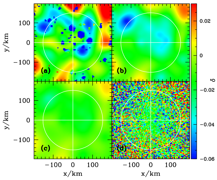
Figure 1: Maps illustrating the degradation of information during the process of making an observation. Panel (a) shows an example input map of fractional count rate difference, $\delta$. The map resulting from smoothing with the spatial response function of the LPNS at $30$ km altitude is shown in (b). Including a uniform background with the same mean count rate as that in the input map leads to the results in panel (c), and a noisy realisation of this, which is what would be measured, is shown in (d).

There are three important ways in which measured maps of epithermal neutron count rate will be degraded representations of what actually leaves the lunar surface. A detector orbiting above the Moon does not solely receive neutrons from directly beneath it. Omni-directional detectors count neutrons coming from all parts of the Moon out to the horizon, whereas an ideal collimated detector would have a restricted, but still extended, field of view. In both cases, the measured epithermal neutron map will be blurred by the extended spatial response function, or ‘footprint’, of the detector. The blurring caused by the LPNS at an altitude of $30$ km is illustrated by the difference between the images in panels (a) and (b) in Fig. 1. Rather than showing a count rate map, these maps show the fractional difference,

$$\delta({\mathbf{x}})=\frac{c({\mathbf{x}})-\bar{c}}{\bar{c}},$$ (1)

where $c({\mathbf{x}})$ is the count rate in the two-dimensional map at position ${\mathbf{x}}$ and $\bar{c}$ represents the mean count rate per pixel in the observed region. This statistic is invariant under changes in detector efficiency or cosmic ray flux and thus represents a convenient way to compare detectors. Panel (a) is a pixon reconstruction of the LPNS data in the south polar region (Teodoro et al., 2010), with the south pole at the centre of the image, and adopting a polar stereography projection. The mean count rate, $\bar{c}$, is defined in the region $|x|,|y|<600$ km.

The second important degradation introduced during the measurement process arises from the production of neutrons local to the detector due to cosmic rays striking the spacecraft itself. The resulting neutrons have nothing to do with the lunar surface composition and provide a uniform spatial background that dilutes the contrast present in the lunar signal, as shown by the difference between panels (b) and (c) in Fig. 1. A background count rate equal to the mean in the blurred image has been assumed. This is more appropriate for the LEND CSETN than the LPNS because, while the LPNS was on a boom $2.5$ m away from the main body of a relatively small spacecraft, the LEND is right next to the much more massive LRO. This uniform background is distinct from the background due to the uncollimated lunar neutrons that are scattered off spacecraft material into the LEND CSETN detector and provide a spatially varying background.

The final aspect of the measurement procedure that acts to obscure the underlying lunar signal is the fact that integration times are finite, leading to inevitable stochastic noise in the collected data. Panel (d) of Fig. 1 shows how this noise impacts upon the fractional count rate difference for a sampling similar to that made by LP. The fact that pixels near to the pole receive more visits and suffer less statistical noise is clearly visible in this map.

It is evident from Fig. 1 that all three of these aspects of detector performance leave strong imprints on the measured data set. Thus, determining the relative merits of the LPNS and LEND CSETN boils down to choosing appropriate statistical measures that are sensitive to each of these contributing factors. In this way the size of the instrumental spatial footprint, the background contamination, and the statistical noise can be estimated empirically from the maps constructed using data from these two experiments.

Two powerful statistical measures that are widely used in many different scientific disciplines to quantify the properties of continuous stochastic fields such as $\delta({\mathbf{x}})$, are the power spectrum and the autocorrelation function (Peebles, 1980; Monin et al., 2007). Both of these quantities encode information about the amount of structure contained in a map on a variety of different spatial scales. In the field of Space Science, these statistical measures have been used in studies of the lunar gravitational potential (Wieczorek and Phillips, 1998), modeling of martian dunes dynamics (Narteau et al., 2009), helioseismology (Christensen-Dalsgaard et al., 1985), X-ray variability from black hole accretion discs (McHardy et al., 2006), galaxy clustering (Cole et al., 2005; Eisenstein et al., 2005) and the cosmic microwave background (Planck Planck Collaboration, 2013) to name a few examples.

2.1 The autocorrelation function

The autocorrelation function of a map is a measure of the similarity between values in pixels at different relative positions. It is defined by

$$\xi(r=|\mathbf{r}|)\equiv\left<\delta\left(\mathbf{x}\right)\delta\left(\mathbf{x}-\mathbf{r}\right)\right>$$ (2)

where the average is over pixel position $\mathbf{x}$ and isotropy guarantees that $\xi(r)$ is independent of the direction of the separation of the pixels, $\mathbf{r}$. This function depends not only on the intrinsic clustering properties of the fractional count rate differences, but also on both the smoothing length imposed on the data by the instrumental spatial resolution and the amount of uniform background that is introduced.

In formal terms, smoothing can be represented by the convolution

$$\delta_{S}(\mathbf{x})=\int_{\mbox{\scriptsize{over all space }}}\delta(\mathbf{x}^{\prime})\,W\left(\mathbf{x}-\mathbf{x}^{\prime}\right)\,d^{2}\mathbf{x}^{\prime},$$ (3)

where the smoothing kernel is normalised such that

$$\int W\left(\mathbf{x}-\mathbf{x}^{\prime}\right)\,d^{2}\mathbf{r}=1,$$ (4)

and $\delta_{S}(\mathbf{x})$ represents the smoothed map. Qualitatively, on scales smaller than the size of the kernel the correlation function will be approximately flat. For scales larger than a few smoothing lengths the correlation functions of the smoothed and unsmoothed maps coincide within the measurement error. This is illustrated in Fig. 2, where the solid and dashed lines represent $\xi(r)$ for the unsmoothed and smoothed maps shown in Fig. 1 panels (a) and (b) respectively. The smoothing kernel used was

$$W(r)=\frac{A}{\left(1+\left(r/\sigma\right)^{2}\right)^{2}},$$ (5)

with $\sigma=35$ km to mimic the omni-directional LPNS at $30$ km altitude and $A$ being a normalisation constant (Maurice et al., 2004). These autocorrelation functions have been calculated for polar data on the projection grid going out to $|x|,|y|=600$ km from the south pole in $5$ km square pixels (Fig. 1 shows the central ninth of this region), using a similar length of zero-padding to avoid wrap-around issues when using Fast Fourier Transforms in the computation.

Figure 2: The impact of the measurement process on the autocorrelation function of polar neutron maps. Curves show the autocorrelation functions for the input map (solid), the blurred map without any uniform background included (dashed), and after a uniform background has been added (dotted). These correspond to panels a, b and c in Fig. 1). Filled circles represent the autocorrelation function measured from the particular noisy realisation shown in panel (d) of Fig. 1, with error bars representing the uncertainty due to sample variance, inferred using many different noisy realisations.

The dotted line in Fig. 2 represents the effect of a uniform background with a count rate equal to that of the mean lunar signal. This amount of background is far larger than was suffered by the LPNS, but almost matches that experienced by the LEND CSETN. The fluctuations in the smoothed map become diluted by a factor of $2$, meaning that the autocorrelation function is suppressed on all scales by a factor of $4$. Panel (c) of Fig. 1 shows the associated loss of contrast in the map. $\xi(r)$ for the noisy map in panel (d) of Fig. 1 is represented by the points in Fig. 2. As the noise is assumed to be spatially uncorrelated, only the value of $\xi$ at zero separation (not shown on this log plot) is systematically changed by the presence of noise. The larger separation values merely have statistical noise added to them. These are represented by the error bars, which are determined from the scatter between the individual measurements when many different noisy realisations of the same underlying map are made.

2.2 The power spectrum

The power spectrum is just the Fourier transform of the autocorrelation function and represents an alternative way of showing which spatial scales contain information. In terms of the wavenumber $\mathbf{k}=2\pi/\mathbf{\lambda}$, where $\mathbf{\lambda}$ represents the corresponding wavelength in two-dimensional pixel space, the power spectrum is

$$P(k=\left|\mathbf{k}\right|)\equiv\left<\left|\mathbf{\delta_{k}}\right|^{2}\right>,$$ (6)

with $\mathbf{\delta_{k}}$ representing the amplitude of the $\mathbf{k}$th mode in the Fourier decomposition of the map of $\delta(\mathbf{x})$ and the average is over modes with the same wavenumber $k$.

The power spectra for the four maps in Fig. 1 are given in Fig. 3. The removal of power at small scales resulting from blurring with the instrumental footprint manifests itself at large wavenumbers. Once again the uniform background produces a scale-independent reduction of the power by a factor of four. However, unlike the case for the autocorrelation function, where the stochastic measurement noise was confined to the zero separation signal at $\xi(0)$, this delta function transforms to a constant in wavenumber space. Consequently, at small scales (large $k$) where the noise overwhelms what remains of the fluctuations in fractional count rate difference, the power spectrum goes flat, identifying precisely the level of statistical noise in the map.

The maps from the LPNS or LEND CSETN data sets can be considered as the result of the measurement process described in this section. Both the autocorrelation function and power spectrum of the resulting maps will provide complementary and comprehensive views of the impact that the detectors have had on the intrinsic lunar count rate map. In the following section, these two statistical estimators will be employed to quantify how well we know the lunar hydrogen distribution.

Figure 3: The impact of the measurement process on the power spectrum of polar neutron maps. Solid, dashed and dotted lines show the power spectra for the input map and blurred maps, with and without a uniform background added respectively. Filled circles represent the power spectrum of the particular noisy realisation shown in panel (d) of Fig. 1, with error bars representing the uncertainty due to sample variance, inferred using many different noisy realisations.

3 Results for lunar neutron data sets

Data from the Geosciences Node of NASA’s Planetary Data System (PDS) were used to create epithermal neutron maps from both the LPNS and LEND CSETN experiments. The time series Reduced Data Records for the LEND CSETN were processed almost as described by Boynton et al. (2012), with a few notable exceptions. Table 2 of that paper describes the impact that the various cuts on the data have for the number of one-second data records that form part of the analysis. However, the quoted number of total raw records exceeds the number of seconds during the claimed period. Thus, this is impossible to replicate. A couple of other differences in the reduction procedure adopted here are that an extra factor of $A_{i,j}$ has been included on the denominator of both equations (2) and (7), $A_{i,j}$ being the count rate normalisation of the $i$th sensor during the $j$th switch-on period. Without this extra factor these equations are dimensionally incorrect. One additional important part of the Boynton et al. (2012) data reduction procedure, not detailed in that paper, is how variances are calculated for time series records where a subset of the four sensors are working and they happen to record zero counts. Equation (9) of Boynton et al. (2012) appears to suggest that this involves the ratio $(0/0)^{2}$, which is not defined. The following equation has been implemented here to use individual sensor normalisations $A_{i}^{0}$ to convert the individual variances $\sigma_{i,j}^{2}$ to that on the total ‘adjusted count rate’, $R$, via

$$\sigma_{R}^{2}=\sum_{on}\sigma_{i,j}^{2}\left(\frac{\sum_{all}A_{i}^{0}}{\sum_{on}A_{i}^{0}}\right)^{2}.$$ (7)

Presumably Boynton et al. (2012) performed a similar procedure. Other than these apparent modifications, the treatment of Solar Energetic Particle events, outlier events, off-nadir measurements, instrumental warm-up and cosmic ray variation has followed the procedure outlined by Boynton et al. (2012). Reassuringly, the results shown here are very similar to those found using the alternative, independent analysis pipeline introduced by Eke et al. (2012).

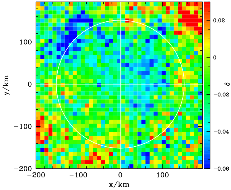
Figure 4: Map of the south pole LPNS fractional count rate difference using $10$ km pixels and data from the $30$ km orbital altitude period. The white circle represents a latitude of $-85^{\circ}$. Statistical uncertainties on the values are $\sim 0.01$ at $-88^{\circ}$, increasing to $\sim 0.015$ at $-85^{\circ}$S. Note that the LPNS data on the PDS has had a small, $\sim 7\%$ (Maurice et al., 2004) uniform background component removed.

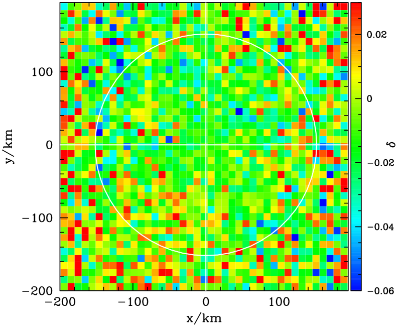
Figure 5: Map of the south pole LEND CSETN fractional count rate difference using $10$ km pixels. The white circle represents a latitude of $-85^{\circ}$. Unlike for the LPNS data on the PDS, the LEND CSETN have not had any uniform background removed. Statistical uncertainties on the values are $\sim 0.01$ at the pole, increasing to $\sim 0.02$ at $-85^{\circ}$.

Figures 4 and 5 show maps of the fractional count rate difference in the vicinity of the lunar south pole made using low-altitude LPNS epithermal neutron (seven months) and LEND CSETN ($\sim$ 21 months) data respectively. It should be noted that the $7\%$ uniform spacecraft background has been removed from the LPNS map (Maurice et al., 2004), whereas the large uniform spacecraft background is still present in the LEND CSETN PDS data. The pixels used are $10$ km on a side. The Cabeus region is clearly seen in the LPNS map as the area of relatively low count rate just over $5^{\circ}$ from the pole in the upper left part of the map. This is very much less pronounced in the LEND CSETN map, which does however have a single $10\times 10$ km² pixel with count rate depressed by at least $6\%$ in the Shoemaker crater on the line $y=x$ at latitude $-88^{\circ}$. The comparison between these two maps, made using all available data in the same region with the same pixellation and the recommended data reduction procedures for the two different experiments, already makes clear that the LPNS produces a map with significantly more contrast than the LEND CSETN. Removing an appropriate uniform spacecraft background from the LEND CSETN map enhances the contrast present in the map, but also makes the map look much noisier. Given the clear differences in the information contents present in the maps for the two different detectors, it is of interest to apply the statistical estimators described in the previous section to determine what can be learned about these results. Figure 6 shows the autocorrelation functions for LPNS data, from both high ($100$ km) and low ($30$ km) altitude periods and that from the LEND CSETN at its altitude of $50$ km. $5$ km square pixels in a region out to $|x|,|y|<600$ km from the pole are used. This large area improves the statistical uncertainties, but the conclusions do not change when only the central ninth of that region (i.e. $|x|,|y|<200$ km), shown in Figs. 4 and 5 with $10$ km square pixels, is chosen. Even if the uniform spacecraft background comprised a fraction $f_{\rm b}=0.54$ of the LEND CSETN count rate, as advocated by Eke et al. (2012) and taking into account the fact that this polar region is slightly different from the entire surface value of $f_{\rm b}=0.535$, and the autocorrelation function were boosted by a factor $1/(1-f_{\rm b})^{2}$, then it would still lie significantly below that from the LPNS at low altitude. It would however increase to have a signal comparable with the high altitude LPNS autocorrelation function. This implies that the footprint of the LEND CSETN is similar to that of the LPNS when it was at an altitude of $100$ km.

The curves in Fig. 6 are constructed by assuming that the intrinsic map of the lunar south pole epithermal neutron count rate is that given by the pixon reconstructions of Teodoro et al. (2010). As the higher energy neutrons detected by the LEND CSETN reflect hydrogen variations in an almost identical way to the lower energy epithermal neutrons measured by the LPNS (Lawrence et al., 2011), it is reasonable to use this map for modelling the polar data from the LEND CSETN. The intrinsic map is observed, by blurring with a footprint defined by $\sigma$, adding a uniform background, and including stochastic noise based upon the observation times in the different pixels for the different experiments. One hundred different random noisy realisations are created and the mean of the results from these forms the curve. The error bars on the curves show the scatter between individual realisations. The curves for LPNS assume $\sigma=35$ km and $101$ km for the low and high altitude cases respectively, and that there is no unaccounted for uniform spacecraft background. To fit the LEND CSETN data, the model curve has included a uniform spacecraft background count rate fraction of $f_{\rm b}=0.54$, and made a composite detector footprint that includes a collimated fraction with footprint $10$ km of $f_{\rm c}=0.01$ and the remaining uncollimated lunar flux is collected with a footprint having $\sigma=90$ km. This is significantly broader than the footprint of an omni-directional detector at an orbital altitude of $50$ km.

Figure 6: Autocorrelation functions for the different experiments. LPNS results for low and high altitude are shown with filled circles and crosses respectively. The LEND CSETN results are shown with open squares. The curves show the mean autocorrelation functions from 100 different realisations of the pixon reconstruction of the lunar south pole (Teodoro et al., 2010), and the error bars show the scatter among these realisations. For the low altitude LPNS mock observations, a smoothing kernel with $\sigma=35$ km has been used (solid line). The dashed line assumes that $\sigma=101$ km as is appropriate for the high altitude LPNS (Maurice et al., 2004). To create the dotted line, a detector with $\sigma=90$ km, a uniform background fraction of $0.54$ and a collimated detector fraction of $0.01$ has been used.

Figure 7: Power spectrum results with symbols and curves corresponding to those shown in Fig. 6.

Figure 7 shows the corresponding power spectra for the data sets and model fits given in Fig. 6. This makes clear that the noise level at small scales is higher for the LEND CSETN map than either the low or high altitude LPNS maps. The low altitude LPNS data only becomes noise dominated for scales smaller than $\lambda\sim 2\pi/0.1\sim 60$ km. For the high altitude LPNS data, while the larger footprint suppresses power on intermediate scales relative to the low altitude case, the noise level is similar for both data sets. The scale at which noise starts to dominate the power spectrum of the LEND CSETN map is nearer to $\log_{10}k=-1.6$ or $\lambda\sim 250$ km. This should not be a surprise, because the low-altitude LPNS received $c_{\rm LP}\sim 20$ neutrons per second and operated for $t_{\rm LP}\sim 7$ months, whereas the total LEND CSETN count rate is approximately $c_{\rm LEND}\sim 4$ neutrons per second and the data set is only about three times as lengthy, i.e. $t_{\rm LEND}/t_{\rm LP}\sim 3$. Thus, we expect the noise level to be higher by $\log_{10}[c_{\rm LP}t_{\rm LP}/(c_{\rm LEND}t_{\rm LEND})]\sim 0.22$, which is indeed the offset seen at large wave numbers. This noise level for the LEND CSETN is derived including both the uncollimated lunar and spacecraft background components in $c_{\rm LEND}\sim 4$ per second. If these neutrons were not included, then the noise fluctuations in the lunar collimated component would be higher by a factor of $1/f_{\rm c}\sim 100$, effectively washing out any fluctuations on all scales considered here.

The model fits to the LEND CSETN autocorrelation function and power spectrum coming from maps of the south pole region suggest that not only is there a large uniform spacecraft background, but the lunar neutrons are detected with a footprint that is even wider than would be expected for an omnidirectional detector at the LRO altitude of $50$ km. One can now ask how the predicted LEND CSETN autocorrelation function varies as a function of instrumental footprint and uniform spacecraft background fraction. Could other combinations also lead to the measured results. Figure 8 shows the autocorrelation function of the LEND CSETN south pole map with a number of different model curves included. For clarity, the typical error bars for the models have been placed onto the data points themselves. The long-dashed curve shows how a detector receiving a uniform background fraction of $f_{\rm b}=0.46$ and a collimated neutron fraction of $f_{\rm c}=0.32$ would perform, under the assumption that the uncollimated lunar flux was gathered with a footprint having $\sigma=55$ km as would be expected for an omni-directional detector at an altitude of $50$ km. These component fractions are the ones reported by Mitrofanov et al. (2011) and produce a model that clearly does not match the data. As a consequence, the count rate fractions of Mitrofanov et al. (2011) are ruled out as a valid description of the composition of the LEND CSETN count rate.

Figure 8: Observed autocorrelation function for the LEND CSETN and predictions of various models. The curves result from observing the pixon south pole reconstruction with various types of detector. The solid line assumes $\sigma=55$ km, $f_{\rm b}=0.54$ and $f_{\rm c}=0.01$. The upper and lower dotted lines correspond to $\sigma=35$ and $90$ km, respectively, whereas the short-dashed lines change $f_{\rm b}$ to be $0.57$ and $0.6$. The long-dashed line is the result of assuming the component fractions advocated by Mitrofanov et al. (2011), namely $\sigma=55$ km, $f_{\rm b}=0.46$ and $f_{\rm c}=0.32$.

Figure 9: Autocorrelation functions for low altitude north (crosses) and south (filled circles) pole LPNS data and their pixon reconstructions. Coupled and decoupled reconstructions are shown for the south pole using long-dashed and solid lines respectively. The corresponding north polar reconstructions are represented with short-dashed and dotted lines.

A more interesting question is can one really infer that the footprint is wider than omni-directional, or is it feasible that a slightly higher uniform spacecraft background can achieve the same degradation of the signal. The remaining curves in Fig. 8 all assume $f_{\rm c}=0.01$ and either vary $f_{\rm b}$ from the default value of $0.54$ or $\sigma$ from its default of $55$ km. The solid line shows the result for these default values, and it lies systematically above the LEND CSETN data. The two dashed lines show how increasing $f_{\rm b}$ suppresses the correlation, with $f_{\rm b}\approx 0.6$ fitting the data. Despite considering many potential systematic uncertainties, Eke et al. (2012) could not produce a set of assumptions that led to $f_{\rm b}$ as large as $0.60$. Thus it seems difficult to explain the lack of contrast in the LEND CSETN data using extra uniform background. The two dotted curves in Fig. 8 show the model predictions for omnidirectional detectors at $30$ km and $90$ km, the latter of which provides the best fit to the shape and amplitude of the LEND CSETN results. On the balance of the available evidence, it appears that the footprint of the LEND CSETN is actually wider than would be the case for an omni-directional detector at the altitude of LRO. This is a possible consequence of the scattering of lunar neutrons off LRO itself. These results make abundantly clear that the LEND CSETN count rate comes predominantly from the uniform spacecraft background component that carries no information about the lunar surface. Of the detected neutrons that do originate from the Moon, the vast majority are not from the collimator field of view, but from the uncollimated, spatially-varying lunar background. It appears likely that the effective footprint of the LEND CSETN is even larger than would have been expected for an omni-directional detector at the LRO orbital altitude of $50$ km. While longer integration times will reduce the noise level in the LEND CSETN map evident at large wavenumbers in Fig. 7, this will not systematically change the power on larger scales where the noise does not dominate. The LEND CSETN map, even adjusted for the uniform spacecraft background, will still remain a diluted version of the low altitude LPNS map.

Having determined that the low altitude LPNS represents the best data set for mapping the lunar hydrogen distribution, one can then ask how do image reconstruction algorithms alter the accessible information from this data set, and address the question posed in the title of this paper. Figure 9 shows results for both the north and south poles. There are interesting differences between the north and south pole data sets, with larger signals on $100$ km scales in the north and the south containing higher contrasts on scales below $30$ km. This presumably reflects the different crater sizes and nature of the hydrogen distributions in these two regions.

The pixon reconstructions amplify these differences and enhance the contrast significantly on small scales. Even the coupled reconstructions of Eke et al. (2009), which did not allow the count rates in the cold traps to vary independently from those in nearby sunlit regions thus leading to a smooth reconstruction, increase the correlation function by a factor of $\sim 2$. The reconstructions that decoupled the cold trap pixels from the sunlit pixels, allowing larger contrasts to be found between cold trap and sunlit regions, show more power on scales less than $\sim 10$ km than the coupled reconstructions, but only by moving power from $\sim 30$ km scales. As shown by both Eke et al. (2009) and Teodoro et al. (2010), these decoupled reconstructions provided better fits to the residuals in the vicinity of cold traps, and thus represent the best currently available maps of the lunar polar hydrogen distribution.

4 Other evidence

The results in the previous section rather raise the question as to what is wrong with the arguments put forward by those advocating that the LEND CSETN is an effective collimated neutron detector. This section addresses these various claims in more detail.

4.1 The altitude dependence of the LEND CSETN data

One piece of evidence presented by Eke et al. (2012) that the lunar flux into the LEND CSETN was predominantly uncollimated was the altitude dependence of the count rate. The three components contributing to the neutron count rate should have different variations with detector altitude. Spacecraft-generated neutrons increase in count rate as the detector moves away from the Moon and less cosmic ray shielding occurs. The collimated component should have a rate that is roughly independent of altitude, provided the collimator field of view remains filled by the lunar disc. In contrast, the count rate of uncollimated neutrons will decrease as the detector moves to higher altitudes and the Moon subtends a smaller solid angle. Given that the majority of detected neutrons in the LEND CSETN are generated from cosmic rays striking the spacecraft (Eke et al., 2012) and the overall count rate decreases with increasing altitude of the detector, it is apparent that there must be a significant lunar uncollimated neutron component, as quantified by Eke et al. (2012).

The recent set of papers claiming that the LEND CSETN has a $10$ km footprint do not explain the altitude dependence of the observed count rate. The nearest these authors come to discussing the altitude dependence is in Litvak et al. (2012b), who state that “Data from the commissioning orbit is the important part of the instrument in-flight calibration because it measured at the variable altitude above the Moon. … In this paper we did not discuss these measurements in details and did not use it as part of the data reduction process.” In short, the commissioning data provide a valuable way to assess the performance of the LEND CSETN. Yet, neither Litvak et al. (2012b) nor any of the other papers in this set report any results from the commissioning orbit data.

Fortunately, the LEND CSETN commissioning phase data are now publicly available on the PDS and can be included into the likelihood analysis presented by Eke et al. (2012), who did not have access to them. The results of performing this experiment combining the 80 days of commissioning data with the mapping data from 15th September, 2009 until the end of 2010, are shown in Fig. 10. Count rates are divided by the mean over the whole time series to give the relative count rate as a function of altitude. Error bars are much larger for altitudes above $60$ km, at which the detector was orbiting only during the short commissioning phase. A reanalysis of the time series in the manner of Eke et al. (2012), including the commissioning phase data, leads to most likely component fractions that are $f_{\rm c}=0.00$, $f_{\rm b}=0.57$ and an uncollimated lunar count rate comprising a fraction $f_{\rm u}=0.43$ of the total LEND CSETN count rate. These are very similar to those found by Eke et al. (2012), namely $f_{\rm c}=0.01,f_{\rm u}=0.455$ and $f_{\rm b}=0.535$. This model fits the data well over the range of altitudes. The fact that the data do not decrease in a monotonic fashion with altitude is a consequence of the fact that the elliptical commissioning orbit had a periapsis over the lunar south pole (Litvak et al., 2012b) and intermediate altitudes were only attained over equatorial latitudes. This is where the iron-rich mare produce a higher flux of energetic neutrons, owing to the higher average atomic mass there. This effect in CSETN can be seen in figure 10 of Litvak et al. (2012a). Only the north pole is measured at altitudes of $\sim 200$ km, so it is a combination of the lower intrinsic count rate and the altitude dependence of the components that leads to the rapid drop off in count rate at high altitude. The dotted line shows the model with the count rate component fractions advocated by Mitrofanov et al. (2011). For the highest altitudes, the decrease in count rate over the north pole is sufficiently strong that even this model with a large lunar collimated component produces a decrease of count rate with increasing altitude. However, when the relative count rate is fixed at $50$ km, the component fractions advocated by Mitrofanov et al. (2011) are clearly ruled out by the data at all other altitudes. This result strongly reinforces those of Section 3 and Eke et al. (2012) that the component fractions of Mitrofanov et al. (2011) are inconsistent with LEND CSETN collimated and background count rates.

Figure 10: Variation of the count rate, relative to the mean throughout the time series, as a function of altitude. The crosses with error bars represent the LEND CSETN data, reduced as described by Eke et al. (2012) and the solid line shows the most likely model fit with collimated fraction, $f_{\rm c}=0$, a uniform background fraction of $f_{\rm b}=0.57$ and the remaining $0.43$ in uncollimated lunar higher energy neutrons. Component fractions as advocated by Mitrofanov et al. (2011) lead to the dotted line.

4.2 Shoemaker crater

Shoemaker crater has a diameter of $\sim 50$ km and is located at a latitude of $-88^{\circ}$. This crater covers just $\sim 0.02\%$ of the lunar surface, yet the arguments made by Litvak et al. (2012b) and Boynton et al. (2012) that the LEND CSETN is producing a high spatial resolution map rely strongly on data from this location.

Litvak et al. (2012b) argue that, using just over two years of data, the LEND CSETN provides a $4.6~{}\sigma$ significance detection of a lower count rate in the Shoemaker crater relative to the rest of the annulus at the same latitude, and imply that this provides evidence of the proper functioning of the collimator. Shoemaker crater has a diameter of $50$ km, whereas the rest of the annulus at $-88^{\circ}$ is $\sim 300$ km long and the collimator field of view is $10$ km. Repeating the measurement using data from the omni-directional LPNS reveals a $\sim 4~{}\sigma$ count rate deficit using only seven months of low-altitude data. Given that the LPNS was an omni-directional detector, this demonstrates that Shoemaker crater is too large relative to the field of view of the LEND CSETN collimator for such a measurement to pertain to the effectiveness of the collimator.

The analysis of Shoemaker crater by Boynton et al. (2012) claims that there is a significant and narrow dip in the measured count rate, which is much sharper than the broader dip present in the LPNS data. From the results in the previous section, where it was shown that the LPNS maps had much greater contrast than those from the LEND CSETN, even when the uniform background contribution was removed from the LEND CSETN map, one should immediately suspect that any sharp dips must be the result of stochastic noise. If the LEND CSETN did have resolution on $10$ km scales, then the map it produced, after uniform background correction, would have a higher autocorrelation function on small scales than that from the LPNS, which is not the case.

To try and illustrate that the count rate dip in Shoemaker supports the claim that the LEND CSETN has a $10$ km spatial footprint, Boynton et al. (2012) use a latitude-dependent box smoothing with a radius that is $10$ km at the pole and already $\sim 19$ km at the latitude of Shoemaker. Adopting this same smoothing of the weighted, adjusted count rates for the LEND CSETN data reduced as described by Boynton et al. (2012) with the additional points noted in section 3, leads to the smoothed count rate distribution shown in Fig. 11. The mean count rate in the region shown is $5.04$ neutrons per second, so the colour scale has been truncated at the high end to try and reproduce figure 7 in Boynton et al. (2012). While Fig. 11 is quite similar in appearance to figure 7 of Boynton et al. (2012), the depth of the depressions in count rate is only about half that found by Boynton et al. (2012). Why this is so is not clear. However, confidence in Fig. 11 can be taken from the fact that it is very similar to the map found with the independent data reduction process used by Eke et al. (2012). It is also consistent with the simple binning of the fractional count rate difference in Fig. 5. While there is one pixel in that figure at $(45,45)$ km from the pole within Shoemaker having $\delta\sim-0.06$, averaging over the region corresponding to the box-smoothing scale used for Fig. 11 gives $\bar{\delta}\sim-0.026$. These $\delta$ values are measured relative to the mean count rate in a region extending $400$ km from the pole, where $\bar{c}=5.08$. Thus, $\bar{\delta}\sim-0.026$ corresponds to a count rate of $\sim 4.94$ neutrons per second, consistent with that found in Fig. 11.

A trace of the fractional count rate difference as a function of distance from the lunar south pole along longitude $45^{\circ}$ is shown in Fig. 12. The LEND CSETN contrast has been amplified by a factor $1/(1-f_{\rm b})$ to ‘correct’ for the dilution from the uniform spacecraft background. $f_{\rm b}=0.54$ has been used, which more than doubles the contrast evident in the uncorrected map. The centre of Shoemaker crater lies $\sim 60$ km from the pole. One pixel, $\sim 65$ km from the pole, lies below the neighbouring LEND CSETN pixel values, and a significant dip on $10$ km scales would be indicative of a significant collimated component of the LEND CSETN count rate. Thus the question is, how significantly far beneath the results for neighbouring pixels does this one lie? The error bars shown on these points only represent the statistical uncertainties associated with the counting experiment and how they are altered by the various adjustment and correction factors applied through the data reduction procedure. They do not include inherent systematic uncertainties associated with the various corrections and should thus be viewed as appropriate for the case of zero systematic errors in the data reduction procedure. Under this assumption, the significance of the difference between two pixel values, $\delta_{1}\pm\sigma_{1}$ and $\delta_{2}\pm\sigma_{2}$ will be $S$ standard deviations, where

$$S=\frac{|\delta_{1}-\delta_{2}|}{\sqrt{\sigma_{1}^{2}+\sigma_{2}^{2}}}.$$ (8)

Thus the pixel at $\sim 65$ km is just under $2\sigma$ below that at $50$ km and almost $2.8\sigma$ beneath that $80$ km from the pole. Given that, averaged over the entire polar region, the LEND CSETN is less able than the LPNS to detect fluctuations at small scales, as shown in the previous section, one may safely conclude that this particular low $10\times 10$ km² pixel is entirely consistent with being a statistical fluctuation. One further piece of evidence is shown in Fig. 13, where a $10$ km wide band around latitude $-88^{\circ}$ is presented for both the LPNS and uniform background-corrected LEND CSETN data. The data points represent $\sim 10$ km-long sections of the annulus, chosen because this is the field of view of the LEND CSETN collimator. Shoemaker is situated at longitude $45^{\circ}$, where a single insignificantly lower pixel can be seen for the LEND CSETN. Comparably low values of $\delta$ are seen in three other pixels at higher longitudes. The larger scatter in the LEND CSETN $\delta$ values, compared with those from the LPNS, is very clear. If these small-scale fluctuations represented real features on the lunar surface, then they would show up as coherent contributions to the autocorrelation function and power spectrum. They do not. Thus, it is appropriate to conclude that these small-scale fluctuations are the result of stochastic noise.

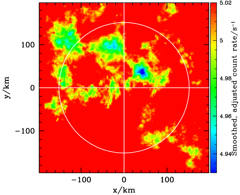
Figure 11: LEND CSETN smoothed count rate map of the lunar south pole.

Figure 12: Fractional count rate difference as a function of distance from the south pole along longitude $45^{\circ}$, through Shoemaker crater. The filled circles and crosses show results for the LPNS and LEND CSETN respectively. Each data point corresponds to one of the $10$ km pixels along $y=x$ in Figures 4 and 5. A uniform background of $f_{\rm b}=0.54$ has been removed to enhance the contrast in the LEND CSETN map. Error bars show the $1\sigma$ error on the mean $\delta$ in each pixel. The LEND CSETN results have been displaced by $2$ km in polar distance for clarity. Vertical dotted lines delineate the limits of Shoemaker crater.

Figure 13: Fractional count rate difference as a function of longitude for a $10$ km-wide annulus at latitude $-88^{\circ}$. Filled circles and crosses show results for the LPNS and LEND CSETN respectively. Data points every $\sim 10$ km in azimuth are shown and a uniform background of $f_{\rm b}=0.54$ has been removed to enhance the contrast in the LEND CSETN map. Error bars on the LEND CSETN points show the $1\sigma$ error on the mean $\delta$ in each pixel. For clarity, the relatively small uncertainties ($\sim\pm 0.01$) on the LPNS results are not shown. Vertical dotted lines delineate the limits of Shoemaker crater.

4.3 The lunar uncollimated background

In order to produce maps of the collimated lunar component, Boynton et al. (2012), Sanin et al. (2012) and Mitrofanov et al. (2012) remove a component of uncollimated lunar background flux from the LEND CSETN count rate. Despite the choice of colour scheme, figure 9 of Boynton et al. (2012) shows that the range of variation in combined background from the spacecraft and lunar uncollimated components amounts to no more than $\sim 4$ parts in $1000$. This means that it is essentially spatially invariant near the pole, and any fluctuations seen in the total count rate map are ascribed to the lunar collimated component. This lack of variation in the lunar uncollimated component at the poles is inconsistent with that predicted by Monte Carlo neutron transport models (Lawrence et al., 2011). Furthermore, the low value of $1.1$ counts per second assumed by Boynton et al. (2012) for the lunar uncollimated component would not be able to recreate the higher count rates seen over mare regions by the LEND CSETN (Lawrence et al., 2011; Eke et al., 2012).

Mitrofanov et al. (2012) adopt a slightly different approach that has a very similar effect. A “reference” map is made by smoothing the LEND CSETN data on a scale of $\sim 230$ km. The difference between this greatly smoothed map and one with a latitude-dependent smoothing radius of $11$ km at the pole growing to $25$ km at $-70^{\circ}$ latitude is used to determine where “local suppression/excess spots” exist. If the lunar uncollimated background results from neutrons coming from a scale of $\sim 80$ km across on the lunar surface, as one might anticipate for an omni-directional detector at an altitude of $50$ km, then this reference map will be too smooth to include any regional variations due to uncollimated lunar flux. Any such variations will then be ascribed to the collimated lunar component, which is anyway already smoothed on scales larger than the collimator field of view. There is no way that such an analysis can determine whether or not the LEND CSETN is behaving as a collimated detector.

Sanin et al. (2012) define their “local background” for a given crater using either a region at the same latitude or the LEND CSETN polar map smoothed on a similar large scale to Mitrofanov et al. (2011). The similarity between figure 1 in Sanin et al. (2012) and figure 1 in Mitrofanov et al. (2012) suggests that the same latitude-dependent smoothing of the map has been used in order to suppress noise on smaller scales. Sanin et al. (2012) conclude that there are three large permanently shaded regions (PSRs) that contain significant neutron suppressions, while smaller PSRs do not contain significant deviations from the background count rate. No effort is made to compare these measured neutron suppressions, which seem completely in keeping with what one would expect if little of the count rate was actually collimated, with what would be found with the LPNS. As pointed out in section 4.1, a count rate dip above Shoemaker crater is also very well detected by the LPNS. Thus, no substantive evidence to support claims about the functioning of the collimator in the LEND CSETN can be drawn from the paper by Sanin et al. (2012).

4.4 Orbital Phase Profiles

Litvak et al. (2012a) use the orbital phase profile to conclude that the collimated count rate into the LEND CSETN is $1.7$ neutrons per second. The orbital phase profile involves averaging over narrow latitude bands either on the near or far side of the Moon. The lengths of these bands are very much greater than the field of view of the collimator, so the purpose of the orbital phase profile is to compare large-scale features in global maps of different energy neutrons in order to determine the fractions of the total LEND CSETN count rate in the lunar collimated and lunar uncollimated components. To achieve this aim, Litvak et al. (2012a) assume that the lunar uncollimated component has a variation with longitude and latitude that matches that of the fast neutrons measured by the LEND Sensor for High Energy Neutrons (SHEN). Not only is this assumption unjustified, but it is also unjustifiable. Monte Carlo neutron transport simulations by Lawrence et al. (2011) suggest that high energy epithermal (HEE) neutrons are the primary contributor to the uncollimated lunar count rate, with a smaller portion from fast neutrons. This is important because, while both HEE and fast neutron fluxes are similarly changed by the increase in mean atomic mass in the mare regions, the HEE neutrons are much more sensitive to hydrogen near the lunar poles. Thus, the assumption made by Litvak et al. (2012a) forces the large-scale polar count rate dips to be ascribed to a significant collimated component because the variation of the uncollimated component has been falsely denied the opportunity to contribute to these polar count rate dips. Had the altitude dependence of the count rate variation been simultaneously investigated, then the inappropriateness of this assumption would have been evident.

5 Discussion

The results of the autocorrelation function and power spectrum analyses contained in this paper indisputably show how, even in the polar regions, the maps from the LEND CSETN are lower contrast than those from the LPNS on a range of scales. While much of this is due to the dominant, spatially invariant spacecraft-generated neutron background into the LEND CSETN, the lunar component of the count rate is also seen to display less small-scale power than is found by the LPNS. This deficit of small-scale structure exists to such an extent that the LEND CSETN results are best described by a model where the detector footprint is even slightly broader than omni-directional for a spacecraft at the $50$ km altitude of LRO. The $10$ km spatial resolution claimed by some authors (Mitrofanov et al., 2010, 2011, 2012; Boynton et al., 2012) is inconsistent with the LEND CSETN data themselves, and thus, once again, this should be rejected as a viable hypothesis. Further, claims that hydrogen enhancements are not co-located with permanently shaded regions (Mitrofanov et al., 2010) and that hydrogen enhancements are equally likely in shaded and sunlit regions (Mitrofanov et al., 2012) are not supported by the LEND CSETN data.

With just a straightforward scaling argument, one can see why the LPNS produces a more significant map of the count rate variations and hence hydrogen distribution. Suppose that the neutron count rate measured for regolith containing no hydrogen, $s_{0}$, were precisely known for both the LPNS and the LEND CSETN. The ratio of lunar neutron count rate, $s$, to $s_{0}$ sets the local hydrogen abundance. How much longer would the LEND CSETN need to collect data to receive the same accuracy in the derived hydrogen abundance as the LPNS, assuming that they actually have the same sized footprint? If there were not a large spacecraft background contribution to the LEND CSETN, then it would receive just $\sim 2$ neutrons per second, which is about a tenth of the LPNS rate. Thus it would need an observation period ten times as long as that of the LPNS to determine $s/s_{0}$ to the same fractional precision. However, the uniform spacecraft background contains a comparable variance to that in the lunar signal itself and the background and spacecraft neutrons are not distinguishable for the LEND CSETN. This means that, assuming the mean background count rate were precisely known, an extra factor of two in integration time is required to recover the same fractional accuracy in the inferred hydrogen abundance. Consequently, for the LEND CSETN to match the hydrogen map from 7 months of the LPNS at an altitude of $30$ km would require $t_{\rm LEND}\sim 20~{}t_{\rm LP}\sim 12$ years. Even then, the LEND CSETN map would be lower spatial resolution because of the broader instrumental footprint.

At the lower orbital altitude of $30$ km, the omni-directional LPNS map already contains more significant structure than is present in that from the LEND CSETN. Furthermore, the application of image reconstruction techniques has been shown to enhance the contrast in the count rate map by suppressing the inevitable stochastic noise and undoing some of the blurring that is unavoidably associated with the extended detector footprint. This objective assessment makes clear that the most accurate maps of the lunar polar hydrogen distribution are those resulting from LPNS data processed through an image reconstruction algorithm.

The arguments put forward by Mitrofanov et al. (2011); Litvak et al. (2012a, b) and Boynton et al. (2012) in support of the LEND CSETN functioning well as a collimated neutron detector have been considered in the previous section. None of them are found to provide strong evidence to bolster the claims that the majority of the lunar component into the LEND CSETN is collimated. Their conclusions appear to result from a mixture of unjustifiable or demonstrably incorrect assumptions, a misapplication of statistics, or an unrepeatable data reduction process. In contrast, the wide range of measurements considered in detail in this paper are all consistent with the component fractions inferred by Eke et al. (2012); namely that the uniform spacecraft background produces just over half of the counts into the LEND CSETN, with the spatially varying uncollimated lunar background close behind and the collimated lunar component providing fewer than $5\%$ of the total counts.

Collimating epithermal neutrons is distinctly non-trivial and the claims that the LEND CSETN is producing maps with a spatial resolution of $10$ km are extraordinary. “In science, the burden of proof falls upon the claimant; and the more extraordinary a claim, the heavier is the burden of proof demanded” (Truzzi, 1987). However, many lines of evidence reject the hypothesis that this level of spatial resolution is achieved. An alternative hypothesis, consistent with the available evidence, was provided by Eke et al. (2012). This hypothesis has passed the further testing performed in this paper, where the different techniques employed have further quantified the footprint of the LEND CSETN. It is likely that plans for future missions to the lunar poles will use maps of the hydrogen distribution, so it is important that the capabilities of the LEND CSETN are properly appreciated in order to prevent costly future mistakes in targetting landers.

Given that the performance of the LEND CSETN instrument has been shown here to be greatly inconsistent with the claims made by various authors, and has not met its primary objective of mapping the lunar neutron flux at a spatial resolution of $\sim 10$ km, one might reasonably ask how these data can best be used. The detector has, as was pointed out by Eke et al. (2012), made the first map of lunar neutrons with this particular energy-dependent filter that is picking out a mixture of high energy epithermal and fast neutrons. While the map is noisy and suffers from both a large spacecraft background and a very extended spatial footprint, it is still a unique resource. In order to extract scientifically useful results from this instrument, the challenge will be to understand the neutron transport within LRO well enough to determine which energies of neutron is the LEND CSETN measuring, and what they reveal about the composition of the lunar surface.

6 Conclusions

The best available maps of polar hydrogen come from the pixon reconstructions of LP data. These provide estimates of the average weight percentage of water equivalent hydrogen in polar craters that range up to a few per cent and have a fractional uncertainty of $\sim 30\%$ (Teodoro et al., 2010). The LEND CSETN produces maps containing a dominant background from neutrons that arise due to cosmic ray interactions with the spacecraft. The effective detector footprint, taking into account both the collimated lunar and uncollimated background lunar counts may even be broader than that for an omni-directional detector at $50$ km altitude. The suppression in the count rate over Shoemaker crater is consistent with a statistical fluctuation superimposed upon a broad dip in count rate of the sort that an omni-directional detector such as the LEND CSETN would measure in this region. Thus, it does not support the claim that the LEND CSETN is collimated.

The results of this study are relevant to the proposed “Fine Resolution” Epithermal Neutron Detector (Malakhov et al., 2012, FREND) that is scheduled to be launched in 2016 on the ExoMars mission.

References

- Arnold [1979] Arnold, J. R., Ice in the lunar polar regions, J. Geophys. Res., 84, 5659–5668, 1979.
- Boynton et al. [2012] Boynton, W. V., et al., High spatial resolution studies of epithermal neutron emission from the lunar poles: Constraints on hydrogen mobility, Journal of Geophysical Research (Planets), 117, E00H33, 10.1029/2011JE003979, 2012.
- Chin et al. [2007] Chin, G., et al., Lunar Reconnaissance Orbiter Overview: The Instrument Suite and Mission, Space Sci. Rev., 129, 391–419, 10.1007/s11214-007-9153-y, 2007.
- Christensen-Dalsgaard et al. [1985] Christensen-Dalsgaard, J., D. Gough, and J. Toomre, Seismology of the sun, Science, 229, 923–931, 10.1126/science.229.4717.923, 1985.
- Colaprete et al. [2010] Colaprete, A., et al., Detection of Water in the LCROSS Ejecta Plume, Science, 330, 463–, 10.1126/science.1186986, 2010.
- Cole et al. [2005] Cole, S., W. J. Percival, J. A. Peacock, and P. Norberg, The 2dF Galaxy Redshift Survey: power-spectrum analysis of the final data set and cosmological implications, Mon. Not. R. Astron. Soc., 362, 505–534, 10.1111/j.1365-2966.2005.09318.x, 2005.
- Eisenstein et al. [2005] Eisenstein, D. J., I. Zehavi, D. W. Hogg, R. Scoccimarro, M. R. Blanton, R. C. Nichol, and R. Scranton, Detection of the Baryon Acoustic Peak in the Large-Scale Correlation Function of SDSS Luminous Red Galaxies, ApJ, 633, 560–574, 10.1086/466512, 2005.
- Eke [2001] Eke, V., A speedy pixon image reconstruction algorithm, Mon. Not. R. Astron. Soc., 324, 108–118, 10.1046/j.1365-8711.2001.04253.x, 2001.
- Eke et al. [2009] Eke, V. R., L. F. A. Teodoro, and R. C. Elphic, The spatial distribution of polar hydrogen deposits on the Moon, Icarus, 200, 12–18, 10.1016/j.icarus.2008.10.013, 2009.
- Eke et al. [2012] Eke, V. R., L. F. A. Teodoro, D. J. Lawrence, R. C. Elphic, and W. C. Feldman, A Quantitative Comparison of Lunar Orbital Neutron Data, ApJ, 747, 6, 10.1088/0004-637X/747/1/6, 2012.
- Elphic et al. [1998] Elphic, R. C., D. J. Lawrence, W. C. Feldman, B. L. Barraclough, S. Maurice, A. B. Binder, and P. G. Lucey, Lunar Fe and Ti Abundances: Comparison of Lunar Prospector and Clementine Data, Science, 281, 1493, 10.1126/science.281.5382.1493, 1998.
- Elphic et al. [2007] Elphic, R. C., V. R. Eke, L. F. A. Teodoro, D. J. Lawrence, and D. B. J. Bussey, Models of the distribution and abundance of hydrogen at the lunar south pole, Geophys. Res. Lett., 34, L13,204, 10.1029/2007GL029954, 2007.
- Feldman et al. [1991] Feldman, W. C., R. C. Reedy, and D. S. McKay, Lunar neutron leakage fluxes as a function of composition and hydrogen content, Geophys. Res. Lett., 18, 2157–2160, 10.1029/91GL02618, 1991.
- Feldman et al. [1998a] Feldman, W. C., B. L. Barraclough, S. Maurice, R. C. Elphic, D. J. Lawrence, D. R. Thomsen, and A. B. Binder, Major Compositional Units of the Moon: Lunar Prospector Thermal and Fast Neutrons, Science, 281, 1489, 10.1126/science.281.5382.1489, 1998a.
- Feldman et al. [1998b] Feldman, W. C., S. Maurice, A. B. Binder, B. L. Barraclough, R. C. Elphic, and D. J. Lawrence, Fluxes of Fast and Epithermal Neutrons from Lunar Prospector: Evidence for Water Ice at the Lunar Poles, Science, 281, 1496–1500, 1998b.
- Feldman et al. [2000] Feldman, W. C., D. J. Lawrence, R. C. Elphic, B. L. Barraclough, S. Maurice, I. Genetay, and A. B. Binder, Polar hydrogen deposits on the Moon, J. Geophys. Res., 105, 4175–4196, 10.1029/1999JE001129, 2000.
- Gasnault et al. [2001] Gasnault, O., W. C. Feldman, S. Maurice, I. Genetay, C. d’Uston, T. H. Prettyman, and K. R. Moore, Composition from fast neutrons: Application to the Moon, Geophys. Res. Lett., 28, 3797-3800, 10.1029/2001GL013072, 2001.
- Lawrence et al. [2006] Lawrence, D. J., W. C. Feldman, R. C. Elphic, J. J. Hagerty, S. Maurice, G. W. McKinney, and T. H. Prettyman, Improved modeling of Lunar Prospector neutron spectrometer data: Implications for hydrogen deposits at the lunar poles, Journal of Geophysical Research (Planets), 111(E10), E08,001, 10.1029/2005JE002637, 2006.
- Lawrence et al. [2010] Lawrence, D. J., R. C. Elphic, W. C. Feldman, H. O. Funsten, and T. H. Prettyman, Performance of Orbital Neutron Instruments for Spatially Resolved Hydrogen Measurements of Airless Planetary Bodies, Astrobiology, 10, 183–200, 10.1089/ast.2009.0401, 2010.
- Lawrence et al. [2011] Lawrence, D. J., V. R. Eke, R. C. Elphic, W. C. Feldman, H. O. Funsten, T. H. Prettyman, and L. F. A. Teodoro, Technical Comment on ”Hydrogen Mapping of the Lunar South Pole Using the LRO Neutron Detector Experiment LEND”, Science, 334, 1058, 10.1126/science.1203341, 2011.
- Lawrence et al. [2013] Lawrence, D. J., et al., Evidence for Water Ice Near Mercury’s North Pole from MESSENGER Neutron Spectrometer Measurements, Science, 339, 292–, 10.1126/science.1229953, 2013.
- Lingenfelter et al. [1961] Lingenfelter, R. E., E. H. Canfield, and W. N. Hess, The Lunar Neutron Flux, J. Geophys. Res., 66, 2665–2671, 10.1029/JZ066i009p02665, 1961.
- Litvak et al. [2012a] Litvak, M. L., I. G. Mitrofanov, A. Sanin, A. Malakhov, W. V. Boynton, G. Chin, and G. Droege, Global maps of lunar neutron fluxes from the LEND instrument, Journal of Geophysical Research (Planets), 117, E00H22, 10.1029/2011JE003949, 2012a.
- Litvak et al. [2012b] Litvak, M. L., et al., LEND neutron data processing for the mapping of the Moon, Journal of Geophysical Research (Planets), 117, E00H32, 10.1029/2011JE004035, 2012b.
- Malakhov et al. [2012] Malakhov, A., et al., Fine Resolution Epithermal Neutron Detector (FREND) for ExoMarsTrace Gas Orbiter, in EGU General Assembly Conference Abstracts, EGU General Assembly Conference Abstracts, vol. 14, edited by A. Abbasi and N. Giesen, p. 9118, 2012.
- Maurice et al. [2004] Maurice, S., D. J. Lawrence, W. C. Feldman, R. C. Elphic, and O. Gasnault, Reduction of neutron data from Lunar Prospector, Journal of Geophysical Research (Planets), 109(E18), E07S04, 10.1029/2003JE002208, 2004.
- McHardy et al. [2006] McHardy, I. M., E. Koerding, C. Knigge, P. Uttley, and R. P. Fender, Active galactic nuclei as scaled-up Galactic black holes, Nature, 444, 730–732, 10.1038/nature05389, 2006.
- Metzger and Drake [1990] Metzger, A. E., and D. M. Drake, Identification of lunar rock types and search for polar ice by gamma ray spectroscopy, J. Geophys. Res., 95, 449–460, 10.1029/JB095iB01p00449, 1990.
- Mitrofanov et al. [2011] Mitrofanov, I., W. Boynton, M. Litvak, A. Sanin, and R. Starr, Response to Comment on ”Hydrogen Mapping of the Lunar South Pole Using the LRO Neutron Detector Experiment LEND”, Science, 334, 1058, 10.1126/science.1203341, 2011.
- Mitrofanov et al. [2012] Mitrofanov, I., M. Litvak, A. Sanin, A. Malakhov, D. Golovin, W. Boynton, G. Droege, and G. Chin, Testing polar spots of water-rich permafrost on the Moon: LEND observations onboard LRO, Journal of Geophysical Research (Planets), 117, E00H27, 10.1029/2011JE003956, 2012.
- Mitrofanov et al. [2008] Mitrofanov, I. G., A. B. Sanin, D. V. Golovin, M. L. Litvak, A. A. Konovalov, and A. A. Kozyrev, Experiment LEND of the NASA Lunar Reconnaissance Orbiter for High-Resolution Mapping of Neutron Emission of the Moon, Astrobiology, 8, 793–804, 10.1089/ast.2007.0158, 2008.
- Mitrofanov et al. [2010] Mitrofanov, I. G., A. B. Sanin, W. V. Boynton, G. Chin, J. B. Garvin, D. Golovin, and L. G. Evans, Hydrogen Mapping of the Lunar South Pole Using the LRO Neutron Detector Experiment LEND, Science, 330, 483–, 10.1126/science.1185696, 2010.
- Monin et al. [2007] Monin, A., A. Yaglom, and J. Lumley, Statistical Fluid Mechanics, Volume 1: Mechanics of Turbulence, Dover Books on Physics Series, Dover, 2007.
- Narteau et al. [2009] Narteau, C., D. Zhang, O. Rozier, and P. Claudin, Setting the length and time scales of a cellular automaton dune model from the analysis of superimposed bed forms, Journal of Geophysical Research (Earth Surface), 114, F03006, 10.1029/2008JF001127, 2009.
- Neumann et al. [2013] Neumann, G. A., et al., Bright and Dark Polar Deposits on Mercury: Evidence for Surface Volatiles, Science, 339, 296–, 10.1126/science.1229764, 2013.
- Paige et al. [2013] Paige, D. A., et al., Thermal Stability of Volatiles in the North Polar Region of Mercury, Science, 339, 300–, 10.1126/science.1231106, 2013.
- Peebles [1980] Peebles, P. J. E., The large-scale structure of the universe, Princeton University Press, 1980.
- Pina and Puetter [1993] Pina, R. K., and R. C. Puetter, Bayesian image reconstruction - The pixon and optimal image modeling, Publ. Astron. Soc. Pac., 105, 630–637, 1993.
- Planck Collaboration [2013] Planck Collaboration, Planck 2013 results. XV. CMB power spectra and likelihood, ArXiv e-prints, 2013.
- Sanin et al. [2012] Sanin, A. B., I. G. Mitrofanov, M. L. Litvak, A. Malakhov, W. V. Boynton, G. Chin, and G. Droege, Testing lunar permanently shadowed regions for water ice: LEND results from LRO, Journal of Geophysical Research (Planets), 117, E00H26, 10.1029/2011JE003971, 2012.
- Teodoro et al. [2010] Teodoro, L. F. A., V. R. Eke, and R. C. Elphic, Spatial distribution of lunar polar hydrogen deposits after KAGUYA (SELENE), Geophys. Res. Lett., 37, L12201, 10.1029/2010GL042889, 2010.
- Truzzi [1987] Truzzi, M., On Pseudo-Skepticism, Zetetic Scholar, 12/13, 3–, 1987.
- Watson et al. [1961] Watson, K., B. Murray, and H. Brown, On the Possible Presence of Ice on the Moon, J. Geophys. Res., 66, 1598–1600, 1961.
- Wieczorek and Phillips [1998] Wieczorek, M. A., and R. J. Phillips, Potential anomalies on a sphere - Applications to the thickness of the lunar crust, J. Geophys. Res., 103, 1715, 10.1029/97JE03136, 1998.