Estimating the properties of hard X-ray solar flares by constraining model parameters

Abstract

We wish to better constrain the properties of solar flares by exploring how parameterized models of solar flares interact with uncertainty estimation methods. We compare four different methods of calculating uncertainty estimates in fitting parameterized models to Ramaty High Energy Solar Spectroscopic Imager (RHESSI) X-ray spectra, considering only statistical sources of error. Three of the four methods are based on estimating the scale-size of the minimum in a hypersurface formed by the weighted sum of the squares of the differences between the model fit and the data as a function of the fit parameters, and are implemented as commonly practiced. The fourth method is also based on the difference between the data and the model, but instead uses Bayesian data analysis and Markov chain Monte Carlo (MCMC) techniques to calculate an uncertainty estimate. Two flare spectra are modeled: one from the GOES (Geostationary Operational Environmental Satellite) X1.3 class flare of 19 January 2005, and the other from the X4.8 flare of 23 July 2002. We find that the four methods give approximately the same uncertainty estimates for the 19 January 2005 spectral fit parameters, but lead to very different uncertainty estimates for the 23 July 2002 spectral fit. This is because each method implements different analyses of the hypersurface, yielding method-dependent results that can differ greatly depending on the shape of the hypersurface. The hypersurface arising from the 19 January 2005 analysis is consistent with a Normal distribution; therefore, the assumptions behind the three non-Bayesian uncertainty estimation methods are satisfied and similar estimates are found. The 23 July 2002 analysis shows that the hypersurface is not consistent with a Normal distribution, indicating that the assumptions behind the three non-Bayesian uncertainty estimation methods are not satisfied, leading to differing estimates of the uncertainty. We find that the shape of the hypersurface is crucial in understanding the output from each uncertainty estimation technique, and that a crucial factor determining the shape of hypersurface is the location of the low-energy cutoff relative to energies where the thermal emission dominates. The Bayesian/MCMC approach also allows us to provide detailed information on probable values of the low-energy cutoff, $E_{c}$, a crucial parameter in defining the energy content of the flare-accelerated electrons. We show that for the 23 July 2002 flare data, there is a 95% probability that $E_{c}$ lies below approximately 40 keV, and a 68% probability that it lies in the range 7–36 keV. Further, the low-energy cutoff is more likely to be in the range 25-35 keV than in any other 10 keV wide energy range. The low-energy cutoff for the 19 January 2005 flare is more tightly constrained to $107\pm 4$ keV with 68% probability. Using the Bayesian/MCMC approach, we also estimate for the first time probability density functions for the total number of flare accelerated electrons and the energy they carry for each flare studied. For the 23 July 2002 event, these probability density functions are asymmetric with long tails orders of magnitude higher than the most probable value, caused by the poorly constrained value of the low-energy cutoff. The most probable electron power is estimated at $10^{28.1}\mbox{erg sec}^{-1}$, with a 68% credible interval estimated at $10^{28.1-29.0}\mbox{erg sec}^{-1}$, and a 95% credible interval estimated at $10^{28.0-30.2}\mbox{erg sec}^{-1}$. For the 19 January 2005 flare spectrum, the probability density functions for the total number of flare accelerated electrons and their energy are much more symmetric and narrow: the most probable electron power is estimated at $10^{27.66\pm 0.01}\mbox{erg sec}^{-1}$ (68% credible intervals). However in this case the uncertainty due to systematic sources of error is estimated to dominate the uncertainty due to statistical sources of error.

1 Introduction

The detailed understanding of solar flares requires an understanding of the physics of accelerated electrons, since electrons carry a large fraction of the total energy released in a flare (Lin & Hudson, 1971, 1976; Emslie et al., 2004, 2005). Since we cannot measure the electron flux in situ, the behavior of the flare-accelerated electrons is inferred from the photons emitted by their interaction with the ambient plasma. For a general inhomogeneous optically thin source of plasma density $n(\mathbf{r})$ and electron flux density energy spectrum $F(E,\mathbf{r})$ (electrons $\mbox{cm}^{-2}\mbox{s}^{-1}\mbox{keV}^{-1}$) in volume $V$ for electron energy $E$, the bremsstrahlung photon flux density energy spectrum $I(\epsilon)$ (photons $\mbox{cm}^{-2}\mbox{s}^{-1}\mbox{keV}^{-1}$ at Earth distance $R$) can be written (Brown, 1971; Brown et al., 2003) as

$$I(\epsilon)=\frac{\overline{n}V}{4\pi R^{2}}\int_{\epsilon}^{\infty}\overline{F}(E)Q(\epsilon,E)dE,$$ (1)

where $\overline{n}=\int_{V}ndV/V$, $\overline{F}(E)$ is the mean electron flux distribution, $\overline{F}(E)=\int_{V}n(\mathbf{r})F(E,\mathbf{r})dV/(\overline{n}V)$, and $Q(\epsilon,E)$ is the bremsstrahlung cross-section differential in photon energy $\epsilon$. In this paper we model the photon flux density energy spectrum as the sum of emission due to a flare-injected electron flux spectrum interacting with a target, and emission from hot plasma with a Maxwellian distribution of speeds corresponding to some temperature $T$.

The Ramaty High Energy Solar Spectroscopic Imager (RHESSI, Lin et al. 2002) flags all photons detected in any one of the nine germanium detectors by the time of occurrence (to 1 microsecond), the amount of energy lost by the photon in the detector (in 0.3-keV-wide pulse height analyzer (PHA) bins), and the detector number. For spatially integrated spectral analysis, the counts can be combined arbitrarily over different detectors and PHA bins.

We define $\mathbf{D}$= $(D_{1},...,D_{i},...D_{n})$ as the number of counts observed in a given set of energy-loss bins labeled in the range $1\leq i\leq n$ in a given time interval. These counts are noisy, and are assumed to be drawn from a Poisson distribution with a mean of $C_{i}$,

$$p(D_{i})=\frac{C_{i}^{D_{i}}}{D_{i}!}e^{-C_{i}}.$$ (2)

The measured count rate $R^{D}_{i}$ in energy-loss bin ‘$i$’ is determined from the measured counts $D_{i}$ divided by the live time $t_{LT}$. The predicted count rate $R^{C}_{i}$ arises from the incident photon flux rate via

$$R^{C}_{i}=M_{ij}I_{j};$$ (3)

that is, the predicted count rate in an energy-loss bin ‘$i$’ is modeled via a detector response matrix $M_{ij}$ for an incident photon flux spectrum $I_{j}$, where the index $j$, $1\leq j\leq m$, labels energies at which the incident photon spectrum is calculated. The response matrix $M_{ij}$ is calculated by RHESSI Solarsoft routines once the count energy-loss bins (indexed by ‘$i$’) and incident photon energies (indexed by ‘$j$’) are defined. The incident photon flux energy spectrum is deduced by comparing the observed with the predicted count rates in all energy bins assuming a model for the photon flux energy spectrum until some criterion for agreement is met.

One goal of RHESSI data analysis is to recover the electron flux energy spectrum $F(E,\mathbf{r})$ from the detected counts $D_{i}$ in a given time interval. In general, this requires detailed knowledge of the energy losses suffered by the bremsstrahlung-producing electrons in the emitting volume. It is often only practical to recover $\overline{F}(E)$; to do this, two approaches are commonly taken.

Since the rates are measured, and everything other than $\overline{F}(E)$ is known (either calculated, measured or assumed), $\overline{F}(E)$ can be obtained through Equations 1 and 3. This approach is known as inversion. The advantage of inversion is that one does not make an assumption as to the nature of the mean electron flux distribution. The disadvantage of this approach is that noise in the observed data and errors in instrument calibration can lead to the creation of spurious features in the solution. This effect can be mitigated by adding extra constraints to the inversion process which forces the solution to be smooth across energy bins (note that this is required by the bremsstrahlung process and RHESSI’s energy resolution). Consider discretizing Equation 1 by energy bins to yield a matrix expression,

$$\mathbf{J}=\mathbf{A}\mathbf{F}$$ (4)

where $\mathbf{J}$ is a $m$-element vector representing the observed number of photons $I(\epsilon)$, $\mathbf{A}$ is a $m\times n$=matrix representing $Q(\epsilon,E)$ and $\mathbf{F}$ is a $n$-element vector representing the mean electron spectrum $\overline{F}(E)$. The standard approach is to minimize the residual

$$||\mathbf{A}\mathbf{F}-\mathbf{J}||$$

for $\mathbf{F}$ where $||\cdot||$ is the Euclidean norm. This matrix problem can be ill-posed due to the noise sources discussed above, or by $\mathbf{A}$ being ill-conditioned or singular. Regularization mitigates these issues by imposing extra constraints on the solution for $\mathbf{F}$. Tikhonov regularization does this by adding an extra term $||\mathbf{\Gamma}\mathbf{F}||$ for some choice of Tikhonov matrix $\mathbf{\Gamma}$, to the above minimization problem, yielding

$$\min_{\mathbf{F}}\left(\mathbf{|}|\mathbf{A}\mathbf{F}-\mathbf{J}||+||\mathbf{\Gamma}\mathbf{F}||\right).$$ (5)

Piana et al. (2003) demonstrate a Tikhonov-regularized inversion algorithm that takes the observed counts and finds $\overline{F}(E)$ and the uncertainty on $\overline{F}(E)$. Piana et al. (2003) show that this method led to an unexpected ‘dip’ in the mean electron spectrum which is thought (in most cases) to arise from the presence of a significant photospheric albedo flux contributing to the observed X-ray flux (Kontar et al., 2006, 2008).

In the second approach, known as forward fitting, a parameterized model for the mean electron flux distribution $\overline{F}(E)$ is used to describe the photon flux $I_{j}$ incident at RHESSI. The photon emission, parameterized by $\mathbf{\theta}$ ($N_{\mathbf{\theta}}$ variables) is

$$I_{j}=I_{j}(\mathbf{\theta}).$$ (6)

A fitting process is then used to find values of the parameters that best reproduce the counts $D_{i}$ observed by RHESSI. The disadvantage of this method is that the spectral model is prescribed rather than derived, and so features that are not in the model cannot be described by it, although their presence in the data may be indicated by the residuals (Brown et al., 2006). The advantages of this method are that by judicious choice of parameterization the major features of the spectrum can be modeled, and values to the parameters with uncertainty estimates can be obtained.

In this paper, we use the forward fitting approach and consider four different methods of estimating a range of “acceptable” model parameter values that describe our understanding of the flare within the confines of the model. By comparing different methods, we seek to understand the differences in the final answer that may be brought about by the way the estimates were obtained. Further, by comparing two different spectra we can better understand how, for a given model, the estimated parameter values and errors are influenced by the data. It is assumed that the only source of noise is the Poisson distribution that follows naturally from independent photon events (Eq. 2).

Systematic error sources are undoubtedly important in determining the uncertainties in the model parameters (Lee et al., 2011), but they are not explicitly included in the uncertainty determination methods described below. Two types of systematic uncertainties are common in this type of spectroscopy, integral and differential. Integral uncertainties are basically the uncertainties in the overall sensitivity of a given detector. Based on comparisons of flare spectra measured with different detectors, they are known to be smaller than approximately 10%. They affect primarily the absolute value of the emission measure in the thermal model and the total electron flux in the nonthermal electron spectrum. The differential uncertainties are basically the uncertainties in the sensitivity in each energy bin with respect to its neighbors. They affect primarily model parameters that depend on the slope of the measured spectrum. They are therefore important for the temperature in the thermal model and the low energy cutoff and power-law index of the nonthermal electron spectrum. For RHESSI, the differential uncertainties are less than 1% and are generally negligible compared to the statistical uncertainties. Milligan & Dennis (2009) (using detectors 1, 3, 4, 5, 6, and 9) and Su et al. (2011) (using detectors 1, 3, 4, 6, 8 and 9) show that there is scatter in the best-fit parameter values determined from different individual detectors for the flare models they considered but that the range of the scatter indicates that the systematic errors are not significantly greater than the statistical errors. The systematic uncertainties are not important in developing a basic understanding of how each uncertainty determination method behaves in the presence of noisy data and consequently they have not been included in the analysis done for this paper.

The observations and spectral models are described in Section 2. Section 3 describes the parameter and uncertainty estimation methods used. Section 4 describes the results and Section 5 discusses the implications of these results for fitting spectral models to RHESSI data.

2 Spectral model and observations

In the X-ray energy range covered by RHESSI (Lin et al., 2002) – generally from $\sim$3 keV up to a few hundred keV – the emitted photon spectrum is modeled as the sum of a thermal component that generally dominates at the lower X-ray energies, typically below $\sim$10–20 keV, and a non-thermal component that dominates at higher energies. The thermal component is the line and continuum emission from the flare-heated plasma. The line emission is mainly from transitions in highly ionized iron – primarily FeXXV – that appears in the RHESSI spectrum as an unresolved peak at 6.7 keV with a much weaker feature at $\sim$8 keV. The continuum emission is a combination of free-free emission (bremsstrahlung) and free-bound emission (recombination radiation).

For our spectral analysis, we have used the thermal line-plus-continuum spectra provided by CHIANTI (Dere et al., 1997, 2009) assuming an isothermal plasma with the ionization balance given by Mazzotta et al. (1998) and the “sun coronal” abundances given by Feldman et al. (1992). The only free parameters are the temperature ($kT$ in keV) and the volume emission measure ($EM$ in $cm^{-}3$).

The thermal continuum emission is made up of the sum of bremsstrahlung (or free-free) emission and free-bound emission. The form of the bremsstrahlung contribution as a function of photon energy $\epsilon$ is approximately

$$I_{thermal}(\epsilon)\propto\frac{[EM]}{\epsilon T^{1/2}}\exp(-\epsilon/kT),$$ (7)

where $k$ is Boltzmann’s constant and $I_{thermal}$ is in units of photons $s^{-1}\mbox{erg}^{-1}$ (Tandberg-Hanssen & Emslie, 1988). The free-bound continuum spectrum has a similar dependency on EM and T.

The non-thermal component of the measured X-ray spectrum is bremsstrahlung from flare-accelerated electrons interacting with the ambient medium. Following Brown (1971), we assume a cold, thick target, meaning that the electrons collisionally lose their energy in cold, fully ionized plasma as they radiate. The energy loss rate per unit distance $x$ as an electron with speed $v$ streams through the ambient plasma is $dE/dx=-2Kn_{e}(x)/(mv^{2})$, where $m$ is the electron mass, $n_{e}(x)$ is the number density of plasma electrons, and $K$ is approximately constant (see Holman et al., 2011). Using this result, the mean electron flux becomes

$$\overline{F}(E)={1\over\overline{n}V}\frac{mv^{2}}{2K}\int_{E}^{\infty}F_{0}(E_{0})dE_{0},$$ (8)

where $F_{0}(E_{0})$ is now the injected electron flux energy spectrum (electrons s^-1 keV^-1). We use the following broken power-law functional form for the spectrum of injected electrons:

$$F_{0}(E_{0})=A\left\{\begin{array}[]{ll}0&E_{0}<E_{c}\\ (E_{0}/E_{p})^{-\delta_{1}}&E_{c}\leq E_{0}<E_{b}\\ (E_{0}/E_{p})^{-\delta_{2}}(E_{b}/E_{p})^{\delta_{2}-\delta_{1}}&E_{b}\leq E_{0}<E_{h}\\ 0&E_{0}\geq E_{h}\\ \end{array}\right..$$ (9)

The seven parameters of this nonthermal component are the normalization parameter $A$, the low- and high-energy cutoffs, $E_{c}$ and $E_{h}$, the pivot energy $E_{p}$, the break energy $E_{b}$, and the power-law indices below and above the break energy, $\delta_{1}$ and $\delta_{2}$, respectively. The radiated X-ray spectrum is modeled as the sum of the isothermal component and Equation 1, where $\overline{F}(E)$ is given by Equations 8 and 9. The X-ray emission is assumed to be isotropic and, with this assumption, the contribution flux from photospheric albedo to the total incident X-ray at the instrument can be estimated (see Kontar et al., 2011).

We model RHESSI spectral data from two flares – the GOES class X1.3 flare on 19 January 2005 starting at 08:03 UT, and the X4.8 flare starting at 00:18 UT on 23 July 2002. We choose these flares because previous studies have shown that the low-energy cutoff - $E_{c}$ - is estimated to lie in very different portions of the spectrum. In the 23 July 2002 event, the low-energy cutoff of the flare-accelerated electrons is estimated to have an energy in the region where the observed hard X-ray emission is thermally dominated. This makes it difficult to place limits on the low-energy cutoff since it is difficult to determine the signal of the flare-accelerated electrons against the dominant thermal bremsstrahlung emission. Most flares are thought to have low-energy cutoffs close to or in the region where the emission is dominated by thermal bremsstrahlung. In contrast, Warmuth et al. (2009) studied the 19 January 2005 event, and found that late in the impulsive phase, the low-energy cutoff energy much higher than energies at which the thermal bremsstrahlung dominates. Therefore, thermal bremsstrahlung cannot be a significant factor in determining the uncertainty in the low-energy cutoff for this flare. The low-energy cutoff is one of the most important properties of a flare as its value strongly influences the estimated flare-accelerated electron energy content. Therefore, knowledge of the uncertainty in the low-energy cutoff directly influences knowledge of the energy content of the flare. Hence, these two flares and the models used to study them are good test-beds for understanding how different uncertainty estimation methods operate when generating uncertainties for parameters that are crucial for understanding the properties of solar flares.

Table 1 has details of the two flares and the two spectral accumulation times chosen, the models used, and the best-fit parameter values obtained that fit the spectral models to the data (see Section 3.1). These two spectra were chosen because they were both well observed with RHESSI and they highlight the excellent spectral capabilities of the cooled germanium detectors of this instrument (Smith et al., 2002). Both flares have been extensively analyzed previously – see for example Warmuth et al. (2009) for the 19 January 2005 flare and Holman et al. (2003) for the 23 July 2002 flare. The most notable difference between the two spectra is that the first has a low-energy cutoff in the electron spectrum of over 100 keV, well above the thermal component. This is in contrast to the second flare where the low-energy cutoff is estimated to be below $\sim$ 40 keV (Holman et al., 2003) and consequently difficult to determine because of the dominance of the thermal component at lower energies. This difference between these two flares motivates their selection for this study. These two flare events are good candidates that allow us to explore how well we can determine the value of the crucial low-energy cutoff parameter (and flare properties that depend on it) given the data, the model, and the uncertainty estimation methods used.

Traditionally, RHESSI spectral analysis involves summing data from multiple RHESSI detectors to improve counting statistics – see for example Su et al. (2009). Instead of this usual approach, we chose to use data from just one detector with good energy resolution and sensitivity – detector #4. This allowed us to apply the most accurate corrections for energy resolution and calibration, pulse pile-up, and background subtraction. In the time periods selected, the count rates were sufficiently high that selecting a single detector did not seriously degrade the spectroscopy capability up to the highest energies considered of $\sim$500 keV. The energy bin widths were chosen to be as narrow as possible to preserve spectral details resolvable with the detector’s $\sim$1 keV FWHM spectral resolution while maintaining $>$30 counts in each bin as required for the $\chi^{2}$ analysis procedure to be approximately valid Wasserman (2003). The only part of the spectral data that is affected by small numbers is at the high energy part of the spectrum, well away from the low energy part of the spectrum. At these energies, the simple Normal approximation to the Poisson distribution – ($Poisson(\lambda)\approx N(\lambda,\sqrt{\lambda})$ for $\lambda$ ’large’) – is no longer appropriate. However, the gross properties we are most interested in - flare energy content, the number of flare-accelerated electrons and the probability density function of the low-energy cutoff, are largely unaffected by a biassed fit of a spectral model to the data at high energies, since these properties are largely determined by the flare spectrum at energies where the Normal distribution can be used. We can assert this for the flares studied in this analysis because these are relatively large flares with large numbers of counts. The vast majority of flares are smaller than the ones studied here, and therefore fits or parameterized models to the data are more likely to suffer from biassed fits over more extensive energy ranges.

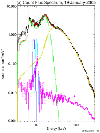
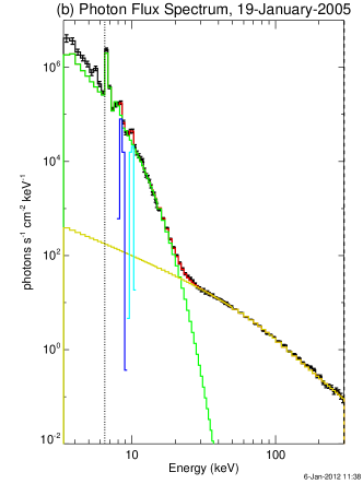
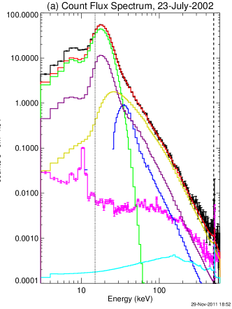
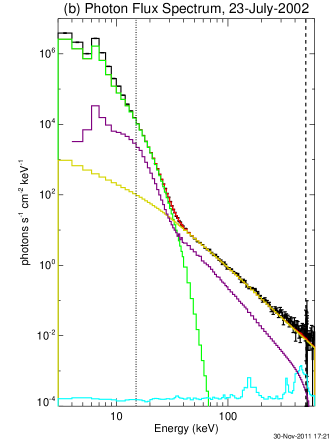
Both flares have been extensively analyzed previously –- see for example Warmuth et al. (2009) for the 19 January 2005 flare and Holman et al. (2003) for the 23 July 2002 flare. For ease in comparing results in each case, we have generally followed their lead in choosing background spectra, energy ranges, model components, fitting procedures, etc. in the spectral analysis. Table 1 has details of the two flares and the two spectral accumulation times chosen, the models used, and the best-fit parameter values obtained that fit the spectral models to the data (see Section 3.1). Corresponding count flux and photon flux spectra are shown in Figures 1 and 2. The model count flux spectrum is computed by taking the best fit photon spectrum and convolving it with the instrument response matrix. Figures 1b and 2b shows the best fit photon spectrum and the photon spectrum derived from the measured count flux spectrum using the ratio of the best fit photon spectrum to the measured counts in each energy bin. The units in Figures 1 and 2b are photons $s^{-1}cm^{-2}keV^{-1}$.)

2.1 19 January 2005

The first flare considered was the GOES X1.3 flare that peaked at 08:22 UT on 19 January 2005 on the solar disc at N15W51. We used the RHESSI observations of this flare from 08:26:00 - 08:26:20 UT, the same time interval when Warmuth et al. (2009) found an unusually hard spectrum during the final peak of the impulsive phase, possibly resulting from a low-energy cutoff in the electron spectrum as high as 120 keV (see their Figure 1 for RHESSI light-curves of this event).

We used the standard procedures that form OSPEX, the standard spectral analysis package used in RHESSI data analysis, to determine the best-fit parameters of the thermal and nonthermal components of the incident photon spectrum. As is common in RHESSI data analysis, the background spectrum that was subtracted from the measured count rate spectrum was calculated by linear interpolation in time between spectra measured before and after the flare. The estimated background spectrum is about an order of magnitude less than the flare spectrum at all energies considered. The background can therefore be considered as having very little influence on the final probability density functions of the model parameters and the gross properties of the flare such as its energy content and the number of flare accelerated electrons. Following Warmuth et al. (2009), we included two narrow Gaussian-shaped emission lines in the model photon spectrum to accommodate features in the count-rate spectra that are believed to be instrumental in origin.

We included the standard corrections for energy calibration adjustments and pulse pile-up, but these did not play a significant role for the selected time interval since the attenuators were in the A3 state (both thick and thin attenuators in place) resulting in relatively low counting rates. The albedo component was not included here, although it was included by Warmuth et al. (2009). We found that adding the albedo component did not significantly alter the fitted parameters or the estimates of the uncertainties. We used the following energy bins for this flare: $1/3$ keV from 3 to 15 keV, 1 keV from 15 to 50 keV, 5 keV from 50 to 100 keV, and 10 keV from 100 to 300 keV. The photon spectrum was extended above the fitted energy range up to 600 keV to allow for non-photopeak response of the detector.

Again, following Warmuth et al. (2009), we modeled the thermal component with a single-temperature function from CHIANTI using coronal abundances and a Mazzotta et al. (1998) ionization balance. The nonthermal component was modeled assuming thick-target interactions of electron with a single-power-law spectrum at energies above $E_{c}$. This is accommodated in Eq. 9 by fixing both $\delta_{2}$ at the default value of 6.0 and $E_{b}$ at 32 MeV so that they have no significant effect on the bremsstrahlung X-ray spectrum in the fitted photon energy range below 300 keV. $E_{h}$ was fixed at 32 MeV so that, like $E_{b}$, it has negligible effect on the bremsstrahlung X-ray spectrum in the fitted energy range, and so is equivalent to having no cutoff at all. For this flare, the normalization was taken to be $F_{0}$, the total integrated electron flux over the electron energy range from $E_{c}$ to $E_{h}$ with $E_{p}$ fixed at 1 keV, instead of $A$ in Eq. 9. The advantage in normalizing to $F_{0}$ is that this is a physically interesting quantity. The disadvantage is that it is strongly dependent on the value of both the low-energy cutoff and the spectral index. For the conditions described here, $F_{0}=AE_{c}^{1-\delta_{1}}/(\delta_{1}-1)$. The package OSPEX was configured to use this implementation of Equation 9 for this flare. An alternate implementation was required for the 23 July 2002 event (see Sections 2.2 and 4.2).

In our detailed spectral analysis and assessment of uncertainties, we had a total of seven free parameters – EM, kT, $F_{0}$, $E_{c}$, $\delta_{1}$, $G_{1}$ and $G_{2}$ – (see Table 1). Other parameters covering the instrumental effects - energy calibration, pulse pile-up, and Gaussian features below 10 keV - were determined from the analysis of the count-flux spectra for other time intervals and other flares, and then fixed for the subsequent determination of uncertainties in this time interval. The amplitudes of the two Gaussians ($G_{1}$ and $G_{2}$) were free during the spectral fits.

Figure 1: Count and photon spectra for the 19 January 2005 flare in the analysis period 08:26:00 to 08:26:20 UT. (a) The histograms with $\pm 1\sigma$ statistical error bars represent the background-subtracted count fluxes (black) and the background fluxes (pink) vs. energy loss in the detector. The smooth curves represent the different components of the model used to fit the data as follows: isothermal (green), thick-target bremsstrahlung (yellow), Gaussians (blue and cyan). The sum of all the components is shown in red. (b) Incident photon flux (in units of photons $s^{-1}cm^{-2}keV^{-1}$) vs. photon energy with the different components of the model shown in the same colors as in (a). The energy range used for the spectral fits lies between the vertical line at 6.45 keV and the edge of the plot at 300 keV.

2.2 23 July 2002

The second flare considered was the GOES X4.3 flare that peaked at 00:35 UT on 23 July 2002 from a location closer to the limb at S13E72 than the first event. Following Holman et al. (2003), we chose to analyze the time interval from 00:30:00 to 00:30:20.250 UT during the first peak of the impulsive phase (see their Figure 1 for RHESSI X-ray light-curves of this event; see also Lin et al. (2003), their Figure 1 for a lightcurve of the GOES X-ray flux). The measured X-ray spectrum was again assumed to be the sum of an isothermal spectrum and the thick-target bremsstrahlung spectrum from non-thermal electrons with the broken power-law of Eq. 9. In this case, the full double power-law was assumed with the break energy, $E_{b}$, and the second power-law index, $\delta_{2}$, both free parameters. The normalization constant for this flare, A in Eq. 9, was defined as the electron flux at the pivot energy $E_{p}$ that was fixed at 50 keV. As with the first flare, the high energy cutoff to the electron spectrum $E_{h}$ was set at 32 MeV to ensure that it had no significant effect in the fitted photon energy range.

The following 130 energy bins were used for this event: 1-keV wide bins from 3.0 to 40 keV, 3-keV from 40 to 100 keV, 5-keV bins from 100 to 150 keV, 10-keV bins from 150 to 500 keV, 1-keV bins from 501 to 520 keV, and 10-keV bins from 520 to 600 keV. We extended the energy range of the assumed photon spectrum up to 20 MeV to allow for the off-diagonal elements of the instrument response matrix due to the non-photopeak response of the detector. The fitted photon energy range was restricted to be above 15 keV to avoid the need for the two Gaussian emission line sources to accommodate the supposed instrumental features below 10 keV used for the first flare. The upper energy of the fit range was extended up to 500 keV to provide more information on the power-law spectrum above the break energy. This increase in the upper energy limit also necessitated adding in a nuclear component in the form of a template appropriate for a power-law ion spectrum (Murphy et al., 1991) with the normalization parameter fixed at the value obtained to give a best fit to the data. This nuclear component (shown in Fig. 2) contributes $<$10% to the photon flux at all energies below $\sim$400 keV and hence has only marginal significance in the subsequent analysis.

Other parameters were determined from least-squares fits to the count-flux spectrum and then fixed for the subsequent determination of uncertainties. These included parameters to characterize the instrumental effects of pulse pile-up that is a more important component for this flare since the count rates were a factor of $\sim$10 higher than in the first flare. Also, although it is not significant for flares at the solar limb, the albedo spectrum was included for this flare assuming isotropic X-ray emission using the the procedure described in Kontar et al. (2006) and implemented in OSPEX. Both the pile-up and albedo components are shown in Fig. 2.

For our detailed spectral analysis and assessment of uncertainties for this flare, there was a total of seven free parameters – EM, kT, A, $E_{c}$, $E_{b}$, $\delta_{1}$, $\delta_{2}$ (see Table 1). The background-subtracted count flux and photon spectra are shown in Fig. 2 along with the best-fit model components. Note that the implementation of the normalization used for this analysis is different from that used for the 19 January 2005 flare. In this analysis using the normalization $A$ at the pivot energy $E_{p}$ is preferred. The reason for this choice is given in Section 4.2.

Figure 2: Similar to Fig. 1 for the 23 July 2002 flare. The following three additional components are included in this plot: albedo (purple), pulse pile-up (blue), and the nuclear template (cyan). The two Gaussians shown in Fig. 1 were not used for this fit. The energy range used for the spectral fits lies between the two vertical lines at 15 and 500 keV.

Table 1: Flare characteristics and model parameters.

			Flare 1			Flare 2
Date			19 January 2005			23 July 2002
GOES Start/Peak/End Times			08:03/08:22/08:40 UT			00:18/00:35/00:47 UT
GOES Class			X1.3			X4.8
Location on the Sun			N15W51			S13E72
Radial distance from Sun center			763”			904”
Time Interval Analyzed			08:26:00 – 08:26:20 UT			00:30:00 – 00:30:20.250 UT
Fitted Photon Energy Range			6.45 to 300 keV			15 to 500 keV
Fitted Photon Energy Bins			90			90
	Parameter	Units	Value $\hat{\mathbf{\theta}}$	Free/Fixed		Value$\hat{\mathbf{\theta}}$	Free/Fixed
Thermal Plasma
	EM	$10^{49}$ cm-3	2.31	free		2.16	free
	Temp. (kT)	keV	2.03	free		3.18	free
	Abundance	coronal	1	fixed		1	fixed
Non-thermal Electrons
	$F_{0}$, integrated flux	$10^{35}$ s-1	0.17	free		not used
	$A$, flux  at $E_{p}$	$10^{35}$ s-1 keV-1	not used			0.028	free
	$E_{c}$	keV	105	free		32.0	free
	$E_{p}$	keV	1	fixed		50	fixed
	$E_{b}$	keV	32,000	fixed		256	free
	$E_{h}$	keV	32,000	fixed		32,000	fixed
	$\delta_{1}$		3.57	free		3.40	free
	$\delta_{2}$		6.0	fixed		3.92	free
Nuclear Template
	Normalization	photons cm-2	not used			2.11	fixed
Gaussians
	$G_{1}$ peak E	keV	8.44	fixed		not used
	$G_{2}$ peak E	keV	9.95	fixed		not used
	$G_{1}$ amplitude	photons cm-2 s-1	33,300	free		not used
	$G_{2}$ amplitude	photons cm-2 s-1	12,800	free		not used
	$G_{1,2}$ FWHM	keV	0.1	fixed		not used

3 Parameter and Uncertainty Estimation Methods

Four different methods of uncertainty estimation are described below. The first three methods - ‘covariance matrix’, ‘$\chi^{2}$-mapping’ and ‘Monte Carlo’ sampling (Sections 3.1.1, 3.1.2 and 3.1.3 respectively) are widely used to estimate errors in parameter values. The fourth method is based on Bayesian probability and the Markov chain Monte Carlo (MCMC) method (Section 3.2.1). Each of these methods is applied to the spectral model and data described in Section 2, and the results are tabulated in Table 2 (19 January 2005) and Table 3 (23 July 2002).

3.1 Methods 1-3: Parameter and uncertainty estimation via nonlinear least-squares fitting

The first three methods are based on finding a local minimum $\chi^{2}_{min}$ to the quantity

$$\chi^{2}=\sum_{i=1}^{n}\frac{[R^{D}_{i}-R^{C(\mathbf{\theta})}_{i}]^{2}}{w_{i}^{2}}.$$ (10)

for some value of $\mathbf{\theta}=\hat{\mathbf{\theta}}$ and $w_{i}$. The quantity $\chi^{2}$ is a hypersurface parameterized by $\mathbf{\theta}$. The quantity $\hat{\mathbf{\theta}}$ is found by performing a nonlinear weighted least squares fit minimizing $\chi^{2}$ with respect to $\mathbf{\theta}$. There are many different ways of implementing this minimization. The minimization was achieved using the OSPEX spectral analysis package which uses the IDL/Solarsoft routine MCURVEFIT.pro. This routine is based on the nonlinear least-squares Levenburg-Marquardt fitting algorithm of Press et al. (1992) (pages 675-683). This implementation of the algorithm ignores the second derivative of the fitting function $R^{C(\mathbf{\theta})}_{i}$ with respect to $\mathbf{\theta}$, and is therefore equivalent to assuming that the fitting function is linear with respect to $\mathbf{\theta}$ near the best-fit value $\hat{\mathbf{\theta}}$.

The value of $\hat{\mathbf{\theta}}$ is derived as follows. The process is begun with an initial estimate of $\hat{\mathbf{\theta}}$, $\mathbf{\theta}^{0}$. The corresponding flux rate spectrum $R^{C(\mathbf{\theta}^{0})}_{i}$ is calculated and $w_{i}$ is set to $\sqrt{C_{i}(\mathbf{\theta}^{0})}/t_{LT}$. This value of $w_{i}$ is passed to MCURVEFIT.pro. This routine refines the estimate of the values of the spectral parameters, stopping when the termination condition is met. This first estimate is to $\hat{\mathbf{\theta}}$ is labeled $\mathbf{\theta}^{1}$. The fitting routine is run again this time using $\mathbf{\theta}^{1}$ as the initial estimate to $\hat{\mathbf{\theta}}$ and with $w_{i}$ set to $\sqrt{C_{i}(\mathbf{\theta}^{1})}/t_{LT}$, yielding a second estimate $\mathbf{\theta}^{2}$. The routine is run a third and final time using $\mathbf{\theta}^{2}$ as the initial estimate to $\hat{\mathbf{\theta}}$ and with $w_{i}$ set to $\sqrt{C_{i}(\mathbf{\theta}^{2})}/t_{LT}$, yielding a final parameter estimate, labeled $\hat{\mathbf{\theta}}$.

Estimates of the uncertainty in the value $\hat{\mathbf{\theta}}$ are found by defining a scale-size of variation in the $\chi^{2}$-hypersurface around $\hat{\mathbf{\theta}}$ in different ways. Three different methods of defining and estimating the uncertainty in the value $\hat{\mathbf{\theta}}$ are described below.

3.1.1 Method 1: Uncertainty Estimation by Estimating the Covariance Matrix

This method uses the curvature matrix of the $\chi^{2}$-hypersurface evaluated at $\hat{\mathbf{\theta}}$ to estimate the uncertainty in each parameter, via the assumptions that the measurement errors in the data $\mathbf{D}$ are Normally distributed and that either the model $R^{C(\mathbf{\theta})}_{i}$ is linear in its parameters, or the region over which the uncertainty estimate spans can be replaced by a linear approximation to the original model.

The curvature matrix $\alpha$ of the the $\chi^{2}$-hypersurface arises in linear and nonlinear least-squares fitting algorithms and is defined as $\alpha_{ij}=\partial^{2}(\chi^{2})/(\partial\theta_{i}\partial\theta_{j})$ for $1\leq i,j\leq N_{\mathbf{\theta}}$. The implementation of MCURVEFIT.pro gives an uncertainty estimate to each of the free parameters based on the curvature matrix (Press et al., 1992). The uncertainty for $\hat{\theta_{i}}$ (for $1\leq i\leq N_{\mathbf{\theta}}$) is

$$\delta\theta_{i}=\pm\sqrt{{\alpha}^{-1}_{ii}},$$ (11)

when evaluated at $\mathbf{\theta}=\hat{\mathbf{\theta}}$ (the value that minimizes $\chi^{2}$, Equation 10). The quantity $\alpha^{-1}$ in the right-hand side of Equation 11 is the matrix inversion of the curvature matrix and is an estimate of the covariance matrix of the fit parameters, evaluated at $\hat{\mathbf{\theta}}$. Its diagonal elements are the covariance scale-sizes that defines the uncertainty estimates in this method. Full details of the derivation of Equation 11 are given in Press et al. (1992), pages 690–692. The assumptions in this derivation also imply that the probability distribution for $\delta\mathbf{\theta}_{obs}$ (the expected error in the value of $\hat{\mathbf{\theta}}$) is a multivariate Normal distribution around $\hat{\mathbf{\theta}}$. The uncertainty estimate given by Equation 11 is quoted as the 68% value in Tables 2 and 3.

3.1.2 Method 2: Uncertainty Estimation using $\chi^{2}$-mapping

In this method, parts of the shape of the $\chi^{2}$-hypersurface around $\chi^{2}_{min}$ are explicitly calculated. It is assumed that the value of the $\chi^{2}$-hypersurface as defined by Equation 10, at a particular point $\mathbf{\theta}$, follows a $\chi^{2}$-distribution. By fixing a probability and finding where that probability occurs as a function of the parameters, one can measure scale-sizes in the $\chi^{2}$-hypersurface that define an estimate of the uncertainty in the value of $\hat{\mathbf{\theta}}$ with that probability. The procedure is described below.

One of the parameters $\theta$ in the set $\mathbf{\theta}$ is stepped through a range of values while the others are allowed to vary so as to minimize $\chi^{2}$, yielding a value $\chi^{2}_{1}$. The quantity $\delta\chi^{2}=\chi^{2}_{1}-\chi^{2}_{min}$ is assumed to have a $\chi^{2}$-distribution with one degree of freedom (Press et al., 1992). For such a distribution one can therefore expect that $\delta\chi^{2}<1$ occurs approximately 68% of the time and $\delta\chi^{2}<4$ occurs approximately 95% of the time. Values for the 68% and 95% confidence intervals are found where

$$\delta\chi^{2}(\theta^{68\%})=1,\delta\chi^{2}(\theta^{95\%})=4,$$ (12)

respectively. The uncertainty estimates defined by this method are quoted as differences from $\hat{\mathbf{\theta}}$ in Tables 2 and 3, that is,

$$\theta^{100q\%}_{i}-\hat{\theta_{i}}$$ (13)

for $1\leq i\leq N_{\mathbf{\theta}}$ where $q=0.68$ and $q=0.95$ and $\theta^{100q\%}_{i}$ is defined by Equation 12. Typically there are two values of $\theta^{100q\%}_{i}$ that satisfy Equation 12 corresponding to the upper and lower confidence limits of the parameter value $\hat{\theta_{i}}$. When no value of $\theta$ can be found that satisfies the conditions of Equation 12, this is reported as ‘not determined’ in Tables 2 and 3. Finally, this method uses the same underlying assumptions as those in Section 3.1.1 (Press et al., 1992).

3.1.3 Method 3: Uncertainty Estimation using the Monte Carlo method

This method of obtaining uncertainty estimates on $\hat{\mathbf{\theta}}$ is commonly called the “Monte Carlo” method. This method begins by assuming that the value $\hat{\mathbf{\theta}}$ found in method 1 best describes the observation via the parameterized model. By Equation 3, this defines an estimated count flux rate spectrum of $R^{C(\hat{\mathbf{\theta}})}_{i}$ that is assumed to be a good estimate of the true count flux spectrum. Estimates of the errors in $\hat{\mathbf{\theta}}$ are found by generating a new spectrum such that counts in energy-loss bin i are drawn from a Poisson distribution with mean value $R^{C(\hat{\mathbf{\theta}})}_{i}$ for all $1\leq i\leq n$. This new spectrum is now fit using the same physical model and fit process as the original fit generating $\hat{\mathbf{\theta}}$. The sampling and fitting process is repeated; the distribution of values found is centered at $\hat{\mathbf{\theta}}$, and the width of distribution estimates the uncertainty in $\hat{\mathbf{\theta}}$. The sample and fit process is repeated 10,000 times, from which normalized frequency distributions $F(\theta_{i})$ $(1\leq i\leq N_{\mathbf{\theta}})$ are calculated. The uncertainty estimate used excludes the tail values in a frequency distribution $F(\theta_{i})$. The $100q$% uncertainty estimate for $0\leq q\leq 1$ is defined as $[\theta^{L}|_{q},\theta^{H}|_{q}]$ where

$$\int_{-\infty}^{\theta^{L}|_{q}}F(\theta_{i})d\theta_{i}=\int^{\infty}_{\theta^{H}|_{q}}F(\theta_{i})d\theta_{i}=(1-q)/2.$$ (14)

This definition finds an interval $[\theta^{L}|_{q},\theta^{H}|_{q}]$ such that $100q$% of the measurements are within the interval and an equal percentage of the measurements are both above and below the interval. This definition of the interval is also guaranteed to contain the median value (which can be found from Eq. 14 by setting $q=0$). The uncertainty estimates found by this method are quoted in Tables 2 and 3 as differences

$$\theta^{L}|_{q}-\hat{\theta_{i}},\theta^{H}|_{q}-\hat{\theta_{i}}$$ (15)

for $q=0.68$ and $q=0.95$ $(1\leq i\leq N_{\mathbf{\theta}})$.

3.2 Method 4: Parameter and uncertainty estimation using Bayesian data analysis

This method uses parameter and uncertainty estimation based on Bayesian data analysis methods (Jaynes, 2003; Gregory, 2005). In Bayesian data analysis, the probability of a hypothesis $H$ is calculated via Bayes’ theorem. Denoting by $p(a|b,c)$ the conditional probability that proposition $a$ is true given that propositions $b$ and $c$ are true, Bayes’ theorem is

$$p(H|\mbox{$\mathbf{D}$},\mathcal{I})=\frac{p(H|\mathcal{I})p(\mbox{$\mathbf{D}$}|H,\mathcal{I})}{p(\mbox{$\mathbf{D}$}|\mathcal{I})}$$ (16)

where $H$ is the hypothesis to be tested, $\mathbf{D}$ is the observation, and $\mathcal{I}$ is any other applicable information we have prior to calculating the posterior.

The left hand side $p(H|\mbox{$\mathbf{D}$},\mathcal{I})$ is called the posterior probability of the hypothesis, given the data and the prior information, and it encapsulates the available knowledge about the hypothesis. The quantity $p(H|\mathcal{I})$ is called the prior distribution and represents what we know about $H$ prior to calculating the posterior. Often a prior describes a probability density function of likely parameter values. The sampling distribution or likelihood, $p(\mbox{$\mathbf{D}$}|H,\mathcal{I})$, represents the likelihood of the data given the hypothesis $H$ and information $\mathcal{I}$. The quantity $p(\mbox{$\mathbf{D}$}|\mathcal{I})$ is the unconditional distribution of $\mathbf{D}$ and is a constant which ensures that the posterior integrates to 1.

In this paper, the hypothesis $H$ is that a model count spectrum $\mathbf{C}$ parameterized by $\mathbf{\theta}^{B}$ explain the observations $\mathbf{D}$. Since the counts in each energy bin are Poisson distributed, the likelihood of measuring a certain set of counts $C_{i}(\mathbf{\theta}^{B})$ becomes

$$p(\mbox{$\mathbf{D}$}|\mathbf{\theta}^{B},\mathcal{I})=\prod_{i=1}^{n}\frac{C_{i}(\mathbf{\theta}^{B})^{D_{i}}}{D_{i}!}e^{-C_{i}(\mathbf{\theta}^{B})}.$$ (17)

Each parameter in the fit has its own prior $p(\theta_{k}|\mathcal{I}),1\leq k\leq N_{\mathbf{\theta}}$ so that $p(H|\mathcal{I})=\prod_{j=1}^{m}p(\theta_{k}|\mathcal{I})$. Each parameter is given a flat or uniform prior in a fixed range, that is, there is an equal probability that the parameter can take any value in the fixed range. Table 4 tabulates the permitted range of values for each parameter for each model.

The Bayesian posterior probability that a set of values $\mathbf{\theta}^{B}$ explains the observations $\mathbf{D}$ is proportional to the product of the likelihood and the prior. The posterior summarizes the complete state of knowledge of $\mathbf{\theta}$. Values that give rise to higher posterior probability are better explanations of the data, and vice versa. The best explanation of the data is the maximum a posteriori (MAP) value $\mathbf{\theta}^{MAP}$ which maximizes the value of the posterior. Under the Bayesian interpretation of probability, values $\mathbf{\theta}^{B}\neq\mathbf{\theta}^{MAP}$ are less probable explanations of the data. The full posterior probability density function $p(\mathbf{\theta}^{B}|\mbox{$\mathbf{D}$},\mathcal{I})$ is used to generate summaries that estimate the uncertainty of each parameter of the model (see Section 3.2.2).

The observed counts above background $\mathbf{D}$ in the RHESSI data for both flares are large enough ($\gtrsim 30$ counts in all but the very highest energy-loss bins, Wasserman, 2003) that the Poisson distributions in Equation 17 can be approximated by Normal distributions with mean and variance both equal to $C_{i}(\mathbf{\theta}^{B})$. Therefore, the logarithm of the posterior is approximately

$$\ln p(\mathbf{\theta}^{B}|\mbox{$\mathbf{D}$},\mathcal{I})\propto\sum^{n_{h}}_{i=1}\frac{\left(D_{i}-C_{i}(\mathbf{\theta}^{B})\right)^{2}}{C_{i}(\mathbf{\theta}^{B})}$$ (18)

where $n_{h}<n$ is the number of energy loss bins at which the number of counts is large enough that the Gaussian approximation is valid. Therefore the hypersurface formed by the Bayesian posterior probability density function is closely related to the $\chi^{2}$-hypersurface of Equation 10. To estimate $\mathbf{\theta}^{MAP}$ and the less probable explanations of the data we turn to Markov chain Monte Carlo methods to efficiently explore the posterior probability density function. Note that the full posterior assuming the Poisson likelihood Equation 17 was used in the analysis, and not Equation 18, since Equation 17 is more appropriate and the Markov chain Monte Carlo method applied to Bayesian data analysis does not require Normal distributions in order to generate uncertainty estimates.

We note that a similar application of Bayesian data analysis techniques was implemented to generate values and uncertainty estimates in the recovery of the differential emission measure (DEM) from emission line spectra. Kashyap & Drake (1998) recast the DEM recovery problem using Bayes’ theorem and modeled the full DEM as a set of emissivities and elemental abundances in a fixed number of temperature bins. This model is convolved with the contribution functions of the emission lines observed to generate a predicted emission. The parameter space describing the DEM is explored using a Markov chain Monte Carlo technique. The advantage of the Bayesian data analysis approach in DEM recovery is that it provides confidence limits on the most probable DEM at each temperature, thus allowing a determination of the significance of apparent structures that may be found in a typical reconstruction.

3.2.1 Markov chain Monte Carlo methods for posterior sampling

Having written down the posterior, the remaining step in the calculation is to sample from the posterior and calculate posterior probabilities. A brute force calculation of posterior probabilities can be prohibitively computationally expensive in medium or high dimensional spaces. For example, explicitly calculating the posterior probability density using ten different values in each of the seven parameters for either of the two flare models used here would require $10^{7}$ evaluations of the posterior function. We adopt a more practical approach by using a Markov chain Monte Carlo method to find samples from the posterior probability density function. MCMC methods allow for the efficient mapping of Bayesian posterior probability density functions in multi-dimensional parameter space. After some initial period (known as “burn-in”), the Markov chain returns samples directly proportional to their probability density as defined by the Bayesian posterior, that is, the equilibrium distribution of the Markov chain is the same as the posterior probability density function (Gregory, 2005). In general, it is desirable for the Markov chain to have “rapid mixing”, that is, it quickly reaches its equilibrium distribution. Many different MCMC algorithms have been designed in order to achieve rapid mixing. In this paper, we implement a parallel tempering MCMC algorithm (see Appendix A for more details). Table 4 show the priors used for each variable and the range of values of $\mathbf{\theta}^{B}$ for each flare. Assessing when the post burn-in state has been achieved can be found by examining the samples. In this paper, the Gelman $R$ diagnostic is used to assess convergence (Gelman et al. 2003, see Appendix B).

3.2.2 Summaries of the posterior probability density function

The Bayesian/MCMC summary probability density functions for a single parameter $\theta_{i}$ in the set $\mathbf{\theta},(1\leq i\leq N_{\mathbf{\theta}})$ are found by integrating the posterior probability distribution (Eq. 16) over all the other variables, i.e.,

$$p(\theta_{i})=\int p(H|\mbox{$\mathbf{D}$},\mathcal{I})d\theta_{1}...d\theta_{i-1}d\theta_{i+1}...d\theta_{N_{\mathbf{\theta}}}.$$ (19)

This distribution is called a marginal distribution, and it is the probability density function for the variable $\theta_{i}$ given all the likely values of all the other variables. The marginal distribution is used to calculate uncertainty estimates to $\theta_{i}$. Values to the 68% and 95% uncertainty are calculated using the definition of the uncertainty interval given by Equation 14, with the function $F(\theta_{i})$ substituted with the marginal distribution $p(\theta_{i})$. The uncertainties quoted for this method in Tables 2 and 3 are given as

$$\theta^{L}|_{q}-\mbox{median}\left[p(\theta_{i})\right],\theta^{H}|_{q}-\mbox{median}\left[p(\theta_{i})\right]$$ (20)

where $\theta^{L}|_{q}$, $\theta^{H}|_{q}$ are defined using Equation 14 (substituting $p(\theta_{i})$ for $F(\theta_{i})$) for $q=0.68$ and $q=0.95$ and $\mbox{median}\left[p(\theta_{i})\right]$ is the median value of the marginal probability density function $p(\theta_{i})$. Note that this definition of the interval does not necessarily include the mean or the mode.

4 Results

4.1 19 January 2005

Figures 3, 4, 5 and Table 2 show the results for each of the four uncertainty estimation methods under consideration using the data and electron spectral model for the 19 January 2005 flare, as described in Section 2. Figures 3, 4 and Table 2 show that the difference between the $\mathbf{\theta}^{MAP}$ and $\hat{\mathbf{\theta}}$ values are much less than the 68% uncertainty estimates. For each variable, the lower and upper 68% (and 95%) uncertainty estimates found by each uncertainty estimation method have approximately the same magnitude. Comparing across methods, it can be seen that each also gives approximately the same uncertainly estimates. The ratio of the 95% uncertainty estimate to the 68% uncertainty estimate are all close to 1.96, as expected from distributions of measurements which are close to being Normally distributed. In addition, Q-Q plots of all seven marginal distributions obtained from the Bayesian analysis (see Appendix C) show that each of them is approximately Normally distributed.

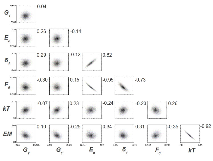
Figure 5 plots two-dimensional marginal distributions arising from the Bayesian/MCMC analysis for every pair of parameters in the spectral model (the priors used in the Bayesian/MCMC approach can be found in Table 4). It shows the effect each parameter has on the value of the other when finding highly probable parameter values to $\mathbf{\theta}$. Next to each plot the Spearman rank correlation coefficient for the indicated variables is shown. It can be seen that all the two-dimensional marginal distributions are elliptical, and the majority of them show that the probability of getting a particular parameter value is weakly correlated with the value of any other parameter. The exceptions to this for this flare are the emission measure ($EM$) and plasma temperature ($kT$) dependency, the dependency of the spectral normalization $F_{0}$ on the low-energy cutoff $E_{c}$ and the power law index $\delta_{1}$, and the $E_{c}$ versus $\delta_{1}$ correlation.

The first of these dependencies is anticipated through the definition of the thermal emission of the plasma (Equation 7), and the second two arise from the definition of the normalization. The normalization factor $F_{0}$ for this flare is defined as the total integrated electron flux  over all energies, and therefore clearly depends on the values of $E_{c}$ and $\delta_{1}$ (see Section 2). Figure 5 also shows a correlation between $E_{c}$ and $\delta_{1}$. This is obtained because the rate at which the X-ray spectrum flattens below $E_{c}$ depends on the value of $\delta_{1}$. The spectrum flattens more rapidly with decreasing photon energy for a steeper electron distribution (larger $\delta_{1}$) than for a flatter electron distribution. Therefore, for a given X-ray spectrum, a larger value of $\delta_{1}$ requires a higher value of $E_{c}$ to obtain the best fit to the spectrum. A similar correlation, for the same reason, is found between $E_{b}$ and $\delta_{2}$ in the fit to the July 23 flare spectrum (Figure 9).

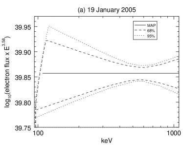
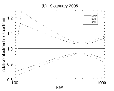
Figure 6(a) shows the (scaled) electron flux spectrum as a function of energy for the Bayesian/MCMC analysis. Figure 6(b) shows the ratio of the best fit electron spectrum to the 68% and 95% uncertainty estimates. Figures 4(a) and 6(c) show the probability density functions for total integrated electron number flux and electron power derived from the Bayesian/MCMC results. Uncertainty estimates for the electron flux spectrum as a function of energy are found in the following way. The electron flux spectrum for each Bayesian/MCMC-derived sample is calculated. The spectra are then ranked according to their posterior probability. The 68% curves are found by finding the highest and lowest values to the electron flux spectrum in each energy bin for the top 68% most probable samples (the 95% curves are found similarly), yielding the uncertainty estimates as shown in Figure 6(a). In each energy bin, the upper and lower uncertainties are approximately symmetric around the best ($\mathbf{\theta}^{MAP}$) value. Further, the probability density functions for the electron number flux and power (Figures 4(a) and 6(c)) are also approximately symmetrical around the mean and mode. This is not too surprising since the probability density functions (Figures 3, 4) for each parameter in the fit are also approximately symmetrical. Finally, the uncertainties in the values to the electron number and power are also well constrained.

Figure 3: Results from each of the four uncertainty analysis methods (Section 3) for the parameters of the thermal component of the total emission (a) $EM$ and (b) $kT$, from the model fit to the 19 January 2005 flare data. The dashed curve is the value of $\chi^{2}$ found by the $\chi^{2}$-mapping method (values are indicated by the right-hand plot axis). The normalized frequency distribution of values found by the Monte Carlo method is shown as a histogram (dot-dashed line). The marginal probability density function arising from the Bayesian/MCMC method is shown as a histogram (solid line). Values to these histograms are indicated by the left-hand plot axis. The horizontal lines show the uncertainty estimates calculated via the methods indicated (from top to bottom - covariance matrix, Bayesian/MCMC, Monte Carlo, and $\chi^{2}$-mapping), with the 68% and 95% uncertainty estimates indicated by larger and smaller vertical lines that cross those lines. The best-fit value $\hat{\mathbf{\theta}}$ found via nonlinear least-squares minimization (Section 3.1) is indicated by square plot symbols. The MAP value $\mathbf{\theta}^{MAP}$ is indicated by a $\times$-symbol. The mean, mode and median values calculated for each of the two distributions (arising from the Bayesian/MCMC and Monte Carlo analyses) are indicated by asterisks, diamonds and triangles respectively. These symbols are separated vertically scattered for clarity.

Figure 4: Results from each of the four uncertainty analysis methods (Section 3) for the parameters of the nonthermal component of the total flare emission (a) $F_{0}$, (b) $\delta_{1}$ and (c) $E_{c}$ (see Eq. 9) from the model fit to 19 January 2005 flare data. The type of data plotted, plot symbols and lines have the same meaning as in Figure 3.

Figure 5: Two dimensional marginal probability density functions for the parameters of the model used to fit the spectrum of the 19 January 2005 flare. These plots are found by integrating the posterior probability density function (found by the Bayesian/MCMC algorithm) over all the parameters excepting those indicated on the $x$- and $y$-axes. This is the extension into two dimensions of the definition of the one-dimensional marginal distribution function given by Equation 19 in Section 3.2.2. Each of these plots in this figure shows how the posterior probability density of the value of a given parameter depends on the value of another parameter, and so help visualize the shape of the full posterior probability density function. Indicated parameter ranges are the lowest and highest values found by the Bayesian/MCMC algorithm. Darker tones indicate a greater probability density. The number on the upper right of each plot is the Spearman rank correlation coefficient for the two parameters. For the 19 January 2005 flare, the distributions are all approximately elliptical. The majority of the distributions are weakly correlated; a minority ($EM$ versus $kT$, and $F_{0}$, $\delta_{1}$ versus $E_{c}$, $F_{0}$ versus $\delta_{1}$) show a high degree of correlation. The reasons for these strong correlations are discussed in Section 4.1.

Table 2: Parameter values and uncertainties derived for the four uncertainty estimation methods applied to the 19 January 2005 flare spectrum, as described in Section 2. The final column “Ratio” is defined as the ratio of the $\pm 95$% uncertainties to the $\pm 68$% uncertainties; for an exact Normal distribution the entry in this column would be $1.96,1.96$. Two ratios are quoted in order to reveal the presence of any relative asymmetry in the upper and lower uncertainty estimates, if present. See Section 3 for a detailed description of how the uncertainty estimates are found for each method.

Parameter	Method	Value	Uncertainties		Ratio
			68%	95%
$EM$ $(10^{49}\mbox{cm}^{-3})$	covariance matrix	2.31	$\pm$0.14	not calculated	not calculated
	$\chi^{2}$-mapping	“	-0.14, +0.15	-0.27, +0.31	1.94, 2.05
	Monte Carlo	“	-0.17, +0.12	-0.30, +0.27	1.75, 2.31
	Bayesian/MCMC	2.30	-0.14, +0.15	-0.27, +0.31	1.96, 2.04
$kT$ (keV)	covariance matrix	2.03	$\pm$0.02	not calculated	not calculated
	$\chi^{2}$-mapping	“	$\pm$0.02	$\pm$0.04	1.99, 2.01
	Monte Carlo	“	$\pm$0.02	-0.03, +0.04	2.13, 1.84
	Bayesian/MCMC	2.03	$\pm$0.02	$\pm$0.04	1.98, 2.03
$F_{0}$	covariance matrix	0.17	$\pm$0.01	not calculated	not calculated
(total integrated electron flux	$\chi^{2}$-mapping	“	$\pm$0.01	$\pm$0.02	1.90, 2.10
$10^{35}\mbox{ electrons}\mbox{ sec}^{-1}$)	Monte Carlo	“	$\pm$0.01	$\pm$0.01	1.87, 2.17
	Bayesian/MCMC	0.16	$\pm$0.01	$\pm$0.02	1.94, 1.96
$\delta_{1}$	covariance matrix	3.57	$\pm$0.03	not calculated	not calculated
	$\chi^{2}$-mapping	“	$\pm$0.04	-0.07, +0.08	1.95, 2.04
	Monte Carlo	“	-0.02, +0.04	-0.05, +0.07	2.15, 1.89
	Bayesian/MCMC	3.58	-0.03, + 0.04	-0.06, +0.07	1.88, 2.04
$E_{c}$ (keV)	covariance matrix	105	$\pm$3	not calculated	not calculated
	$\chi^{2}$-mapping	“	$\pm$4	$\pm$8	2.00, 2.00
	Monte Carlo	“	-3, 4	-6 , +7	2.10, 1.91
	Bayesian/MCMC	107	$\pm$4	-7, +8	1.85, 2.00

Figure 6: Electron spectrum results for the flare-injected electrons arising from the Bayesian/MCMC method for the 19 January 2005 flare. (a) Electron spectrum (flux (in units of erg $\mbox{keV}^{-1}$ $\mbox{s}^{-1}$) multiplied by $E^{3.58}$, where 3.58 is the MAP estimate $\delta_{1}$, the power law index of the flare-injected electron spectrum - see Table 2) with 68% and 95% credible interval spectra indicated by the dashed and dotted lines, respectively. The electron flux spectrum corresponding to $\theta^{MAP}$ is indicated by the solid line. (b) 68% and 95% credible intervals relative to the $\theta^{MAP}$ electron flux spectrum. In plots (a) and (b) curves with negative gradients indicate a behavior steeper than $E^{-\delta_{1}}$ and positive gradients indicate a behavior shallower than $E^{-\delta_{1}}$. Note also that the MAP spectrum extends to its low energy cutoff value; other lower probability spectra extend to values of $E_{c}$, which may be different to the MAP value of $E_{c}$. (c) Flare injected electron power probability density function, with 68% and 95% credible intervals indicated; the distribution mean/mode is indicated by the solid/dot-dashed vertical line. The total integrated electron flux injected by the flare is given in Figure 4(c).

4.2 23 July 2002

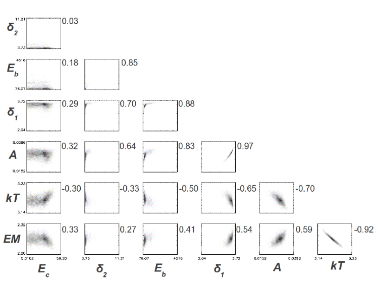
Figures 7, 8, 9 and Table 3 show the results for each of the four uncertainty estimation methods under consideration using the data and electron spectral model for the 23 July 2002 flare, as described in Section 2. It is clear from Figures 7, 8 and 9 that the $\chi^{2}$-hypersurface (or equivalently, the Bayesian posterior hypersurface - see Section 3.2.1) with respect to this model is quite different from that seen in the 19 January 2005 flare (Figures 3, 4 and 5). The mode values in the Bayesian/MCMC marginal distributions are noticeably shifted with respect to the Monte Carlo distributions. This is because the Bayesian/MCMC marginal distributions in Figures 7 and 8 are formed by integrating over a structured seven-dimensional space (Figure 9). The mode of the one-dimensional marginal distributions need not be at the $\theta^{MAP}$ or $\hat{\theta}$ value. Note however from Table 3 that the $\theta^{MAP}$ value is close to the $\hat{\theta}$ value, which is to be expected given the priors used in setting up the Bayesian posterior (see Appendix B) and the close correspondence between the $\chi^{2}$-hypersurface (Equation 10) and the Bayesian posterior (Equation 18).

Figures 7 (thermal model parameters) and 8 (non-thermal model parameters) show that the uncertainty estimates for specific parameters can depend on the uncertainty estimation method used. The methods used are influencing the uncertainty estimates for some parameters (Table 3). These uncertainty estimates behave quite differently from those expected from a Normal distribution, with the ratios of the 95% to 68% uncertainty estimates very different from 1.96. The reason for this is apparent when considering the two-dimensional Bayesian posterior marginal distributions as shown in Figure 9. Many of the distributions are structured, asymmetric, and show extended tails compared to those derived from the hypersurface of the 19 January 2005 analysis. The low-energy cutoff in particular shows significant deviation from a simple Normal distribution, as does the break energy $E_{b}$ and the slope of the spectrum above the break energy, parameterized by $\delta_{2}$. Many pairs of parameters have high magnitude correlation coefficients indicating strong interdependence of one value on another. Further, note that the correlation of $E_{c}$ with all other parameters is relatively weak. This indicates the relative independence of the low-energy cutoff from other features in the model, given the data.

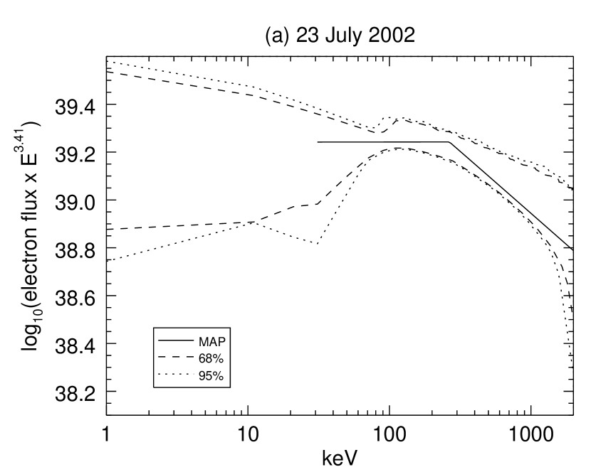
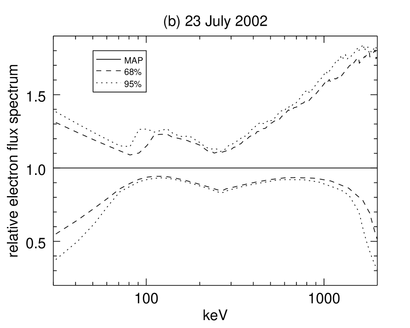
Figure 8(e) and 9 show that below around 25 keV, all values of $E_{c}$ are approximately equally likely, but also that $E_{c}<25$ keV does not constrain likely values of the emission measure $EM$, the thermal temperature $kT$, the normalization $A$ and the lower power-law index $\delta_{1}$. This leads to a wide range of possible electron-flux spectra at lower energies, the effect of which leads to wide 68% and 95% credible intervals of Figure 10(a). The uncertainty estimates for the electron flux in Figure 6(a) also show a widening at lower energies, but it is much less pronounced compared to that in Figure 10(a). The reason for this is that at lower values of $E_{c}$, the other parameter values in the model are constrained, and so there is a restricted range of electron flux spectra that is generated.

Figure 10 shows the (scaled) electron flux energy spectrum as a function of energy, along with probability density functions for total integrated electron number flux and electron power derived from the Bayesian/MCMC results. The wide 68% and 95% credible intervals of Figures 10(a, b) show that the electron spectrum becomes poorly constrained at low energies. Figures 10(c) and (d) are the electron number and power probability density functions, respectively (found by integrating the flare spectrum electron flux spectrum from $E_{c}$ to $E_{h}$). Both are asymmetric and show more pronounced tails when compared to the corresponding plots for the 19 January 2005 data (Figures 4(a) and 6(c)). This is due to the asymmetric low-energy cutoff probability density function which leads to a tail extending to high values in the probability density function of the electron number flux. Uncertainty estimates for the total number of flare-accelerated electrons and their energy are given in Figures 10(c, d). The probability density function for the energy can be integrated to determine lower limits to the energy contained in the flare-accelerated electrons whilst simultaneously supplying a probability estimate. The cumulative probability distribution function for the energy shows that there is a 95% probability that the energy in the flare-accelerated electrons is greater than $10^{28.0}$ erg sec^-1, and a 68% probability that it is greater than $10^{28.2}$.

Table 3: Parameter values and uncertainty estimates derived for the four uncertainty estimation methods applied to the 23 July 2002 flare spectrum, as described in Section 2. The final column “Ratio” is defined as the ratio of the $\pm 95$% uncertainties to the $\pm 68$% uncertainties; for an exact Normal distribution the entry in this column would be $1.96,1.96$. Two ratios are quoted in order to reveal the presence of any relative asymmetry in the upper and lower uncertainty estimates, if present. See Section 3 for a detailed description of how the uncertainty estimates are found for each method. The entry ‘not determined’ indicates that the value was not determinable by the method.

Parameter	Method	Value	Uncertainties		Ratio
			68%	95%
$EM$ $(10^{49}\mbox{cm}^{-3})$	covariance matrix	2.16	$\pm$0.08	not calculated	not calculated
	$\chi^{2}$-mapping		$\pm$0.04	$\pm$0.08	2.05, 1.99
	Monte Carlo		-0.05, 0.03	-0.09, 0.07	1.82, 2.28
	Bayesian/MCMC	2.17	$\pm$0.04	$\pm$0.08	1.89, 1.96
$kT$ (keV)	covariance matrix	3.18	$\pm$0.03	not calculated	not calculated
	$\chi^{2}$-mapping		$\pm$0.01	$\pm$0.02	1.97, 2.13
	Monte Carlo		$\pm$0.01	-0.02, 0.03	2.20, 1.87
	Bayesian/MCMC	3.18	$\pm$0.01	$\pm$0.03	1.93, 1.92
$A$	covariance matrix	0.028	$\pm$0.004	not calculated	not calculated
(electron flux at 50 keV,	$\chi^{2}$-mapping		-0.003, 0.002	-0.006, 0.005	2.15, 1.94
$10^{35}$ electrons $(\mbox{sec keV})^{-1}$)	Monte Carlo		-0.002, 0.003	-0.005, 0.005	2.21, 1.74
	Bayesian/MCMC	0.028	-0.003, 0.002	-0.006, 0.004	2.09, 1.76
$\delta_{1}$	covariance matrix	3.40	$\pm$0.16	not calculated	not calculated
	$\chi^{2}$-mapping		-0.14, 0.10	-0.36, 0.17	2.61, 1.78
	Monte Carlo		-0.14, 0.12	-0.34, 0.19	2.52, 1.61
	Bayesian/MCMC	3.41	-0.13, 0.08	-0.33, 0.13	2.55, 1.55
$E_{b}$ (keV)	covariance matrix	256	$\pm$135	not calculated	not calculated
	$\chi^{2}$-mapping		-77, 147	-123, 686	1.59, 6.67
	Monte Carlo		-77, 253	-121, 1319	1.58, 5.22
	Bayesian/MCMC	269	-147, 5615	-217, 1239	1.47, 2.01
$\delta_{2}$	covariance matrix	3.92	$\pm$0.11	not calculated	not calculated
	$\chi^{2}$-mapping		-0.08, 0.13	-0.13, 0.78	1.67, 5.67
	Monte Carlo		-0.07,0.23	-0.12, 3.27	1.74, 14.2
	Bayesian/MCMC	3.93	-0.11, 0.58	-0.18, 1.92	1.57, 3.33
$E_{c}$ (keV)	covariance matrix	32.0	$\pm$24.091	not calculated	not calculated
	$\chi^{2}$-mapping		-5.78, 5.05	not determined, 12.1	not determined, 2.4
	Monte Carlo		-6.86, 7.37	-20.7, 15.9	3.02, 2.16
	Bayesian/MCMC	31.2	-16.1, 11.7	-23.1, 19.1	1.44, 1.63

As was noted in Section 2.2, a different spectral normalization was used in the analysis of the 23 July 2002 flare compared to the 19 January 2005 flare. The package OSPEX implements the spectral normalization of the 19 January 2005 model spectrum using the integrated normalization factor, $F_{0}=AE_{c}^{1-\delta_{1}}/(\delta_{1}-1)$. This implementation of the flare spectral model therefore introduces a parameter dependence into the $\chi^{2}$-hypersurface between the normalization $A$, the low-energy cutoff and the spectral index $\delta_{1}$. However, since the low-energy cutoff for the 19 January 2005 flare is relatively well defined, the integrated flux $F_{0}$ is relatively well defined, and the MCMC algorithm can explore the $\chi^{2}$-hypersurface as a function of $F_{0}$ and $E_{c}$ with no difficulty. However, the low-energy cutoff is not well defined for the 23 July 2002 flare, and so the range of values to $F_{0}$ is large. Therefore when using the implementation of Equation 9 used in the analysis of the 19 January 2005 flare, the parameter space that must be covered by the MCMC algorithm is large due to the inherent dependence of $F_{0}$ on $E_{c}$. This was found to be prohibitive to an efficient MCMC search, and so an alternate implementation of Equation 9 was created for OSPEX (re-parameterization of the fitting function is a recommended tactic in creating better search spaces for MCMC (Gelman et al., 2003)). In this implementation, the normalization factor used to describe the spectrum is $A$, the value of the spectrum at the pivot value $E_{p}$. Moving to a different hypersurface for the same problem greatly improved the efficiency of the MCMC algorithm.

5 Discussion

5.1 Comparison of uncertainty analyses

The uncertainty analyses performed on both data-sets shows that the shape of the $\chi^{2}$-hypersurface has a significant effect on the values of the uncertainties found. All the uncertainty estimates found for the spectral parameters describing the 19 January 2005 flare data are similar, regardless of the method. The uncertainty estimates found for the spectral parameters describing the 23 July 2002 flare data depend on the method chosen.

Since the data have a large number of counts at almost all energies, the hypersurfaces described by Equation 10 and Equation 18 are almost identical. The two-dimensional marginal distributions for the 23 July 2002 flare data (Figure 9) shows structures which are not simple two-dimensional Normal distributions, and, since the two hypersurfaces described by Equation 18 and Equation 10 are almost identical, the $\chi^{2}$-hypersurface must have structures which are not simple two-dimensional Normal distributions. This means that one or more of the assumptions that lead to the assertion that the probability distribution for $\delta\mathbf{\theta}_{obs}$ is a multivariate Normal distribution around $\hat{\mathbf{\theta}}$ does not hold for this model applied to these flare data (Section 3.1.1). The non-Normal distribution shapes of Figure 9 suggest that the assumption that the spectral model is linear (or at least locally so within the range of the desired uncertainty calculation) is not satisfied (Press et al. 1992, p. 690). Hence, the covariance matrix and $\chi^{2}$-mapping methods cannot be expected to give reliable and consistent estimates in this case.

The shape of the $\chi^{2}$-hypersurface also influences the results of the Monte Carlo method. This can be seen in the results for the low-energy cutoff in the 23 July 2002 data-set (Figure 8e). It is expected that below a given energy $E_{plateau}$, all values of the low-energy cutoff are equally likely. This is because in this energy range the number of counts due to thermal emission greatly exceed the number due to the flare-injected electron flux spectrum, and so changing one value of $E_{c}$ over another makes no difference to the fit to the data - the value of $\chi^{2}$, or equivalently, the Bayesian posterior probability, are unaffected. Therefore, all values below $E_{plateau}$ are equally likely. The Monte Carlo method results do not show this; the results are clustered around the best-fit value and do not show the extension to lower energies as expected. Hence the uncertainty estimate arising from the Monte Carlo method does not conform to our prior expectation of what it should report.

In contrast, the Bayesian posterior hypersurface for the 19 January 2005 shows simple Normallike one-dimensional distributions (and so the assumptions behind the covariance matrix and $\chi^{2}$-mapping methods are approximately true) and give similar answers. The Monte Carlo method (Section 3.1.3) relies on finding local minima to simulated data which is statistically similar to the original data. This method works well in the 19 January 2005 analysis as the shape of the hypersurface (Figure 5) is dominated by a nearly Normal single minimum, a feature the method repeatedly finds in all the similar $\chi^{2}$-hypersurface. The $\chi^{2}$-mapping method does agree with the Bayesian/MCMC result in that the $\chi^{2}$-mapping method does indicate that below a certain value ($E_{plateau}$), all values of the low-energy cutoff are equally likely. However, the method cannot give a lower limit to the 95% uncertainty estimate since at no point does $\delta\chi^{2}=4$ for $E<E_{c}^{min}$ (Section 3.1.2).

The Bayesian/MCMC method samples the parameter space via the posterior probability and the Markov chain Monte Carlo algorithm (Section 3.2.1). The Bayesian interpretation of the posterior probability means that the parameter samples are found in proportion to how well they describe the data (values of $\mathbf{\theta}$ that have lower probability are less likely explanations of the data). The method does not make any assumptions about the nature of the hypersurface, as the other three methods do. Hence it agrees with the results from the methods of Section 3.1 when applied to simple hypersurfaces where the assumptions made by those methods are valid, but generates different results when those assumptions do not hold. Therefore, the Bayesian/MCMC method can, in principle, be used without having to invoke any special knowledge of the shape of the hypersurface and without making some simplifying assumptions.

5.2 Probability density functions of the parameters of the 23 July 2002 electron spectrum model

Figure 7: Results from each of the four uncertainty analysis methods (Section 3) for (a) $EM$ and (b) $kT$ from the model fit to the 23 July 2002 flare data. These plots follow the same convention as Figure 3. See Section 4 for more detail on these results.

Figure 8: Results from each of the four uncertainty analysis methods (Section 3) for (a) $A$, (b) $\delta_{1}$, (c) $E_{b}$, (d) $\delta_{2}$ and (e) $E_{c}$, from the model fit to the 23 July 2002 flare data. These plots follow the same convention as Figure 3. See Section 4 for more detail on these results.

Figure 9: Two dimensional marginal probability density functions for the parameters of the model used to fit the spectrum of the 23 July 2002 flare. In contrast to similar distributions plotted in Fig. 5 for the 19 January 2005 flare, some distributions are highly asymmetric within the parameter ranges found. The number on the upper right of each plot is the Spearman rank correlation coefficient for the abscissa versus the ordinate. There are many more moderately and strongly (anti-) correlated pairs of parameters for this flare model compared to the 19 January 2005 flare model. For some pairs of parameters (for example $\delta_{1}$ versus $A$ and $\delta_{2}$ versus $E_{b}$), the proportion of the space taken up by the high probability volume is relatively small, and for others (for example, $E_{c}$ versus $A$), it is relatively large. For the model applied to this flare spectrum, many of the resulting probability density functions do not show Normal distribution shapes. This indicates that the hypersurface for the model fit to these flare data has a more complicated structure than the hypersurface of the model fit to the 19 January 2005 flare.

Figure 10: Electron spectrum results for the flare-injected electrons arising from the Bayesian/MCMC method for the 23 July 2002 flare. (a) Electron spectrum (flux (in units of erg $\mbox{keV}^{-1}$ $\mbox{s}^{-1}$) multiplied by $E^{3.38}$) with 68% and 95% credible interval spectra indicated by the dashed and dotted lines, respectively. The electron flux spectrum corresponding to $\theta^{MAP}$ is indicated by the solid line. (b) 68% and 95% credible intervals (dashed and dotted lines, respectively) relative to the $\theta^{MAP}$ electron flux spectrum. (c) Flare injected electron number flux probability density function, with 68% and 95% credible intervals indicated. (d) Flare injected electron power probability density function, with 68% and 95% credible intervals indicated. In plots (c) and (d) the distribution mean/mode is indicated by the solid/dot-dashed vertical line.

Figures 7 and 8 show the marginal probability density functions of the parameter values arising from a Bayesian/MCMC treatment of the data analysis problem. It is notable that the distributions for $E_{b},\delta_{2}$ and $E_{c}$ are distinctly different from more symmetrical and Normal distribution-like distributions of the other parameters in the fit. The break energy $E_{b}$ and the power law index above the break $\delta_{2}$ are highly correlated (Figure 9) over a wide range of values. As $E_{b}$ increases, the value of $\delta_{2}$ increases. The mild curvature of the spectrum implied by these probability density functions is consistent with a wide range of near power-law electron flux spectrum models, leading to an ill-defined value for $E_{b}$ and softer power-law indices at higher values of $E_{b}$. A count spectrum that appears to come from emission that is mildly curved with respect to the radiation from the thick-target interaction of a flare-injected electron flux spectrum with a power law distribution could arise from an inaccurate X-ray albedo correction (Kontar et al., 2006) or from a non-uniform ionization within the target plasma (Su et al., 2009; Kontar et al., 2002).

The low-energy cutoff also has an interesting probability density function (also reproduced by the $\chi^{2}$-mapping analysis, Figure 8e). There is a peak in the Bayesian/MCMC low-energy cutoff probability density function at 31 keV, and a tail at lower energies where the thermal emission of the plasma dominates over the emission due to the flare-injected electron flux. We wish to estimate how much more likely the low-energy cutoff is close to the peak, compared to other parts of the probability density function. An estimate can be generated using the following procedure. If the probability density function of the low-energy cutoff were a Normal distribution $N(E_{cutoff},\sigma)$ (where $N(a,b)$ is a Normal distribution centered at $a$ with standard deviation $b$), then the total probability that $E_{c}$ lies in the range $E_{cutoff}-\sigma,E_{cutoff}+\sigma$ is about 68%. The maximum probability that $E_{c}$ lies in a $2\sigma$ wide range of values that does not overlap with the range $E_{cutoff}-\sigma,E_{cutoff}+\sigma$ is about 16%. Therefore the value of $E_{c}$ is about 4 times more likely to be in the range $E_{cutoff}-\sigma,E_{cutoff}+\sigma$ than in a $2\sigma$ wide range of values that does not overlap with the range $E_{cutoff}-\sigma,E_{cutoff}+\sigma$. Fitting the peak of the probability density function of Figure 8(e) with a Normal distribution yields a width $\sigma$ of about 5 keV. Applying the estimation procedure above on the probability density function of Figure 8(e) with $\sigma=5$ keV, it is found that $E_{c}$ is about 1.3 times more likely to be in the range 25-35 keV than in any other continuous window of values 10 keV wide. This is weak evidence for a peak in the range 25-35 keV.

Therefore, the probability density function is interpreted as providing evidence for the existence of an observable low-energy cutoff just above the region where the thermal emission dominates. If the low-energy cutoff was at higher energies, then the probability density function for $E_{c}$ would resemble more closely the probability density function seen in Figure 4(c) for the January 19 flare and therefore lower possible values to $E_{c}$ would lead to lower posterior probabilities (worse fits). If the low-energy cutoff was present at energies where the thermal emission dominates, then no peak in the probability density function for $E_{c}$ would be seen. Lower values would account for more of the flare-injected spectrum, and so lower values would be more probable. The probability $p(E_{c})$ would eventually plateau at some energy $E_{plateau}$ since the emission due to the flare-injected electron flux would be far less than the emission due to the thermal plasma below $E_{plateau}$, making all values of $E_{c}$ equally likely, as there is nothing to distinguish one value from another. However the observed $p(E_{c})$ is a combination of both; a peak in the probability density function with an approximately constant probability density at lower energies.

5.3 Flare electron number and energy probability density functions

The Bayesian/MCMC method allows for the construction of probability density functions for each flare (Figures 4(a) and 6(c), 10(c, d) of the number of flare-accelerated electrons and the energy they carry, fully expressing the correlated dependence of one variable on another (Figures 5, 9). Since the result is another probability density function, credible intervals for the number of electrons and their energy can also be calculated. In contrast, taking the set of 68% upper model parameter uncertainty estimates (or the other model parameter uncertainty estimates) from the the other methods cannot be used to calculate the corresponding 68% upper uncertainty estimate for the number of electrons and their energy. This is because there is no guarantee that that point on the $\chi^{2}$-hypersurface has a significant non-zero probability (or equivalently, lies in a hightly probable region of the model parameter hypersurface). In relatively simple hypersurfaces this may be true, but in highly correlated hypersurfaces such as in the analysis of the 23 July 2002 flare presented here, it may not be. As far as we are aware, this is the first time that flare electron number and energy probability density functions have been estimated from data.

A significant difference between the two flares studied is the uncertainty with which the model parameters are known. This leads to significant differences in how well the gross properties of the flare are known. The low-energy cutoff is not well constrained for the 23 July 2002 flare, leading to 68% and 95% credible intervals in the flare electron number and energy probability density functions that span orders of magnitude. Notably, the 23 July 2002 probability density functions are highly asymmetric and so lower values of flare electron number and energies are much less likely than higher values. It is interesting to note that there is a peak in the energy probability density function for the 23 July 2002 flare, even although there is a non-zero probability for $E_{c}$ down to the lower limit given by the prior for the low-energy cutoff. This is due to the peak in the marginal probability density function of $E_{c}$, which therefore defines a more probable total flare energy than those arising from the lower probability range $E_{c}<E_{plateau}$.

The estimate of the actual number of electrons and the energy they carry is also dependent on systematic errors related to the calibration of each of RHESSI detectors with each other. As was noted above, the systematic errors in the individual PHA bins are small compared to the systematic error in the overall sensitivity of each detector (Milligan & Dennis, 2009; Su et al., 2011). This means that the shape of the flare-accelerated electron spectrum suffers from a smaller error compared to the integral under the curve of the flare-accelerated spectrum. We therefore expect that the broad qualities of the shapes of the flare electron number and energy distributions will remain unchanged for each of the two flared studied; the 19 January 2005 results will remain approximately symmetric, and the 23 July 2002 results will remain quite asymmetric. We estimate that allowing for a 10% - 30% error in knowledge of the sensitivity of each detector would smooth out the distribution peak, and add another 0.1-0.2 in the logarithm (approximately) of the widths of the probability density functions. This estimated uncertainty is substantially more than the 95% estimated uncertainty in the case of the 19 January 2005 flare, but is substantially less than the 95% estimated uncertainty for the 23 July 2002 flare. This suggests that the uncertainty in the true value of the low-energy cutoff is a more important limiting factor in understanding the electron and energy content in RHESSI-observed flares than the detector calibration uncertainty.

5.4 Expanding the analysis

It is common in RHESSI data analysis to remove a background component from the observed count data to yield an estimate of the counts due solely to the flare. This background-subtracted data is then used in further analysis. Strictly, models for the background and the flare should be fit simultaneously since the observed counts are due to the background and the flare simultaneously. Therefore, the first improvement we will make is to fit both the flare response and background simultaneously. This will be done by including a simple parameterization of the pre- and post-flare hard X-ray flux observed by RHESSI into the flare model. The parameters of the background model will also require their own priors. The inclusion of a background model in the fit is expected to have an effect an higher energies, where the signal-to-noise ratio of the flare-accelerated electrons are smaller, such as in smaller flares.

The analyses presented here made use of data from one single detector. Our second improvement to the existing analysis will be to including data from more than one detector, which will increase the signal to noise ratio. In order to use data from more than one detector, information about the relative calibration of each detector will have to be included. This will be incorporated into priors for each detector that express the degree of uncertainty in their calibration. Since each detector is observing the same flare, the flare model will be the same across detectors. The posterior will be a product of the priors for the flare model plus background, a likelihood function for each detector, and a prior function expressing the degree of uncertainty in their calibration. The resulting posterior will express the increased knowledge that comes with a larger number of counts, but also the uncertainty in their relative calibration.

We note also that Bayesian data analysis provides a framework that can be used to compare the explanatory power of different models of the data whilst taking into account the number and type of variables in each model (Gregory, 2005). We will use Bayesian model comparison techniques to determine if RHESSI data can distinguish between different effects that may contribute to the observed spectra. In particular, we will re-analyze the 23 July 2002 data presented here using a model that incorporates the non-uniform ionization of the thick-target plasma (Su et al., 2009; Kontar et al., 2003). Such a model produces a curvature in flare-accelerated electron spectrum which may explain the high correlation between the break energy $E_{b}$ and the value of $\delta_{2}$ (Section 4.2).

6 Conclusions

This paper describes in some detail four methods that can be used to estimate the uncertainties in parameters of flare models fit to RHESSI hard X-ray flare data. Three of the four methods – covariance matrix, Monte Carlo, and $\chi^{2}$-mapping – measure scale-sizes in the $\chi^{2}$-hypersurface (or related hypersurfaces) and call them uncertainty estimates. We have shown that care must be taken in relying upon these uncertainty measurements, as we have seen that they need not agree with our expectation of what an uncertainty estimate should report, or with each other. The fourth method, Bayesian data analysis, can answer the question “what is the uncertainty in this parameter?” by calculating a probability density function for that parameter through the marginalization procedure of Section 3.2.2 without making any further assumptions about the number of counts in each bin (see Section 3.2.1). The fourth method broadly agrees with the other three in the case of the 19 January 2005 flare. Each method generates different uncertainty estimates for the 23 July 2002 flare.

The source of the different uncertainty estimates is the shape of the $\chi^{2}$-hypersurface parameterized by the flare model. hypersurfaces that broadly conform to the assumptions underlying the covariance matrix, Monte Carlo, and $\chi^{2}$-mapping methods yield consistent uncertainty estimates that agree with each other and those from the Bayesian/MCMC approach. Conversely, hypersurfaces that break those assumptions yield method-dependent results. The Bayesian/MCMC approach makes no assumptions on the nature of the hypersurface. Further, the position of the low-energy cutoff in relation to the region where thermal X-ray emission dominates is crucial in determining the shape of the hypersurface. Most flares are thought to have a low-energy cutoff close to or at the region of thermal emission dominance. The Bayesian/MCMC method presented here handles both flare analyses without regard to the location of the low-energy cutoff, and makes no assumption about the $\chi^{2}$-hypersurface or Bayesian posterior probability hypersurface. The Bayesian/MCMC method was the only method to generate an uncertainty estimate of the low-energy cutoff that reflects our intuition of how it is constrained by the data, for both flares studied. Since the $\chi^{2}$-mapping approach does partially map the space around $\hat{\mathbf{\theta}}$, it is perhaps the best of the three non-Bayesian based methods that can give an indication that the $\chi^{2}$-hypersurface contains features that are not similar to Normal distribution shapes. If the $\chi^{2}$-hypersurface does contain features not anticipated by the covariance matrix, Monte Carlo, and $\chi^{2}$-mapping methods, then we suggest a Bayesian/MCMC approach is warranted if reliable uncertainty estimates are desired.

The 23 July 2002 flare shows evidence for the existence of a low-energy cutoff in the range 25–35 keV, just above the region where the thermal emission dominates. The probability density function of the low-energy cutoff shows significant non-zero probability below 25 keV, and zero probability above 50 keV. This peak is important, as it leads to highly asymmetric probability density functions for the total number of flare electrons accelerated by the flare, and the energy they carry, in which the upper limit to these quantities are poorly constrained. In each of these quantities, the 95% upper credible limit is orders of magnitude larger than the MAP value, whilst the 95% lower limit is within one order of magnitude of the MAP value. In comparison, the MAP values for the same quantities of the 19 January 2005 flare lie are approximately centered within a tenth of a decade. This points to the importance of the low-energy cutoff probability density function in determining the quality of our knowledge of the gross properties of the flare.

Further work will involve improving the modeling of RHESSI observations by including data from other RHESSI detectors, incorporating the simultaneous fitting of the background emission at the same time as the flare model, and testing different models of flare emission for the same flare.

Appendix A Parallel tempering Markov chain Monte Carlo algorithm

A significant problem in MCMC is ensuring that the posterior is explored sufficiently. The first MCMC algorithms used in this study did not generate the expected marginal probability distribution of the low-energy cutoff $E_{c}$ for the flare of 23 July 2002. The distribution arising from these MCMC algorithms showed a single peak with $p(E_{c})=0$ below some value. The expected distribution contains a plateau region of approximately constant non-zero probability density for values $E_{c}<E_{plateau}$ for some value of $E_{plateau}$ determined from the data (see also Section 5.1). The difference between the expected distribution and those derived from the MCMC algorithm may be due to either insufficient exploration of the posterior by the MCMC algorithm, or to some previously unexpected feature in the flare spectrum. To test these explanations, a new MCMC algorithm was implemented to more fully explore the parameter space of the posterior distribution.

The parallel tempering algorithm allows one to explore the parameter space by optionally making easier moves in related spaces (Gregory, 2005). Parallel tempering is based on simulated tempering. This scheme mimics the physical process of annealing, whereby a metal is heated and cooled in order to obtain a more crystalline and therefore lower energy structure. By analogy, simulated tempering uses a set of discrete values of a temperature parameter $T$ to label and describe flatter versions of the original posterior distributions. The value $T=1$ is reserved for the the original posterior distribution. Higher values of $T$ correspond to flatter distributions. In simulated tempering, the distribution is ‘warmed up’ by increasing $T$. In these flatter versions, it is easier for the sampler to jump out of local minima and explore the full posterior to find the global minimum. Inferences are drawn from the $T=1$ sampler.

As above, let $p(H|\mbox{$\mathbf{D}$},\mathcal{I})$ be the target posterior distribution we want to sample; by Bayes’ theorem

$$p(H|\mbox{$\mathbf{D}$},\mathcal{I})\propto p(H|\mathcal{I})\times p(\mbox{$\mathbf{D}$}|H,\mathcal{I})$$ (A1)

where we have dropped the normalization factor $1/p(\mbox{$\mathbf{D}$}|\mathcal{I})$. Other posterior distributions at different annealing temperatures $\beta\equiv 1/T$ are constructed as

$$\pi(H|\mbox{$\mathbf{D}$},\mathcal{I},\beta) = p(H|\mathcal{I})p(\mbox{$\mathbf{D}$}|H,\mathcal{I})^{\beta}$$ (A2)

$$= p(H|\mathcal{I})\exp\left(\beta\log\left[p(\mbox{$\mathbf{D}$}|H,\mathcal{I})\right]\right)$$ (A3)

where $0<\beta\leq 1$. The parameter $\beta$ varies from 0 to 1; $\beta=1$ corresponds to the original, target distribution, with lower values corresponding to flatter (higher temperature) versions of the target distribution.

In parallel tempering, multiple MCMC chains are run in parallel at $n_{T}$ temperatures $\{1,\beta_{0},\beta_{1},...,\beta_{n_{T}}\}$ for $n_{T}>1$. At intervals, proposals are made to swap the parameter states at adjacent but randomly selected temperatures. For example, at iteration $t$, suppose that the sampler at $\beta_{i}$ has a parameter $H_{t,i}$, and $\beta_{i+1}$ has a parameter state $H_{t,i+1}$. These are the candidate parameter states for swapping. The swap is accepted with probability

$$r=\min\left\{\frac{\pi\left(H_{t,i+1}|\mbox{$\mathbf{D}$},\beta_{i},\mathcal{I}\right)\pi\left(H_{t,i}|\mbox{$\mathbf{D}$},\beta_{i+1},\mathcal{I}\right)}{\pi\left(H_{t,i}|\mbox{$\mathbf{D}$},\beta_{i},\mathcal{I}\right)\pi\left(H_{t,i+1}|\mbox{$\mathbf{D}$},\beta_{i+1},\mathcal{I}\right)}\right\}.$$ (A4)

The swap is accepted if $U_{1}\approx\mbox{Uniform}[0,1]\leq r$, that is, if a number $U_{1}$ drawn from a uniform random distribution between zero and 1, is less than or equal to $r$. If the swap is accepted, then the parameter states are swapped: the chain indexed $i$ now has parameter state $H_{t,i+1}$, and the chain indexed $i+1$ now has parameter state $H_{t,i}$. This swapping process propagates information across the parallel simulations. At higher temperatures, the algorithm can explore very different locations in the posterior parameter space. At lower temperatures, the algorithm can improve local knowledge of the space around minima. Swapping allows highly probable parameter states to propagate down to lower temperatures where they can be explored locally. The swap itself need not be proposed at every iteration. Gregory (2005) implements an example parallel tempering algorithm by allowing a swap on average once every $n_{s}$ iterations: the swap is only performed if the value of $U_{2}$, drawn from a uniform distribution between zero and 1, is less than or equal to $1/n_{s}$.

Each of the MCMC chains uses the Metropolis-Hastings algorithm (Gregory, 2005) to explore each $\pi(H|\mbox{$\mathbf{D}$},\mathcal{I},\beta)$. Normal distributions were used as the proposal distributions for Metropolis-Hastings algorithm. Widths for each proposal distribution were found after making several shorter exploratory runs of the $\beta=1$ chain with an adaptive algorithm that varied the proposal distribution with to generate an acceptance ratio in the range $0.16\rightarrow 0.30$ (Gelman et al., 2003). For each variable $\theta$ in each spectral model, a uniform prior is assumed, that is, $p(\theta)=1/(\theta_{1}-\theta_{0})$ for $\theta_{0}\leq\theta\leq\theta_{1}$ and $p(\theta)=0$ otherwise. The lower ($\theta_{0}$) and upper ($\theta_{1}$) values are constants. The limits($\theta_{0}$) and upper ($\theta_{1}$) and the proposal distribution step-size are given in Tables 4.

As is described in the main text, the parallel tempering MCMC algorithm produces marginal distributions of $E_{c}$ for the 23 July 2002 flare consistent with expectations. The parallel tempering MCMC algorithm described here was used in the analysis of both the 19 January 2005 and 23 July 2002 flares.

Appendix B Implementation of the parallel tempering Markov chain Monte Carlo algorithm

The results described in the paper arise from implementing the parallel tempering algorithm described in Section A. Five temperatures in the algorithm are used: $\beta={1,0.75,0.5,0.25,0.01}$. Each simulation takes 50,000 samples (five times as many samples as the Monte Carlo approach of Section 3.1.3). The simulation is run ten times with a different starting point chosen uniformly randomly in the volume $\mathbf{\theta}_{0}-5\mathbf{s},\mathbf{\theta}_{0}+5\mathbf{s}$, where $\mathbf{s}$ is the size of the proposal distribution step size. The proposal distribution step size is the square root of the diagonal elements of the covariance matrix of a least squares fit calculated at $\mathbf{\theta}_{0}$. The last half of the samples are considered post burn-in, and are retained. Convergence between and within the 10 simulation runs is assessed using the $R$ measurement from Gelman et al. (2003). In all cases, the $R$-measurement was below approximately 1.1, which may be taken as indicating convergence (Gelman et al., 2003; van Dyk et al., 2001).

Table 4: Details of the prior variable ranges and the proposal distribution step-size used in the Bayesian/MCMC analysis of the 19 January 2005 and 23 July 2002 flare data. Priors for each variable are uniform within the stated ranges. Each proposal distribution is Normal, with width as indicated. See Section 2 for more detail on the choice of model, and Appendix A for more detail on the implementation of the Bayesian/MCMC analysis. the proposal distributions are all Normal.

Flare	Parameter	Prior range	Proposal distribution width
19 January 2005	$EM$	$0.77\rightarrow 6.94$	0.01
	$kT$	$0.68\rightarrow 6.08$	0.01
	$F_{0}$	$0.01\rightarrow 1000$	0.0004
	$\delta_{1}$	$1.1\rightarrow 20$	0.002
	$E_{c}$	$6.8\rightarrow 290$	0.17
	$G_{1}$	$3334\rightarrow 33347$	821
	$G_{2}$	$1279\rightarrow 12790$	283
23 July 2002	$EM$	$0.9\rightarrow 8.14$	0.004
	$kT$	$0.5\rightarrow 8.0$	0.001
	$A$	$0.002\rightarrow 0.3$	0.0003
	$\delta_{1}$	$1.1\rightarrow 50$	0.014
	$E_{b}$	$50\rightarrow 32000$	7.5
	$\delta_{2}$	$1.1\rightarrow 50$	0.007
	$E_{c}$	$0.01\rightarrow 50$	0.57

Appendix C Normality of the marginal distributions

The normality of the univariate marginal distributions was assessed using Q-Q (quantile-quantile) plots (Figures 11 and 12). A Q-Q plot is a graphical method of comparing two different distributions, and is constructed as follows. The cumulative distribution function of a random variable $X$ is defined as

$$F_{X}(x)=P(X\leq x)$$ (C1)

that is, the probability that the random variable $X$ takes on a value less than or equal to $x$. The function $F_{X}(x)$ is monotonically increasing in the range zero to one. The inverse of $F_{X}$ is called the quantile function, $Q$, and is defined as

$$Q_{X}(r)=x\mbox{ if }F_{X}(x)=r.$$ (C2)

If $F_{X}$ is a one-to-one function, the inverse $Q$ is uniquely determined. If the function $F_{X}$ is not one-to-one the inverse $Q$ can be defined as the weighted average of all relevant points. The definition of the quantile function applies to random variables or sample distributions. The Q-Q plots shown in Figures 11 and 12 show a set of open circles and a straight line. A circle is plotted at the point where the abscissa and the ordinate are the values of quantile functions for the standard Normal distribution $N(0,1)$ and the marginal distribution, for a given value of probability $r$. A straight line is drawn through the points defined by the quantile functions for the standard Normal distribution and a Normal distribution $N\left(\hat{\theta_{i}},\hat{\sigma_{\theta_{i}}^{2}}\right)$, where

$$\hat{\theta_{i}}=\frac{1}{N_{S}}\sum_{j=1}^{N_{S}}[\theta_{i}]_{j}$$

and

$$\hat{\sigma_{\theta_{i}}^{2}}=\frac{1}{N_{S}-1}\sum_{j=1}^{N_{S}}\left\{[\theta_{i}]_{j}-\hat{\theta_{i}}\right\}^{2}$$

are estimated from the $N_{S}$ samples of the parameter $\theta_{i}$, $1\leq i\leq N_{\mathbf{\theta}}$. The straight line enables an assessment of how closely the marginal distribution follows a Normal distribution, and where any deviations occur. The quantile function for the standard Normal distribution function is called the probit function and is defined as

$$\mbox{probit}(r)=\sqrt{2}\mbox{ erf}^{-1}(2r-1),r\in(0,1)$$ (C3)

where $\mbox{erf}^{-1}(x)$ is the inverse error function. The probit function gives the value of a $N(0,1)$ random variable associated with specified cumulative probability $r$, for example:

$$\mbox{probit}(0.025)\simeq-1.96\simeq-\mbox{probit}(0.975).$$ (C4)

Therefore, and conveniently, the abscissa in the Q-Q plots can be understood as multiples of the standard deviation away from the mean. The Q-Q plots were implemented using the ‘R’ statistical computing environment, available from the R Project for Statistical Computing (R Development Core Team, 2011).

Figure 11: Q-Q plots for the Bayesian/MCMC samples of the 19 January 2005 model spectrum parameter values. All parameters are approximately Normally distributed in the range $-2,+2$ quantiles about the estimated mean. The tails of the distributions show deviations away from a true Normal distribution. Curvature of the sample distribution at negative quantiles indicates that the tail is thinner than that expected from the sample Normal distribution $N\left(\hat{\theta_{i}},\hat{\sigma_{\theta_{i}}^{2}}\right)$. Similarly, curvature of the sample distribution at large positive quantitles indicates that the tail is fatter than that expected from the sample Normal distribution $N\left(\hat{\theta_{i}},\hat{\sigma_{\theta_{i}}^{2}}\right)$.

Figure 12: Q-Q plots for the Bayesian/MCMC samples of the 23 July 2002 model spectrum parameter values. The two thermal parameters of the model $EM$ and $kT$ appear to be approximately Normally distributed; the remaining non-thermal parameters ($A$, $\delta_{1}$, $E_{b}$, $\delta_{2}$ and $E_{c}$) are clearly not Normally distributed.

References

- Brown (1971) Brown, J. C. 1971, Sol. Phys., 18, 489
- Brown et al. (2006) Brown, J. C., Emslie, A. G., Holman, G. D., et al. 2006, ApJ, 643, 523
- Brown et al. (2003) Brown, J. C., Emslie, A. G., & Kontar, E. P. 2003, ApJ, 595, L115
- Cash (1979) Cash, W. 1979, ApJ, 228, 939
- Dere et al. (1997) Dere, K. P., Landi, E., Mason, H. E., Monsignori Fossi, B. C., & Young, P. R. 1997, A&AS, 125, 149
- Dere et al. (2009) Dere, K. P., Landi, E., Young, P. R., et al. 2009, A&A, 498, 915
- Emslie et al. (2005) Emslie, A. G., Dennis, B. R., Holman, G. D., & Hudson, H. S. 2005, Journal of Geophysical Research (Space Physics), 110, 11103
- Emslie et al. (2004) Emslie, A. G., Kucharek, H., Dennis, B. R., et al. 2004, Journal of Geophysical Research (Space Physics), 109, 10104
- Feldman et al. (1992) Feldman, U., Mandelbaum, P., Seely, J. F., Doschek, G. A., & Gursky, H. 1992, ApJS, 81, 387
- Gelman et al. (2003) Gelman, A., Carlin, J. B., Stern, H. S., & Rubin, D. B. 2003, Bayesian Data Analysis, Second Edition (Chapman & Hall/CRC Texts in Statistical Science), 2nd edn. (Chapman and Hall/CRC)
- Gregory (2005) Gregory, P. C. 2005, Bayesian Logical Data Analysis for the Physical Sciences: A Comparative Approach with ‘Mathematica’ Support (Cambridge University Press)
- Holman et al. (2003) Holman, G. D., Sui, L., Schwartz, R. A., & Emslie, A. G. 2003, ApJ, 595, L97
- Holman et al. (2011) Holman, G. D., Aschwanden, M. J., Aurass, H., et al. 2011, Space Sci. Rev., 159, 107
- Humphrey et al. (2009) Humphrey, P. J., Liu, W., & Buote, D. A. 2009, ApJ, 693, 822
- Jaynes (2003) Jaynes, E. T. 2003, Probability Theory (Cambridge University Press, Cambridge, UK)
- Kashyap & Drake (1998) Kashyap, V., & Drake, J. J. 1998, ApJ, 503, 450
- Kontar et al. (2002) Kontar, E., Brown, J., & McArthur, G. 2002, Solar Physics, 210, 419, 10.1023/A:1022494318540
- Kontar et al. (2003) Kontar, E. P., Brown, J. C., Emslie, A. G., et al. 2003, ApJ, 595, L123
- Kontar et al. (2008) Kontar, E. P., Dickson, E., & Kašparová, J. 2008, Sol. Phys., 252, 139
- Kontar et al. (2006) Kontar, E. P., MacKinnon, A. L., Schwartz, R. A., & Brown, J. C. 2006, A&A, 446, 1157
- Kontar et al. (2011) Kontar, E. P., Brown, J. C., Emslie, A. G., et al. 2011, Space Sci. Rev., 159, 301
- Lee et al. (2011) Lee, H., Kashyap, V. L., van Dyk, D. A., et al. 2011, ApJ, 731, 126
- Lin & Hudson (1971) Lin, R. P., & Hudson, H. S. 1971, Sol. Phys., 17, 412
- Lin & Hudson (1976) —. 1976, Sol. Phys., 50, 153
- Lin et al. (2002) Lin, R. P., Dennis, B. R., Hurford, G. J., et al. 2002, Sol. Phys., 210, 3
- Lin et al. (2003) Lin, R. P., Krucker, S., Hurford, G. J., et al. 2003, ApJ, 595, L69
- Mazzotta et al. (1998) Mazzotta, P., Mazzitelli, G., Colafrancesco, S., & Vittorio, N. 1998, A&AS, 133, 403
- Milligan & Dennis (2009) Milligan, R. O., & Dennis, B. R. 2009, ApJ, 699, 968
- Murphy et al. (1991) Murphy, R. J., Ramaty, R., Reames, D. V., & Kozlovsky, B. 1991, ApJ, 371, 793
- Piana et al. (2003) Piana, M., Massone, A. M., Kontar, E. P., et al. 2003, ApJ, 595, L127
- Press et al. (1992) Press, W. H., Teukolsky, S. A., Vetterling, W. T., & Flannery, B. P. 1992, Numerical recipes in FORTRAN. The art of scientific computing (Cambridge: University Press, —c1992, 2nd ed.)
- R Development Core Team (2011) R Development Core Team. 2011, R: A Language and Environment for Statistical Computing, R Foundation for Statistical Computing, Vienna, Austria, ISBN 3-900051-07-0
- Smith et al. (2002) Smith, D. M., Lin, R. P., Turin, P., et al. 2002, Sol. Phys., 210, 33
- Su et al. (2011) Su, Y., Holman, G. D., & Dennis, B. R. 2011, ApJ, 731, 106
- Su et al. (2009) Su, Y., Holman, G. D., Dennis, B. R., Tolbert, A. K., & Schwartz, R. A. 2009, ApJ, 705, 1584
- Tandberg-Hanssen & Emslie (1988) Tandberg-Hanssen, E., & Emslie, A. G. 1988, The physics of solar flares (Cambridge and New York, Cambridge University Press)
- Thompson (2006) Thompson, W. T. 2006, A&A, 449, 791
- van Dyk et al. (2001) van Dyk, D. A., Connors, A., Kashyap, V. L., & Siemiginowska, A. 2001, ApJ, 548, 224
- Warmuth et al. (2009) Warmuth, A., Holman, G. D., Dennis, B. R., et al. 2009, ApJ, 699, 917
- Wasserman (2003) Wasserman, L. 2003, All of Statistics: A Concise Course in Statistical Inference (Springer Texts in Statistics) (Springer)