Breather and Rogue Wave solutions of a Generalized Nonlinear Schrödinger Equation

Abstract

In this paper, using the Darboux transformation, we demonstrate the generation of first-order breather and higher-order rogue waves from a generalized nonlinear Schrödinger equation with several higher-order nonlinear effects representing femtosecond pulse propagation through nonlinear silica fiber. The same nonlinear evolution equation can also describes the soliton-type nonlinear excitations in classical Heisenberg spin chain. Such solutions have a parameter $\gamma_{1}$, denoting the strength of the higher-order effects. From the numerical plots of the rational solutions, the compression effects of the breather and rogue waves produced by $\gamma_{1}$ are discussed in detail.

I Introduction

It is well known that one of the most challenging aspects of modern science and technology is the nonlinear nature of the system, which is considered to be fundamental to the understanding of many natural phenomena. In recent years, nonlinear science has emerged as a powerful subject for explaining the mysteries of the challenging nature. Nonlinearity is a fascinating occurrence of nature whose importance has been well appreciated for many years, in the context of large amplitude waves or high-intensity laser pulses observed in various fields ranging from fluids to solid state, chemical, biological, nonlinear optical, and geological systems GPA1 ; AH1 ; LFM ; KP1 ; KP2 ; JRT1 ; FA1 ; FA2 ; YSK . This fascinating subject has branched out in almost all areas of science, and its applications are percolating through the whole of science. In general, nonlinear phenomena are often modeled by nonlinear evolution equations exhibiting a wide range of high complexities in terms of different linear and nonlinear effects. In recent years, the advent of high-speed computers, many advanced mathematical software, and development of many sophisticated and systematic analytical methods in the study of the nonlinear phenomena and also supported by many experiments have encouraged both theoretical and experimental research. In the past few decades, nonlinear science has experienced an explosive growth by the invention of several exciting and fascinating new concepts, such as solitons, dispersion-managed solitons, dromions, rogue waves, similaritons, supercontinuum generation, complete integrability, fractals, chaos, etc. GPA1 ; AH1 ; LFM ; KP1 ; KP2 ; JRT1 ; FA1 ; FA2 ; YSK ; GPA2 ; NN1 . Many of the completely integrable nonlinear partial differential equations (NPDEs) admit one of the most striking aspects of nonlinear phenomena called soliton, which describe soliton as a universal character, and they are of great mathematical as well as physical interest, too. The study of the solitons and other related issues of the construction of the solutions to a wide class of NPDEs have become one of the most exciting and extremely active areas of research in science and technology for many years.

In addition to several developments in soliton theory, recent developments in modulational instability (MI) have also been widely used to explain why experiments involving white coherent light supercontinuum generation (SCG), admit a triangular spectrum. Such universal triangular spectra can be well described by the analytical expressions for the spectra of Akhmediev breather solutions at the point of extreme compression. In the context of the NLS equation, Peregrine already in Ref. peregrine had identified the role of MI in the formation of patterns resembling freak waves or rogue wave (RW); these theoretical results were later supported by several experiments. Rogue waves in the ocean are localized large amplitude waves on a rough background, which have two remarkable characteristics: (1) “appear from nowhere and disappear without a trace” akhmediev1 , (2) exhibit one dominant peak. RWs have recently appeared in several areas of science. Particularly in photonic crystal fibers, RWs have been well established in connection with SCG soli1 . This actually has stimulated research for RWs in other physical systems and has paved the way for many important applications, including the control of RWs by means of SCG soli2 ; dudley , as well as studies in superfluid Helium ganshin , Bose-Einstein condensates konotop1 , plasmas ruderman ; shukla , microwave hohmann , capillary phenomena shats , in telecommunication data streams vergeles , inhomogeneous media arecchi , water experiments akhmediev3 ; akhmediev4 , and so on. More recently, Kibler et al. akhmediev2 , using their elegant experimental apparatus in optical fibers, were able to generate femtosecond pulses with strong temporal and spatial localization and near-ideal temporal Peregrine soliton characteristics.

In the recent past, several equations have been shown to admit the rogue wave solutions. For example, in addition to the NLS equation, the Hirota equation akhmediev5 ; he1 ; lu1 , the first-type derivative NLS equation he2 , the third-type DNLS equation he3 , the Fokas-Leneels equation xuhepfoakseq , the NLS-MB equations he4 , the Hirota Maxwell-Bloch(MB) equations lihephmb , the Sasa-Satsuma equation Bandelow , the discrete Ablowitz-Ladik and Hirota equation akhmediev6 , the two-component NLS equations akhmediev6b ; guo1 ; fabio1 , the three-components NLS equations qin1 , the variable coefficient NLS akhmediev7 ; taki1 ; yan1 ; he5 ; liu1 , the variable coefficient derivative NLS he6 , and the variable coefficient higher-order NLS (VCHNLS) zhang1 , the rogue waves in dissipative systems Philippe are a few of the nonlinear evolution equations that admit RWs. From the above studies, it is clear that one of the possible generating mechanisms hezhangwangpf2012 for the higher-order RW is the interaction of the multiple breathers possessing the same and the very particular frequency of the underlying equation.

In recent years, there has been a considerable interest in the study of the nonlinear excitations of the spin chains with competing bilinear and biquadratic interactions. In particular, the complete integrability and nonlinear excitations of spin chains with spin magnitude $S>1$ has been established if suitable polynomials in ($S_{i},S_{j}$) are added to the original bilinear Heisenberg spin Hamiltonian. In this connection and also from the mathematical point of view, it is of interest to study the influence of the biquadratic interactions on the integrability of the Heisenberg bilinear spin chain in the classical limit as well. Considering the above points, one of the authors of this paper, has investigated the integrability aspects of a classical one-dimensional isotropic biquadratic Heisenberg spin chain in its continuum limit up to order $O(a^{4})$ in the lattice parameter through a classical differential geometric approach kpspin1 ; kpspin2 ; kpspin3 and investigated the soliton and integrability aspects of the corresponding generalized nonlinear Schrödinger Equation (GNLSE). This equation is given by kpspin1

$$iq_{{t}}+q_{{xx}}+2{q}|q|^{2}+\gamma_{1}\left(q_{{xxxx}}+6{q_{x}^{2}}q^{*}+4q|q_{x}|^{2}+8|q|^{2}q_{xx}+2{q}^{2}q^{*}_{{xx}}+6|q|^{4}{q}\right)=0.$$ (1)

Here, $q(x,t)$ is the complex envelope and $\gamma_{1}$ denotes the strength of higher-order linear and nonlinear effects. When we consider the propagation of ultra short pulse propagation through optical fiber, i.e, less than 100-fs pulses, it has been shown that higher-order dispersion, self-steepening, self-frequency, and quintic effects should be included in the model. The above equation has been shown to be integrable and admits exact soliton solutions and also gauge equivalent to Heisenberg spin chain equation. Thus, it is an interesting problem to find how these higher-order terms will affect the breather and rogue wave in an associated optical system and spin system by means of changing the value of $\gamma_{1}$. It is our prime aim to answer this problem in this paper.

The paper is organized as follows. In Sec. II, the Lax pair and the Darboux transformation (DT) are introduced. In Sec. III, we shall give the first-order breather and it’s limit of infinitely large period. In Sec. IV, higher-order rogue waves are given. The compression effects on the breather and rogue waves produced by the higher-order terms of GNLSE are given in Secs. III and IV, respectively. Section V is devoted to conclusions.

II Lax Pair and Darboux transformation

As discussed above, in this section, we would like to recall the Lax pair of GNLSE kpspin1 ; kpspin2 ; kpspin3 and to show its Darboux transformation. According to the AKNS formalism, Lax pair for Eq. (1) is written as

$$\Phi_{x}=M\Phi,\Phi_{t}=N\Phi$$ (2)

with the following matrices:

$$M=i\lambda U_{0}+U_{1}=i\lambda\left(\begin{array}[]{cc}-1&0\\ 0&1\end{array}\right)+\left(\begin{array}[]{cc}0&q\\ -q^{*}&0\end{array}\right)=\left(\begin{array}[]{cc}-i\lambda&q\\ -q^{*}&i\lambda\end{array}\right),$$

and $N=8i\gamma_{1}V_{4}-2iV_{2}$. Here,

$$V_{2}=\left(\begin{array}[]{cc}{\lambda}^{2}-\frac{1}{2}\,qq^{*}&iq\lambda-\frac{1}{2}q_{{x}}\\ -iq^{*}\,\lambda-\frac{1}{2}\,q^{*}_{{x}}&-{\lambda}^{2}+\frac{1}{2}\,qq^{*}\end{array}\right),V_{4}=\left(\begin{array}[]{cc}A_{4}&B_{4}\\ C_{4}&-A_{4}\end{array}\right),$$

$$\begin{split}A_{4}=&{\lambda}^{4}-\frac{1}{2}qq^{*}{\lambda}^{2}+\frac{i}{4}\left(qq^{*}_{{x}}-q_{{x}}q^{*}\right)\lambda+\frac{1}{8}(3{q}^{2}{q^{*}}^{2}+q^{*}\,q_{{x,x}}+qq^{*}_{{x,x}}-q_{{x}}q^{*}_{{x}}),\\ B_{4}=&iq{\lambda}^{3}-\frac{1}{2}q_{{x}}{\lambda}^{2}-\frac{i}{4}\left(q_{{x,x}}+2{q}^{2}q^{*}\right)\lambda+\frac{1}{8}(q_{{x,x,x}}+6\,qq^{*}\,q_{{x}}),\\ C_{4}=&-iq^{*}\,{\lambda}^{3}-\frac{1}{2}q^{*}_{{x}}{\lambda}^{2}+\frac{i}{4}\left(q^{*}_{{x,x}}+2q{q^{*}}^{2}\right)\lambda+\frac{1}{8}(q^{*}_{{x,x,x}}+6qq^{*}\,q^{*}_{{x}}).\end{split}$$

Moreover,

$$\Phi(\lambda)=\left(\begin{array}[]{c}\phi(\lambda)\\ \psi(\lambda)\end{array}\right)=\left(\begin{array}[]{c}\phi(\lambda;x,t)\\ \psi(\lambda;x,t)\end{array}\right)$$

denotes the eigenfunction of Lax pair Eq. (2) associated with $\lambda$.

The Lax pair of GNLSE provides a basis for the solvability of this equation by means of the Darboux transformation. To construct the $n$-fold DT, it is necessary to introduce $2n$ eigenfunctions $f_{i}=\left(\begin{array}[]{c}f_{i,1}\\ f_{i,2}\end{array}\right)=\Phi(\lambda_{i})$, associated with eigenfunction $\lambda_{i}(i=1,2,\cdots,2n)$, and satisfy corresponding reduction condition $\lambda_{2k}=\lambda^{*}_{2k-1}$ as we have done for the NLS equation Matveev ; Hedeterminant . Furthermore, a similar $n$-fold DT determinant representation derived for the NLS equation as given in Matveev . For example, from the one-fold DT, we get

$$q^{[1]}=q^{[0]}-{\frac{2\,i\Delta_{{1}}}{\Delta_{{2}}}},$$ (3)

with $\lambda_{{1}}=\xi+i\eta,\lambda_{{2}}=\lambda_{{1}}^{*}=\xi-i\eta,f_{{2,1}}=-f_{{1,2}}^{*},f_{{2,2}}=f_{{1,1}}^{*},\Delta_{{1}}=\left|\begin{array}[]{cc}f_{{1,1}}&\lambda_{{1}}f_{{1,1}}\\ f_{{2,1}}&\lambda_{{2}}f_{{2,1}}\end{array}\right|=-2\,if_{{1,1}}f_{{2,1}}\eta,\Delta_{{2}}=\left|\begin{array}[]{cc}f_{{1,1}}&f_{{1,2}}\\ f_{{2,1}}&f_{{2,2}}\end{array}\right|=f_{{1,1}}f_{{2,2}}-f_{{1,2}}f_{{2,1}}.$

III The first-order breather and its limit

In this section, we first solve the eigenfunctions associated with a periodic seed $q^{[0]}$, and then use it to get a first-order breather by using the determinant representation of one-fold DT in Eq. (3). Further, this breather implies a first-order rogue wave in the limit of infinitely large period. These two solutions have $\gamma_{1}$ explicitly such that we can use it to study the effects of breather and rogue waves affected by the higher-order terms.

Considering a periodic solution in the following form:

$$q^{[0]}=c{{\rm e}^{i\rho}}$$ (4)

with $\rho=ax+bt,b=\left({a}^{4}-12{a}^{2}{c}^{2}+6{c}^{4}\right)\gamma_{{1}}+2\,{c}^{2}-{a}^{2}$. By the method of separation of variables and the superposition principle, we have the following eigenfunction associated with $q^{[0]}$:

$$f_{1,1}= k_{{1}}c{{\rm e}^{i\left(\frac{\rho}{2}+d\right)}}+ik_{{2}}\left(\frac{a}{2}+h+\lambda\right){{\rm e}^{i\left(\frac{\rho}{2}-d\right)}},$$ (5)

$$f_{1,2}= k_{{2}}c{{\rm e}^{-i\left(\frac{\rho}{2}+d\right)}}+ik_{{1}}\left(\frac{a}{2}+h+\lambda\right){{\rm e}^{-i\left(\frac{\rho}{2}-d\right)}},$$ (6)

with, $h=\sqrt{{c}^{2}+\left(\lambda+\frac{a}{2}\right)^{2}}=h_{R}+ih_{I}$,$k_{1}={{\rm e}^{ih\left(s_{1}\,\epsilon+s_{2}\,{\epsilon}^{2}\right)}}$, $k_{2}={{\rm e}^{-ih\left(s_{1}\,\epsilon+s_{2}\,{\epsilon}^{2}\right)}}$,

$$d =\gamma_{1}\left(a\left({a}^{2}-6\,{c}^{2}\right)-8\,{\lambda}^{3}+4\,a{\lambda}^{2}+\left(4\,{c}^{2}-2\,{a}^{2}\right)\lambda\right)ht+\left(x+\left(2\lambda-a\right)t\right)h$$

$$=\left(x+\left(2\lambda-a+\gamma_{1}\left(a\left({a}^{2}-6\,{c}^{2}\right)-8\,{\lambda}^{3}+4\,a{\lambda}^{2}+\left(4\,{c}^{2}-2\,{a}^{2}\right)\lambda\right)\right)t\right)h$$

$$=(x+(d_{R}+id_{I})t)h$$

Using the one-fold DT, a first-order breather is constructed in the form

$$q^{[1]}=\mbox{}\left(c+\frac{2\eta\left\{\left[w_{1}\cos\left(2G\right)-w_{2}\cosh\left(2F\right)\right]-i\left[\left(w_{1}-2c^{2}\right)\sin\left(2G\right)-w_{3}\sinh\left(2F\right)\right]\right\}}{w_{1}\cosh\left(2F\right)-w_{2}\cos\left(2G\right)}\right){\rm e}^{i\rho},$$ (7)

with $w_{1}={c}^{2}+(h_{I}+\eta)^{2}+(\xi+h_{R}+\frac{a}{2})^{2},w_{2}=2c(h_{I}+\eta),w_{3}=2c(\xi+h_{R}+\frac{a}{2})$, $F=xh_{I}+(d_{R}h_{I}+d_{I}h_{R})\,t,G=xh_{R}+(d_{R}h_{R}-d_{I}h_{I})t$. This is a periodic traveling wave. The coefficient $\gamma_{1}$ can affect the period of the breather through $G$.

It is trivial to find

$$|q^{[1]}|^{2}(0,0)=(c+2\eta)^{2},$$

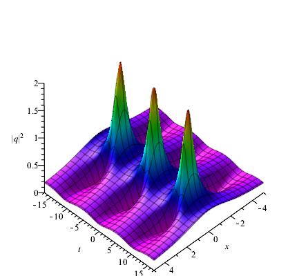
((a)) $a=\xi=0,c=\frac{2}{5},\eta=\frac{1}{2},\gamma_{1}=0$

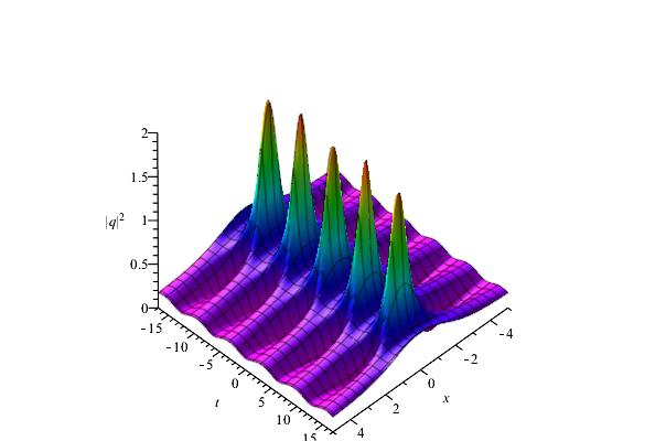
((b)) $a=\xi=0,c=\frac{2}{5},\eta=\frac{1}{2},\gamma_{1}=\frac{1}{2}$

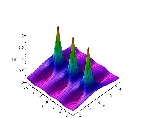
((c)) $a=\xi=0,c=\frac{2}{5},\eta=\frac{1}{2},\gamma_{1}=1$

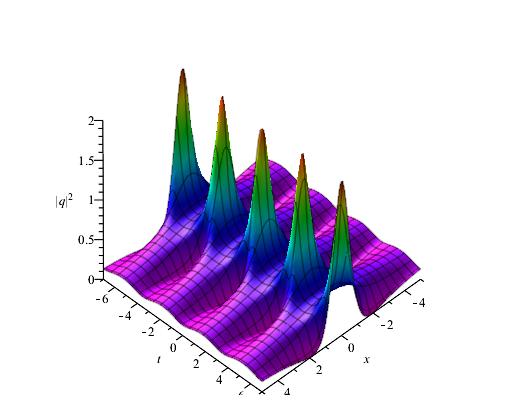
((d)) $a=\xi=0,c=\frac{2}{5},\eta=\frac{1}{2},\gamma_{1}=\frac{3}{2}$

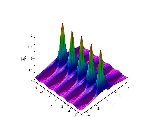
((e)) $a=\xi=0,c=\frac{2}{5},\eta=\frac{1}{2},\gamma_{1}=2$

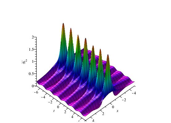
((f)) $a=\xi=0,c=\frac{2}{5},\eta=\frac{1}{2},\gamma_{1}=3$

Figure 1: (Color online) The dynamical evolution of the first-order breather $|q^{[1]}|^{2}$ on the ($x,t$) plane. When the value of $\gamma_{1}$ increases, the number of peaks on same interval of time also increases.

which is the height of peaks of this breather. Obviously, the height is independent of $a,\xi$ and $\gamma_{1}$. This does not mean that $\gamma_{1}$ cannot affect the properties of the breather. In fact, we can see from Eq. (7) that $\gamma_{1}$ actually controls the period of the breather. This observation can be clearly seen in Fig. 1: the number of peaks on same time interval is increasing when $\gamma_{1}$ goes up from $0$ to $3$ with a constant gap $0.5$ (we skip the figure for $\gamma_{1}=\frac{5}{2}$ ) . These pictures clearly show that the resulting breather is compressed by the higher-order effects due to the presence of $\gamma_{1}$ than $\gamma_{1}=0$ case. In addition to the above, when the value of $\gamma_{1}$ increases, the number of peaks also increases. We use a short interval in Fig. 1(a) and 1(b) to avoid too many peaks in it.

Now we can consider what will happen in a breather when its period goes to infinity. According to the explicit expression in Eq. (7) of the first-order breather, this limit can be realized by setting $\displaystyle\lambda=\xi+i\eta\rightarrow\lambda_{0}=-\frac{a}{2}+ic$; i.e., $\lim_{\lambda\rightarrow\lambda_{0}}{q^{[1]}}$. For simplicity, on setting $a=0$ , the limit of the breather solution is obtained as

$$q^{[1]}_{limit}=\left(\frac{4(1+iT)}{X^{2}+T^{2}+1}-1\right)c{{\rm e}^{i2{c}^{2}\left(3\,\gamma_{{1}}{c}^{2}+1\right)t}},$$ (8)

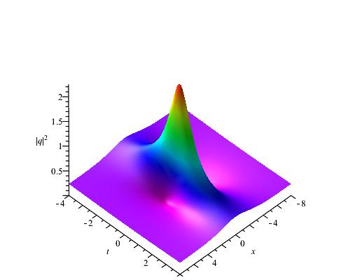
((a)) $c=\frac{1}{2},\gamma_{1}=0$

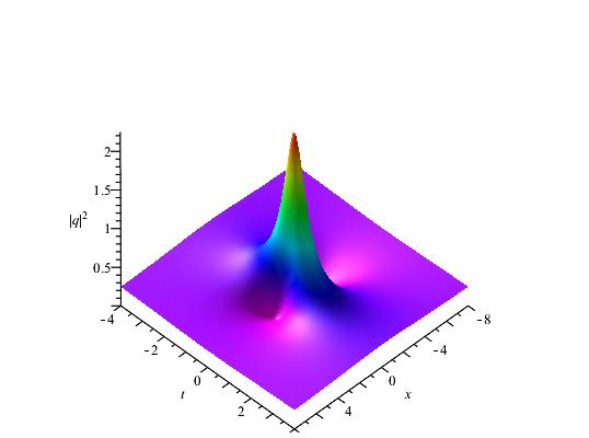
((b)) $c=\frac{1}{2},\gamma_{1}=\frac{1}{2}$

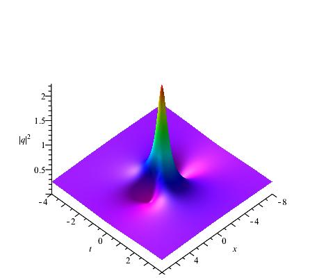
((c)) $c=\frac{1}{2},\gamma_{1}=1$

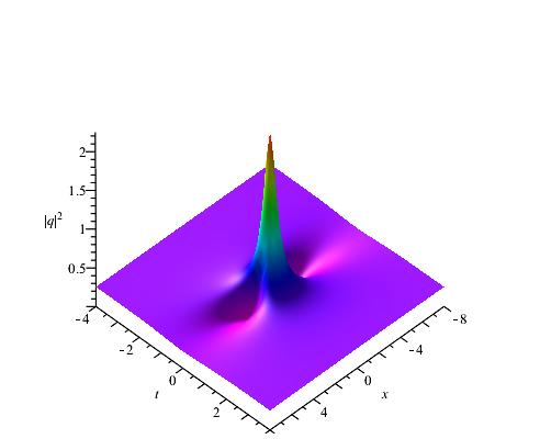
((d)) $c=\frac{1}{2},\gamma_{1}=2$

Figure 2: (Color online) The dynamical evolution of the first-order rogue wave $|q^{[1]}_{limit}|^{2}$ on the ($x,t$) plane. For larger values of $\gamma_{1}$, it is clear that the compression effects in $t$ direction are quite high.

with $T=4\left(1+6\,\gamma_{{1}}{c}^{2}\right){c}^{2}t,\quad X=2cx$. This is nothing but a first-order rogue wave possessing asymptotic height $1$ when $x$ and $t$ go to infinity. Further, we find $|q^{[1]}_{limit}|_{max}^{2}(0,0)=9c^{2}$, which denotes the height of a first-order RW. We can see from $T$ that, like in the case of breather compression, $\gamma_{1}$ is also responsible for compression effect of RW in the time direction, which is clearly seen in Fig. 2 with $\gamma_{1}=0,0.5,1,2$, respectively.

IV Higher-order Rogue Waves

The limit method in Eq. (8) is not applicable for the higher-order breather when $\lambda_{i}\rightarrow\lambda_{0}(i\geq 2)$. We can overcome this problem by using the coefficient of the Taylor expansion in the determinant representation of a higher-order breather $q^{[n]}$ hezhangwangpf2012 ; Hedeterminant . Similar to the case of NLS hezhangwangpf2012 , the first-order rogue wave of GNLSE is given by

$$q^{[1]}_{rw}=\left(\frac{F_{1}+iG_{1}}{H_{1}}-1\right)c{{\rm e}^{i\rho}}.$$ (9)

Here, $F_{1}=4,\quad G_{1}=16\left(1+6\,\gamma_{{1}}{c}^{2}-6\,{a}^{2}\gamma_{{1}}\right){c}^{2}t,$

$$\begin{split}H_{1}=&4\,{c}^{2}{x}^{2}+\left(32\,{c}^{2}\gamma_{{1}}{a}^{3}-16\,{c}^{2}\left(1+12\,\gamma_{{1}}{c}^{2}\right)a\right)xt+(64\,{c}^{2}{\gamma_{{1}}}^{2}{a}^{6}\\ &-64\,{c}^{2}\gamma_{{1}}\left(1+3\,\gamma_{{1}}{c}^{2}\right){a}^{4}+16\,{c}^{2}\left(1+12\,\gamma_{{1}}{c}^{2}+72\,{c}^{4}{\gamma_{{1}}}^{2}\right){a}^{2}\\ &+16\,{c}^{4}\left(6\,\gamma_{{1}}{c}^{2}+1\right)^{2}){t}^{2}+1.\end{split}$$

Note that $q^{[1]}_{rw}$ reduces to the $q^{[1]}_{limit}$ when $a=0$.

What follows is the second-order rogue wave given by the Taylor expansion when $\lambda_{i}\rightarrow\lambda_{0}(i=1,3)$ as the case of NLS hezhangwangpf2012 . There are two patterns for the second-order RW. The first one is called the fundamental pattern possessing a highest peak surrounded by four small equal peaks in two sides. Setting $a=0,s_{1}=0$, then the Taylor expansion in the determinant of $q^{[2]}$ provides

$$q^{[2]}_{rw}=\left(\frac{12(F_{2}+iG_{2})}{H_{2}}-1\right)c{{\rm e}^{i2{c}^{2}\left(3\,\gamma_{{1}}{c}^{2}+1\right)t}}.$$ (10)

Here,

$$\begin{split}F_{2}=&5\,{T}^{4}+\left(6\,{X}^{2}+34\right){T}^{2}-64\,Tt{c}^{2}+{X}^{4}+6\,{X}^{2}-3,\\ G_{2}=&{T}^{5}+\left(2\,{X}^{2}+10\right){T}^{3}-32\,t{c}^{2}{T}^{2}+\left({X}^{4}-14\,{X}^{2}-23\right)T+32\,t{c}^{2}\left({X}^{2}+1\right),\\ H_{2}=&{T}^{6}+\left(3\,{X}^{2}+43\right){T}^{4}-64\,t{c}^{2}{T}^{3}+\left(3\,{X}^{4}-66\,{X}^{2}+307\right){T}^{2}\\ &+\left(192\,{c}^{2}t{X}^{2}-1088\,t{c}^{2}\right)T+1024\,{c}^{4}{t}^{2}+{X}^{6}+3\,{X}^{4}+27\,{X}^{2}+9,\end{split}$$

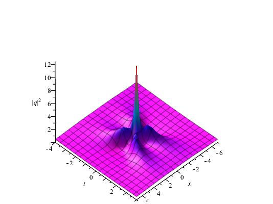
((b)) $a=s_{1}=0,c=\frac{1}{\sqrt{2}},\gamma_{1}=0$

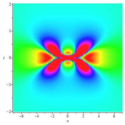
((c)) $a=s_{1}=0,c=\frac{1}{\sqrt{2}},\gamma_{1}=1$

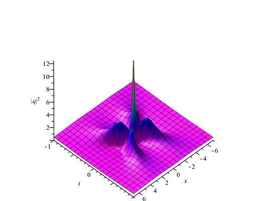
((d)) $a=s_{1}=0,c=\frac{1}{\sqrt{2}},\gamma_{1}=1$

Figure 3: (Color online) The dynamical evolution of the second-order rogue wave $|q^{[2]}_{rw}|^{2}$ on the ($x,t$) plane. Comparing (a) and (b) with (c) and (d) indicates effective high compression in the $t$ direction.

and $X,T$ are defined in Eq. (8). By comparing two cases with $\gamma_{1}=0$ and $\gamma_{1}=1$ in Figure 3, the compression effect in $t$ direction is shown clearly. The second is a triangular pattern, which consists of three equal peaks. Setting $s_{2}=0$,$a=0,s_{1}=50-50i$, then an explicit formula of this pattern is

$$q^{[2]}_{rwtrig}=\left(1-\frac{12(F_{2trig}+iG_{2trig})}{H_{2trig}}\right)c{{\rm e}^{i2{c}^{2}\left(3\,\gamma_{{1}}{c}^{2}+1\right)t}},$$ (11)

with

$$F_{2trig}= 5\,{T}^{4}+\left(24\,\left(1+6\,\gamma_{{1}}{c}^{2}\right)t{c}^{2}{X}^{2}+24\,\left(34\,\gamma_{{1}}{c}^{2}+3\right)t{c}^{2}+1200\,{c}^{2}\right)T$$

$$-3+1200\,{c}^{2}X+6\,{X}^{2}+{X}^{4},$$

$$G_{2trig}= {T}^{5}+\left(8\,\left(1+6\,\gamma_{{1}}{c}^{2}\right)t{c}^{2}{X}^{2}+8\,\left(1+30\,\gamma_{{1}}{c}^{2}\right)t{c}^{2}+600\,{c}^{2}\right){T}^{2}$$

$$+4\,\left(1+6\,\gamma_{{1}}{c}^{2}\right)t{c}^{2}{X}^{4}+\left(-24\,\left(1+14\,\gamma_{{1}}{c}^{2}\right){c}^{2}t-600\,{c}^{2}\right){X}^{2}$$

$$+4800\,\left(1+6\,\gamma_{{1}}{c}^{2}\right){c}^{4}tX-12\,\left(5+46\,\gamma_{{1}}{c}^{2}\right){c}^{2}t-600\,{c}^{2},$$

$$H_{2trig}= {T}^{6}+3\,{X}^{2}{T}^{4}+\left(12\,\left(86\,\gamma_{{1}}{c}^{2}+9\right)t{c}^{2}+1200\,{c}^{2}\right){T}^{3}$$

$$+\left(3\,{X}^{4}+3600\,{c}^{2}X\right){T}^{2}-\left(3600\,{c}^{2}+72\,\left(22\,\gamma_{{1}}{c}^{2}+1\right)t{c}^{2}\right){X}^{2}T$$

$$+{X}^{6}+3\,{X}^{4}+27\,{X}^{2}+14400\,{c}^{4}\left(34\,\gamma_{{1}}{c}^{2}+3\right)t$$

$$+144\,\left(11+228\,\gamma_{{1}}{c}^{2}+1228\,{\gamma_{{1}}}^{2}{c}^{4}\right){t}^{2}{c}^{4}+720000\,{c}^{4}$$

$$-1200\,{X}^{3}{c}^{2}+3600\,{c}^{2}X+9,$$

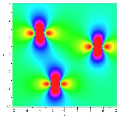
((a)) $a=0,c=\frac{1}{\sqrt{2}},s_{1}=50-50i,\gamma_{1}=0$

((b)) $a=0,c=\frac{1}{\sqrt{2}},s_{1}=50-50i,\gamma_{1}=0$

((c)) $a=0,c=\frac{1}{\sqrt{2}},s_{1}=50-50i,\gamma_{1}=\frac{1}{4}$

((d)) $a=0,c=\frac{1}{\sqrt{2}},s_{1}=50-50i,\gamma_{1}=\frac{3}{4}$

Figure 4: (Color online) The dynamical evolution of the second-order rogue wave $|q^{[2]}_{rwtrig}|^{2}$ on the ($x,t$) plane. It is shown from (b),(c), and (d) that rogue wave compression increases as the value of $\gamma_{1}$ increases.

and X,T are defined in Eq. (8). Figure 4 is plotted for the $|q^{[2]}_{rwtrig}|^{2}$ to show its compression effect. Because of the explicit appearance of $t$ in $F_{2},G_{2},H_{2},F_{2trig}$, $G_{2trig},H_{2trig}$, $q^{[2]}_{rw}$, and $q^{[2]}_{rwtrig}$ one is not be able to derive from the corresponding RWs of the NLSE by a mere scalar transformation of $x,t$.

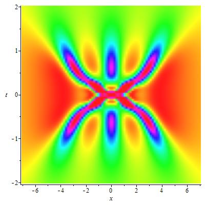
((c)) $a=s_{1}=0,c=\frac{1}{\sqrt{2}},\gamma_{1}=\frac{1}{4}$

Figure 5: (Color online) The dynamical evolution of the third-order rogue wave $|q^{[3]}_{rw}|^{2}$ on the ($x,t$) plane. By comparison with (a) and (b), (c) and (d) are highly compressed.

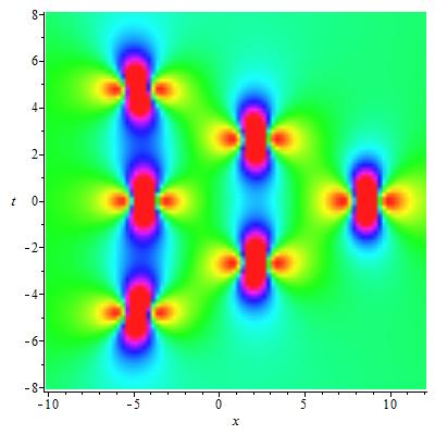
((a)) $c=\frac{1}{\sqrt{2}},s_{1}=-50i,\gamma_{1}=0$

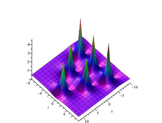
((b)) $c=\frac{1}{\sqrt{2}},s_{1}=-50i,\gamma_{1}=0$

((c)) $c=\frac{1}{\sqrt{2}},s_{1}=-50i,\gamma_{1}=\frac{1}{4}$

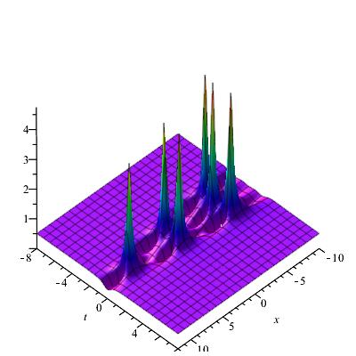
((d)) $c=\frac{1}{\sqrt{2}},s_{1}=-50i,\gamma_{1}=\frac{3}{4}$

Figure 6: (Color online)The dynamical evolution of the third-order rogue wave $|q^{[3]}_{rwtrig}|^{2}$ on the ($x,t$) plane. It is shown from (b), (c), and (d) that rogue wave is compressed more while increasing the value of $\gamma_{1}$.

Next, we construct the third-order RW of GNLSE by substituting present $f_{i}(i=1,2,\cdots,6)$ in $q^{[3]}$ hezhangwangpf2012 . There exists three patterns: a fundamental pattern $q^{[3]}_{rw}$ with $s_{1}=s_{2}=0$, a triangular pattern $q^{[3]}_{rwtrig}$ with $a=s_{2}=0$, and a circular pattern $q^{[3]}_{rwcirc}$ with $a=s_{1}=0$. The explicit form $q^{[3]}_{rw}$ of the fundamental pattern with the third-order RW is given in the Appendix, and, for brevity, the very lengthy forms of the other two cases are deleted. Note that $q^{[3]}_{rw}$ includes the $t$-dependence explicitly. This fact shows that the second-order RW solution cannot be obtained from the corresponding solution of the NLS equation by a scalar transformation of $x,t$. Furthermore, to show the compression effect on the RWs, Figs. (5(c)-7(c)) are plotted for different parametric choices.

V Conclusions

In this paper, we considered the integrable version of the generalized nonlinear Schrödinger equation with several higher-order nonlinear terms, which describes ultra short pulse propagation through nonlinear silica fiber and soliton-type nonlinear excitations in classical Heisenberg spin chain. Using Daurboux transformation and periodic seed solutions, we have constructed the first-order breather solution and also discussed the behavior of these solutions with an infinitely large period. Finally, we have also constructed the first-order, second-order and third-order rogue wave solutions by the Taylor expansion. All of these solutions have parameter $\gamma_{1}$ denoting the contribution of higher-order nonlinear terms. The compressed effects of these solutions are discussed through numerical plots by increasing the value of $\gamma_{1}$. This new phenomenon of the rogue wave is useful for us to observe or analyze its evolution in some complicated physical system. Another advantage of our results of this paper is that, as GNLSE is equivalent to spin chain, the rogue wave nature of spin systems can also be explained through suitable geometrical and gauge equivalence methods. In addition, as higher-order linear and nonlinear effects in optical fibers are playing key roles in explaining the generation and propagation of ultra short pulse through silica wave guides, we hope that our results with all these higher-order effects can be observed in real experiments in the near future.

Appendix: THE THIRD-ORDER ROGUE WAVE

$$q^{[3]}_{rw}=\left(\frac{24(F_{3}+iG_{3})}{H_{3}}+1\right)c{{\rm e}^{2\,i{c}^{2}\left(3\,\gamma_{{1}}{c}^{2}+1\right)t}}$$

$$F_{3}= 11\,{T}^{10}+45\,{X}^{2}{T}^{8}+180\,\left(130\,\gamma_{{1}}{c}^{2}+11\right)t{c}^{2}{T}^{7}+\left(70\,{X}^{4}+420\,{X}^{2}\right){T}^{6}$$

$$+\left(50\,{X}^{6}+480\,\left(15300\,{\gamma_{{1}}}^{2}{c}^{4}+2508\,\gamma_{{1}}{c}^{2}+73\right){t}^{2}{c}^{4}\right){T}^{4}-600\,\left(38\,\gamma_{{1}}{c}^{2}+1\right)t{c}^{2}{X}^{4}{T}^{3}$$

$$+\left(15\,{X}^{8}+7200\,\left(2460\,{\gamma_{{1}}}^{2}{c}^{4}+308\,\gamma_{{1}}{c}^{2}+15\right){t}^{2}{c}^{4}{X}^{2}\right){T}^{2}$$

$$+\left(-240\,\left(38\,\gamma_{{1}}{c}^{2}+1\right)t{c}^{2}{X}^{6}-28800\,\left(4056\,{c}^{6}{\gamma_{{1}}}^{3}+17+300\,{\gamma_{{1}}}^{2}{c}^{4}+210\,\gamma_{{1}}{c}^{2}\right){t}^{3}{c}^{6}\right)T$$

$$+{X}^{10}+15\,{X}^{8}+210\,{X}^{6}+\left(-7200\,\left(220\,{\gamma_{{1}}}^{2}{c}^{4}+20\,\gamma_{{1}}{c}^{2}-1\right){t}^{2}{c}^{4}-450\right){X}^{4}$$

$$+\left(-43200\,\left(628\,{\gamma_{{1}}}^{2}{c}^{4}+124\,\gamma_{{1}}{c}^{2}+5\right){t}^{2}{c}^{4}-675\right){X}^{2}+675$$

$$+10800\,\left(2452\,{\gamma_{{1}}}^{2}{c}^{4}+28\,\gamma_{{1}}{c}^{2}-3\right){t}^{2}{c}^{4}$$

$$G_{3}= {T}^{11}+5\,{X}^{2}{T}^{9}+20\,\left(102\,\gamma_{{1}}{c}^{2}+5\right)t{c}^{2}{T}^{8}+\left(10\,{X}^{4}-60\,{X}^{2}\right){T}^{7}$$

$$+\left(10\,{X}^{6}+480\,\left(12\,{\gamma_{{1}}}^{2}{c}^{4}-268\,\gamma_{{1}}{c}^{2}-29\right){t}^{2}{c}^{4}\right){T}^{5}-120\,\left(82\,\gamma_{{1}}{c}^{2}+7\right)t{c}^{2}{X}^{4}{T}^{4}$$

$$+\left(5\,{X}^{8}+1440\,\left(4524\,{\gamma_{{1}}}^{2}{c}^{4}+548\,\gamma_{{1}}{c}^{2}+19\right){t}^{2}{c}^{4}{X}^{2}\right){T}^{3}+\big{(}-80\,\left(90\,\gamma_{{1}}{c}^{2}+7\right)t{c}^{2}{X}^{6}$$

$$-5760\,\left(99432\,{c}^{6}{\gamma_{{1}}}^{3}+28676\,{\gamma_{{1}}}^{2}{c}^{4}+3086\,\gamma_{{1}}{c}^{2}+107\right){t}^{3}{c}^{6}\big{)}{T}^{2}$$

$$+\left(-7200\,\left(14\,\gamma_{{1}}{c}^{2}+1\right)^{2}{t}^{2}{c}^{4}{X}^{4}+{X}^{10}\right)T-60\,\left(14\,\gamma_{{1}}{c}^{2}+1\right)t{c}^{2}{X}^{8}$$

$$+120\,\left(2\,\gamma_{{1}}{c}^{2}-5\right)t{c}^{2}{X}^{6}-1800\,\left(10\,\gamma_{{1}}{c}^{2}+3\right)t{c}^{2}{X}^{4}$$

$$+\left(57600\,\left(-126\,\gamma_{{1}}{c}^{2}+1176\,{c}^{6}{\gamma_{{1}}}^{3}-564\,{\gamma_{{1}}}^{2}{c}^{4}-7\right){t}^{3}{c}^{6}+2700\,\left(170\,\gamma_{{1}}{c}^{2}+7\right)t{c}^{2}\right){X}^{2}$$

$$+18900\,\left(14\,\gamma_{{1}}{c}^{2}+1\right)t{c}^{2}-14400\,\left(11+1254\,\gamma_{{1}}{c}^{2}+18084\,{\gamma_{{1}}}^{2}{c}^{4}+84168\,{c}^{6}{\gamma_{{1}}}^{3}\right){t}^{3}{c}^{6}$$

$$H_{3}= {T}^{12}+6\,{X}^{2}{T}^{10}+24\,\left(206\,\gamma_{{1}}{c}^{2}+21\right)t{c}^{2}{T}^{9}+\left(15\,{X}^{4}+270\,{X}^{2}\right){T}^{8}$$

$$+\left(20\,{X}^{6}+720\,\left(7596\,{\gamma_{{1}}}^{2}{c}^{4}+1636\,\gamma_{{1}}{c}^{2}+83\right){t}^{2}{c}^{4}\right){T}^{6}-240\,\left(42\,\gamma_{{1}}{c}^{2}-1\right)t{c}^{2}{X}^{4}{T}^{5}$$

$$+\left(15\,{X}^{8}+8640\,\left(3012\,{\gamma_{{1}}}^{2}{c}^{4}+492\,\gamma_{{1}}{c}^{2}+25\right){t}^{2}{c}^{4}{X}^{2}\right){T}^{4}$$

$$+\left(-240\,\left(82\,\gamma_{{1}}{c}^{2}+3\right)t{c}^{2}{X}^{6}-57600\,\left(3048\,{c}^{6}{\gamma_{{1}}}^{3}-2604\,{\gamma_{{1}}}^{2}{c}^{4}-450\,\gamma_{{1}}{c}^{2}-17\right){t}^{3}{c}^{6}\right){T}^{3}$$

$$+\left(6\,{X}^{10}-21600\,\left(548\,{\gamma_{{1}}}^{2}{c}^{4}+76\,\gamma_{{1}}{c}^{2}+1\right){t}^{2}{c}^{4}{X}^{4}\right){T}^{2}$$

$$+\big{(}172800\,\left(46968\,{c}^{6}{\gamma_{{1}}}^{3}+11196\,{\gamma_{{1}}}^{2}{c}^{4}+906\,\gamma_{{1}}{c}^{2}+29\right){t}^{3}{c}^{6}{X}^{2}$$

$$-360\,\left(22\,\gamma_{{1}}{c}^{2}+1\right)t{c}^{2}{X}^{8}\big{)}T$$

$$+{X}^{12}+6\,{X}^{10}+135\,{X}^{8}+\left(2880\,\left(1324\,{\gamma_{{1}}}^{2}{c}^{4}+164\,\gamma_{{1}}{c}^{2}+3\right){t}^{2}{c}^{4}+2340\right){X}^{6}$$

$$+\left(-43200\,\left(428\,{\gamma_{{1}}}^{2}{c}^{4}-12\,\gamma_{{1}}{c}^{2}-5\right){t}^{2}{c}^{4}+3375\right){X}^{4}$$

$$+\left(-64800\,\left(2500\,{\gamma_{{1}}}^{2}{c}^{4}+492\,\gamma_{{1}}{c}^{2}+9\right){t}^{2}{c}^{4}+12150\right){X}^{2}+2025$$

$$+64800\,\left(7260\,{\gamma_{{1}}}^{2}{c}^{4}+772\,\gamma_{{1}}{c}^{2}+23\right){t}^{2}{c}^{4}$$

$$+172800\,\left(213+8056\,\gamma_{{1}}{c}^{2}+720096\,{c}^{6}{\gamma_{{1}}}^{3}+115128\,{\gamma_{{1}}}^{2}{c}^{4}+1836624\,{\gamma_{{1}}}^{4}{c}^{8}\right){t}^{4}{c}^{8}$$

((a)) $a=s_{1}=0,c=\frac{1}{\sqrt{2}},\gamma_{1}=0$

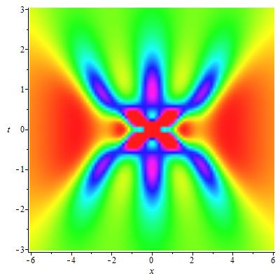
((a)) $a=s_{1}=0,c=\frac{1}{\sqrt{2}},\gamma_{1}=0$

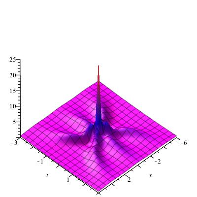
((b)) $a=s_{1}=0,c=\frac{1}{\sqrt{2}},\gamma_{1}=0$

         

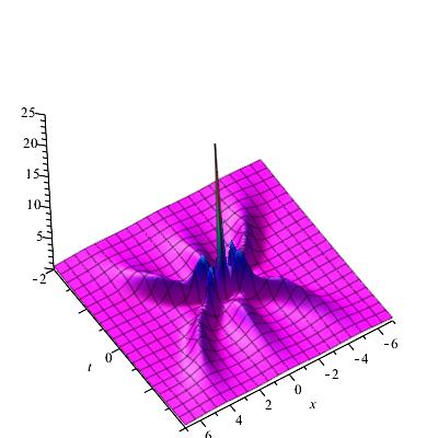
((d)) $a=s_{1}=0,c=\frac{1}{\sqrt{2}},\gamma_{1}=\frac{1}{4}$

((a)) $a=0,c=\frac{1}{\sqrt{2}},s_{2}=5000i,\gamma_{1}=0$

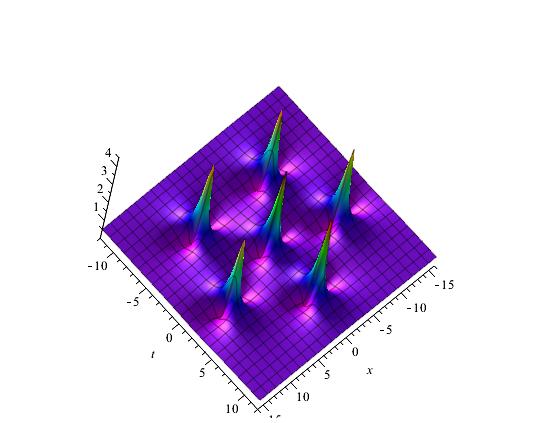
((b)) $a=0,c=\frac{1}{\sqrt{2}},s_{2}=5000i,\gamma_{1}=0$

((c)) $a=0,c=\frac{1}{\sqrt{2}},s_{2}=5000i,\gamma_{1}=\frac{1}{4}$

Figure 7: (Color online) The dynamical evolution of the third-order rogue wave $|q^{[3]}_{rwcirc}|^{2}$ on the ($x,t$) plane. It is shown from (b), (c), and (d) that rogue wave is changing its shape and also compression increases by increasing the value of $\gamma_{1}$.

         

((d)) $a=0,c=\frac{1}{\sqrt{2}},s_{2}=5000i,\gamma_{1}=1$

References

- (1) G. P. Agrawal, Nonlinear Fiber Optics, (Academic Press, San Diego 2006).
- (2) A. Hasegawa, M. Matsumoto, Optical solitons in fibers, (Springer-Verlag, Berlin, 2003).
- (3) L.F. Mollenauer, J.P. Gordon, Solitons in Optical Fibers: Fundamentals And Applications, (Academic Press, New York, 2006).
- (4) K. Porsezian and V. C. Kuriakose, Optical Solitons: Theory and Experiment, Lecture Notes in Physics, Vol. 613, (Springer-Verlag, Berlin, February 2003).
- (5) K. Porsezian and V. C. Kuriakose, Solitons in Nonlinear Optics: Advances and Applications, European Journal of Physics-Special Topics, (Springer-Verlag, Berlin 2009).
- (6) J. R. Taylor, Optical Solitons: Theory and Experiment, (Cambridge University Press, Cambridge, 1992).
- (7) F. Abdullaev, S.Darmanyan, P.Khabibullaev, Optical Solitons, (Springer Series in Nonlinear Dynamics, Berlin, 1993).
- (8) F. Abdullaev, Theory of Solitons in Inhomogeneous Media, (John Wiley, New York, 1994).
- (9) Y. S. Kivshar, G.P. Agrawal, Optical Solitons: From Fibres to Photonic Crystals, (Academic Press, San Diego, 2003).
- (10) G. P. Agrawal, Applications of Nonlinear Fibre Optics, 2nd ed., (Academic Press, New York, 2006).
- (11) N. N. Akhmediev and A. Ankiewicz, Solitons, (Chapman Hall, London, 1997).
- (12) D. H. Peregrine, J. Austral. Math. Soc. B 25, 16 (1983).
- (13) N. Akhmediev, A. Ankiewicz, and M. Taki, Phys. Lett. A 373, 675 (2009).
- (14) D. R. Solli, C. Ropers, P.Koonath, and B. Jalali, Nature (London) 450, 1054 (2007).
- (15) D. R. Solli, C. Ropers, and B. Jalali,Phys. Rev. Lett. 101, 233902 (2008).
- (16) J. M. Dudley, G. Genty, and S. Coen, Rev. Mod. Phys. 78, 1135 (2006); J. M. Dudley, G. Genty, F. Dias, B. Kibler, and N. Akhmediev, Opt. Express 17, 21497 (2009).
- (17) A. N. Ganshin, V. B. Efimov, G. V. Kolmakov, L. P. Mezhov-Deglin, and P. V. E. McClintock, Phys. Rev. Lett. 101, 065303 (2008).
- (18) Yu. V. Bludov, V. V. Konotop, and N. Akhmediev, Phys. Rev. A. 80, 033610 (2009).
- (19) M. S. Ruderman, Eur. Phys. J. Special Topics 185, 57 (2010).
- (20) W. M. Moslem, P. K. Shukla, and B. Eliasson, Euro. Phys. Lett. 96, 25002 (2011).
- (21) R. Höhmann, U. Kuh, H.-J. Stockmann, L. Kaplan, and E. J. Heller, Phys. Rev. Lett. 104, 093901 (2010).
- (22) M. Shats, H. Punzmann, andH.Xia,Phys.Rev. Lett. 104, 104503 (2010).
- (23) A. I. Chervanyov, Phys. Rev. E 83, 061801(R) (2011).
- (24) F. T. Arecchi, U. Bortolozzo, A.Montina, and S. Residori, Phys. Rev. Lett. 106, 153901 (2011).
- (25) A. Chabchoub, N. P. Hoffmann, and N. Akhmediev, Phys. Rev. Lett. 106, 204502 (2011).
- (26) A. Chabchoub, N. P. Hoffmann, and N. Akhmediev, J. Geophys. Res. 117, C00J02 (2012).
- (27) B. Kibler, J. Fatome, C. Finot, G. Millot, F. Dias, G. Genty, N. Akhmediev, and J. M. Dudley, Nat. Phys. 6, 790 (2010).
- (28) A. Ankiewicz, J. M. Soto-Crespo, and N. Akhmediev, Phys. Rev. E. 81, 046602 (2010).
- (29) Y. S. Tao and J. S. He, Phys. Rev. E. 85, 026601 (2012).
- (30) G. G. Yang, L. Li, and S. T. Jia, Phys. Rev. E 85, 046608 (2012).
- (31) S. W. Xu, J. S. He, and L. H. Wang, J. Phys. A 44, 305203 (2011).
- (32) S. W. Xu and J. S. He, J. Math. Phys. 53, 063507 (2012).
- (33) J. S. He, S. W. Xu, and K. Porsezian, J. Phys. Soc. Jpn. 81, 124007 (2012).
- (34) J. S. He, S. W. Xu, and K. Porsezian, J. Phys. Soc. Jpn. 81, 033002 (2012).
- (35) C. Z. Li, J. S. He, and K. Porsezian, Phys. Rev. E 87, 012913 (2013).
- (36) U. Bandelow and N. Akhmediev, Phys. Rev. E 86, 026606 (2012).
- (37) A. Ankiewicz, N. Akhmediev, and J. M. Soto-Crespo, Phys. Rev. E 82, 026602 (2010).
- (38) Yu. V. Bludov, V. V. Konotop, and N. Akhmediev, Eur. J. Phys. Special Topics 185, 169 (2010).
- (39) B. L. Guo and L. M. Lin, Chin. Phys. Lett. 28, 110202 (2011).
- (40) D. Meschede, F. Steglich, W. Felsch, H. Maletta, and W. Zinn, Phys. Rev. Lett. 109, 044102 (2012).
- (41) Z. Y. Qin and M. Gu, Phys. Rev. E 86, 036601 (2012).
- (42) A. Ankiewicz, N. Devine, and N. Akhmediev, Phys. Lett. A 373, 3997 (2009).
- (43) M. Taki, A. Mussot, A. Kudlinski, E. Louvergneaux, M. Kolobov, and M. Douay, Phys. Lett. A 374, 691 (2010).
- (44) Z. Y. Yan, Phys. Lett. A. 374, 672 (2010).
- (45) Y. Y. Wang, J. S. He, and Y. S. Li, Commun. Theor. Phys. 56, 995 (2011).
- (46) L.Wen, L. Li, Z. D. Li, S.W. Song, X. F. Zhang, andW.M. Liu, Eur. Phys. J. D 64, 473 (2011).
- (47) S. W. Xu, J. S. He, and L. H. Wang, Europhys. Lett. 97, 30007(2012).
- (48) C. Q. Dai, G. Q. Zhou, and J. F. Zhang, Phys. Rev. E 85, 016603 (2012).
- (49) J. M. Soto-Crespo, Ph. Grelu, and N. Akhmediev, Phys. Rev. E 84, 016604 (2011).
- (50) J. S. He, H. R. Zhang, L. H. Wang, K. Porsezian, and A. S. Fokas, Phys. Rev. E 87, 052914 (2013).
- (51) M. Lakshmanan, K. Porsezian, and M. Daniel, Phys. Lett. A 133, 483 (1988).
- (52) K. Porsezian, M. Daniel, and M. Lakshmanan, J. Math. Phys. 33, 1807 (1992).
- (53) K. Porsezian, Phys. Rev. E 55, 3785 (1997).
- (54) V. B. Matveev and M. A. Salle, Darboux Transformations and Solitons (Springer, Berlin, 1991).
- (55) J. S. He, L. Zhang, Y. Cheng, and Y. S. Li, Sci. China A 12, 1867 (2006).