Magnetic Structure Producing X- and M-Class Solar Flares in Solar Active Region 11158

Abstract

We study the three-dimensional magnetic structure of solar active region 11158, which produced one X-class and several M-class flares on 2011 February 13$-$16. We focus on the magnetic twist in four flare events, M6.6, X2.2, M1.0, and M1.1. The magnetic twist is estimated from the nonlinear force-free field extrapolated from the vector fields obtained from the Helioseismic and Magnetic Imager on board the Solar Dynamic Observatory using magnetohydrodynamic relaxation method developed by Inoue et al. (2011). We found that strongly twisted lines ranging from half-turn to one-turn twist were built up just before the M6.6- and X2.2 flares and disappeared after that. Because most of the twist remaining after these flares was less than half-turn twist, this result suggests that the buildup of magnetic twist over the half-turn twist is a key process in the production of large flares. On the other hand, even though these strong twists were also built up just before the M1.0 and M1.1 flares, most of them remained afterwords. Careful topological analysis before the M1.0 and M1.1 flares shows that the strongly twisted lines were surrounded mostly by the weakly twisted lines formed in accordance with the clockwise motion of the positive sunspot, whose footpoints are rooted in strong magnetic flux regions. These results imply that these weakly twisted lines might suppress the activity of the strongly twisted lines in the last two M-class flares.

1 Introduction

Solar active phenomena, observed as solar flares, coronal mass ejection (CMEs), and filament eruptions, are driven by the release of magnetic energy in the solar corona (Priest & Forbes 2002). Although many theoretical and numerical models of the magnetic field dynamics have been proposed to date (e.g., Chen 2011; Shibata & Magara 2011), consensus has not yet been reached. On one hand, the optical observations of the magnetic field using the Zeeman effect are limited on the photosphere, therefore it is very difficult to understand the complexity of the three-dimensional (3D) magnetic structure in the solar corona as well as its physical properties and dynamics.

On the other hand, the solar corona has been known to be in the low plasma $\beta$ condition ($\beta$ $\approx$ 10^-2 $\sim$ 10^-1), which means that the force-free condition is approximately satisfied (Gary 2001). Consequently, the nonlinear force-free field (NLFFF) extrapolation becomes a an appropriate technique for understanding the 3D magnetic structure (Schrijver et al. 2006; Metcalf et al. 2008; Wiegelmann & Sakurai 2012). The solar physics satellite Hinode (Kosugi et al. 2007) can provide extremely high spatial resolution vector field data with the Solar Optical Telescope (SOT; Tsuneta et al. 2008). For example, Hinode successfully observed the solar active region NOAA 10930, which generated an X3.4 flare, and provide the vector field as time series data covering before and after the flare. NLFFF extrapolation has already been performed using these vector field data. Guo et al. (2008) presented a 3D view of the core field composed of sheared and twisted field lines lying above the polarity inversion line (PIL), and Schrijver et al. (2008) found that a strong current region accumulated in the strongly sheared and twisted field lines before the flare, most of which disappeared after the flare. Jing et al. (2008) clarified the energy variation in the altitude direction during the flare. Inoue et al. (2011), Inoue et al. (2012a) and Inoue et al. (2012b) also determined the 3D NLFFF by using the magnetohydrodynamic (MHD) relaxation method and the time series vector field data. They quantitatively clarified the variation in the twist profile of the magnetic field lines during the flare, which ultimately leads the cause of the flare onset. Thus, the NLFFF begins to clarify the 3D structure and physical properties such as the stability, as well as the evolution of the magnetic field, in the solar active region; ultimately, it can even suggest the dynamics or onset of the flare. Unfortunately, because the temporal resolution of these vector field data is not sufficient for investigating the evolution of the magnetic field, our understanding has not yet reached a phase that yields a consensus.

More recently, the Helioseismic and Magnetic Imager (HMI; Scherrer et al. 2012; Hoeksema 2013 and see also http://hmi.stanford.edu/magnetic/) and Atmospheric Imaging Assembly (AIA; Lemen et al. 2012) on board a new solar physics satellite, Solar Dynamic Observatory (SDO), can provide vector field data and extreme ultraviolet (EUV) images with unprecedented temporal and spatial resolutions. Thus, we will have many chances to analyze the 3D NLFFF with higher accuracy in space and time.

On 2011 February 13$-$16, the solar active region NOAA 11158 produced one X-class flare along with several M-class flares. This active region consisted of bipoles showing strong shear and twist motion, and exhibited coalescence of the same polarities and ultimately cancellation of opposite polarities, along with complicated motion (Jiang et al. 2012). Fortunately, SDO continuously observed vector field data with a cadence of 12 min and a spatial resolution of $\sim$ 0.5” in a wide region (216$\times$216 Mm²), from February 12 to 16. Note that the field of view of HMI/SDO is the full disk. Only the data in the region, (216$\times$216 Mm²), were released at that time by HMI science team. The SOT/Hinode also provided high-resolution vector field data whose field of view is smaller than that of HMI/SDO; therefore, these data must help us to reconstruct the 3D NLFFF with high spatial and temporal resolution.

The profiles of the temporal evolution of the energy density, current helicity or relative helicity estimated from the NLFFF (Wiegelmann et al. 2012) were reported by Jing et al. (2012). They found a bump structure in which the magnetic helicity increased and decreased before the M6.6 and X2.2 flares, whereas the magnetic energy and current helicity increased monotonically before the X2.2 flare. Liu et al. (2012) analyzed the vector field data related to the M6.6 flare that occurred on February 13 and found a specific region close to the PIL in which a rapid increase in the horizontal field was observed during the flare. They suggested that the 3D field line structure obtained from the NLFFF has a shape favorable for tether-cutting reconnection (Moore et al. 2001), which generates small current-carrying loops close to the PIL that might be related to the significant increase in the horizontal field. Wang et al. (2012) analyzed the magnetic field in terms of the 2D vector field and 3D NLFFF related to the X2.2 flare that occurred on February 15. They also found a rapid enhancement of the horizontal field close to the PIL on the photosphere and supported tether-cutting reconnection as the origin of the flare. Sun et al. (2012) also extrapolated the 3D NLFFF based on HMI/SDO data. They showed highly twisted field lines whose value corresponds to 0.9 turn near the axis above the PIL, the profile along the altitude of the magnetic energy, over 50 $\%$ of which is stored below 6 Mm, eventually indicating that the numerically derived field appeared to be more compact after the flare. Furthermore, Sun et al. (2012) explained the non-radial eruption that occurred to the east in terms of the magnetic topology of the field lines obtained from the NLFFF. On the other hand, Cheung & DeRosa (2012) performed a data-driven simulation in which an extrapolated NLFFF was driven by the normal component of the magnetic field and the horizontal electric field derived by solving the inverse problem of the induction equation (Fisher et al. 2010) from HMI/SDO. They successfully reproduced the eruption in the X2.2 flare and, just after it showed a rapid enhancement in the horizontal field on the photosphere. They concluded that this enhancement resulted from relaxation of the arcade field following a magnetic reconnection that produced a flux rope.

Thus, solar active region NOAA 11158 is attractive for studies of solar flares. A wealth of vector field data and EUV images has been provided by the SDO satellite. Nevertheless the conditions of the M- and X-class flares and the differences in magnetic structure in these flare events are not yet clear. The purpose of this study is to clarify them in terms of the magnetic twist and topology obtained from the 3D NLFFF. The rest of this paper is constructed as follows. The numerical method and observational data set we used in this study are described in Section 2. The results and discussion are presented in Sections 3 and 4,respectively. Finally, the conclusion is summarized in Section 5.

2 Numerical Method and Observations

2.1 NLFFF Extrapolation Based on the MHD-Relaxation Method

We numerically extrapolate the 3D coronal magnetic field assuming it as the NLFFF by using the MHD relaxation method developed by Inoue et al. (2011), Inoue et al. (2012a) and Inoue et al. (2012b), which has already been applied to the solar active region NOAA 10930. This method can numerically solve the following equations;

$$\frac{\partial\mbox{\boldmath$v$}}{\partial t}=-(\mbox{\boldmath$v$}\cdot\mbox{\boldmath$\nabla$})\mbox{\boldmath$v$}+\frac{1}{\rho}\mbox{\boldmath$J$}\times\mbox{\boldmath$B$}+\nu\mbox{\boldmath$\nabla$}^{2}\mbox{\boldmath$v$}.$$ (1)

$$\frac{\partial\mbox{\boldmath$B$}}{\partial t}=\mbox{\boldmath$\nabla$}\times(\mbox{\boldmath$v$}\times\mbox{\boldmath$B$}-\eta\mbox{\boldmath$J$})-\mbox{\boldmath$\nabla$}\phi,$$ (2)

$$\mbox{\boldmath$J$}=\mbox{\boldmath$\nabla$}\times\mbox{\boldmath$B$}.$$ (3)

$$\frac{\partial\phi}{\partial t}+c^{2}_{h}\mbox{\boldmath$\nabla$}\cdot\mbox{\boldmath$B$}=-\frac{c^{2}_{h}}{c^{2}_{p}}\phi,$$ (4)

where $B$ is the magnetic flux density, $v$ is the velocity, $J$ is the electric current density, $\rho$ is the pseudo density, and $\phi$ is a scalar potential. The pseudo density is assumed to be proportional to $|\mbox{\boldmath$B$}|$ in order to ease the relaxation by equalizing the Alfven speed in space. The last equation (4) is used to avoid deviation from $\nabla\cdot\mbox{\boldmath$B$}=0$ and was introduced by Dedner et al. (2002).

The length, magnetic field, pseudo density, velocity, time, and electric current density are normalized by $L_{0}$ = 184.32 Mm, $B_{0}$ = 2500 G, $\rho_{0}$ = $|B_{0}|$, $V_{A}\equiv B_{0}/(\mu_{0}\rho_{0})^{1/2}$, where $\mu_{0}$ is the magnetic permeability, whose value corresponds to 4$\pi\times 10^{-7}$ H/m, $\tau_{A}\equiv L_{0}/V_{A}$ and $J_{0}=B_{0}/\mu_{0}L_{0}$, respectively. The non-dimensional viscosity $\nu$ is set as a constant $(1.0\times 10^{-3})$, and the non-dimensional resistivity $\eta$ is given as

$$\eta=\eta_{0}+\eta_{1}\frac{|\mbox{\boldmath$J$}\times\mbox{\boldmath$B$}||\mbox{\boldmath$v$}|^{2}}{\mbox{\boldmath$|B|$}},$$ (5)

where $\eta_{0}$ is a constant specific to each case whose values are shown in Table 1, and $\eta_{1}=1.0\times 10^{-3}$ in non-dimensional units. The second term is introduced to accelerate the relaxation to the force-free field, particularly in the weak field region. The other parameters $c_{h}^{2}$ and $c_{p}^{2}$ are set to the constants 0.04 and 0.1, respectively.

The velocity field is capped at $v_{max}$ so that it does not correspond to a large value. Let us define $v^{*}=|\mbox{\boldmath$v$}|/|\mbox{\boldmath$v$}_{A}|$ and specify that if the value of $v^{*}$ becomes larger than the value of $v_{max}$ given in Table 1, the velocity is modified as follows;

$$\mbox{\boldmath$v$}\Rightarrow\frac{v_{max}}{v^{*}}\mbox{\boldmath$v$}.$$ (6)

An initial condition is given by the potential field extrapolated using the Fourier method from the normal component on the vector field assuming a periodic condition and an exponential decay in the height direction, whose analytical formula can be found in Equation (13.3.4) in Sturrock (1994). First, we calculate the 3D potential field according to the following equation,

$$\mbox{\boldmath$B$}=\Sigma\mbox{\boldmath$b$}_{(m,n)}^{\ast}exp(ik_{m}x+ik_{n}y-|k|z),$$ (7)

where $k_{m}=2\pi m/L_{x}$, $k_{n}=2\pi n/L_{y}$, $|k|=\sqrt{k_{m}^{2}+k_{n}^{2}}$, $m=-n_{x}/2,\cdots,-1,1,\cdots,n_{x}/2$ and $n=-n_{y}/2,\cdots,-1,1,\cdots,n_{y}/2$, respectively. $\mbox{\boldmath$b$}_{(m,n)}^{\ast}$ consists of three components, $b_{x(m,n)}^{\ast}=-ik_{m}b_{z(m,n)}^{\ast}/|k|$, $b_{y(m,n)}^{\ast}=-ik_{n}b_{z(m,n)}^{\ast}/|k|$, and $b_{z(m,n)}^{\ast}$. However, after this method, vector field is slightly deviated from the original one because $\mbox{\boldmath$b$}_{(0,0)}^{\ast}$ (averaged component) was not counted in the process of the inverse Fourier transformation. Therefore, as next step, we calculate the potential field again using the original vector field without removing the $\mbox{\boldmath$b$}_{(0,0)}^{\ast}$ and the lateral and top boundaries of the 3D magnetic field obtained from equation (7). The potential field is obtained from the normal component of the magnetic field at all of the boundaries according to the $\mbox{\boldmath$\nabla$}^{2}\Phi=0$ (where $\mbox{\boldmath$B$}=-\mbox{\boldmath$\nabla$}\Phi$) after total flux conservation $\int B_{n}dS=0$ is satisfied in the entire domain, where $dS$ represents the surface element on all boundaries, and subscript $n$ represents the component normal to the surfaces of the boundaries.

The observed vector field is given as the bottom boundary condition, and the three components of the magnetic field are fixed. However, the observational data conditions cannot perfectly satisfy the induction equation at the end, so the inconsistent boundary condition generates errors related to $\mbox{\boldmath$\nabla$}\cdot\mbox{\boldmath$B$}$ near the boundary area. Equation (4) can reduce these errors dramatically, as shown in Table.1 (see D$=\int|\mbox{\boldmath$\nabla$}\cdot\mbox{\boldmath$B$}|^{2}dV$). On the top and side boundaries, the transverse fields are determined by an induction equation (2) where a perfect conductive wall is assumed ( i.e., the velocity and electric fields are set to zero), while the normal component is kept with at the initial condition to conserve the total flux. Thus, the side and top boundaries deviate from the real situation; therefore, our analysis is limited to closed loops in the central area.

The Runge-Kutta scheme with fourth-order accuracy for the temporal integral and the central finite difference with second-order accuracy for the spatial derivative are applied as the numerical scheme for this calculation. The numerical domain is covered by 184.32 $\times$ 184.32 $\times$ 184.32 ${\rm Mm^{3}}$, whose area is given by a 128 $\times$ 128 $\times$ 128 grid. The vector field given as the boundary condition is obtained by 4 $\times$ 4 binning from the original vector field 512 $\times$ 512. The grid interval corresponds to about 1688 km/pixel i.e., about 2.3”; therefore, we focus on the scale of the field lines connecting the sunspots in the central area of the numerical domain.

2.2 Observation of AR 11158

We analyzed one X-class flare (X2.2) that occurred at around 01:48 UT on 2011 February 15 and M-class flares (M6.6, M1.0, and M1.1) that occurred at around 17:34 UT on February 13, and 01:36 UT and 07:40 UT on February 16, respectively. The GOES X-ray profile is shown in Figure 1(a). The observation of the vector field by HMI/SDO covered this time span, and HMI team has already provided these data, which are projected and remapped to heliographic coordinates with a spatial resolution of $\sim$ 0.5” and a cadence of 12 min (http://jsoc.stanford.edu/jsocwiki/ReleaseNotes). The vector magnetic fields are obtained from the Very Fast Inversion of the Stokes Vector algorithm (Borrero et al. 2011) based on the Milne-Eddington approximation, and the minimum energy method (Metcalf 1994; Leka et al. 2009) was used to solve the 180^∘ ambiguity in the azimuth angle of the magnetic field. The vector fields before each of the four flares are investigated (M6.6, X2.2, M1.0, and M1.1) as shown in Figure 1(b), in which the gray scale represents the distribution of the normal component of the magnetic field ($B_{z}$).

We use the Ca II H 3968 Å images in these flares for comparison with the extrapolated fields. These images were provided by the Broadband Filter Imager on SOT on board Hinode. The fields of view are 188.28” $\times$ 111.58” with a pixel size of 1728 $\times$ 1024 at 17:35:38 UT on February 13, 111.58” $\times$ 111.58” with 1024 $\times$ 1024 at 01:50:18 UT on February 15, 188.28” $\times$ 111.58” with 1728 $\times$ 1024 at 01:40:39 on February 16 and 111.58” $\times$ 111.58” with 1024 $\times$ 1024 at 07:42:13 on February 16. We also used the EUV images at 94 Å at 23:59:28 UT on 2011 February 14 obtained from AIA/SDO, whose view extracted from the full disk image corresponds to the same as that of HMI used in this study.

3 Results

3.1 Reliability of 3D Magnetic Structure in AR 11158

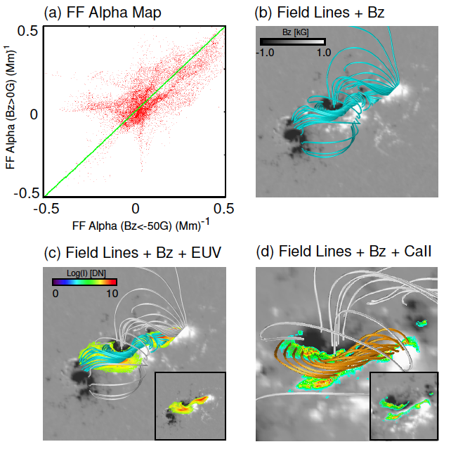
Figure 2: (a) Distribution of force-free $\alpha$ map of reconstructed field at 00:00 UT on February 15. The closed field lines are focused and estimated in the range of about 74 $\times$ 74 ($Mm^{2}$) in the central area. Vertical and horizontal axes represent the values of the force-free $\alpha$ in opposite footpoints on each field line. These values are estimated in the plane at 1688 km above the photosphere, and the field lines are traced from the region in which the values of the magnetic flux are less than $-$50 G. Green line indicates the function of $y=x$. (b) Selected field lines in blue extrapolated from vector field from HMI/SDO observed at 00:00 UT on February 15 plotted over the distribution of the $B_{z}$ component. The field lines are traced from positive polarity values greater than 250 G. (c) EUV images in 94 Å from AIA/SDO observed at 23:59:28 UT on February 14; features whose intensity is more than 1.0$\times 10^{5}$(DN) are plotted over (b). Blue field lines capture the region in which the EUV images are strongly enhanced. Others are plotted in gray. Inset shows the same figure without field lines. (d) Another set of field lines plotted over the $B_{z}$ distribution at the same time as (b)-(c) and Ca II image from SOT/Hinode observed at 01:50:18 UT on February 15. Footpoints of orange field lines are rooted in the region where the Ca II image is strongly enhanced (values greater than 1000(DN)). Inset shows the same figure without field lines.

First, we check the force-freeness of the reconstructed field. As an example, Figure 2(a) shows the force-free $\alpha$ map related to the extrapolated field at 00:00 UT on February 15. The vertical and horizontal axes represent the values of the force-free $\alpha$ estimated on opposite footpoints of each field line. Note that these values are estimated in the plane at 1688 km, i.e., 1 grid size in this case, above the photosphere, and the field lines are traced from the region where $B_{z}<-$50 G. Although the extrapolated field cannot satisfy the force-free condition perfectly because of the deviation from the force-free state in the photosphere, these dotted points seem to be generally distributed along the green line, as shown in our previous result (Inoue et al. 2012a).

Next, we compare the 3D field lines structure with the observational data at the various wavelengths to check its reliability. As an example, Figure 2(b) shows selected 3D magnetic field lines in blue; they are extrapolated from the vector field obtained from HMI/SDO at 00:00 UT on February 15, around 1.5 hr before the X2.2 flare, and plotted over the distribution of the $B_{z}$ component. These selected field lines start from points on the photosphere with $B_{z}>$250G. A strong shear field clearly formed on the PIL between the sunspots located in the center of the plot. This feature is consistent with earlier works (e.g., Sun et al. 2012; Wiegelmann et al. 2012; Jiang & Feng 2013.

The same selected field lines are plotted with blue and gray lines in Figure 2(c) over the distribution of the $B_{z}$ component, and then the brightest part of the AIA’s 94 Å image ($I$ $>$ 1.0$\times 10^{5}$(DN)) is superimposed. The blue lines are arbitrary chosen from the field lines in Figure 2(b) that locate in the strongly enhanced areas of the AIA image. The inset shows the same image without the field lines revealing high-intensity area in the EUV image is not only enhanced near the central area but also extends in the east-west direction; nevertheless, the blue lines can cover these regions.

Figure 2(d) shows the another set of selected field lines in orange and gray plotted over the $B_{z}$ distribution with the Ca II images obtained from FG/Hinode. Only the region with an Ca II signal greater than 1000(DN) observed at 01:50:18 UT on February 15 is drawn in this plot. The inset also shows the same picture without the field lines. The orange field lines correspond to the strong shear field along the PIL with respect to the gray lines, and their footpoints are rooted in the region where the Ca II images are strongly enhanced.

This result is consistent with our previous study (Inoue et al. 2011), which confirms the reliability of the extrapolated field as well as the fact that magnetic reconnection is occurred along these strong non-potential field lines because the strong Ca II illumination is deeply related to magnetic reconnection (Priest & Forbes 2002; Forbes 2000).

3.2 Twist Analysis of the Extrapolated Field in AR 11158

3.2.1 Comparing Magnetic Twist with Ca II Intensity and Distribution

We estimate the magnetic twist from the 3D extrapolated field lines and compare it with the Ca II images obtained from SOT/Hinode in detail. The magnetic twist is an important proxy for determining the stability of the magnetic configuration (Kruskal & Kulsrud 1958; Hood & Priest 1979; Török et al. 2004; Inoue & Kusano 2006) as well as a convenient one for clarifying its topology. The twist index is defined as

$$T_{n}=\int\frac{dT_{n}}{dl}dl=\int\frac{J_{||}}{4\pi B_{||}}dl=\frac{1}{4\pi}\int\alpha dl,$$ (8)

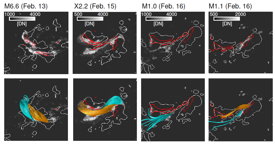
Figure 3: Upper panels show the normal component of magnetic field and twist profile plotted on the Ca II image before the each flare. White lines represent the contours of normal component of magnetic field ($|B_{z}|$=625 G) observed at same times shown in Figure 1(b). Red lines show the magnetic twist ($T_{n}=0.5$) obtained from the NLFFF extrapolated from each vector field. Regions surrounded by red lines are occupied by strongly twisted lines ($T_{n}>0.5$). Gray scale shows Ca II image observed at 17:35:38 UT on February 13, 01:50:18 UT on February 15, 01:40:39 UT and 07:42:13 UT on February 16, respectively. Lower panels show the selected magnetic field lines traced from the regions in which Ca II illuminates strongly. Orange and blue field lines represent twist values more and less than half-turn twist ($T_{n}=0.5$), respectively.

where the line integral $\int dl$ is taken along each magnetic field line, and the force-free $\alpha$ can be obtained from $\alpha=\mbox{\boldmath$J$}\cdot\mbox{\boldmath$B$}/|\mbox{\boldmath$B$}|^{2}$ for each field line. The physical significance is that it represents the degree of twist of a magnetic field line corresponding to the measurement of the magnetic helicity generated by the current parallel to a field line (Berger & Field 1984; Berger & Prior 2006; Török et al. 2010; Inoue et al. 2012b). Note that following the work of Berger & Prior (2006), we applied this definition only to closed loops connecting the sunspots, as shown in Figure 3.

The red lines in the upper panels in Figures 3 represent the contours of half-turn twist ($T_{n}$ = 0.5); i.e., the regions surrounded by the red contours are dominated by strongly twisted lines ($T_{n}>0.5$), with the Ca II images around the peak time of the GOES X-ray flux in each flare. Hereafter, ’strongly twisted lines’ will refer to field lines having more than a half-turn twist ($T_{n}>$0.5). The white lines represent contours of $|B_{z}|=$625 G. The M6.6 and X2.2 flares on February 13 and February 15, respectively, reveal that the locations of strongly twisted regions surrounded by the red lines correspond to enhanced regions of strong Ca II illumination as shown in Figure 2(d). In particular, the profile of the strongly twisted region ($T_{n}>0.5$) at 00:00 UT on February 15 is similar to that of the Ca II image, indicating that the dramatic magnetic reconnection occurred in the strongly twisted magnetic lines having around or more than half-turn twist, as shown in Inoue et al. (2011) and Inoue et al. (2012b). In addition, because the strongly twisted regions on February 15 seem to be larger than that of February 13, this change in the size of the strongly twisted area might be related to the occurrence conditions of X or M-class flares.

On the other hand, the enhancement of the Ca II image in the M1.0 flare on February 16 appears outside the strongly twisted regions. Therefore, the strongly twisted lines seem not to be related to this flare despite the growth in the size of the twisted regions due to the clockwise motion of the positive sunspot. However, in the M1.1 flare, the same regions with strongly twisted lines coincided well with the areas of enhanced Ca II, whose values are smaller than that in the M6.6 or X2.2 flares. At this time, the strongly twisted regions surrounded by the red contours also seem to grow continuously.

The lower panels in Figures 3 show the selected field lines in orange and blue corresponding to magnetic twist of more and less than a half-turn twist, plotted over the upper panels. The footpoints of these field lines lie in the regions where the Ca II image is strongly enhanced; i.e., these field lines connect the two-ribbon flare across the PIL except that in M1.0 flare and weakly twisted lines in M1.1 flare. According to these results, the magnetic field lines on February 15 are obviously elongated compared with those on February 13 and 16, meaning that stronger shear is formed just before the X2.2 flare compared to the M flares.

3.2.2 Temporal Evolution of the Magnetic Twist during the Major Flares

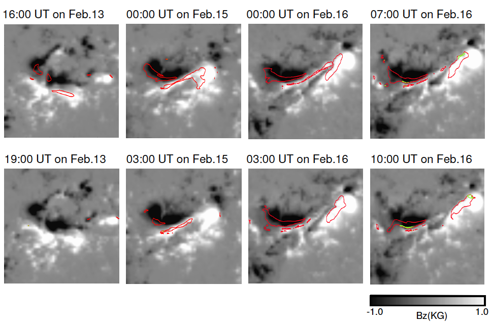
Figure 4: Temporal evolution of the magnetic twist with the distribution of $B_{z}$ component in gray scale, which corresponds to central area of the active region. Upper and lower panels represent 40-90 min before and after each flare (M6.6, X2.2. M1.0, and M1.1) respectively. Red and green lines represent the contours of magnetic twist $T_{n}=0.5$ and $T_{n}=1.0$, respectively. Regions surrounded by red and green lines indicate strongly twisted regions of $T_{n}>0.5$, and $T_{n}>1.0$, respectively.

Figure 4 shows the temporal evolution of the magnetic twist. At 16:00 UT on February 13, the strongly twisted regions in the M6.6 flare, which have 0.5 $<T_{n}<$ 1.0, are already built up by the clockwise motion of the positive sunspot. Most of the strongly twisted lines disappear from the data after this flare. At 00:00 UT on February 15, before the X2.2 flare, the strongly twisted regions are built up again and seem to dominate larger areas than before the previous M6.6 flare. In contrast to the previous flare, some parts of the strongly twisted regions remained even after the X2.2 flare. Nevertheless, the store-and-release scenario of magnetic helicity appeared clearly during the large flares. As a common feature before each flare, we have never found a strongest twisted regions having a value greater than one-turn twist ($T_{n}>$ 1.0). This means that the magnetic configuration is stable against the ideal MHD instability; however, even these magnetic configurations of less than one-turn twist can generate large flares.

The twist profiles at 00:00 UT and 07:00 UT on February 16 are the 40-90 min before the M1.0 and M1.1 flares, respectively. The strongly twisted regions of more than half-turn twist ($T_{n}$ = 0.5) are built up again owing to the continuous clockwise twist and shear motions of the positive sunspot. In contrast to the previous large-scale flares (M6.6 and X2.2), most parts of the strongly twisted regions remained even after these flares. According to the result in Figure 3(c), because the M1.0 flare occurred outside the strongly twisted region, the strongly twisted region seems not to be deeply related to this flare. In other words, these strongly twisted lines remain in the stable state despite their continuing growth. On the other hand, in the M1.1 flare, even stronger twisted regions of more than one turn appear and develop. Nevertheless, all the areas dominated by the strongly twisted lines are weakly illuminated by the Ca II image, as shown in Figure 3(d), and the most strongly twisted regions remained after this flare, as seen in Figure 4. Therefore, this result implies that the strongly twisted lines seem not to be relaxed enough into untwisted lines. These results differ from the common feature of the previous large flares. These topics will be discussed later.

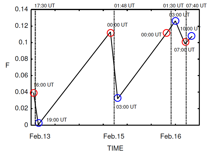
Figure 5: Temporal evolution of the ratio of the fragment of magnetic flux dominated by values of more than half-turn twist to the total magnetic flux from 16:00 UT on February 13 to 10:00 UT on February 16. All flux is estimated in the positive polarity. Vertical dashed lines indicate occurrence of each flare. Red and blue circles indicate time at which each NLFFF was reconstructed before and after each flare, respectively.

In addition to the above analyses, we show the temporal evolution of the ratio of a fragment of the magnetic flux dominated by values of more than half-turn twist to the total flux in Figure 5, whose formula is written by

$$F=\frac{\int_{T_{n}>0.5}B_{z}dS}{\int B_{z}dS},$$ (9)

where the d$S$ is a surface element. These fluxes are estimated due to integrate only those $B_{z}$ in the positive polarities in the same view as in Figure 4. From this result, the M6.6 and X2.2 flares on February 13 and February 15 also clearly exhibit the store-and-release process of the magnetic helicity during the solar flare, and the flux ratio value in the X2.2 event is about three times larger than that of the M6.6 flare. On the other hand, in the last two flares (M1.0 and M1.1 flares), we can see again that the continuous shear and twist motions of the positive sunspot after the large flares regenerate the strongly twisted lines; consequently, a flux comparable to that before the previous large flare is regained. Jing et al. (2012) also indicated that the relative magnetic helicity or helicity injection retain their increasing trend after X2.2 flares. Nevertheless the magnetic flux dominated by the strongly twisted lines is mostly unchanged during the M1.0 and M1.1 flares.

3.2.3 Decrement of the Magnetic Twist during the Major Flares

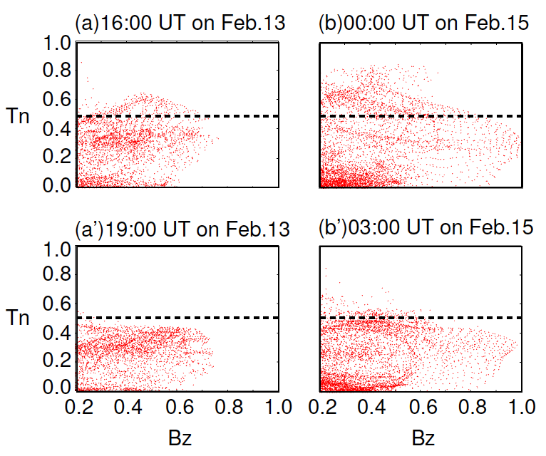
Figure 6: (a),(b) Distribution map related to the twist (vertical axis) and $B_{z}$ components (horizontal axis) at 16:00 UT on February 13 and 00:00 UT on February 15 (before M6.6 and X2.2 flares, respectively). $B_{z}$ component is focused on values in excess of 500G, whose normalized value corresponds to 0.2. Horizontal dashed line indicates the value of half-turn twist($T_{n}=0.5$). (a’), (b’) Maps in same format at 19:00 UT on February 13 and 03:00 UT on February 15 corresponding to the period after the M6.6 and X2.2 flares, respectively.

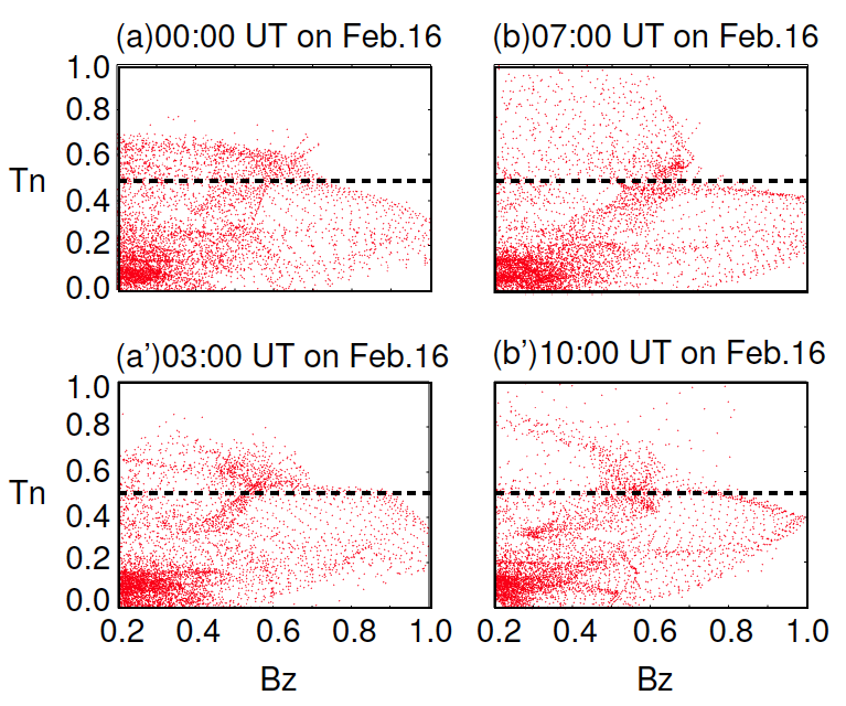
Figure 7: Distribution maps showing magnetic twist value (vertical axis) versus $B_{z}$ component (horizontal axis) before and after M1.0 and M1.1 flares; formats are the same as in Figure 6.

We investigate in more detail about the decrement of the magnetic twist during each flare event to determine how much magnetic twist is needed to cause large flares. Figure 6 shows the distribution map for the values of the magnetic twist (vertical axis) versus the $B_{z}$ component (horizontal axis). We clearly see that most dotted points in the upper area, above the horizontal dotted line, disappear after each flare; thus, the density of the distribution of less than half-turn twist seems to be partially enhanced. This result suggests that the strongly twisted lines (in excess of half-turn twist) relax into less-twisted lines. Because many dotted points are, even after each flare, widely distributed in the twist range $T_{n}<0.5$, the buildup of twisted field lines having more than half-turn twist is an important process for generating the large flares. Moreover, the dotted points above the horizontal dashed line before the X2.2 flare are obviously greater in number and composed of a more twisted region than those before the M6.6 flare, as shown in Figure 5. On the other hand, Figure 7 shows the distribution maps before and after the M1.0 and M1.1 flares. In this case, most of the dotted points remained in the upper region (values greater than half-turn twist) even after the flare and these distributions seem not to change dramatically during these flares, as we expected from the above results.

4 Discussion

The results shown in Section 3 demonstrated that strong (more than a half-turn) magnetic twist is closely related to produce the large flares, i.e., the X2.2 and M6.6 flares, because most of the strong twist disappeared after these two strong flares. On the other hand, the distribution of the magnetic twist did not change dramatically before and after the M1.0 and M1.1 flare events, in which the strongly twisted lines ($T_{n}>0.5$) and even those with more than one-turn twist ($T_{n}>1.0$) were built up before these weak flares. In this section, we investigate the temporal evolution of the twisted field lines and its magnetic topology before each flare to explain why the strongly twisted field lines remained after the M1.0 and M1.1 flares. Eventually, we give a suggestion related to the mechanism of the confined and ejective eruptions.

4.1 Temporal Evolution of the Twisted Field Lines

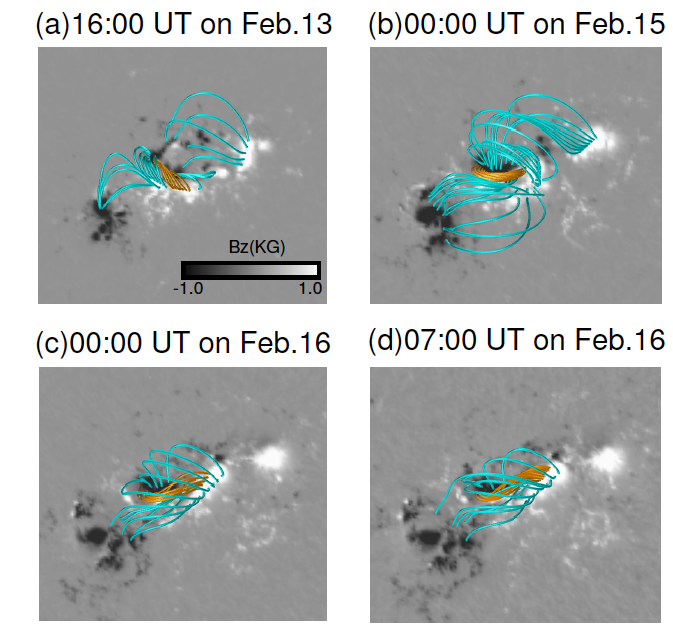
Figure 8: Selected field lines plotted over $B_{z}$ component 40-90 min before each flare. Orange represents twist values of $T_{n}>0.5$; blue corresponds to $T_{n}<0.5$. Both plotted from positive polarities of greater than 250G.

Figure 8 shows selected 3D field lines before each flare. The strongly twisted lines (orange) lie on the neutral line in each case. Although some weakly twisted lines (blue) in addition to the strongly twisted lines also form the shear structure at 16:00 UT on February 13, in the last two flares (M1.0 and M1.1 flares), some field lines whose footpoints are rooted in regions of strong magnetic field seem to surround the strongly twisted lines. These relationships between the strongly ($T_{n}>0.5$) and weakly ($T_{n}<0.5$) twisted field lines, especially those surrounding the strongly twisted lines, might imply some influences on the dynamics of each flare.

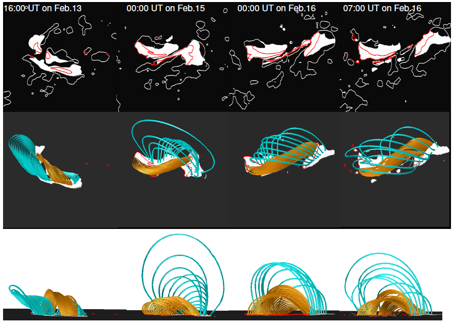
Figure 9: Top panels show the connectivity maps in black and white scale are represented at 40-90 min before each flare. White lines represent the contours of $|B_{z}|=500$ G; red line indicates contour of magnetic twist corresponding to $T_{n}$=0.5. White regions are specific areas in which the footpoints of the closed field lines connecting the regions surrounded by white contours are rooted. In the middle panels, the field lines are plotted over the upper panels except for the white lines. All of their footpoints are rooted in the regions in the white areas. Orange and blue field lines have magnetic twist values greater and less than $T_{n}$=$0.5$, respectively. In the lower panels, side views of 3D field lines.

We investigate in detail the relationship between these strongly and weakly twisted lines before each flare by using the connectivity map in the upper panels in Figure 9, which focuses on specific field lines for which both footpoints are rooted in the regions of the strong magnetic field ($B_{z}>$500G and $B_{z}<-$500G). Consequently, both footpoints of the selected field lines are rooted in the regions shown in white in both polarities, where the white lines correspond to the contour at $|B_{z}|=$500G.

These field lines are shown in the middle panels in Figure 9. According to these results, at 16:00 UT on February 13, all the selected closed field lines form a similar shear structure, which are strongly related to M6.6 flares because Ca II image is strongly illuminating in those footpoints in Figure 3. Afterward, these twisted lines are deformed due to the subsequently strong sheared and twisted motion of the sunspot. Consequently, at 00:00 UT on February 15, the weakly twisted lines (blue) seem to partially cover the strongly twisted lines (orange). In fact, X2.2 flare can be considered to be induced by the strongly twisted lines over the half turn twist from Figure 3. Eventually, on February 16, most of the strongly twisted lines were covered by weakly twisted lines. These results clearly show that the weakly twisted lines, which constituted the core field on February 13, play a role in the overlying field lines surrounding the strongly twisted lines. Therefore, as time passes, the strongly twisted lines seem to fall into an unfavorable condition to escape from the lower coronal region.

In the lower panels in Figure 9, we show a side view of the 3D field lines before each flare in order to more understand the overview profiles of the field lines qualitatively. We clearly see at 00:00 UT on February 15 that the part of the weakly twisted field lines in blue extends to a higher position compared to those on February 13. On the other hand, although these extended loops are still remained at 00:00 UT and 07:00 UT on February 16, they seem to become a bit more compact than earlier. This might be related to the report by Sun et al. (2012), which indicated that this active region decreased in volume after the X2.2 flare.

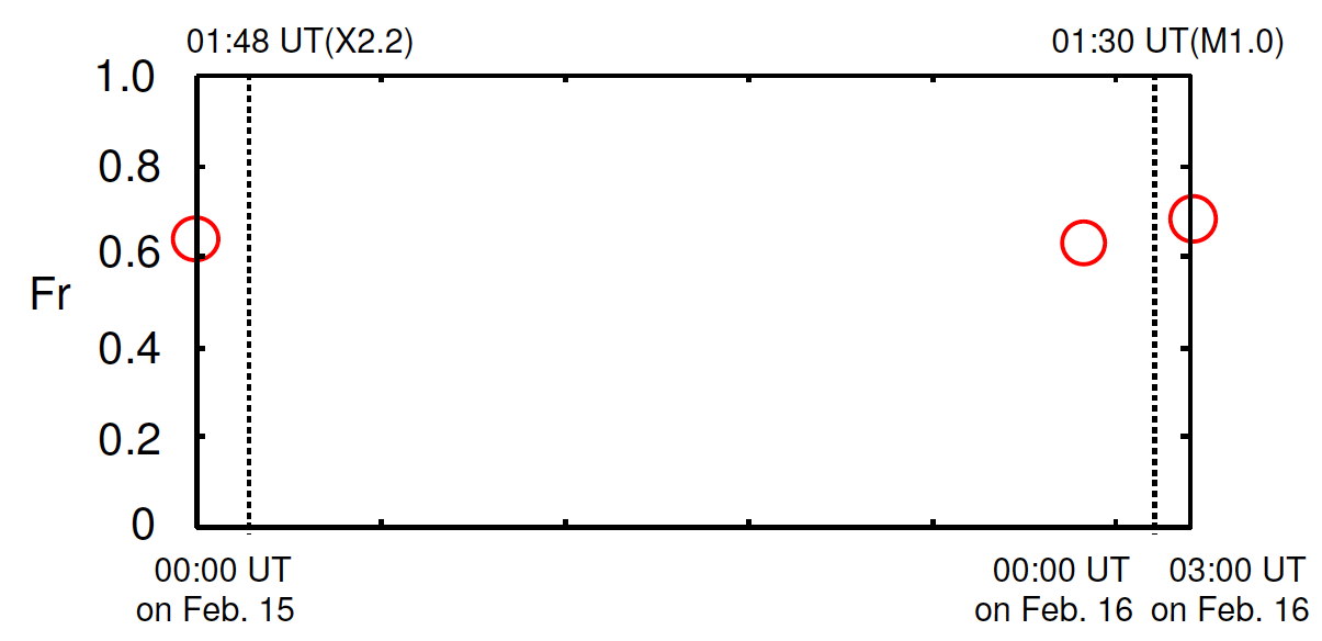
Figure 10: Temporal evolution of the ratio of the fragment of the magnetic flux less than $T_{n}=$0.5 to the total integrated flux. In this case, all of the magnetic flux is estimated by the closed field lines connecting both polarities in white in Figure 9 and integrated only those $B_{z}$ in the positive polarities.

Figure 10 shows the flux ratio of the weakly twisted lines connecting both polarity regions in white in Figure 9 to the magnetic flux related to the entire closed field, which is composed of the strongly and weakly twisted lines connecting same areas. All of the flux values are estimated due to integrate only those $B_{z}$ in the positive polarities before the flares on February 15 and 16, and the flux ratio formula is defined as

$$F_{r}=\frac{\int_{0<T_{n}<0.5}B_{z}dS}{\int B_{z}dS},$$ (10)

where d$S$ is a surface element. Note that because we are interested in the deformed weakly twisted lines due to subsequently strong twisted and sheared motion of the sunspot after M6.6 flare, the value on February 13 is not plotted in Figure 10.

This result shows us that this flux ratio remains 62$\%$-67$\%$ during the three flares. Therefore, these results reveal no large variations in the magnetic flux. Before the X2.2 flare on February 15, even though the weakly twisted lines whose footpoints are both at $|B_{z}|>$500 G had already deformed, they covered the strongly twisted fields only in part. This surrounding condition might allow the escape of the strongly twisted field from the lower coronal region. On the other hand, the magnetic field configuration is changed by the strong shear and twist motions of the sunspot; thus the weakly twisted field lines covered the entire strongly twisted field region on February 16. Furthermore, along with the results in Figure 10, because the ’total’ magnetic energy accumulated in the root of the the weakly twisted lines is superior to that of the strongly twisted field lines, these probably have the potential to confine the dynamics of the strongly twisted field in the M1.0 and M1.1 flares. For example, this confinement indicates the suppression of the exhaustion at the magnetic reconnection site and consequent rapid energy release.

4.2 Overlying Field Lines

In previous subsection, we discuss the magnetic structure inducing the X- and M-class solar flares in terms of the temporal evolution and topologies of the twisted field lines formed in the lower corona. However, the overlying field lines surrounding these twisted lines also play an important role in determining whether CMEs are produced or not even if the twist value in the twisted line is more than one-turn twist (Guo et al. 2010). Therefore, we need to discuss the overlying field lines quantitatively. The decay index is one of quantitative indexes of the overlying fields by estimating how rapidly the strength of the magnetic field decreases with height, which is given by the following equation,

$$n(z)=-\frac{z}{|\mbox{\boldmath$B$}|}\frac{\partial|\mbox{\boldmath$B$}|}{\partial z}.$$

The decay index is often referred to an estimation of a criterion for the torus instability whose threshold lies in the range of 1.1$\leq n_{c}\leq$2, which was introduced by Kliem & Török (2006) and Démoulin & Aulanier (2010). An eruption of the flux rope was numerically confirmed by Török & Kliem (2007), Fan (2010) and Aulanier et al. (2010).

In this study, as mentioned in Section 2, we can discuss only the closed field lines in the central area within a height of around few dozens of Mm due to the problem associated with lateral boundary conditions. Because of this, decay index in the overlying field lines higher than few dozens of Mm is strongly affected by these boundary conditions. Furthermore because decay index cannot be applied to the non-potential field structure retrieved with our mode within a height of around few dozens of Mm, it is difficult to discuss it in the framework of our study. However, Nindos et al. (2012) already calculated the decay index related to the NLFFF (Wiegelmann et al. 2012) in AR11158 in long term period on February 11-16. They showed the long-term temporal evolution of the decay index at each height and concluded that the onset of eruptions does not depend critically on the long-term evolution of the decay index of the background field before CMEs. In other words, this result might support that the temporal evolution of the twisted field lines play an important role in controlling the flares and CMEs in this active region.

In fact, Yashiro et al. (2011) reported that partial Halo and Halo CMEs were observed associated with M6.6 and X2.2 flares, on the other hand, we were not able to observe the CMEs just after M1.0 and M1.1 flares (http://cdaw.gsfc.nasa.gov/CMElist/). Only one CME originated from AR11158 was observed after X2.2-class flare occurred. However, the flare which is source of this CME occurred in the edge of this active region. Therefore these observations might support that flux rope eruption is confined by the weak twisted line plotted in blue in Figure 9 during M1.0 and M1.1 flares.

4.3 Formation of the more strongly twisted Flux Tube before an Eruption

In this study, the strongly twisted field lines before M6.6 and X2.2 flares distribute in $0.5<T_{n}<1.0$, which implies that the magnetic configuration is stable against the MHD instability. Although, these magnetic twists obtained from our study seem to be weak to induce the large flares, this is because the NLFFF approximation omits the necessary physics in a dynamic process. i.e., missing the tether-cutting process. Some authors also have supported tether-cutting reconnection as a feasible process causing eruption in this active region as described in Section 1. Because of conservation of the magnetic helicity, tether-cutting reconnection in the strongly twisted lines generates longer and more strongly twisted field lines just before an eruption. For example, Amari et al. (2010) and Amari et al. (2011) showed the strongly twisted flux tube along the PIL through the tether-curring reconnection in the twisted field lines due to the flux cancellation process or converging flows on the photosphere. Eventually, this flux tube is successfully launched from the lower corona. More recently, Kusano et al. (2012) indicated two types of emerging flux that produce the long strongly twisted field lines in the pre-existing coronal magnetic field through tether-cutting-like reconnection, where the initial pre-existing field is assumed to form uniformly sheared arcades in the linear force-free approximation. They reported that the angle between the emerging flux and the pre-existing shear field lines is important. Thus, tether-cutting process would be feasible of producing large flares even the accumulated twist in the solar active region is less than one-turn twist.

5 Summary

This paper presented the 3D magnetic structures of AR11158, which produced a X-class and several M-class flares on 2011 February 13-16. We focus on four flares, M6.6, X2.2, M1.0, and M1.1, as shown Figure1(a), which are analyzed in terms of the magnetic twist obtained from the NLFFF and its variation before and after each flare. These NLFFFs were obtained from the MHD relaxation method developed by Inoue et al. (2011), Inoue et al. (2012a), and Inoue et al. (2012b). Our previous studies were focused on a X-class flare where we discussed its magnetic structure and physical condition in terms of the magnetic twist in the solar active region 10930. However, in this present study, we are able to compare them quantitatively in the various class-flares occurred in the active region 11158 and eventually gave a suggestion related to the ejective and confined eruptions of CME as well as the occurrence conditions of X- and M-class flares.

First of all, we compared the magnetic twist obtained from the 3D field lines before each flare event with Ca II images obtained from SOT/Hinode. Particularly in the M6.6 and X2.2 flares, we found that the footpoints of the strongly twisted field lines whose values are larger than the half-turn twist (i.e., $T_{n}>0.5$) corresponded to the locations well within the strong enhancement of Ca II, which is consistent with our previous study (Inoue et al. 2011). These results show that dramatic magnetic reconnection occurred in the strongly twisted lines ($T_{n}>0.5$) in these flares. Furthermore, we found that the magnetic flux ratio of the strongly twisted lines to the total flux before the X2.2 flare was about three times larger than that in the M6.6 flare. On the other hand, magnetic twists larger than $T_{n}=1.0$ have never seen in either cases which indicates that the magnetic configuration is stable against the ideal MHD instability. The magnetic twists obtained in this study seem a little weak to produce a large flare but this is due to the limitation of the NLFFF omitting some necessary physics in a dynamics, e.g., tether cutting process is one of them. For instance, although the value of $T_{n}$=0.5 is low for a single flux tube, magnetic reconnection between these twisted lines could produce highly twisted lines having more than a one-turn twist ($T_{n}$ = 1.0) at least; therefore, active regions accumulating the twisted field lines at 0.5$<T_{n}<$1.0 could be capable of producing large flares.

A comparison of the conditions before and after each flare revealed that strongly twisted lines were built up before each flare; they disappeared after the M6.6 and X2.2 flares, whereas the weakly twisted lines ($T_{n}<0.5$) remained. On the other hand, although the strongly twisted lines were also built up before the last two flares on February 16, whose magnetic flux strength was comparable to that of the X2.2 flares, the overall distributions of the magnetic twist did not change dramatically after the flare happening. We carefully investigated the temporal evolution of the twisted lines and their magnetic topologies before these flares. We found that the twisted field lines are deformed due to the strongly sheared and twisted motion of the sunspot, consequently the weakly twisted lines whose footpoints are at $|B_{z}|>$500 G covered the strongly twisted lines before M1.0 and M1.1 flares. Because the CMEs were not observed associated with these flares and temporal evolution of the decay index in the overlying field lines surrounding the twisted field lines were not critically depended on an initiation of eruptions, reported by Nindos et al. (2012), these weakly twisted field lines might confine the activities of the strongly twisted lines even though the magnetic flux of the strongly twisted lines is stronger than that of the lines producing the M6.6 flare and comparable to that of the lines producing the X2.2 flare.

This case is one example of many active regions. Therefore, further analysis of the various solar active regions using observational and numerical approaches is needed to reach on a possible conclusion for flare dynamics. HMI/SDO successfully observed the vector field of AR 11158 with unprecedented spatial and temporal resolution and will provide that data for many active regions. We can expect that the results obtained from these data analyses will enable us to better understand the dynamics of this magnetic activities.

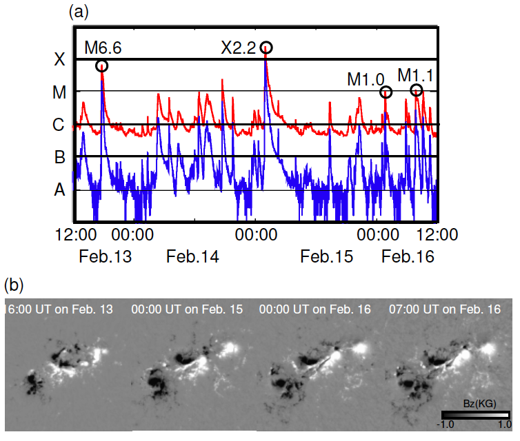
Figure 1: (a) Time profile of X-ray flux measured by GOES satellite on 2011 February 13-16. The solar X-ray outputs in the 1.0-8.0 Å(red) and 0.5-4.0 Å(blue) passband are plotted. The four flares (M6.6, X2.2, M1.0, and M1.1) marked by circles are analyzed in this study. (b) Vector fields 40-90 min before each flare. The distributions of the normal component of the magnetic field($B_{z}$) at each time are plotted in gray scale.

Table 1: Parameters and values of $D=\int|\mbox{\boldmath$\nabla$}\cdot\mbox{\boldmath$B$}|^{2}$dV related to the selected field. The period is from 2011 February 13 to 16.

Time	$\eta_{0}$	$v_{max}$	D
16:00 UT on Feb.13	$2.5\times 10^{-5}$	$2.5\times 10^{-3}$	$2.25\times 10^{-7}$
19:00 UT on Feb.13	$2.5\times 10^{-5}$	$2.5\times 10^{-3}$	$2.41\times 10^{-7}$
00:00 UT on Feb.15	$2.5\times 10^{-5}$	$5.0\times 10^{-3}$	$3.186\times 10^{-7}$
03:00 UT on Feb.15	$2.5\times 10^{-5}$	$2.5\times 10^{-3}$	$2.545\times 10^{-7}$
00:00 UT on Feb.16	$5.0\times 10^{-5}$	$2.5\times 10^{-3}$	$8.518\times 10^{-7}$
03:00 UT on Feb.16	$5.0\times 10^{-5}$	$2.5\times 10^{-3}$	$1.007\times 10^{-6}$
07:00 UT on Feb.16	$5.0\times 10^{-5}$	$5.0\times 10^{-3}$	$7.740\times 10^{-7}$
10:00 UT on Feb.16	$5.0\times 10^{-5}$	$2.5\times 10^{-3}$	$9.676\times 10^{-7}$

References

- Amari et al. (2010) Amari, T., Aly, J.-J., Mikic, Z., & Linker, J. 2010, ApJ, 717, L26
- Amari et al. (2011) Amari, T., Aly, J.-J., Luciani, J.-F., Mikic, Z., & Linker, J. 2011, ApJ, 742, L27
- Aulanier et al. (2010) Aulanier, G., Török, T., Démoulin, P., & DeLuca, E. E. 2010, ApJ, 708, 314
- Berger & Field (1984) Berger, M. A., & Field, G. B. 1984, Journal of Fluid Mechanics, 147, 133
- Berger & Prior (2006) Berger, M. A., & Prior, C. 2006, Journal of Physics A Mathematical General, 39, 8321
- Borrero et al. (2011) Borrero, J. M., Tomczyk, S., Kubo, M., et al. 2011, Sol. Phys., 273, 267
- Chen (2011) Chen, P. F. 2011, Living Reviews in Solar Physics, 8, 1
- Cheung & DeRosa (2012) Cheung, M. C. M., & DeRosa, M. L. 2012, ApJ, 757, 147
- Dedner et al. (2002) Dedner, A., Kemm, F., Kröner, D., et al. 2002, Journal of Computational Physics, 175, 645
- Démoulin & Aulanier (2010) Démoulin, P., & Aulanier, G. 2010, ApJ, 718, 1388
- Fan (2010) Fan, Y. 2010, ApJ, 719, 728
- Fisher et al. (2010) Fisher, G. H., Welsch, B. T., Abbett, W. P., & Bercik, D. J. 2010, ApJ, 715, 242
- Forbes (2000) Forbes, T. G. 2000, J. Geophys. Res., 105, 23153
- Gary (2001) Gary, G. A. 2001, Sol. Phys., 203, 71
- Guo et al. (2008) Guo, Y., Ding, M. D., Wiegelmann, T., & Li, H. 2008, ApJ, 679, 1629
- Guo et al. (2010) Guo, Y., Ding, M. D., Schmieder, B., et al. 2010, ApJ, 725, L38
- Hoeksema (2013) Hoesksema et al. 2012, in preparation for solar physics
- Hood & Priest (1979) Hood, A. W., & Priest, E. R. 1979, Sol. Phys., 64, 303
- Inoue & Kusano (2006) Inoue, S., & Kusano, K. 2006, ApJ, 645, 742
- Inoue et al. (2011) Inoue, S., Kusano, K., Magara, T., Shiota, D., & Yamamoto, T. T. 2011, ApJ, 738, 161
- Inoue et al. (2012a) Inoue, S., Magara, T., Watari, S., & Choe, G. S. 2012, ApJ, 747, 65
- Inoue et al. (2012b) Inoue, S., Shiota, D., Yamamoto, T. T., et al. 2012, ApJ, 760, 17
- Jiang et al. (2012) Jiang, Y., Zheng, R., Yang, J., et al. 2012, ApJ, 744, 50
- Jiang & Feng (2013) Jiang, C., & Feng, X. 2013, arXiv:1304.2979
- Jing et al. (2008) Jing, J., Wiegelmann, T., Suematsu, Y., Kubo, M., & Wang, H. 2008, ApJ, 676, L81
- Jing et al. (2012) Jing, J., Park, S.-H., Liu, C., et al. 2012, ApJ, 752, L9
- Kliem & Török (2006) Kliem, B., Török, T. 2006, Physical Review Letters, 96, 255002
- Kruskal & Kulsrud (1958) Kruskal, M. D., & Kulsrud, R. M. 1958, Physics of Fluids, 1, 265
- Kosugi et al. (2007) Kosugi, T., Matsuzaki, K., Sakao, T., et al. 2007, Sol. Phys., 243, 3
- Kusano et al. (2012) Kusano, K., Bamba, Y., Yamamoto, T. T., et al. 2012, ApJ, 760, 31
- Leka et al. (2009) Leka, K. D., Barnes, G., Crouch, A. D., et al. 2009, Sol. Phys., 260, 83
- Lemen et al. (2012) Lemen, J. R., Title, A. M., Akin, D. J., et al. 2012, Sol. Phys., 275, 17
- Liu et al. (2012) Liu, C., Deng, N., Liu, R., et al. 2012, ApJ, 745, L4
- Metcalf (1994) Metcalf, T. R. 1994, Sol. Phys., 155, 235
- Metcalf et al. (2008) Metcalf, T. R., DeRosa, M. L., Schrijver, C. J., et al. 2008, Sol. Phys., 247, 269
- Moore et al. (2001) Moore, R. L., Sterling, A. C., Hudson, H. S., & Lemen, J. R. 2001, ApJ, 552, 833
- Nindos et al. (2012) Nindos, A., Patsourakos, S., & Wiegelmann, T. 2012, ApJ, 748, L6
- Priest & Forbes (2002) Priest, E. R., & Forbes, T. G. 2002, A&A Rev., 10, 313
- Scherrer et al. (2012) Scherrer, P. H., Schou, J., Bush, R. I., et al. 2012, Sol. Phys., 275, 207
- Schrijver et al. (2006) Schrijver, C. J., DeRosa, M. L., Metcalf, T. R., et al. 2006, Sol. Phys., 235, 161
- Schrijver et al. (2008) Schrijver, C. J., De Rosa, M. L., Metcalf, T., et al. 2008, ApJ, 675, 1637
- Schrijver et al. (2011) Schrijver, C. J., Aulanier, G., Title, A. M., Pariat, E., & Delannée, C. 2011, ApJ, 738, 167
- Shibata & Magara (2011) Shibata, K., & Magara, T. 2011, Living Reviews in Solar Physics, 8, 6
- Sturrock (1994) Sturrock, P. A. 1994, Plasma Physics, Cambridge University Press
- Sun et al. (2012) Sun, X., Hoeksema, J. T., Liu, Y., et al. 2012, ApJ, 748, 77
- Sun et al. (2012) Sun, X., Hoeksema, J. T., Liu, Y., Chen, Q., & Hayashi, K. 2012, ApJ, 757, 149
- Török et al. (2004) Török, T., Kliem, B., & Titov, V. S. 2004, A&A, 413, L27
- Török & Kliem (2007) Török, T., & Kliem, B. 2007, Astronomische Nachrichten, 328, 743
- Török et al. (2010) Török, T., Berger, M. A., & Kliem, B. 2010, A&A, 516, A49
- Tsuneta et al. (2008) Tsuneta, S., Ichimoto, K., Katsukawa, Y., et al. 2008, Sol. Phys., 249, 167
- Wang et al. (2012) Wang, S., Liu, C., Liu, R., et al. 2012, ApJ, 745, L17
- Wiegelmann et al. (2012) Wiegelmann, T., Thalmann, J. K., Inhester, B., et al. 2012, Sol. Phys., 67
- Wiegelmann & Sakurai (2012) Wiegelmann, T., & Sakurai, T. 2012, Living Reviews in Solar Physics, 9, 5
- Yashiro et al. (2011) Yashiro, S., Gopalswamy, N., Akiyama, S., & Makela, P. A. 2011, AGU Fall Meeting Abstracts, 1965