Current-driven homogenization and effective medium parameters for finite samples

Abstract

Reflection and refraction of electromagnetic waves by artificial periodic composites (metamaterials) can be accurately modeled by an effective medium theory only if the boundary of the medium is explicitly taken into account and the two effective parameters of the medium – the index of refraction and the impedance – are correctly determined. Theories that consider infinite periodic composites do not satisfy the above condition. As a result, they cannot model reflection and transmission by finite samples with the desired accuracy and are not useful for design of metamaterial-based devices. As an instructive case in point, we consider the “current-driven” homogenization theory, which has recently gained popularity. We apply this theory to the case of one-dimensional periodic medium wherein both exact and homogenization results can be obtained analytically in closed form. We show that, beyond the well-understood zero-cell limit, the current-driven homogenization result is inconsistent with the exact reflection and transmission characteristics of the slab.

I Introduction

In the past decade, interest in electromagnetic homogenization theories has experienced a remarkable revival, especially when applied to artificial periodic composites (metamaterials) Simovski (2009, 2011). The ultimate goal of any homogenization or effective medium theory (EMT) is to describe reflection and refraction of waves by finite samples. In the case of homogeneous natural materials, an accurate description of this kind is possible only if both the index of refraction and the impedance of the material are known with sufficient precision. Correspondingly, the majority of EMTs attempt to replace a periodic composite sample with a sample of the same overall shape but spatially-uniform effective refractive index and impedance and sharp boundaries, although in some cases Drude transition layers are introduced or considered Simovski (2009). However, when the EMTs are tested or evaluated, the attention is frequently paid only to the physical quantities that depend on the index of refraction alone but not on the impedance. In particular, this is the case for all EMTs that consider infinite composites and do not account for the boundary of the medium. Still, these theories always predict some impedance, and the question remains whether this prediction is applicable to finite samples.

The analysis is relatively simple in the classical homogenization limit $h\rightarrow 0$, where $h$ is the heterogeneity scale such as the lattice period of a composite. Note that here we assume that all physical characteristics of the constituents of the composite are independent of $h$. We will refer to this kind of EMT as “standard”. Note that an alternative approach has been proposed Felbacq and Bouchitte (2005a, b) in which the limit $h\rightarrow 0$ is also taken but the permittivity of one of the composite constituents is assumed to depend on $h$. This theory is of a more general or, as we shall say, of the “extended” type. The fundamental differences between standard and extended theories have been discussed by Bohren Bohren (1986, 2009). What is important here is that standard EMTs do not mix the electric and magnetic properties of the composite constituents Wellander and Kristensson (2003). This means, in particular, that the effective permeability obtained in a standard EMT is identically equal to unity if the constituents of the composite are intrinsically nonmagnetic. A closely related point is that, in standard theories, the impedance of the medium can be inferred from the bulk behavior of waves as long as we accept that the effective permeability is trivial. It can be proved independently that, in the $h\rightarrow 0$ limit, this choice of impedance is consistent with the exact Fresnel reflection and refraction coefficients at a planar boundary Markel and Schotland (2012). Thus, in a standard theory, both the impedance and the refractive index are consistent with reflection and refraction properties of a finite sample.

However, standard EMTs are typically viewed as inadequate in the modern research of electromagnetic metamaterials because these theories do not predict or describe the phenomenon of “artificial magnetism”, which has a number of potentially groundbreaking applications Pendry (2001). This difficulty is not characteristic of the extended theories. An extended EMT either does not employ the limit $h\rightarrow 0$ or, otherwise, assumes mathematical dependence between $h$ and other physical parameters of the composite. The main question we consider in this paper is whether an extended EMT can predict the refractive index and impedance simultaneously and in a reasonable way. Of course, a refractive index per se (generally, tensorial and dependent on the direction of the Bloch wave vector) can always be formally introduced for a Bloch wave. This can be done even in the case when the composite is obviously not electromagnetically homogeneous. But all extended EMTs yield both a refractive index and an impedance, and in the case of infinite unbounded media there is no way to tell whether this homogenization result is reasonable. In this paper, we present a case study by comparing the so-called current-driven homogenization theory (which is of extended type and is formulated for an infinite medium) to exact results in a layered finite slab. Note that, although we analyze a particular EMT, the central theme of this paper is related to the fundamental difference between standard and extended EMTs.

There are, of course, many extended EMTs currently in circulation. Theories of this kind have been first proposed by Lewin Lewin (1947) and Khizhnyak Khizhnyak (1957a, b, 1959) but they came to the fore more recently in the work of Niklasson et al. Niklasson et al. (1981), Doyle Doyle (1989), and Waterman and Pedersen Waterman and Pedersen (1986), who have generalized the classical Maxwell-Garnett approximation to account for the magnetic dipole moments of spherical particles (e.g., computed using Mie theory). Although the extended Maxwell-Garnett approximation of Refs. Niklasson et al., 1981; Doyle, 1989; Waterman and Pedersen, 1986 applies only to the dilute case, it has served as an important precursor of several more generally applicable extended EMTs. Among these we can mention the modified multiscale approach Felbacq and Bouchitte (2005a, b), Bloch analysis of electromagnetic lattices Cherednichenko and Guenneau (2007); Guenneau et al. (2007); Guenneau and Zolla (2011); Craster et al. (2011), coarse-graining (averaging) of the electromagnetic fields using curl-conforming and div-conforming interpolants Tsukerman (2011a); Pors et al. (2011); Tsukerman (2011b), and the current-driven homogenization theory Silveirinha (2007); Alu (2011). The latter approach has gained considerable traction lately Silveirinha (2009); Costa et al. (2009); Fietz and Shvets (2010a, b, c); Costa et al. (2011); Silveirinha (2011); Alu et al. (2011); Fietz and Soukoulis (2012); Chebykin et al. (2011, 2012). In this paper, we analyze this theory as an instructive case in point.

One of the co-authors has already published Markel (2010) a theoretical analysis of the current-driven excitation model (not related to the theory of homogenization). However, since multiple claims have been made that the current-driven homogenization approach is rigorous, completely general and derived from first principles Silveirinha (2007, 2009); Alu (2011), it deserves additional scrutiny. Also, our previous analysis was mainly theoretical and no numerical examples were given. But the best test of any EMT is the test of its predictive power. It appears, therefore, useful to investigate the predictions of current-driven homogenization by using a simple exactly-solvable case of one-dimensional periodic medium.

In fact, current-driven homogenization has been already applied to such media Chebykin et al. (2011, 2012). However, the transmission and reflection coefficients $T$ and $R$ of a layered slab have not been studied in these references. Instead, the nonlocal permittivity tensor $\Sigma(\omega,{\bf k})$ (defined below) was computed numerically. Current-driven homogenization of Refs. Silveirinha, 2007; Alu, 2011 entails an additional step in which $\Sigma(\omega,{\bf k})$ is used to compute purely local effective tensors $\epsilon$ and $\mu$ (in non-centrocymmetric media, magneto-electric coupling parameters must also be introduced) and then $T$ and $R$ according to the standard formulas [e.g., see equation (32) below]. The nonlocal tensor $\Sigma(\omega,{\bf k})$ can be used for this purpose only when complemented with additional boundary conditions (ABCs), and this computation has not been done. In addition, Refs. Chebykin et al., 2011, 2012 do not provide a closed-form expression for $\Sigma(\omega,{\bf k})$.

In what follows, we derive a closed-form expression for $\Sigma(\omega,{\bf k})$ in the case of s-polarization. Consideration of p-polarization is not mathematically difficult but is not needed for our purposes. We follow the current-driven homogenization methodology to derive closed-form expressions for the local tensors $\epsilon$ and $\mu$. Then we use this result to compute $T$ and $R$ of layered slabs. In Sec. II, we summarize and discuss the prescription of current-driven homogenization of Refs. Silveirinha, 2007; Alu, 2011. In Sec. III we use this prescription to obtain closed-form expressions for the case of a one-dimensional layered medium. In Sec. IV we list for reference the relevant formulas for the transmission and reflection coefficients of layered and homogeneous slabs. Numerical examples are given in Sec. V. Here we compute local effective medium parameters obtained by current-driven homogenization, by the S-parameter retrieval method and by the classical (standard) homogenization approach. We then use these results to compute $T$ and $R$ and to compare the latter to the exact values for finite layered slabs. In Sec. VI, we present a Bloch-wave analysis of current-driven homogenization. Secs. VII and VIII contain a discussion and a summary of the obtained results. Some technical details of the derivations and method used in this paper are given in the appendices.

II Current-driven homogenization

The current-driven homogenization theory is formulated for an infinite periodic medium and consists, essentially, of two steps.

In the first step, one derives or computes numerically the nonlocal permittivity tensor $\Sigma(\omega,{\bf k})$, which is defined as a coefficient between the appropriately averaged fields ${\bf D}({\bf r})$ and ${\bf E}({\bf r})$. The exact prescription for this computation is given below. One could, potentially, stop at this point and attempt to use $\Sigma(\omega,{\bf k})$ directly to compute the physical quantities of interest. However, this computation is difficult to perform due to the explicit dependence of $\Sigma$ on ${\bf k}$. At the very least, it entails the use of ABCs. Since current-driven homogenization does not consider the physical boundary of a sample, derivation of the ABCs is outside of its theoretical framework. Besides, the use of the ABCs would defeat the very purpose of homogenization because all the applications of metamaterials discussed so far in the literature rely heavily on the existence of local constitutive parameters.

Hence there exists a second step in which the nonlocal tensor $\Sigma(\omega,{\bf k})$ is used to derive purely local tensors $\epsilon$ and $\mu$ (here we restrict attention to media with a center-symmetric lattice cells and do not introduce or discuss magneto-electric coupling parameters). This second step is based on the proposition that, at high frequencies, magnetization of matter is physically and mathematically indistinguishable from weak nonlocality of the dielectric response Agranovich and Ginzburg (1966); Landau and Lifshitz (1984); Agranovich et al. (2004, 2006); Agranovich and Gartstein (2006, 2009). We will give an exact prescription for completing this step, too.

We now turn to the mathematical details needed to complete the two steps mentioned above. We work in the frequency domain and the time-dependence factor $\exp(-i\omega t)$ is suppressed. The dependence of various physical quantities on $\omega$ is assumed but not indicated explicitly except in a few cases, such as in the notation $\Sigma(\omega,{\bf k})$, where both arguments $\omega$ and ${\bf k}$ are customarily included. The free-space wave number $k_{0}$ and wavelength $\lambda_{0}$ are defined by

$$k_{0}=\omega/c\ ,\ \ \lambda_{0}=2\pi/k_{0}\ .$$

Finally, the Gaussian system of units is used throughout.

II.1 Step One: calculation of the nonlocal permittivity tensor $\Sigma(\omega,{\bf k})$

Consider an infinite, periodic, intrinsically-nonmagnetic composite characterized by the permittivity function $\tilde{\epsilon}({\bf r})$. Here the tilde symbol has been used to indicate that $\tilde{\epsilon}({\bf r})$ is the true parameter of the composite varying on a fine spatial scale, as opposed to the spatially-uniform effective medium parameters $\epsilon$ and $\mu$. We assume for simplicity that the composite is orthorhombic so that

$$\tilde{\epsilon}(x+h_{x},y+h_{y},z+h_{z})=\tilde{\epsilon}(x,y,z)\ ,$$ (1)

where $h_{x},h_{y}$ and $h_{z}$ are the lattice periods. Note that $\tilde{\epsilon}({\bf r})$ is a macroscopic quantity and that we consider the composite exclusively within the framework of macroscopic electrodynamics.

In the current-driven homogenization theory, it is assumed that the system is excited by an “impressed” or external electric current ${\bf J}_{\rm ext}({\bf r})$ in the form of an infinite plane wave, viz,

$${\bf J}_{\rm ext}({\bf r})=\frac{\omega}{4\pi i}{\bf J}e^{i{\bf k}\cdot{\bf r}}\ .$$ (2)

Here ${\bf J}$ is the amplitude, ${\bf k}$ is an arbitrary wave vector which defines the “forced” Bloch-periodicity, and the $\omega/4\pi i$ factor has been introduced for convenience. Note that ${\bf J}_{\rm ext}({\bf r})$ is not subject to constitutive relations and is not equivalent to the current induced in the medium by the electric and magnetic fields. Maxwell’s equations for the system just described have the following form:

$$\nabla\times{\bf H}({\bf r})=-ik_{0}\left[\tilde{\epsilon}({\bf r}){\bf E}({\bf r})+{\bf J}e^{i{\bf k}\cdot{\bf r}}\right]\ ,$$ (3a)

$$\nabla\times{\bf E}({\bf r})=ik_{0}{\bf H}({\bf r})\ .$$ (3b)

In some generalizations Fietz and Shvets (2010a), a similar wave of magnetic current is included in (3b). However, inclusion of electric current only will prove sufficient for our purposes.

Obviously, the solution to (3) has the property of “forced” Bloch-periodicity fn (3). This can be expressed mathematically as

$${\bf E}({\bf r})=e^{i{\bf k}\cdot{\bf r}}{\bf F}({\bf r})\ ,$$ (4)

where ${\bf F}({\bf r})$ satisfies the periodicity condition (1), and similarly for all other fields. The averaging procedure is then defined as “low-pass filtering” of the fields (e.g., Ref. Silveirinha, 2009). The averaged quantities are defined according to

$${\bf E}_{\rm av}=\frac{1}{V}\int_{\mathbb{C}}e^{-i{\bf k}\cdot{\bf r}}{\bf E}({\bf r})d^{3}r=\frac{1}{V}\int_{\mathbb{C}}{\bf F}({\bf r})d^{3}r\ .$$ (5)

Here $V=h_{x}h_{y}h_{z}=\int_{\mathbb{C}}d^{3}r$ and ${\mathbb{C}}$ denotes the unit cell. Similar definitions can be given for averages of all other fields, including the field of displacement ${\bf D}({\bf r})=\tilde{\epsilon}({\bf r}){\bf E}({\bf r})$.

The nonlocal permittivity tensor is then defined as the linear coefficient between ${\bf D}_{\rm av}$ and ${\bf E}_{\rm av}$, viz,

$${\bf D}_{\rm av}=\Sigma(\omega,{\bf k}){\bf E}_{\rm av}\ .$$ (6)

If all Cartesian components of ${\bf E}_{\rm av}$ and ${\bf D}_{\rm av}$ are known, (6) contains three linear equations for the tensor elements of $\Sigma(\omega,{\bf k})$. By considering three different polarizations of ${\bf J}$, we can construct a set of nine linear equations. However, in non-gyrotropic media, the tensor $\Sigma(\omega,{\bf k})$ is symmetric Agranovich and Ginzburg (1966) and has, therefore, only six independent elements. We can force the set to be formally well-determined by requiring that ${\bf k}\cdot{\bf J}=0$.

In this regard, it is useful to note that the averaged fields satisfy ${\bf k}$-space Maxwell’s equations with a spatially-uniform source fn (4):

$${\bf k}\times{\bf H}_{\rm av}=-k_{0}\left({\bf D}_{\rm av}+{\bf J}\right)\ ,\ \ {\bf k}\times{\bf E}_{\rm av}=k_{0}{\bf H}_{\rm av}\ .$$ (7)

Consequently, ${\bf k}\cdot\left({\bf D}_{\rm av}+{\bf J}\right)=0$. If ${\bf k}\cdot{\bf J}\neq 0$ [the current wave in (2) is not transverse], we also have ${\bf k}\cdot{\bf D}_{\rm av}\neq 0$. This means, of course, that, in addition to the external current (2), we have included into consideration an external wave of charge density $\rho_{\rm ext}({\bf r})=({\bf k}\cdot{\bf J}/\omega)\exp(i{\bf k}\cdot{\bf r})$. However, in the homogenized sample, we expect $\nabla\cdot{\bf D}=0$ to hold. In this paper, we use only a transverse external current wave but note that more general excitation schemes have been considered Fietz and Shvets (2010a).

Let us further specialize to the case of a two-component composite in which the function $\tilde{\epsilon}({\bf r})$ can take two discrete values $\epsilon_{a}$ and $\epsilon_{b}$. We will write ${\mathbb{C}}={\mathbb{C}}_{a}\cup{\mathbb{C}}_{b}$ and $\tilde{\epsilon}({\bf r})=\epsilon_{a}$ if ${\bf r}\in{\mathbb{C}}_{a}$, $\tilde{\epsilon}({\bf r})=\epsilon_{b}$ if ${\bf r}\in{\mathbb{C}}_{b}$. In this case, ${\bf E}_{\rm av}={\bf Q}_{a}+{\bf Q}_{b}$, ${\bf D}_{\rm av}=\epsilon_{a}{\bf Q}_{a}+\epsilon_{b}{\bf Q}_{b}$, where

$${\bf Q}_{a}=\int_{{\mathbb{C}}_{a}}{\bf F}({\bf r})d^{3}r\ ,\ \ {\bf Q}_{b}=\int_{{\mathbb{C}}_{b}}{\bf F}({\bf r})d^{3}r\ .$$

Therefore, equation (6) takes the form

$$\left({\bf Q}_{a}\epsilon_{a}+{\bf Q}_{b}\epsilon_{b}\right)=\Sigma(\omega,{\bf k})\left({\bf Q}_{a}+{\bf Q}_{b}\right)\ .$$ (8)

From the linearity of (3), we have ${\bf Q}_{a}=\tau_{a}{\bf J}$, ${\bf Q}_{b}=\tau_{b}{\bf J}$, where $\tau_{a}$ and $\tau_{b}$ are two tensors. If $\tau_{a}+\tau_{b}$ is invertible, we can solve (8) to obtain

$$\Sigma(\omega,{\bf k})=\left(\tau_{a}\epsilon_{a}+\tau_{b}\epsilon_{b}\right)\left(\tau_{a}+\tau_{b}\right)^{-1}\ .$$ (9)

The above equation implies that introduction of the external current (2) is not required to define the function $\Sigma(\omega,{\bf k})$ mathematically. In fact, this statement is general and applies to any periodic structure in any number of dimensions, as long as the intrinsic constitutive laws are linear. In Sec. VI, we will demonstrate the same point from Bloch-wave analysis. In Sec. VII.1, we will show that $\Sigma(\omega,{\bf k})$ does not characterize the medium completely but can only be used to find the law of dispersion.

II.2 Step Two: calculation of local parameters

The proposition that magnetization (nontrivial magnetic permeability) of matter is indistinguishable from nonlocality of the dielectric response is based on the equivalence of expressions for the induced current that are obtained in both models for infinite plane waves. Here we recount these arguments insomuch as they are needed for deriving the main results of this paper.

Consider two electromagnetically-homogeneous media. The first medium is characterized by a nonlocal permittivity tensor $\Sigma(\omega,{\bf k})$ and $\mu=1$. In fact, the auxiliary field ${\bf H}$ is not introduced for this medium, so that $\mu$ is, strictly speaking, not defined. The macroscopic electrodynamics is then built using the fields ${\bf E}$, ${\bf B}$ and ${\bf D}$ with the account of spatially-nonlocal relationship between ${\bf D}$ and ${\bf E}$. The induced current in such a medium is given by

$${\bf J}_{\rm ind}^{(1)}=-\frac{i\omega}{4\pi}\left[\Sigma(\omega,{\bf k})-1\right]{\bf E}\ .$$ (10)

Here we assume, as is done in all relevant references Agranovich and Ginzburg (1966); Landau and Lifshitz (1984); Agranovich et al. (2004, 2006); Agranovich and Gartstein (2006, 2009), that ${\bf E}$ is an infinite plane wave with the wave vector ${\bf k}$.

The second medium is characterized by purely local tensors $\epsilon$ and $\mu$ and the induced current in this medium is given by

$${\bf J}_{\rm ind}^{(2)}=-\frac{i\omega}{4\pi}\left(\epsilon-1\right){\bf E}+c\nabla\times{\bf M}\ ,$$ (11)

where ${\bf M}$ is the vector of magnetization. Using the definition of ${\bf M}$ and macroscopic Maxwell’s equations, we can also write

$${\bf J}_{\rm ind}^{(2)}=-\frac{i\omega}{4\pi}\left[(\epsilon-1)-\frac{1}{k_{0}^{2}}{\bf k}\times\left(1-\mu^{-1}\right){\bf k}\times\right]{\bf E}\ .$$ (12)

This expression can be compared to (10). In general, of course, there is no equivalence between (10) and (12). But in the so-called weak nonlocality regime [defined more precisely after Eq. (14) below], $\Sigma(\omega,{\bf k})$ is well approximated by its second-order expansion in powers of ${\bf k}$. In this case, one can look for the condition under which (10) and (12) agree to second order in ${\bf k}$. In non-gyrotropic media, the expansion of $\Sigma(\omega,{\bf k})$ has the form

$$\Sigma(\omega,{\bf k})=\Sigma(\omega,0)-\frac{1}{k_{0}^{2}}{\bf k}\times\beta{\bf k}\times+\ldots\ \ ,$$ (13)

where $\beta$ is a tensor.

We are interested in the condition under which the expression in the square brackets in (12) is equivalent to $[\Sigma(\omega,{\bf k})-1]$ computed to second order in ${\bf k}$. It is easy to see that this condition is $\epsilon=\Sigma(\omega,0)$ and $\mu=(1-\beta)^{-1}$ where the last equation implies tensor inverse. In isotropic media $\mu$ and $\beta$ are reduced to scalars. In the case of cubic symmetry, when the tensors $\beta$ and $\mu$ are diagonal in the rectangular reference frame $XYZ$, we have $\mu_{\alpha\alpha}=(1-\beta_{\alpha\alpha})^{-1}$, where $\alpha=x,y,z$. Note that all three principal values of $\beta$ can now be different. The conclusion that is typically drawn from this analysis Agranovich and Gartstein (2009) is that the introduction of local parameter $\mu$ is physically indistinguishable from the account of the second-order term in expansion (13).

If the function $\Sigma(\omega,{\bf k})$ is known (it is computed directly in Step One of the current-driven homogenization prescription), the tensor $\beta$ can be easily computed from (13). In the case of cubic symmetry, the relevant formulas are

$$\beta_{xx}=\frac{k_{0}^{2}}{2}\frac{\partial^{2}\Sigma_{yy}}{\partial k_{z}^{2}}=\frac{k_{0}^{2}}{2}\frac{\partial^{2}\Sigma_{zz}}{\partial k_{y}^{2}}=-k_{0}^{2}\frac{\partial^{2}\Sigma_{yz}}{\partial k_{y}\partial k_{z}}\ ,$$ (14a)

$$\beta_{yy}=\frac{k_{0}^{2}}{2}\frac{\partial^{2}\Sigma_{xx}}{\partial k_{z}^{2}}=\frac{k_{0}^{2}}{2}\frac{\partial^{2}\Sigma_{zz}}{\partial k_{x}^{2}}=-k_{0}^{2}\frac{\partial^{2}\Sigma_{xz}}{\partial k_{x}\partial k_{z}}\ ,$$ (14b)

$$\beta_{zz}=\frac{k_{0}^{2}}{2}\frac{\partial^{2}\Sigma_{xx}}{\partial k_{y}^{2}}=\frac{k_{0}^{2}}{2}\frac{\partial^{2}\Sigma_{yy}}{\partial k_{z}^{2}}=-k_{0}^{2}\frac{\partial^{2}\Sigma_{xy}}{\partial k_{x}\partial k_{y}}\ .$$ (14c)

All derivatives in the above equations must be evaluated at ${\bf k}=0$.

We can now formulate the condition of weak nonlocality more precisely. Let’s assume that we have applied the prescription and computed the local parameters $\epsilon$ and $\mu$ at a given frequency. These parameters can now be used to compute the natural wave vector of the medium, ${\bf q}$, using the dispersion relation [e.g., for a uniaxial crystal, see (34) below]. We then evaluate the nonlocal permittivity $\Sigma(\omega,{\bf k})$ at ${\bf k}={\bf q}$. The nonlocality is weak if the expansion (13) computed to second order accurately approximates $\Sigma(\omega,{\bf q})$. Thus, in the weak nonlocality regime, higher-order terms in the expansion (13) can be neglected.

At this point, we can make two important observations. First, the above discussion applies only to infinite media. In any finite magnetic medium, additional surface currents exist. These currents are not included in (11). Consequently, the equivalence of currents is, in principle, not complete: it does not apply to the surface currents. As a result, introduction of a nontrivial magnetic permeability and a dynamic correction to the permittivity fn (6), as described above, can yield a first nonvanishing correction to the dispersion relation but not to the impedance of the medium. A related point is that, in finite samples, ${\bf J}_{\rm ind}^{(2)}$ is not reduced to a quadratic form (in Cartesian components of ${\bf k}$) even in the case of natural magnetics.

The second observation is more subtle. The local parameters that satisfy the requirement of current equivalence are not unique when the current is evaluated on-shell, that is, for ${\bf k}={\bf q}$. There exists an infinite set of such parameters, related to each other by the transformation (38) (stated below), all of which yield exactly the same law of dispersion and the same induced current (12). However, in current-driven homogenization, the variable ${\bf k}$ in (12) is viewed as a free parameter. If we follow this ideology and require the current equivalence to hold for all values of ${\bf k}$, we would obtain an unambiguous “prescription” for computing the local effective parameters. But the only physically-realizable case is ${\bf k}={\bf q}$. Therefore, it is not clear why the pair of effective parameters predicted by current-driven homogenization is “better” than any other pair obtained by the transformation (38). This point will be illustrated numerically in Sec. V.1.

III Exact solution in one-dimensional layered medium

The geometry considered is illustrated in Fig. 1. A one-dimensional periodic medium consists of alternating intrinsically nonmagnetic layers of widths $a$ and $b$ and scalar permittivities $\epsilon_{a}$ and $\epsilon_{b}$, respectively. The period of the system is given by $h=a+b$. The layered medium described here can be considered as a special case of the three-dimensional orthorhombic lattice obtained in the limit $h_{x}=h_{y}=0$, $h_{z}=h>0$. Note that the medium shown in Fig. 1 is finite and terminated by half-width $a$-type layers. However, in the current-driven homogenization theory, the medium is assumed to be infinite.

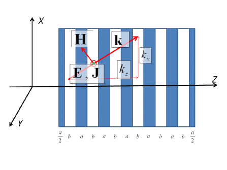
Figure 1: Geometry of wave propagation in the case of s-polarization. Here ${\bf k}=(k_{x},0,k_{z})$ is the wave vector of the external current wave [Eq. (2)]. A finite symmetric slab containing $N=6$ unit cells is shown. Each cell consists of three layers of the widths $(a/2,b,a/2)$. Equivalently, we can view the unit cells as consisting of two layers of the widths $(a,b)$, provided that one half of the first $a$-type layer has been cut off and moved from the left face of the slab to its right face. Note that the sample shown in the figure has a center of symmetry.

We will consider only the special case of s-polarization, when the wave vector ${\bf k}$ lies in the plane $XZ$ of the rectangular frame shown in Fig. 1 and the amplitude ${\bf J}$ of the external current (2) is collinear with the $Y$-axis, so that ${\bf k}=(k_{x},0,k_{z})$ and ${\bf J}=(0,J_{y},0)$. According to (14), this is sufficient to uniquely define the following elements of the effective permittivity and permeability tensors: $\epsilon_{xx}=\epsilon_{yy}$, $\mu_{xx}=\mu_{yy}$ and $\mu_{zz}$.

We will need to introduce the following notations:

$$k_{a}^{2}=k_{0}^{2}\epsilon_{a}\ ,\ \ k_{b}^{2}=k_{0}^{2}\epsilon_{b}\ ,$$ (15a)

$$\kappa_{a}=\sqrt{k_{a}^{2}-k_{x}^{2}}\ ,\ \ \kappa_{b}=\sqrt{k_{b}^{2}-k_{x}^{2}}\ ,$$ (15b)

$$\phi_{a}=\kappa_{a}a\ ,\ \ \phi_{b}=\kappa_{b}b\ ,$$ (15c)

$$\theta_{a}=k_{z}a\ ,\ \ \theta_{b}=k_{z}b\ ,$$ (15d)

$$p_{a}=a/h\ ,\ \ p_{b}=b/h\ ,$$ (15e)

and also the standard homogenization result for a periodic layered medium:

$$\epsilon_{\parallel}=p_{a}\epsilon_{a}+p_{b}\epsilon_{b}\ ,\ \ \epsilon_{\perp}=\frac{1}{p_{a}/\epsilon_{a}+p_{b}/\epsilon_{b}}\ ,$$ (16a)

$$\mu_{\parallel}=\mu_{\perp}=1\ .$$ (16b)

Here the quantities indexed by “$\parallel$” and “$\perp$” give the standard homogenization results for the elements of the permittivity and permeability tensors that correspond to the direction of the electric field parallel and perpendicular to the layers, respectively. Throughout the paper, the branches of all square roots are defined by the condition $0\leq{\rm arg}(\sqrt{z})<\pi$.

We wish to solve Eq. (3) in which $\tilde{\epsilon}({\bf r})$ is equal to $\epsilon_{a}$ in the $a$-type layers and to $\epsilon_{b}$ in the $b$-type layers. Without loss of generality, we can consider the unit cell $0<z\leq h=a+b$, which contains two layers: the first layer ($a$-type) is contained between the planes $z=0$ and $z=a$ and the second ($b$-type) layer is contained between the planes $z=a$ and $z=h$. We can seek the solution in each homogeneous region excluding its boundaries as a particular solution to the inhomogeneous equation plus the general solution to the homogeneous equation, viz,

$$E_{y}(x,z)=e^{i{\bf k}\cdot{\bf r}}\left[{\mathscr{E}}_{p}(z)\hskip 4.2679pt+{\mathscr{E}}_{g}(z)\hskip 4.2679pt\right]\ ,$$ (17a)

$$H_{x}(x,z)=e^{i{\bf k}\cdot{\bf r}}\left[{\mathscr{H}}_{p}(z)+{\mathscr{H}}_{g}(z)\right]\ .$$ (17b)

Here the subscripts “$p$” and “$g$” denote the particular and the general solution, respectively, and the overall exponential factor $\exp(i{\bf k}\cdot{\bf r})$ is written out explicitly.

The particular solution is given by

$${\mathscr{E}}_{p}(z)=J_{y}f(z)\ ,\ \ {\mathscr{H}}_{p}(z)=-\frac{k_{z}}{k_{0}}J_{y}f(z)\ ,$$ (18)

where

$$f(z)=\left\{\begin{array}[]{ll}{\displaystyle\frac{k_{0}^{2}}{k^{2}-k_{a}^{2}}}\equiv f_{a}\ ,&0<z<a\\ {\displaystyle\frac{k_{0}^{2}}{k^{2}-k_{b}^{2}}}\equiv f_{b}\ ,&a<z<h\end{array}\right.\ .\\$$

We emphasize that (18) is a particular solution in the open intervals $0<z<a$ and $a<z<h$. To satisfy boundary conditions at the interfaces, we must add to (18) the general solution to the corresponding homogeneous problem. The latter can be easily stated:

$${\mathscr{E}}_{g}(z)=\hskip 25.60747ptJ_{y}\Delta e^{-ik_{z}z}F_{\mathscr{E}}(z)\ ,$$ (19a)

$${\mathscr{H}}_{g}(z)=-\frac{k_{z}}{k_{0}}J_{y}\Delta e^{-ik_{z}z}F_{\mathscr{H}}(z)\ ,$$ (19b)

where

$$\Delta=f_{b}-f_{a}=\frac{k_{0}^{2}}{k^{2}-k_{b}^{2}}-\frac{k_{0}^{2}}{k^{2}-k_{a}^{2}}$$

and

$$F_{\mathscr{E}}(z)=$$ (20a)

$$\left\{\begin{array}[]{ll}\hskip 25.60747ptA_{a}e^{i\kappa_{a}z}\hskip 17.07164pt+B_{a}e^{-i\kappa_{a}z}\hskip 19.91692pt,&0<z<a\\ e^{i\theta_{a}}[-A_{b}e^{i\kappa_{b}(z-a)}-B_{b}e^{-i\kappa_{b}(z-a)}]\ ,&a<z<h\end{array}\right.\ ;$$ (20d)

$$F_{\mathscr{H}}(z)=$$ (20e)

$$\left\{\begin{array}[]{ll}\hskip 15.649pt{\displaystyle\frac{\kappa_{a}}{k_{z}}}[\hskip 7.11317ptA_{a}e^{i\kappa_{a}z}\hskip 15.649pt-B_{a}e^{-i\kappa_{a}z}\hskip 15.649pt]\ ,&0<z<a\\ {\displaystyle\frac{\kappa_{b}}{k_{z}}}e^{i\theta_{a}}[-A_{b}e^{i\kappa_{b}(z-a)}+B_{b}e^{-i\kappa_{b}(z-a)}]\ ,&a<z<h\end{array}\right.\ .$$ (20h)

In these expressions, various $z$-independent factors have been introduced for convenience and $A_{a},B_{a},A_{b},B_{b}$ is a set of coefficients to be determined from the boundary conditions. The latter require continuity of all tangential field components at the interfaces $z=0,a,h$ and can be stated as follows:

$$F_{\mathscr{E}}(a-0)-F_{\mathscr{E}}(a+0)=e^{i\theta_{a}}\ ,$$ (21a)

$$F_{\mathscr{H}}(a-0)-F_{\mathscr{H}}(a+0)=e^{i\theta_{a}}\ ,$$ (21b)

$$e^{i\theta_{a}}F_{\mathscr{E}}(0)-e^{-i\theta_{b}}F_{\mathscr{E}}(h)=e^{i\theta_{a}}\ ,$$ (21c)

$$e^{i\theta_{a}}F_{\mathscr{H}}(0)-e^{-i\theta_{b}}F_{\mathscr{H}}(h)=e^{i\theta_{a}}\ .$$ (21d)

This results in a set of four equations for the unknown coefficients $A_{a},B_{a},A_{b},B_{b}$, which are stated in Appendix A.

It may seem confusing that the right-hand side in (21) does not go to zero when $J_{y}\rightarrow 0$; in fact, (21) does not contain $J_{y}$ at all. However, the electromagnetic fields $E_{x}(x,z)$ and $H_{y}(x,z)$ computed according to (17)-(19) are proportional to $J_{y}$. Note that the most general solution to (3) is a superposition of the solution derived here (whose amplitude is proportional to $J_{y}$) and the natural Bloch mode of the medium with an arbitrary amplitude. To remove the nonuniqueness, one can either consider the boundary of the medium and thus abandon the infinite medium model, or, alternatively, apply the additional boundary condition requiring “forced” Bloch-periodicity (4). The latter approach is used in current-driven homogenization and in the derivations of this section.

The solution to (21) is given by

$$A_{a}=\frac{{\mathscr{A}}_{a}}{2\mathscr{D}}\ ,\ \ B_{a}=\frac{{\mathscr{B}}_{a}}{2\mathscr{D}}\ ,\ \ A_{b}=\frac{{\mathscr{A}}_{b}}{2\mathscr{D}}\ ,\ \ B_{b}=\frac{{\mathscr{B}}_{b}}{2\mathscr{D}}\ ,$$ (22)

where

$${\mathscr{D}}=\cos(k_{z}h)-\cos(q_{z}h)$$ (23)

and the closed-form expressions for ${\mathscr{A}}_{a}$, ${\mathscr{B}}_{a}$, ${\mathscr{A}}_{b}$ and ${\mathscr{B}}_{b}$ are given in Appendix A. In (23), $q_{z}$ is the $z$-projection of the natural Bloch wave vector ${\bf q}$ computed under the assumption that its $X$-projection is equal to $k_{x}$ (that is, $q_{x}=k_{x}$). The factor $\cos(q_{z}h)$ is defined by the equation

$$\cos(q_{z}h) =\cos(\phi_{a})\cos(\phi_{b})$$ (24)

$$-\frac{1}{2}\left(\frac{\kappa_{a}}{\kappa_{b}}+\frac{\kappa_{b}}{\kappa_{a}}\right)\sin(\phi_{a})\sin(\phi_{b})\ .$$

Evidently, if $k_{z}=\pm q_{z}+2\pi n/h$, where $n$ is an arbitrary integer, the matrix in (21) is singular.

We now simplify the expression for the electric field $E_{y}(x,z)$. After some rearrangement, we can write

$$E_{y}(x,z)=\hskip 142.26378pt$$

$$\frac{J_{y}k_{0}^{4}e^{i{\bf k}\cdot{\bf r}}}{(k^{2}-k_{a}^{2})(k^{2}-k_{b}^{2})}\frac{1}{\mathscr{D}}\left\{\begin{array}[]{ll}F_{a}(z),&0<z<a\\ F_{b}(z),&a<z<h\end{array}\right.\ ,$$

where

$$F_{a}(z)={\mathscr{D}} \frac{k^{2}-k_{b}^{2}}{k_{0}^{2}}+\frac{1}{2}e^{-ik_{z}z}(\epsilon_{b}-\epsilon_{a})$$

$$\times\left[{\mathscr{A}}_{a}e^{i\kappa_{a}z}+{\mathscr{B}}_{a}e^{-i\kappa_{a}z}\right]\ ,$$ (26a)

$$F_{b}(z)={\mathscr{D}} \frac{k^{2}-k_{a}^{2}}{k_{0}^{2}}-\frac{1}{2}e^{ik_{z}(a-z)}(\epsilon_{b}-\epsilon_{a})$$

$$\times\left[{\mathscr{A}}_{b}e^{i\kappa_{b}(z-a)}+{\mathscr{B}}_{b}e^{-i\kappa_{b}(z-a)}\right]\ .$$ (26b)

The $yy$-component of the nonlocal permittivity tensor $\Sigma(\omega,{\bf k})$ is computed by using (8) or (9), which results in

$$\Sigma_{yy}(\omega,{\bf k})=\frac{Q_{a}\epsilon_{a}+Q_{b}\epsilon_{b}}{Q_{a}+Q_{b}}\ ,$$ (27)

where

$$Q_{a}=\int_{0}^{a}F_{a}(z)dz\ ,\ \ Q_{b}=\int_{a}^{h}F_{b}(z)dz\ .$$ (28)

The integrals in (28) are easily computed analytically; these intermediate results are omitted. Note that $Q_{a}$ and $Q_{b}$ depend implicitly on both $\omega$ and ${\bf k}$, which are considered as mathematically-independent variables in the current-driven homogenization theory; this dependence is indicated explicitly in the notation $\Sigma(\omega,{\bf k})$.

Equations (26)-(28) together with the expressions for the expansion coefficients given in Appendix A constitute a closed-form solution for $\Sigma_{yy}(\omega,{\bf k})$. This solution contains only elementary functions, has no branch ambiguities [see the note after Eq. (15)] and can be easily programmed. Note that the quantities $Q_{a}$ and $Q_{b}$ defined in (28) have no singularities when viewed as functions of ${\bf k}$. However, $\Sigma_{yy}(\omega,{\bf k})$ has singularities at the roots of the equation $Q_{a}+Q_{b}=0$. This completes Step One of the current-driven homogenization prescription, at least for the case of s-polarization.

We now proceed with Step Two. For the local effective permittivity, we have

$$\epsilon_{yy}=\Sigma_{yy}(\omega,0)=\left.\frac{Q_{a}\epsilon_{a}+Q_{b}\epsilon_{b}}{Q_{a}+Q_{b}}\right|_{{\bf k}=0}\ .$$

We note that this expression contains the dynamic correction to the permittivity fn (6). From symmetry, we also have $\epsilon_{xx}=\epsilon_{yy}$. The remaining nontrivial component of the permittivity tensor is $\epsilon_{zz}$; this element cannot be computed by considering only s-polarization of the external current.

To compute the elements of the permeability tensor, we use the first equality in (14a) and the second equality in (14c). More specifically, we have

$$\beta_{xx}=\frac{k_{0}^{2}}{2}\left.\frac{\partial^{2}\Sigma_{yy}}{\partial k_{z}^{2}}\right|_{{\bf k}=0}\ ,\ \ \beta_{zz}=\frac{k_{0}^{2}}{2}\left.\frac{\partial^{2}\Sigma_{yy}}{\partial k_{x}^{2}}\right|_{{\bf k}=0}\ .$$

Using (27), we can obtain the following formulas for $\beta_{xx}$ and $\beta_{zz}$ in terms of $Q_{a}$ and $Q_{b}$:

$$\beta_{xx}=\left.k_{0}^{2}(\epsilon_{b}-\epsilon_{a})\frac{Q_{a}Q_{b}^{(zz)}-Q_{b}Q_{a}^{(zz)}}{(Q_{a}+Q_{b})^{2}}\right|_{{\bf k}=0}\ ,$$ (29a)

$$\beta_{zz}=\left.k_{0}^{2}(\epsilon_{b}-\epsilon_{a})\frac{Q_{a}Q_{b}^{(xx)}-Q_{b}Q_{a}^{(xx)}}{(Q_{a}+Q_{b})^{2}}\right|_{{\bf k}=0}\ .$$ (29b)

In these expressions, $Q_{a}^{(xx)}$ denotes the second derivative of $Q_{a}$ with respect to $k_{x}$ evaluated at ${\bf k}=0$, etc. In deriving (29), we have used the fact that $Q_{a}^{(x)}=Q_{a}^{(z)}=Q_{b}^{(x)}=Q_{b}^{(z)}=0$. Note that equation (29) is invariant under the permutation of indexes $a\leftrightarrow b$.

The elements of the effective permeability tensor are expressed in terms of $\beta_{xx}$, $\beta_{zz}$ as

$$\mu_{xx}=\frac{1}{1-\beta_{xx}}\ ,\ \ \mu_{zz}=\frac{1}{1-\beta_{zz}}\ .$$ (30)

From symmetry, we also have $\mu_{yy}=\mu_{xx}$. Closed-form expressions for $\epsilon_{xx}=\epsilon_{yy}$, $\mu_{xx}=\mu_{yy}$ and $\mu_{zz}$ are given in Appendix B. These expressions contain only elementary trigonometric functions but are fairly cumbersome. However, the small-$h$ asymptotic approximations of these expressions have the following simple form:

$$\epsilon_{xx} =\epsilon_{yy}=\epsilon_{\parallel}+\frac{\left(\epsilon_{a}-\epsilon_{b}\right)^{2}}{12}$$

$$\times\left(p_{a}p_{b}\right)^{2}\left(k_{0}h\right)^{2}+O(h^{4})\ ,$$ (31a)

$$\mu_{xx} =\mu_{yy}=1+\frac{\left(\epsilon_{a}-\epsilon_{b}\right)^{2}}{240}$$

$$\times\left(p_{a}p_{b}\right)^{2}(1+2p_{a}p_{b})(k_{0}h)^{4}+O(h^{6})\ ,$$ (31b)

$$\mu_{zz} =1-\frac{\left(\epsilon_{a}-\epsilon_{b}\right)^{2}}{720}$$

$$\times\left(p_{a}p_{b}\right)^{2}(1+2p_{a}p_{b})(k_{0}h)^{4}+O(h^{6})\ .$$ (31c)

Thus, the first nonvanishing corrections to the effective permeability tensor are obtained to fourth order in $h$. Moreover, the corrections to $\mu_{xx}$ and $\mu_{zz}$ differ by the constant factor $-3$. Consequently, current-driven homogenization, when applied to the 1D periodic structure considered in this section, guarantees that at least one of the principal values of the permeability tensor has a negative imaginary part for sufficiently small values of $h$, provided that ${\rm Im}(\epsilon_{a}-\epsilon_{b})^{2}\neq 0$.

IV Transmission and reflection by homogeneous and layered slabs

In what follows, we will need to refer to the formulas for the transmission ($T$) and reflection ($R$) coefficients of homogeneous and layered slabs. These formulas are well known and are adduced here mainly for reference. However, they also reveal some important features that will help us analyze the numerical results of the next section. We still work in the geometry of Fig. 1 and, in analogy to (15b), denote the $z$-projection of the incident wave vector by $\kappa_{0}$, so that

$$\kappa_{0}=\sqrt{k_{0}^{2}-k_{x}^{2}}\ .$$

Note that, for $k_{x}>k_{0}$, the incident wave is evanescent. All formulas given below are parameterized by $k_{x}$.

Any slab with a one-dimensional distribution of electromagnetic parameters is completely characterized by its characteristic matrix $M$. Suppose the slab occupies the region $0<z<L$. Then the tangential components of the electric and magnetic field at the left and right faces of the slab are related by

$$\begin{bmatrix}E_{L}\\ H_{L}\end{bmatrix}=\begin{bmatrix}M_{11}&M_{12}\\ M_{21}&M_{22}\\ \end{bmatrix}\begin{bmatrix}E_{0}\\ H_{0}\end{bmatrix}\ .$$

The general property of all characteristic matrices is ${\rm det}(M)=1$. If the slab has a center of symmetry (as is the case in this paper), the left and right incidence directions are equivalent which can be mathematically stated as $M_{11}=M_{22}$. Under these conditions, the transfer matrix can be written as Feng (2010)

$$M=\begin{bmatrix}\hskip 19.91692pt\cos\theta&(-i/{\mathscr{Z}})\sin\theta\\ -i{\mathscr{Z}}\sin\theta&\hskip 34.1433pt\cos\theta\\ \end{bmatrix}\ ,$$

where $\theta$ and ${\mathscr{Z}}$ are the optical depth and the generalized impedance of the slab fn (2).

The transmission and reflection coefficients can be expressed in terms of $\theta$ and ${\mathscr{Z}}$ as

$$T=\frac{1}{\cos\theta-iX_{+}\left({\mathscr{Z}}_{0},{\mathscr{Z}}\right)\sin\theta}\ ,$$ (32a)

$$R=\frac{-iX_{-}\left({\mathscr{Z}}_{0},{\mathscr{Z}}\right)\sin\theta}{\cos\theta-iX_{+}\left({\mathscr{Z}}_{0},{\mathscr{Z}}\right)\sin\theta}\ ,$$ (32b)

where

$$X_{\pm}({\mathscr{Z}}_{1},{\mathscr{Z}}_{2})=\frac{1}{2}\left(\frac{{\mathscr{Z}}_{1}}{{\mathscr{Z}}_{2}}\pm\frac{{\mathscr{Z}}_{2}}{{\mathscr{Z}}_{1}}\right)$$

and ${\mathscr{Z}}_{0}=\kappa_{0}/k_{0}$ is the generalized impedance of free space (we assume that the slab is embedded in a vacuum or air). The quantities $T$ and $R$ defined in (32) relate the amplitudes of the transmitted and reflected tangential field (electric in the case of s-polarization or magnetic field in the case of p-polarization) measured at the planes $z=L$ (for $T$) or $z=0$ (for $R$) to the amplitude of the incident wave at $z=0$. The specific expressions for $\theta$ and ${\mathscr{Z}}$ depend on polarization and it should be kept in mind that, at normal incidence, $T_{s}=T_{p}$ but $R_{s}=-R_{p}$, where the subscripts indicate the particular mathematical expression applicable to a given polarization state.

Specific expressions for $\theta$ and ${\mathscr{Z}}$ for homogeneous and layered slabs are given below.

Homogeneous Anisotropic Slab.

Consider a slab characterized by purely local diagonal tensors $\epsilon={\rm diag}(\epsilon_{\perp},\epsilon_{\perp},\epsilon_{\parallel})$ and $\mu={\rm diag}(\mu_{\perp},\mu_{\perp},\mu_{\parallel})$. Then

$$\theta=q_{z}L\ ,\ \ {\mathscr{Z}}=q_{z}/(k_{0}\eta_{\parallel})\ ,$$ (33)

where

$$q_{z}=\sqrt{k_{0}^{2}\epsilon_{\parallel}\mu_{\parallel}-k_{x}^{2}\left(\eta_{\parallel}/\eta_{\perp}\right)}$$ (34)

and $\eta$ refers to $\mu$ for s-polarization and to $\epsilon$ for p-polarization.

Layered Slab.

Consider a layered slab of total width $L=Nh$ containing $N$ unit cells arranged as shown in Fig. 1. Each cell consists of three consecutive layers of the widths $(a/2,b,a/2)$, where $a+b=h$, and the permittivities $\epsilon_{a}$ and $\epsilon_{b}$, respectively. Then

$$\theta=q_{z}L=Nq_{z}h\ ,$$ (35a)

$${\mathscr{Z}^{2}}={\mathscr{Z}}_{a}^{2}$$

$$\times\frac{\sin\phi_{a}\cos\phi_{b}-X_{-}\sin\phi_{b}+X_{+}\cos\phi_{a}\cos\phi_{b}}{\sin\phi_{a}\cos\phi_{b}+X_{-}\sin\phi_{b}+X_{+}\cos\phi_{a}\cos\phi_{b}}\ .$$ (35b)

Here $\phi_{a},\phi_{b}$ are defined in (15c), $X_{\pm}=X_{\pm}({\mathscr{Z}}_{a},{\mathscr{Z}}_{b})$, ${\mathscr{Z}}_{a}$ and ${\mathscr{Z}}_{b}$ are the generalized impedances of each layer and $q_{z}$ is the natural Bloch wave number of the medium defined by the following equation:

$$\cos(q_{z}h)=\cos(\phi_{a})\cos(\phi_{b})-X_{+}\sin(\phi_{a})\sin(\phi_{b})\ .$$ (36)

Note that (24) is a special case of (36) (for s-polarization and nonmagnetic layers). Also Eq. (36) defines $\cos(q_{z}h)$ but not $\sin(q_{z}h)$. The latter quantity can be computed by using one of the formulas

$$\sin(q_{z}h)$$

$$=\frac{\mathscr{Z}}{{\mathscr{Z}}_{a}}\left(\sin\phi_{a}\cos\phi_{b}+X_{-}\sin\phi_{b}+X_{+}\cos\phi_{a}\sin\phi_{b}\right)$$

$$=\frac{{\mathscr{Z}}_{a}}{\mathscr{Z}}\left(\sin\phi_{a}\cos\phi_{b}-X_{-}\sin\phi_{b}+X_{+}\cos\phi_{a}\sin\phi_{b}\right)\ ,$$

where ${\mathscr{Z}}$ is determined by taking an arbitrary branch of the square root of (35); the resultant transfer matrix is invariant with respect to this choice.

The formulas given above illustrate several important points. First, the transmission of a thick, highly transparent slab is very sensitive to small errors in $q_{z}$. This is because the trigonometric functions such as $\cos\theta=\cos(q_{z}L)$ incur a substantial phase shift when $q_{z}$ is changed by $\sim\pi/L$. If $L\rightarrow\infty$ (and losses can still be ignored), any homogenization theory is expected to be unstable numerically because a small error in medium parameters can propagate to become a significant error in $T$. This instability, however, is of little practical importance because, in most cases, the illumination is not monochromatic. What we are discussing here are, essentially, the resonances of a Fabry-Perot etalon. In most applications to optical imaging and microscopy, illumination is more broadband than a line of a single-mode laser and the interference effects are unobservable. Under these conditions, the expressions (32) can be regularized by Gaussian integration with respect to $k_{0}$ or $L$. However, in this paper, we only consider strictly monochromatic light.

Second, an error in the generalized impedance will also result in an error in both $T$ and $R$ and, in some cases, this error can also be dramatic. An illustrative example is the case $X_{+}\rightarrow-1$, which is the operation regime of the so-called perfect lens Pendry (2000). Indeed, we can re-write (32a) as

$$T=\frac{2}{(1-X_{+})\exp(i\theta)+(1+X_{+})\exp(-i\theta)}\ .$$ (37)

If $X_{+}$ is exactly equal to $-1$, (37) predicts $T=\exp(-i\theta)$. For evanescent waves and a macroscopically-thick slab, the factor $\exp(i\theta)$ is exponentially small. Therefore, if we make a small error fn (5) in $X_{+}$, say, $X_{+}=-1+\delta$, such that $|\exp(i\theta)|\ll|\delta|\ll 1$, Eq. (37) would predict $T=(2/\delta)\exp(i\theta)$, which is dramatically different from the former result. We note that there are other similar situations and that the condition $X_{+}\approx-1$ is not special in this respect.

Therefore, a homogenization theory must predict correctly both the optical depth and the impedance of a medium. But can local effective medium parameters be found in such a way as to predict $\theta$ and ${\mathscr{Z}}$ correctly and simultaneously? Standard EMTs do allow this asymptotically in the limit $h\rightarrow 0$. In contrast, extended EMTs that consider an infinite medium cannot predict correctly the impedance of the medium. The current-driven homogenization theory is of this variety: it predicts correctly the first nonvanishing correction to $\theta$ (compared to the standard homogenization result) but does not provide any meaningful corrections or approximations to ${\mathscr{Z}}$. Moreover, this correction to $\theta$ yields a valid approximation only in a limited range of $h$, as will be shown below. In a more general case, it is not possible to find local parameters that predict correctly (for all angles of incidence) even $\theta$ alone. Therefore, the claims that the current-driven homogenization theory is rigorous and completely general Silveirinha (2007, 2009); Alu (2011) are exaggerated.

We finally note that the above analysis could be extended to three-dimensional orthorhombic lattices by integrating out higher-order harmonics in the $xy$-plane, i.e. by low-pass filtering.

V Numerical examples

In this section, we consider several examples of computing the local effective parameters of one-dimensional layered media according to the current-driven homogenization prescription. We note that the maximum possible value of the numerical factor $\left(p_{a}p_{b}\right)^{2}(1+2p_{a}p_{b})$ in (31) is $3/32$ and it is achieved when $p_{a}=p_{b}=1/2$. These volume fractions are used in all the numerical examples shown below. The $b$-type medium is assumed to be air or vacuum with $\epsilon_{b}=1$. For the $a$-type medium, three different examples will be considered. In Example A, the $a$-type medium is a lossy dielectric considered at a fixed frequency and varying values of $h$ and $k_{x}$. Example B is similar to example A, but the $a$-type medium is a conductor. In Example C, the $a$-type medium is an idealized Drudean metal considered at a fixed value of $h$, $k_{x}=0$ and varying $\lambda_{0}$. Thus, in Example C we account for the frequency dispersion in metal.

The results of current-driven homogenization will be compared to the standard homogenization result (16) and to the results of S-parameter retrieval Koschny et al. (2003); Chen et al. (2004); Feng (2010); Menzel et al. (2008). As is well known, retrieving effective parameters of a slab from the transmission and reflection coefficients at normal or near-normal incidence is an ill-posed inverse problem. We have used several different methods of regularizing the inverse solution, some of which have been proposed in the literature Chen et al. (2004) and others have been devised by us; see Appendix C for full details. All these various modalities of the retrieval technique yield approximately the same result when $h/\lambda_{0}\ll 1$ but deviate strongly for larger values of this ratio. In the figures below, the retrieval results are shown only for the range of $h/\lambda_{0}$ within which the technique is numerically stable.

V.1 Example A

We start with the case where the $a$-type medium is a lossy dielectric characterized by $\epsilon_{a}=4.0+0.1i$ at a given wavelength $\lambda_{0}$. In Example A, we assume that $h$ and $k_{x}$ can vary while $\lambda_{0}$ is fixed. Then the physically-measurable quantities of interest are functions of the dimensionless variables $h/\lambda_{0}$ and $k_{x}/k_{0}$, and the actual value of $\lambda_{0}$ is unimportant. The sample consists of $N=50$ symmetric unit cells of the type $(a/2,b,a/2)$ arranged as shown in Fig. 1. As noted above, we take $a=b=h/2$ in all numerical experiments.

In Figs. 2-4, we illustrate the predictions of current-driven homogenization for all the components of the permittivity and permeability tensors that can be obtained in s-polarization. The results are compared to the predictions of the S-parameter retrieval method. It can be seen that current-driven homogenization produces the standard homogenization result when $h\rightarrow 0$. This much could be inferred from considering the asymptotic expansions (31). In fact, for $h/\lambda_{0}\lesssim 0.2$, all curves displayed in the figures are close to the standard homogenization result. We note that this is, approximately, the same range of $h$ in which S-parameter retrieval is numerically stable. The interpretation of this fact is obvious: for sufficiently small ratios of $h/\lambda_{0}$, the transmission and reflection properties of the sample are well fitted by purely local effective permittivity $\epsilon$ and $\mu=1$.

Both current-driven homogenization and S-parameter retrieval provide corrections to the standard homogenization result. As long as these corrections are small, they can yield a homogenization result that appears to be “reasonable”. Yet, all the dramatic features of current-driven homogenization occur for $h/\lambda_{0}>0.2$, where the S-parameter retrieval is unstable (that is, the retrieved result strongly depends on the particular implementation of the retrieval technique). In particular, the resonance in $\mu_{xx}$ occurs at $h/\lambda_{0}\approx 0.4$. Is this result physically reasonable? We will address this question now by considering the transmission and reflection coefficients of a finite slab.

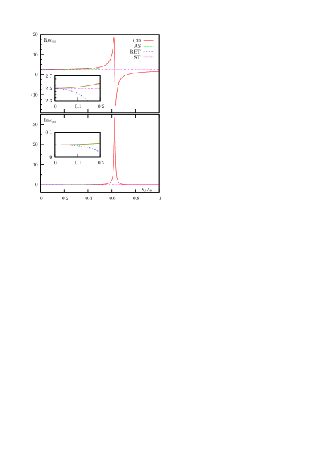
Figure 2: Example A. Real (top) and imaginary (bottom) parts of $\epsilon_{yy}$ as functions of $h/\lambda_{0}$. The various curves shown are obtained as follows: CD - by current-driven homogenization [formulas given in Appendix B]; AS - the small-$h$ asymptotes of the former [Eq. (31)]; RET - by S-parameter retrieval [see Appendix C]; and ST - the standard homogenization result $\epsilon_{\parallel}$ [defined in Eq. (16a)]. Insets show the details of all curves for small $h$.

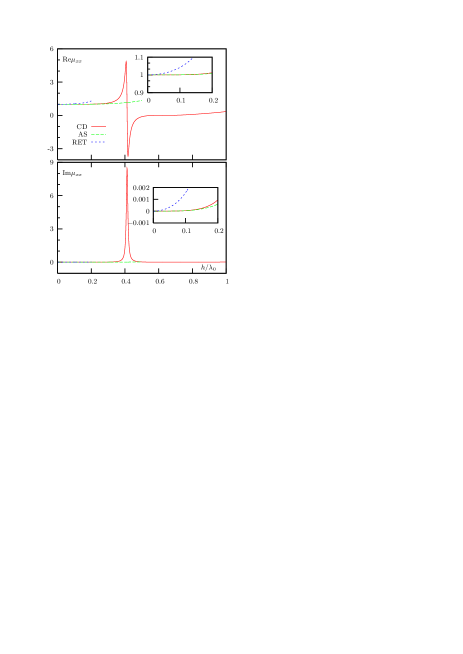
Figure 3: Example A. Same as in Fig. 2 but for $\mu_{xx}$. The standard homogenization result $\mu_{xx}=1$ is not shown.

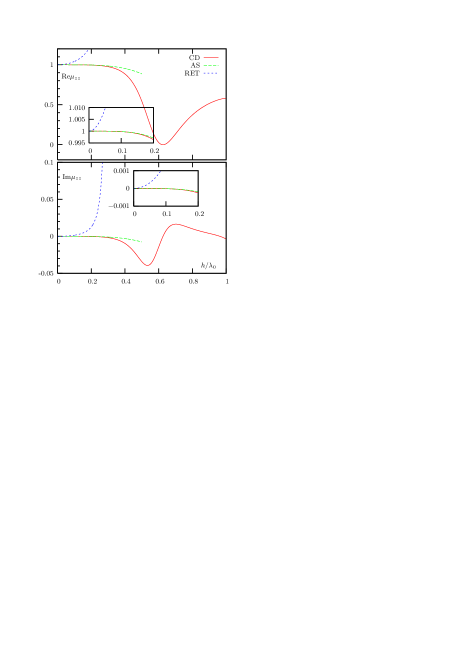
Figure 4: Example A. Same as in Fig. 2 but for $\mu_{zz}$. The standard homogenization result $\mu_{zz}=1$ is not shown.

In Fig. 5, we plot $|T|^{2}$ and $|R|^{2}$ at normal incidence as functions of $h/\lambda_{0}$. It can be seen that the different methods used to compute the transmittance and reflectance yield very similar result for $h/\lambda_{0}\lesssim 0.2$ but very different results for $h/\lambda_{0}>0.2$. Overall, when both $T$ and $R$ are considered, current-driven homogenization does not provide a meaningful correction to the standard homogenization result (16). In other words, at small $h/\lambda_{0}$, both methods predict approximately the same result while at larger values of $h/\lambda_{0}$ both methods simultaneously fail. This is clearly visible in the case of $R$ but is also true for $T$, which is very small when $h/\lambda_{0}>0.4$. In the latter case, both current-driven and standard homogenization generate relative errors in $|T|^{2}$ of many orders of magnitude, as could be verified by utilizing logarithmic vertical scale (data not shown). Of course, this result is expected for standard homogenization, which is an asymptotic theory. However, the current-driven homogenization theory was claimed to have predictive power beyond the limit of small $h$ and, in particular, in the region of the parameter space where it predicts nontrivial magnetic effects. This claim appears not to be supported by the data of Fig. 5.

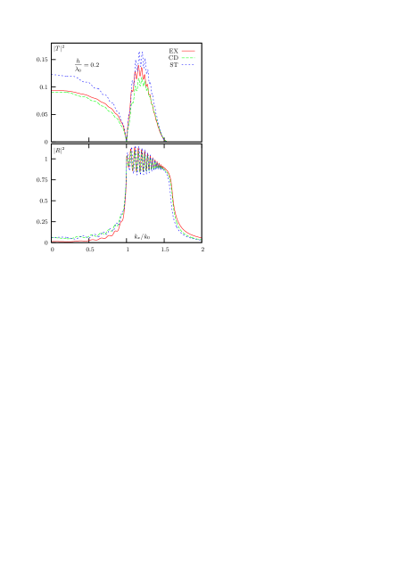
Figure 6: Example A. Absolute values squared of the transmission (top) and reflection (bottom) coefficients computed as functions of $k_{x}/k_{0}$ for $h/\lambda_{0}=0.2$. Same curve labels as in Fig. 5 have been used.

Nevertheless, if we focus on $T$ alone, current-driven homogenization provides a slightly more accurate result compared to standard homogenization when $h/\lambda_{0}$ is in a small vicinity of $0.2$. Let us, therefore, consider in more detail transmission and reflection by the slab at $h/\lambda_{0}=0.2$. The effective parameters obtained at this value of $h/\lambda_{0}$ by current-driven homogenization are listed in Table 1 and the dependence of $|T|^{2}$ and $|R|^{2}$ on the angle of incidence is illustrated in Fig. 6. In the case of $T$, current-driven homogenization provides a noticeable improvement over the standard homogenization result when $k_{x}<k_{0}$ (in fact, the standard formula predicts the phase of $T$ incorrectly in this range of $k_{x}$) but not when $k_{x}>k_{0}$, i.e., not when the incident wave is evanescent. In the case of $|R|^{2}$, no improvement is observed. We note that the values of $|R|^{2}$ in Fig. 6 can exceed unity for $k_{x}>k_{0}$, when both the incident and the reflected waves are evanescent.

We will discuss below the reason why current-driven homogenization predicts $|T|^{2}$ more accurately than the standard homogenization result at $h/\lambda_{0}=0.2$, but it is useful to note right away that this has nothing to do with an accurate prediction of $\mu$. In fact, the values of $\mu$ computed by current-driven homogenization are not optimal. To illustrate this point, consider the data of Fig. 7. Here we plot the real parts of $T$ and $R$ and introduce two additional curves. The first of these curves (labeled CD-REN) was obtained by taking the current-driven effective parameters listed in Table 1 and renormalizing them according to the formula

$$\epsilon\rightarrow\xi\epsilon\ ,\ \ \mu\rightarrow\mu/\xi\ .$$ (38)

with the renormalization factor $\xi=\mu_{xx}$. In (38), $\epsilon$ nd $\mu$ are tensors while $\xi$ is a scalar. Renormalization (38) does not affect the equivalence of the induced currents (10) and (12) when each formula is evaluated on-shell, that is, for ${\bf k}={\bf q}$. The renormalized parameters are also given in Table 1. It can be seen that the renormalized effective parameters have dramatically different values of $\mu-1$. Yet, $T$ and $R$ computed by using both sets of parameters are virtually indistinguishable.

Moreover, the effective parameters obtained by current-driven homogenization are in no way optimal if the goal of homogenization is to fit the transmission and reflection data as closely as possible. The latter aim is, in fact, achieved by the S-parameter retrieval procedure. In Fig. 7 we show an additional curve (labeled RET), which was computed using the effective parameters obtained by S-parameter retrieval. More specifically, $\epsilon_{yy}$ and $\mu_{xx}$ have been computed by Method 2 and $\mu_{zz}$ was computed by Method 3, where the various methods of S-parameter retrieval are described in Appendix C. The particular choice of methods is explained as follows: Method 2 is more stable numerically but, unlike Method 3, it does not allow one to compute $\mu_{zz}$. Returning to Fig. 7, we observe that the curve labeled RET provides a much better fit to both $T$ and $R$ in a wide range of incidence angles. This is in spite of the fact that the effective parameters labeled as RET in Table 1 are very different from those labeled as either CD or CD-REN.

At this point, we note that the magnetic effects predicted by current-driven homogenization at $h/\lambda_{0}=0.2$ are tiny; $|\mu-1|$ does not exceed $\sim 0.01$ and the condition of weak nonlocality is very well satisfied. Yet the relative errors in $T$ and $R$ produced by current-driven homogenization are significant – they are at least of the same order of magnitude as $|\mu-1|$ or greater. In particular, the relative errors in ${\rm Re}(R)$ or $|R|^{2}$ at normal incidence exceed $100\%$. To distinguish the two effects, it would suffice to measure the reflection coefficient at normal incidence.

Effective
Parameters	$h/\lambda_{0}=0.2$	$h/\lambda_{0}=0.3$
	ST
$\epsilon_{\parallel}$	$2.50+i0.05$
$\mu_{\parallel}$	$1+i0$
$\mu_{\perp}$	$1+i0$
	CD
$\epsilon_{yy}-\epsilon_{\parallel}$	$(820.+i56.6)10^{-4}$	$(21.4+i6.05)10^{-2}$
$\mu_{xx}-1$	$(126.+i9.45)10^{-4}$	$(11.5+i1.11)10^{-2}$
$\mu_{zz}-1$	$-(35.9+i2.55)10^{-4}$	$-(24.0+i1.84)10^{-3}$
$n=\epsilon_{yy}\mu_{xx}$	$(261.+i5.88)10^{-2}$	$(30.3+i1.03)10^{-1}$
	CD-REN
$\epsilon_{yy}-\epsilon_{\parallel}$	$(114.+i8.80)10^{-3}$	$(52.5+i5.32)10^{-2}$
$\mu_{xx}-1$	$0$	0
$\mu_{zz}-1$	$-(16.0+i1.17)10^{-3}$	$-(12.5+i1.04)10^{-2}$
$n=\epsilon_{yy}\mu_{xx}$	$(261.+i5.88)10^{-2}$	$(30.3+i1.03)10^{-1}$
	RET
$\epsilon_{yy}-\epsilon_{\parallel}$	$-(48.4+i3.07)10^{-2}$	N/A
$\mu_{xx}-1$	$(30.3+i1.74)10^{-2}$	N/A
$\mu_{zz}-1$	$(25.9+i1.27)10^{-2}$	N/A
$n=\epsilon_{yy}\mu_{xx}$	$(263.+i6.03)10^{-2}$	N/A

Table 1: Effective parameters for Example A obtained by various methods at $h/\lambda_{0}=0.2$ and $h/\lambda_{0}=0.3$. ST - the standard homogenization result; CD - current-driven homogenization; CD-REN - current-driven homogenization with renormalization (38); RET - retrieved parameters. The numbers have been rounded off to three significant figures. However, all plots shown in this paper utilize either double or quadruple-precision computations.

Now let us turn to the case $h/\lambda_{0}=0.3$, which is illustrated in Figs. 8,9. S-parameter retrieval is unstable at this point and standard homogenization is inapplicable (the corresponding curves are not shown). Therefore, if current-driven homogenization could produce reasonable predictions at $h/\lambda_{0}=0.3$, it would constitute a valid and useful approximation. However, the data of Figs. 8,9 do not support this hypothesis. The relative errors in $R$ and $T$ for current-driven homogenization are at this point dramatic and can be many orders of magnitude. For $k_{x}<k_{0}$, the relative errors are many orders of magnitude in $T$ and at least an order of magnitude in $R$. Both the phase and the amplitude of $T$ and $R$ are predicted with significant errors in the whole range of $k_{x}$ considered. We note that, in the bottom plot of Fig. 9, the real part of $R$ is reproduced correctly at normal incidence by current-driven homogenization. However, as can be seen from the data of Fig. 8, $|R|^{2}$ at normal incidence is predicted with a large error. Consequently, ${\rm Im}R$ is also predicted with a large error (data not shown).

All this is in spite of the fact that current-driven homogenization does not yet predict any dramatic magnetic effects at $h/\lambda_{0}=0.3$. Indeed, for this value of $h/\lambda_{0}$, current-driven homogenization predicts that $|\mu-1|$ does not exceed $\approx 0.1$. Moreover, in can be seen from the data of Figs. 8,9 that renormalization of effective parameters according to (38) does not worsen or, indeed, noticeably modify the predictions of current-driven homogenization.

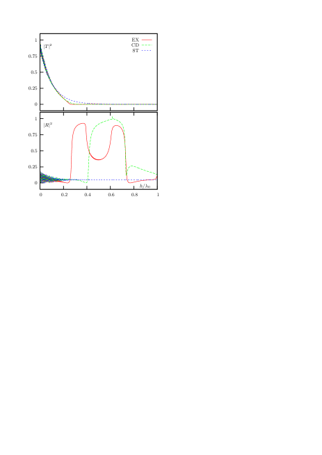
Figure 5: Example A. Absolute values squared of the transmission (top) and reflection (bottom) coefficients at normal incidence as functions of $h/\lambda_{0}$. The various curves shown are obtained as follows: EX - the exact result [Eqs. (32)]; CD - equivalent homogeneous slab with current-driven effective parameters; and ST - same as above but for effective parameters obtained by standard homogenization.

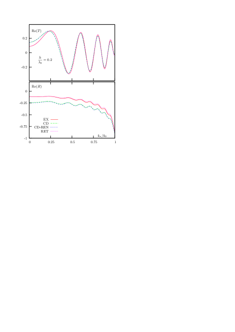
Figure 7: Example A. Same as in Fig. 6 but for the real parts of $T$ and $R$. Additional curve labels: CD-REN - current-driven homogenization with renormalization (38); and RET - S-parameter retrieval. See Table 1 for numerical values of the effective parameters used for each curve. Note that CD and CD-REN curves are visually indistinguishable; EX and RET curves are indistinguishable in the upper plot but slightly different in the bottom plot.

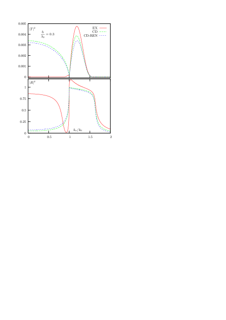
Figure 8: Example A. Same as in Fig. 6 but for $h/\lambda_{0}=0.3$.

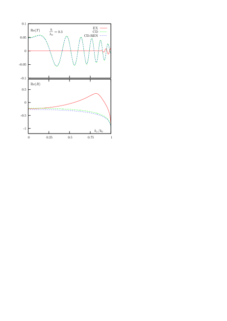
Figure 9: Example A. Same as in Fig. 7 but for $h/\lambda_{0}=0.3$.

At even larger values of $h/\lambda_{0}$, predictions of current-driven homogenization are widely inaccurate. In particular, current-driven homogenization cannot be relied upon at $h/\lambda_{0}=0.4$, when $\mu_{xx}$ experiences a dramatic resonance. This is evident from the data of Fig. 5 and there is no need to support this conclusion with additional graphics. A question, however, remains: why did we observe a moderate improvement in $T$ at $h/\lambda_{0}=0.2$? The reason is that current-driven homogenization provides a first nonvanishing correction to the Bloch wave number $q_{z}$ but not to the impedance ${\mathscr{Z}}$. Both quantities enter the formulas for $T$ and $R$ (32). As was discussed in Sec. IV, under some circumstances, $T$ can be more sensitive to errors in $q_{z}$ than to errors in ${\mathscr{Z}}$. This does not mean that errors in ${\mathscr{Z}}$ are insignificant. As could be seen in Figs. 7, an error in the impedance that current-driven homogenization entails translates into an error in $T$ and $R$, which is at least of the same order of magnitude or greater than $|\mu-1|$.

The above point is illustrated in Figs. 10,11. Here we plot $q_{z}h$ and ${\mathscr{Z}}$ at normal incidence as functions of $h/\lambda_{0}$; predictions of current-driven and standard homogenization are compared to the exact result given in (35),(36). It can be seen that, at $h/\lambda_{0}\approx 0.2$, current-driven homogenization provides a slightly more accurate result for $q_{z}$. In the case of ${\mathscr{Z}}$, current-driven homogenization does not provides a better approximation at any value of $h/\lambda_{0}$.

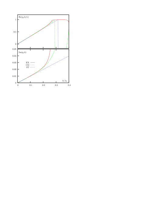
Figure 10: Example A. Real (top) and imaginary (bottom) parts of the unit cell optical depth parameter, $q_{z}h$, at normal incidence as a function of $h/\lambda_{0}$.

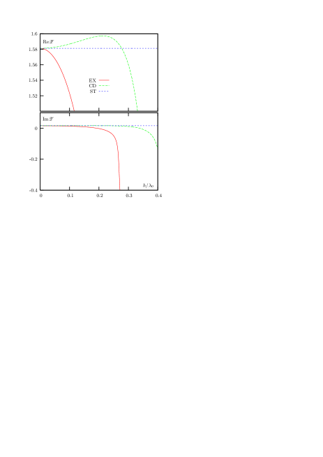
Figure 11: Example A. Real (top) and imaginary (bottom) parts of the generalized impedance ${\mathscr{Z}}$, at normal incidence as a function of $h/\lambda_{0}$.

V.2 Example B

We now turn to the case when the $a$-type medium is a high-conductivity metal with $\epsilon_{a}=-3+0.01i$ at a given fixed wavelenghth $\lambda_{0}$. The sample consists of $5$ symmetric unit cells of the type $(a/2,b,a/2)$, where $a=b$ as before. Effective parameters for Example B are plotted as functions of $h/\lambda_{0}$ in Figs. 12-14. Current-driven homogenization predicts that $\mu_{xx}$ experiences a resonance near the point $h/\lambda_{0}=0.75$ while $\mu_{zz}$ exhibits no dramatic effects.

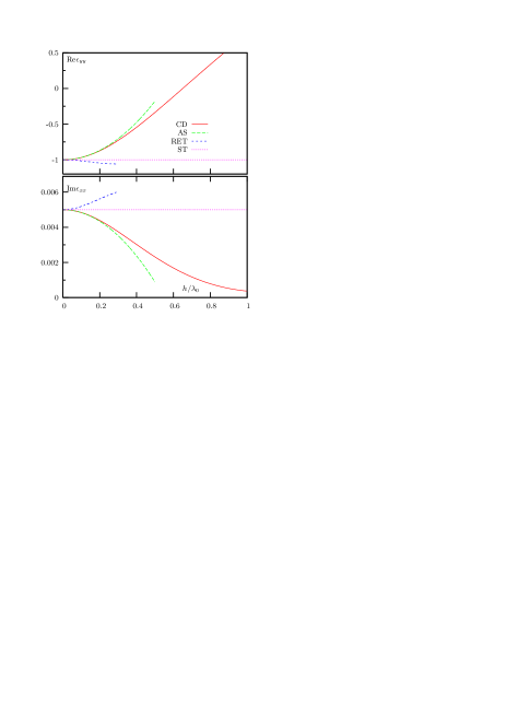
Figure 12: Example B. Real (top) and imaginary (bottom) parts of $\epsilon_{yy}$ as functions of $h/\lambda_{0}$. Same curve labels as in Fig. 2 have been used.

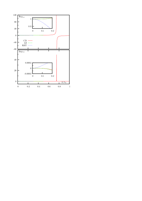
Figure 13: Example B. Same as in Fig. 12 but for $\mu_{xx}$. The standard homogenization result $\mu_{xx}=1$ is not shown.

Figure 14: Example B. Same as in Fig. 12 but for $\mu_{zz}$. The standard homogenization result $\mu_{zz}=1$ is not shown.

In Fig. 15, we display the predictions of various theories for $|T|^{2}$ and $|R|^{2}$. The conclusion that can be made is that current-driven homogenization does not provide a meaningful correction or a noticeable improvement of precision compared to standard homogenization in the whole range of $h/\lambda_{0}$ considered. In fact, there are fairly significant intervals of $h/\lambda_{0}$ (clearly visible in the insets) in which standard homogenization predicts correctly $|T|^{2}\approx 0$ and $|R|^{2}\approx 1$ while current driven homogenization is widely off the mark. Perhaps, current-driven homogenization can be credited with predicting a transparency window which exists in reality for relatively large values of $h/\lambda_{0}$ and which is not predicted for obvious reasons by standard homogenization formulas. Unfortunately, the transparency window is predicted for wrong values of $h/\lambda_{0}$ and, in the true transparency window, both $T$ and $R$ are predicted with the wrong phase and amplitude. This is illustrated in Figs. 16 and 17 where we plot real and imaginary parts of both $T$ and $R$ as functions of $k_{x}/k_{0}$. It can be seen that there is no correspondence between current-driven homogenization and exact result.

The discrepancy is even more pronounced for the values of $h/\lambda_{0}$ such that the exact transmission coefficient is close to zero but current-driven homogenization predicts significant transmission.

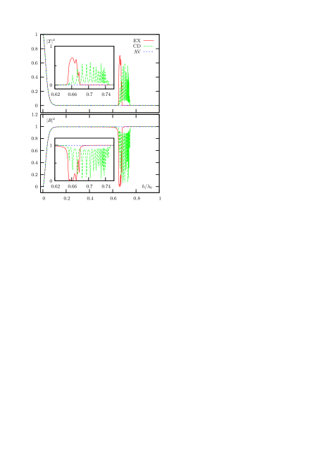
Figure 15: Same as in Fig. 5 but for Example B.

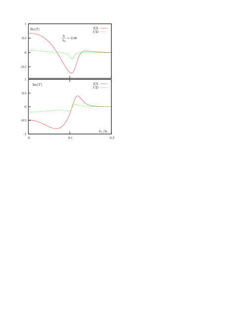
Figure 16: Example B. Real (top) and imaginary (bottom) parts of $T$ as functions of $k_{x}/k_{0}$ for $h/\lambda_{0}=0.66$. EX - exact result, CD - current-driven homogenization. Only the range of $k_{x}/k_{0}$ is shown for which $T$ computed by either method is not negligibly small.

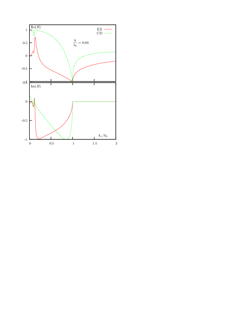
Figure 17: Example B. Same as in Fig. 16 but for $R$.

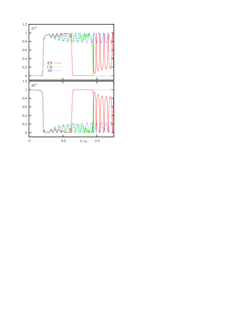
Figure 18: Example C. Same as in Fig. 5 but for Example C. Note that, in Example C, $h$ is fixed while $\lambda_{0}$ varies.

V.3 Example C

In this example, we consider spectral dependencies of $|R|^{2}$ and $|T|^{2}$ at normal incidence with the account of frequency dispersion in the constituents of the composite. The $a$-type medium is an idealized Drudean metal described by the permittivity function

$$\epsilon_{a}=\epsilon_{0}-\frac{\omega_{p}^{2}}{\omega(\omega+i\gamma)}\ .$$ (39)

and the $b$-type medium is vacuum or air. The sample consists of $N=10$ symmetric unit cells of the type $(a/2,b,a/2)$, where, again, $a=b$. We have chosen the parameters in (39) to represent the experimental values for silver: $\epsilon_{0}=5$ and $\omega_{p}/\gamma=500$. The lattice period $h$ is fixed so that $h/\lambda_{p}=0.2$, where $\lambda_{p}=2\pi c/\omega_{p}$ is the wavelength at the plasma frequency $\omega_{p}$. In the case of silver, $\lambda_{p}=136{\rm nm}$ so that $h\approx 27{\rm nm}$. The free-space wavelength $\lambda_{0}$ is varied. In this case, all physical quantities of interest can be expressed as functions of the dimensionless variables $h/\lambda_{0}$, $\lambda_{0}/\lambda_{p}$ and $k_{x}/k_{0}$ (we will take $k_{x}=0$ in this example).

We do not display the effective parameters obtained by different methods as nothing qualitatively new compared to the previously considered examples emerges in Example C. Note that the current-driven permeability $\mu_{xx}$ experiences a sharp resonance at $h/\lambda_{0}\approx 0.38$ while $\epsilon_{yy}$ and $\mu_{zz}$ do not exhibit any dramatic features. In Fig. 18, we plot $|T|^{2}$ and $|R|^{2}$ for $\lambda_{p}/\lambda_{0}$ varying from $0$ to $2.5$. The corresponding parameter $h/\lambda_{0}$ varies from $0$ to $0.5$. Again, the data clearly demonstrate that current-driven homogenization does not provide a meaningful correction to the standard result.

VI Bloch-wave analysis of the current-driven homogenization theory

In this section, we consider the current-driven homogenization theory from a more general point of view. We assume that the medium is intrinsically-nonmagnetic, three-dimensional and periodic, and that its true permittivity function $\tilde{\epsilon}({\bf r})$ satisfies the periodicity condition (1). Any such function can be expanded into a Fourier series

$$\tilde{\epsilon}({\bf r})=\sum_{\bf g}\epsilon_{\bf g}e^{i{\bf g}\cdot{\bf r}}\ ,$$ (40)

where

$${\bf g}=2\pi\left(\frac{\hat{\bf x}n_{x}}{h_{x}}+\frac{\hat{\bf y}n_{y}}{h_{y}}+\frac{\hat{\bf z}n_{z}}{h_{z}}\right)\ .$$

are the reciprocal lattice vectors, which can be viewed as three-dimensional summation indices, and $n_{x}$, $n_{y}$ and $n_{z}$ are arbitrary integers. We can seek the solution to (3) in the form of a Bloch wave

$${\bf E}({\bf r})=\sum_{\bf g}{\bf E}_{\bf g}e^{i({\bf k}+{\bf g})\cdot{\bf r}}\ .$$

The displacement ${\bf D}({\bf r})=\tilde{\epsilon}({\bf r}){\bf E}({\bf r})$ can be similarly expanded. Given the periodicity of $\tilde{\epsilon}({\bf r})$ expressed in (40), we can find the relation between the expansion coefficients ${\bf D}_{\bf g}$ and ${\bf E}_{\bf g}$:

$${\bf D}_{\bf g}=\sum_{\bf p}\epsilon_{\bf p}{\bf E}_{{\bf g}-{\bf p}}\ .$$ (41)

Upon substitution of the expansions into (3), we find the following system of equations for ${\bf E}_{\bf g}$:

$$({\bf k}+{\bf g}) \times ({\bf k}+{\bf g})\times{\bf E}_{\bf g}$$ (42)

$$+ k_{0}^{2}\left[\sum_{\bf p}\epsilon_{\bf p}{\bf E}_{{\bf g}-{\bf p}}+{\bf J}\delta_{{\bf g}0}\right]=0\ .$$

Equations of this kind are well known in the theory of photonic crystals Joannopoulos et al. (1995); Sakoda (2005), except that here we have included the free term ${\bf J}\delta_{{\bf g}0}$. However, the following analysis (proposed by us earlier Markel and Schotland (2012)) is rarely used.

Let us write (42) for the special cases ${\bf g}=0$ and ${\bf g}\neq 0$ separately. We note that ${\bf E}_{0}={\bf E}_{\rm av}$, where the low-pass filtered averages are defined in (5), and $\epsilon_{0}$ is the usual arithmetic average of $\tilde{\epsilon}({\bf r})$ (without low-pass filtering). We thus obtain:

$$\underline{{\bf g}=0\ :}$$ (43a)

$${\bf k}\times{\bf k}\times{\bf E}_{\rm av}+k_{0}^{2}\left[\epsilon_{0}{\bf E}_{\rm av}+\sum_{{\bf p}\neq 0}\epsilon_{\bf p}{\bf E}_{-{\bf p}}+{\bf J}\right]=0\ ,$$

$$\underline{{\bf g}\neq 0\ :}$$ (43b)

$$({\bf k}+{\bf g})\times({\bf k}+{\bf g})\times{\bf E}_{\bf g}+k_{0}^{2}\left[\sum_{{\bf p}\neq{\bf g}}\epsilon_{\bf p}{\bf E}_{{\bf g}-{\bf p}}+\epsilon_{\bf g}{\bf E}_{\rm av}\right]=0\ .$$

Note that only the first of these two equations is affected by our choice to include the external current in (3). We now utilize the linearity of equation (43b), from which we can write:

$$\sum_{{\bf p}\neq 0}\epsilon_{\bf p}{\bf E}_{-{\bf p}}=\left[\Sigma(\omega,{\bf k})-\epsilon_{0}\right]{\bf E}_{\rm av}\ ,$$ (44)

where $\Sigma(\omega,{\bf k})$ is a tensor to be determined by solving (43b). Here the factor $\epsilon_{0}$ (the average permittivity of the composite) has been introduced for convenience and does not result in any loss of generality. Then the ${\bf g}=0$ equation (43a) takes the following form:

$${\bf k}\times{\bf k}\times{\bf E}_{\rm av}+k_{0}^{2}\left[\Sigma(\omega,{\bf k}){\bf E}_{\rm av}+{\bf J}\right]=0\ .$$ (45)

This is, essentially, the same equation as (7). Consequently, $\Sigma(\omega,{\bf k})$ is the same tensor as the one appearing in the current-driven homogenization theory.

We note that inclusion into Maxwell’s equations of the external current (2) is not needed to compute $\Sigma(\omega,{\bf k})$, which is completely defined by the infinite set of equations (43b). We can refer to this set as to the cell problem. In what follows, we assume that the cell problem can be solved by means of linear algebra and that the tensor $\Sigma(\omega,{\bf k})$ can be computed.

Since $\Sigma(\omega,{\bf k})$ is defined completely by solving the cell problem, it is useful to consider what would happen if we set ${\bf J}=0$ in (45). Obviously, this would result in an eigenproblem

$$\left[\left({\bf k}\times{\bf k}\times\right)+k_{0}^{2}\Sigma(\omega,{\bf k})\right]{\bf E}_{\rm av}=0\ .$$ (46)

The above equation has nontrivial solutions only when ${\bf k}={\bf q}$, where the Bloch wave vector ${\bf q}$ is determined from the equation

$${\rm det}\left[\left({\bf k}\times{\bf k}\times\right)+k_{0}^{2}\Sigma(\omega,{\bf k})\right]=0\ .$$ (47)

The solution to this equation, viewed as a function of frequency, yields the dispersion equation of the medium, ${\bf q}={\bf q}(\omega)$. The dispersion relation is physically measurable and the same is true for the on-shell tensor $\Sigma(\omega,{\bf q})$. For example, in the simplest case of transverse waves, the dispersion equation takes the form $q^{2}=k_{0}^{2}\Sigma(\omega,{\bf q})$ and the quantity $\Sigma(\omega,{\bf q})$ can be referred to as the propagation constant (index of refraction squared) of the Bloch mode Menzel et al. (2010); Alaee et al. (2013).

We can seek approximate solutions to (47) by using the limit ${\bf k}\rightarrow 0$. As was discussed in Sec. II.2, the tensor $\Sigma(\omega,{\bf k})$ can be formally expanded in a non-gyrotropic medium according to (13). We substitute this expansion into (47) and obtain

$${\rm det}\left[\left({\bf k}\times(1-\beta){\bf k}\times\right)+k_{0}^{2}\Sigma(\omega,0)\right]=0\ .$$ (48)

Equation (48) is a valid approximation to the dispersion equation in the weak nonlocality regime and its solution yields the first nonvanishing solution to ${\bf q}$ (compared to the limit $h\rightarrow 0$). Also, (48) coincides with the dispersion equation in a homogeneous medium with local parameters $\epsilon=\Sigma(\omega,0)$ and $\mu=(1-\beta)^{-1}$. If we make this identification, we would arrive at the same homogenization result as in the current-driven homogenization theory, except that we did not need to introduce the external current. However, this identification is not mathematically justified due to the reasons already discussed by us in Sec. II.2. Here we reiterate these arguments in the somewhat new light of the Bloch-wave analysis.

Firstly and most importantly, it can be easily seen that multiplication of (48) by a scalar $\xi$ does not alter the dispersion equation or the value of ${\bf q}$ but doing so does alter the impedance ${\mathscr{Z}}$. Therefore, the above procedure is not expected to yield a meaningful correction to ${\mathscr{Z}}$. This was illustrated above in Fig. 11. In fact, S-parameter retrieval predicts a much more accurate ${\mathscr{Z}}$ while keeping approximately the same dispersion relation. This was illustrated in Fig. 7. And in general, it could not be reasonably expected that a theory that considers infinite media and disregards the physical boundary would predict the impedance correctly.

Second, the procedure described above is clearly inapplicable outside of the weak nonlocality regime and, in particular, when $\|\beta\|\sim 1$. In this region of parameters, introduction of the local permittivity and permeability tensors does not result in a correct dispersion relation, even approximately. But this is exactly the region of parameters where current-driven homogenization predicts magnetic resonances. Consequently, this prediction is mathematically unjustified.

VII Discussion

VII.1 Current-driven excitation model and the theory of nonlocality

The current-driven homogenization theory is deeply rooted in the theory of natural electromagnetic nonlocality (spatial dispersion) Agranovich and Ginzburg (1966); Landau and Lifshitz (1984). The latter is, of course, a very successful theory, which has predicted and described theoretically such diverse phenomena as optical activity, additional waves, and anisotropy of crystals with cubic symmetry, etc. However, current-driven homogenization and, more generally, current-driven excitation model take certain analogies too far or apply them unscrupulously.

The basic idea behind the current-driven excitation model can be traced to Ref. Agranovich and Ginzburg, 1966. We translate the relevant text from the Russian edition of this book (Moscow, Nauka, 1965, p. 34), using only a slight change of notations:

“Generally, the arguments of the tensor $\Sigma(\omega,{\bf k})$ are mathematically-independent. This fact follows already from the definition (1.6) [equivalent to Eqs. 49,50 below (authors’ comment)] but can be at times not entirely obvious. This is so because, in optics, one encounters very frequently wave propagation in the absence of sources in the medium itself, in which case ${\bf k}$ is a function of $\omega$; for example, for normal homogeneous plane waves, ${\bf k}=(\omega/c)\tilde{n}(\omega,\hat{\bf s})\hat{\bf s}$. But if ${\bf k}={\bf k}(\omega)$, then the spatial dispersion appears to be indistinguishable from the frequency dispersion. This observation raises a question [about the physical nature of spatial nonlocality (authors’ comment)] and the answer to this question is the following. The tensor $\Sigma(\omega,{\bf k})$ is introduced for fields of the most general form, obtained when the sources ${\bf J}_{\rm ext}({\bf r})$ and $\rho_{\rm ext}({\bf r})$ spatially overlap with the medium. Under these conditions, it is possible to create a field ${\bf E}$ with arbitrary and mathematically independent $\omega$ and ${\bf k}$ (the Fourier components $\tilde{\bf E}(\omega,{\bf k})$ is ultimately expressed in terms of ${\bf J}_{\rm ext}(\omega,{\bf k})$ and $\rho_{\rm ext}(\omega,{\bf k})$; see $2.1). From this, it follows immediately that all problems involving wave propagation can be solved if $\Sigma(\omega,{\bf k})$ is known.”

The last sentence in the above is only partially correct. In the case of natural nonlocality, $\Sigma(\omega,{\bf k})$ is the spatial Fourier transform of the influence function $\sigma(\omega;{\bf r},{\bf r}^{\prime})$, which appears in the nonlocal relation between ${\bf D}(\omega,{\bf r})$ and ${\bf E}(\omega,{\bf r})$, viz,:

$${\bf D}(\omega,{\bf r})=\int_{V}\sigma(\omega;{\bf r},{\bf r}^{\prime}){\bf E}(\omega,{\bf r}^{\prime})d^{3}r^{\prime}\ .$$ (49)

If both points ${\bf r}$ and ${\bf r}^{\prime}$ are sufficiently far from the boundary of the medium, we can write $\sigma(\omega;{\bf r},{\bf r}^{\prime})=f(\omega,{\bf r}-{\bf r}^{\prime})$. Then $\Sigma(\omega,{\bf k})$ is defined as the spatial Fourier transform of $f(\omega,{\bf r})$:

$$\Sigma(\omega,{\bf k})=\int f(\omega,{\bf r})e^{i{\bf k}\cdot{\bf r}}d^{3}r\ .$$ (50)

But this is insufficient to solve the boundary-value problem for any finite shape. To that end, we would need to know how $\sigma(\omega;{\bf r},{\bf r}^{\prime})$ behaves when at least one of the points ${\bf r}$ and ${\bf r}^{\prime}$ is close to the boundary. One can consider an approximation of the type

$$\sigma(\omega;{\bf r},{\bf r}^{\prime}) = S({\bf r})f(\omega,{\bf r}-{\bf r}^{\prime})S({\bf r}^{\prime})$$ (51)

$$+ [1-S({\bf r})]\delta({\bf r}-{\bf r}^{\prime})[1-S({\bf r}^{\prime})]\ ,$$

where $S({\bf r})$ is the shape function: it is equal to unity inside the medium and to zero outside (in vacuum). If (51) holds, then the statement under consideration is correct: Maxwell’s equations can be written in a closed form using only the Fourier transform of $f(\omega,{\bf r})$ and the Fourier transform of the shape function. Therefore, if $\Sigma(\omega,{\bf k})$ is known, then Maxwell’s equations can be solved in a finite sample, at least in principle. We note that the familiar relation ${\bf D}(\omega,{\bf k})=\Sigma(\omega,{\bf k}){\bf E}(\omega,{\bf k})$ does not hold in this case and Maxwell’s equations, written in the ${\bf k}$-domain, contain an integral transform and cannot be solved by algebraic manipulation. This difficulty is known and explained in $ 10 of Ref. Agranovich and Ginzburg, 1966 but appears to be scarcely appreciated in the modern literature. But regardless of this difficulty, there is no reason to believe that (51) is generally true. This approximation can be applicable, perhaps, if the nonlocal interaction between two points is transmitted only along the line of sight and if the body is convex. However, the first of these assumptions is difficult to justify.

The same analysis applies to current-driven homogenization of periodic composites. The knowledge of the function $\Sigma(\omega,{\bf k})$, as defined by (5) or by (44), allows one to find the law of dispersion but is insufficient to solve any boundary value problem. Therefore, this function is not an intrinsic physical characteristic of a composite. It is, rather, an auxiliary mathematical function, which appears when a certain ansatz is substituted into Maxwell’s equations written for an infinite periodic medium.

Now the difference between the classical theory of nonlocality and the current-driven homogenization theory becomes apparent. In the former case, the real-space influence function $\sigma(\omega;{\bf r},{\bf r}^{\prime})$ is derived from first principles (e.g., from a microscopic theory) or introduced phenomenologically and then it completely characterizes the electromagnetic properties of a macroscopic object of any shape in the sense that it renders Maxwell’s equations closed. As discussed above, under some limited conditions, the dependence of $\sigma(\omega;{\bf r},{\bf r}^{\prime})$ on the two variables ${\bf r}$ and ${\bf r}^{\prime}$ can be simplified, e.g., as in (51), and then there exists a one-to-one correspondence between $\sigma(\omega;{\bf r},{\bf r}^{\prime})$ and $\Sigma(\omega,{\bf k})$. But in the case of current-driven homogenization theory, the low-pass filtering (5) does not follow from any first principle. Moreover, if (5) is accepted as the fundamental definition of $\Sigma(\omega,{\bf k})$, there is no way to establish a one-to-one correspondence between the latter and the real-space function $\sigma(\omega;{\bf r},{\bf r}^{\prime})$. As a result, the knowledge of $\Sigma(\omega,{\bf k})$, thus defined, is insufficient to solve a boundary-value problem in any finite sample.

Another obvious distinction between the two theories is that, for natural nonlocality, the influence range (the characteristic value of $|{\bf r}-{\bf r}^{\prime}|$ for which $\sigma(\omega;{\bf r},{\bf r}^{\prime})$ is not negligibly small) is of the order of the atomic scale. Therefore, in the optical range, the condition of weak nonlocality is satisfied with extremely good precision and all the effects of nonlocality are, essentially, small perturbations. In the case of current-driven homogenization, the influence range is $h$ and the effects claimed as a result of current-driven homogenization (e.g., $\mu\approx-1$) are dramatic and nonperturbative.

So far, we have discussed the physical and mathematical meaning of the function $\Sigma(\omega,{\bf k})$ as it is used both in the theory of natural nonlocality and in current-driven homogenization. The next important point to consider is the unjustified assumption of the current-driven homogenization theory (and, more generally, of the current-driven excitation model) that the external current of the form (2) can, under some unspecified conditions, be created in the medium. This assumption also grows conceptually from the above quote. In reality, “wave propagation in the absence of sources in the medium itself” is encountered in optics (and, more generally, in macroscopic electrodynamics) not just “very frequently,” but always, without any known exceptions. Of course a medium can be optically active and emit some kind of radiation from its volume. However, in all such cases, the current inside the medium is subject to (linear or nonlinear) constitutive relations and cannot be created or controlled by an experimentalist at will.

Finally, another relevant misconception, which has been widely popularized in recent years Agranovich et al. (2004, 2006); Agranovich and Gartstein (2006, 2009), is the proposition of equivalence of weak nonlocality of the dielectric response and nontrivial magnetic permeability. We have discussed this point in this article in much detail and have demonstrated that the equivalence exists only for the dispersion relation but not for the impedance of the medium. It can be argued that this is exactly what was meant by Landau and Lifshitz Landau and Lifshitz (1984) since none of the relevant chapters consider boundary conditions in any form. The current-driven homogenization theory has taken this statement of equivalence out of its proper context and applied it to the problem of homogenization wherein the boundary conditions play the central role.

It can be concluded that the classical theory of spatial dispersion is concerned primarily with certain physical effects such as rotation of the plane of polarization or appearance of additional waves, which are not present in the purely local regime but can be described as perturbations if small nonlocal corrections to the permittivity tensor are taken into account. The corrections are either introduced phenomenologically or computed using a microscopic theory. The theory of spatial dispersion was never meant to be used for rigorous solution of boundary value problems and, therefore, the discussion of the dispersion equation sufficed in the vast majority of cases. For this reason, certain remarks appearing in the classical texts on the subject, such as the now famous remark of Landau and Lifshitz regarding the equivalence of nonlocality and magnetism, apply only to the dispersion relation. In the case of the current-driven homogenization theory, all these limitations have been disregarded.

VII.2 Homogenization by spatial Fourier transform

Throughout the paper, we have emphasized the critical importance of taking the boundary effects into account in electromagnetic homogenization, particularly in the case of metamaterials whose lattice cell size typically constitutes an appreciable fraction of the vacuum wavelength. Consequently, theories relying entirely on the bulk behavior of waves cannot be accurate; they may be capable of finding the effective index but not the impedance. We note that the role of boundary conditions has been elucidated and emphasized in the literature previously Simovski (2009); Felbacq (2000); however, in this work, we have presented a detailed case study using an exactly solvable model.

Generally speaking, Fourier-based homogenization theories should be applied with extreme care because Fourier analysis makes it difficult to account for material interfaces, which break the discrete translational invariance of a periodic composite.

It is feasible to devise a theory in which Fourier analysis is applied in the medium and in the empty space separately. In this case, however, only natural Bloch modes will exist in the material, and no other values of ${\bf k}$ will appear. The intuitive perception that a small localized source (e.g., a nano-antenna) embedded in a composite (e.g., in one of the empty voids) would generate within the material the whole spectrum of waves with all possible real-valued ${\bf k}$’s is correct only in a very narrow technical sense. In fact, within any area away from the small source, the waves with various ${\bf k}$ will interfere to produce the natural Bloch modes of the periodic structure. Only the latter are physically measurable.

VII.3 Current-driven homogenization

As an illustration of the general principles stated above, we have critically analyzed the current-driven homogenization theory of Refs. Silveirinha, 2007; Alu, 2011, which does not account for the boundaries of the medium but derives the effective parameters from the behavior of waves in the bulk. In addition, this model relies on the use of physically-unrealizable sources inside the medium, with no justification as to why the results thus obtained should be experimentally relevant.

The numerical results of Sec. V are therefore not surprising. They demonstrate that current driven homogenization does not yield accurate results in the range of parameters where it predicts nontrivial magnetic effects. In particular, the errors of the transmission and reflection coefficients $T$ and $R$ are of the same order of magnitude or, in some cases, much larger than the deviation of the magnetic permeability from unity, $\|\mu-1\|$, where $\mu$ is the local permeability tensor predicted by current-driven homogenization.

In most cases considered, current-driven homogenization does not provide a noticeable improvement in accuracy compared to the standard homogenization result (16). In the cases when such improvement can be observed, e.g., in Fig. 5, this is due to a correction in the effective permittivity $\epsilon$ rather than to an accurate prediction of $\mu$. We note in passing that the correction to the magnetic permeability produced by the current-driven model is asymptotically $\mathcal{O}(kh)^{4}$, which is different from the $\mathcal{O}(kh)^{2}$ asymptote that follows from S-parameter retrieval.

VIII Summary

This paper has three main conclusions.

First, careful consideration of boundary conditions is required in all effective medium theories (EMTs).

Second, all EMTs have an applicability range, and wherever a homogenization result is obtained, it is important to verify that the parameters of the composite are within this range or, otherwise, validate the result with direct simulation.

Third, there are many EMTs that yield the standard homogenization result in the limit $h\rightarrow 0$ but different $h$-dependent corrections to the former. Validating that these corrections are physically meaningful requires consideration of finite samples and cannot be done by investigating an infinite periodic composite (this conclusion is closely related to the first one).

Appendix A Determination of the coefficients ${\mathscr{A}}_{a}$, ${\mathscr{B}}_{a}$, ${\mathscr{A}}_{b}$ and ${\mathscr{B}}_{b}$ from the boundary conditions

Upon substitution of the expressions (20) into (21), we obtain the following set of linear equations:

$$e^{-i\theta_{a}}\Big{(}e^{i\phi_{a}}A_{a}+e^{-i\phi_{a}}B_{a}\Big{)}+\Big{(}A_{b}+B_{b}\Big{)}=1\ ,$$

$$\frac{\kappa_{a}}{q_{z}}e^{-i\theta_{a}}\Big{(}e^{i\phi_{a}}A_{a}-e^{-i\phi_{a}}B_{a}\Big{)}+\frac{\kappa_{b}}{q_{z}}\Big{(}A_{b}-B_{b}\Big{)}=1\ ,$$

$$\Big{(}A_{a}+B_{a}\Big{)}+e^{-i\theta_{b}}\Big{(}e^{i\phi_{b}}A_{b}+e^{-i\phi_{b}}B_{b}\Big{)}=1\ ,$$

$$\frac{\kappa_{a}}{q_{z}}\Big{(}A_{a}-B_{a}\Big{)}+\frac{\kappa_{b}}{q_{z}}e^{-i\theta_{b}}\Big{(}e^{i\phi_{b}}A_{b}-e^{-i\phi_{b}}B_{b}\Big{)}=1\ .$$

This set is somewhat more complicated than what is encountered in the ordinary theory of one-dimensional photonic crystals. In the latter case, the matrix is the same but the right-hand side is zero. Correspondingly, the task is to find the value of $k_{z}$ (for a given $k_{x}$) such that the equations have a nontrivial solution. This occurs when $k_{z}=q_{z}$, where $q_{z}$ is defined in Eq. (24). In this manner, the natural Bloch wave vector ${\bf q}$ of the medium is determined. For the case at hand, both $k_{x}$ and $k_{z}$ are free parameters but the right-hand side is nonzero. Therefore, the current-driven homogenization theory, essentially, replaces the problem of funding the natural Bloch mode of the medium by a mathematically unrelated problem of inverting the matrix in the above set of equations.

The solution to the set stated above is given by (22) where ${\mathscr{D}}$ is defined in (23) and

$${\mathscr{A}}_{a}=e^{\frac{i}{2}(\theta_{a}-\phi_{a})}\left\{\left(1+\frac{q_{z}}{\kappa_{a}}\right)\left[\cos\left(\theta_{b}+\frac{\theta_{a}+\phi_{a}}{2}\right)\right.\right.$$

$$\left.\left.-\cos\phi_{b}\cos\frac{\theta_{a}+\phi_{a}}{2}\right]+\left(\frac{\kappa_{b}}{\kappa_{a}}+\frac{q_{z}}{\kappa_{b}}\right)\sin\phi_{b}\sin\frac{\theta_{a}+\phi_{a}}{2}\right\}\ ,$$

$${\mathscr{B}}_{a}=e^{\frac{i}{2}(\theta_{a}+\phi_{a})}\left\{\left(1-\frac{q_{z}}{\kappa_{a}}\right)\left[\cos\left(\theta_{b}+\frac{\theta_{a}-\phi_{a}}{2}\right)\right.\right.$$

$$\left.\left.-\cos\phi_{b}\cos\frac{\theta_{a}-\phi_{a}}{2}\right]-\left(\frac{\kappa_{b}}{\kappa_{a}}-\frac{q_{z}}{\kappa_{b}}\right)\sin\phi_{b}\sin\frac{\theta_{a}-\phi_{a}}{2}\right\}\ ,$$

$${\mathscr{A}}_{b}=e^{\frac{i}{2}(\theta_{b}-\phi_{b})}\left\{\left(1+\frac{q_{z}}{\kappa_{b}}\right)\left[\cos\left(\theta_{a}+\frac{\theta_{b}+\phi_{b}}{2}\right)\right.\right.$$

$$\left.\left.-\cos\phi_{a}\cos\frac{\theta_{b}+\phi_{b}}{2}\right]+\left(\frac{\kappa_{a}}{\kappa_{b}}+\frac{q_{z}}{\kappa_{a}}\right)\sin\phi_{a}\sin\frac{\theta_{b}+\phi_{b}}{2}\right\}\ ,$$

$${\mathscr{B}}_{b}=e^{\frac{i}{2}(\theta_{b}+\phi_{b})}\left\{\left(1-\frac{q_{z}}{\kappa_{b}}\right)\left[\cos\left(\theta_{a}+\frac{\theta_{b}-\phi_{b}}{2}\right)\right.\right.$$

$$\left.\left.-\cos\phi_{a}\cos\frac{\theta_{b}-\phi_{b}}{2}\right]-\left(\frac{\kappa_{a}}{\kappa_{b}}-\frac{q_{z}}{\kappa_{a}}\right)\sin\phi_{a}\sin\frac{\theta_{b}-\phi_{b}}{2}\right\}\ .$$

It can be seen that ${\mathscr{B}}_{a}$ is obtained from ${\mathscr{A}}_{a}$ (or vice versa) by changing the signs of the propagation constants $\kappa_{a}$ and $\kappa_{b}$ and of the related phases $\phi_{a}$ and $\phi_{b}$ (but not of $\theta_{a}$ and $\theta_{b}$), and similarly for the pair of coefficients ${\mathscr{A}}_{b}$, ${\mathscr{B}}_{b}$. Also, the coefficients are invariant under the the permutation of indices $a\leftrightarrow b$.

Appendix B Closed-form expressions for effective medium parameters obtained by current-driven homogenization

In this Appendix we give the closed-form solution for the general case $a\neq b$. If $a=b$, these expressions are significantly simplified. However, in the numerical codes used to produce the figures for this paper, we have used the general expressions given below.

In addition to (15) and (16), we need to introduce the following notations:

• The phase shifts $\phi_{a}$ and $\phi_{b}$ computed at $k_{x}=0$ are denoted by $\psi_{a}$ and $\psi_{b}$:

  $$\psi_{a}=\left.\phi_{a}\right|_{k_{x}=0}=k_{a}a\ ,\ \ \psi_{b}=\left.\phi_{b}\right|_{k_{x}=0}=k_{b}b\ .$$

• The refractive indices of each layer are denoted by $n_{a}=\sqrt{\epsilon_{a}}$ and $n_{b}=\sqrt{\epsilon_{b}}$. The branches of all square roots are defined by the condition $0\leq{\rm arg}(\sqrt{z})<\pi$.

• The dimensional size parameters for the lattice:

  $$x_{a}=k_{0}a\ ,\ \ x_{b}=k_{0}b\ ,\ \ x=x_{a}+x_{b}=k_{0}h\ .$$

  Note that $\psi_{a}=n_{a}x_{a}$, $\psi_{b}=n_{b}x_{b}$.

• The following symmetric combinations of the trigonometric functions:

  $$\alpha_{1}=2\left(n_{a}\sin\psi_{a}+n_{b}\sin\psi_{b}\right)\ ,$$

  $$\alpha_{2}=2\left(n_{a}\epsilon_{b}\sin\psi_{a}+n_{b}\epsilon_{a}\sin\psi_{b}\right)\ ,$$

  $$\alpha_{3}=x_{a}\cos\psi_{a}+x_{b}\cos\psi_{b}\ ,$$

  $$\alpha_{4}=x_{b}^{2}n_{a}\sin\psi_{a}+x_{a}^{2}n_{b}\sin\psi_{b}\ ,$$

  and

  $$\xi_{1} =n_{a}\cos\frac{\psi_{a}}{2}\sin\frac{\psi_{b}}{2}+n_{b}\cos\frac{\psi_{b}}{2}\sin\frac{\psi_{a}}{2}\ ,$$

  $$\xi_{2} =n_{a}\cos\frac{\psi_{b}}{2}\sin\frac{\psi_{a}}{2}+n_{b}\cos\frac{\psi_{a}}{2}\sin\frac{\psi_{b}}{2}\ ,$$

  $$\xi_{3} =n_{a}\sin\psi_{a}\cos\psi_{b}+n_{b}\sin\psi_{b}\cos\psi_{a}\ ,$$

  $$\xi_{4} =n_{a}n_{b}\frac{\epsilon_{a}+\epsilon_{b}}{2}\left(\psi_{a}\sin\psi_{a}\cos\psi_{b}+\psi_{b}\sin\psi_{b}\cos\psi_{a}\right)$$

  $$+\epsilon_{a}\epsilon_{b}\left(\psi_{b}\sin\psi_{a}\cos\psi_{b}+\psi_{a}\sin\psi_{b}\cos\psi_{a}\right)\ ,$$

  $$\xi_{5} =(\epsilon_{a}-\epsilon_{b})^{2}\sin\frac{\psi_{a}}{2}\sin\frac{\psi_{b}}{2}\ ,$$

  and

  $$\eta =\epsilon_{a}(2+\cos\psi_{b})\sin^{2}\frac{\psi_{a}}{2}+\epsilon_{b}(2+\cos\psi_{a})\sin^{2}\frac{\psi_{b}}{2}$$

  $$+n_{a}n_{b}\sin\psi_{a}\sin\psi_{b}\ ,$$

  $$\zeta =\epsilon_{a}\left(4\psi_{b}\epsilon_{b}-\psi_{b}\epsilon_{a}+3\psi_{a}n_{a}n_{b}\right)\sin^{2}\frac{\psi_{a}}{2}\sin\psi_{b}$$

  $$+\epsilon_{b}\left(4\psi_{a}\epsilon_{a}-\psi_{a}\epsilon_{b}+3\psi_{b}n_{a}n_{b}\right)\sin^{2}\frac{\psi_{b}}{2}\sin\psi_{a}$$

  $$+8(\epsilon_{a}-\epsilon_{b})^{2}\sin^{2}\frac{\psi_{a}}{2}\sin^{2}\frac{\psi_{b}}{2}$$

  $$-\left(\psi^{2}_{a}\epsilon^{2}_{b}\sin^{2}\frac{\psi_{b}}{2}+\psi^{2}_{b}\epsilon^{2}_{a}\sin^{2}\frac{\psi_{a}}{2}\right)\ ,$$

  and the following combinations of the functions introduced above:

  $$\sigma =\epsilon_{a}\epsilon_{b}(\alpha_{4}-4\alpha_{3})-\alpha_{2}\ ,$$

  $$\tau =4\left(\xi_{3}\xi_{5}+\xi_{2}\xi_{4}\right)\ .$$

  Note that by symmetry we mean here invariance with respect to permutation of indexes $a\leftrightarrow b$.

Then the cosed-form expressions for the current-driven effective parameters of the layered medium considered in this paper can be stated as follows [we adduce the expressions for $\beta_{xx}$ and $\beta_{zz}$; $\mu_{xx}$ and $\mu_{zz}$ are given by (30)]:

$$\epsilon_{yy}=\frac{x}{Z}(\epsilon_{a}\epsilon_{b})^{2}{\mathscr{D}}_{0}\ ,$$

$$\beta_{xx}=\frac{2\xi_{1}^{2}}{Z^{2}}(\epsilon_{b}-\epsilon_{a})^{2}\left[\zeta-x^{2}p_{a}p_{b}\epsilon_{a}\epsilon_{b}\eta\right]\ ,$$

$$\beta_{zz}=-\frac{\xi_{1}}{Z^{2}}(\epsilon_{b}-\epsilon_{a})^{2}$$

$$\times\left\{n_{a}n_{b}\left[2\rho+x\xi_{2}(\sigma-\alpha_{1}\epsilon_{\parallel})\right]-2\alpha_{1}\xi_{5}+\tau\right\}\ ,$$

where

$$Z=x\frac{(\epsilon_{a}\epsilon_{b})^{2}}{\epsilon_{\perp}}{\mathscr{D}}_{0}-4\xi_{1}\xi_{5}$$

and ${\mathscr{D}}_{0}$ is the determinant (23) evaluated at ${\bf k}=0$:

$${\mathscr{D}}_{0} =1-\left.\cos(q_{z}h)\right|_{k_{x}=0}$$

$$=1-\cos\psi_{a}\cos\psi_{b}+\frac{1}{2}\left(\frac{n_{a}}{n_{b}}+\frac{n_{b}}{n_{a}}\right)\sin\psi_{a}\sin\psi_{b}\ ,$$

and, finally,

$$\rho =\epsilon_{a}\epsilon_{b}\xi_{2}x^{2}(2+p_{a}p_{b}{\mathscr{D}}_{0})$$

$$-n_{a}n_{b}x\sin\frac{\psi_{a}}{2}\sin\frac{\psi_{b}}{2}\left(\epsilon_{a}\epsilon_{b}x^{2}+2\epsilon_{\parallel}{\mathscr{D}}_{0}\right)\ .$$

Appendix C S-parameter retrieval techniques used in this paper

S-parameter retrieval is a well-established technique. However, the vast majority of papers that consider S-parameter retrieval are focused on normal incidence only. This limitation does not allow one to access all tensor elements of the effective parameters. In this Appendix, we will remove this limitation and include off-normal incidences into consideration.

Consider an anisotropic homogeneous slab characterized by the tensors $\epsilon={\rm diag}(\epsilon_{\perp},\epsilon_{\perp},\epsilon_{\parallel})$ and $\mu={\rm diag}(\mu_{\perp},\mu_{\perp},\mu_{\parallel})$. The transmission and reflection coefficients are given in Sec. IV. It is convenient to rewrite the expressions given in that section in the following form:

$$T=\frac{4pC}{(C+1)^{2}-p^{2}(C-1)^{2}}\ ,$$ (52a)

$$R=\frac{(1-p)^{2}(C^{2}-1)}{(C+1)^{2}-p^{2}(C-1)^{2}}\ .$$ (52b)

Here

$$C=\frac{q_{z}\eta_{\parallel}}{\kappa_{0}}\ ,\ \ p=\exp\left(iq_{z}L\right)\ .$$ (53)

We refer the reader to Sec. IV for relevant notations. Note the symmetries $R(p,C)=-R(p,1/C)$ and $T(p,C)=T(p,1/C)$.

If $T$ and $R$ are known at some incidence angle (parameterized by $k_{x}$), so are $C$ and $p$. The expressions for $C$ and $p$ in terms of $T$ and $R$ [inversion of (52)] is unique up to the branch of a square root and widely known:

$$C=\frac{\pm D}{T^{2}-(1-R)^{2}}\ ,\ \ p=\frac{1+T^{2}-R^{2}\pm D}{2T}\ ,$$

where

$$D=\sqrt{(1+T^{2}-R^{2})^{2}-(2T)^{2}}\ .$$

In the case of low transmission (small $|T|$), one can use the approximate formulas

$$C=\ \ \frac{1+R}{1-R}\ ,\ \ p=\frac{T}{1-R^{2}}\ \ {\rm(first\ branch)}\ ,$$

$$C=-\frac{1+R}{1-R}\ ,\ \ p=\frac{1-R^{2}}{T}\ \ {\rm(second\ branch)}\ .$$

Here we have encountered the first instance of a branch ambiguity, but it can be easily resolved by using the condition of medium passivity, $|p|<1$. Other than the branch ambiguity mentioned, the above inversion formulas (that yield $C$ and $p$ in terms of $T$ and $R$) are well-posed and stable and establish one-to-one correspondence between the complex pairs $(T,R)$ and $(C,p)$.

Given the above result, we can assume that $C(k_{x})$ and $p(k_{x})$ are known as functions of $k_{x}$ and seek effective tensors $\epsilon$ and $\mu$ that are consistent with these functions. In general, purely local tensors $\epsilon$ and $\mu$ that “reproduce” two given functions $C(k_{x})$ and $p(k_{x})$ may not exist. Therefore, we shall focus on a more narrow task of finding $\epsilon$ and $\mu$ that reproduce $C(k_{x})$ and $p(k_{x})$ at normal ($k_{x}=0$) and close-to-normal incidences.

It is well known that, if we consider normal incidence only (or any other fixed value of $k_{x}$), then the solution is not unique due to the branch ambiguity of the logarithm function. More specifically, the quantities $C$ and $p$ given by (53) are invariant with respect to the simultaneous transformation $q_{z}\rightarrow q_{z}+2\pi m/L$, $\eta_{\parallel}\rightarrow q_{z}/(q_{z}+2\pi m/L)$, where $m$ is an integer. We therefore will include both normal and off-normal incidences into consideration. Unfortunately, the problem is still ill-posed in this case. Generally, the retrieval problem can not be formulated as a well-posed system of equations. We shall now describe three different approaches to obtaining a solution to the retrieval problem that is optimal in the sense that it yields all relevant elements of the tensors $\epsilon$ and $\mu$ and reproduces the angular dependence $C(k_{x})$ and $p(k_{x})$ [or $T(k_{x})$, $R(k_{x})$] in as wide range of $k_{x}$ as possible.

In what follows, we wasume that the effective medium is a uniaxial crystal with $\epsilon={\rm diag}(\epsilon_{\parallel},\epsilon_{\parallel},\epsilon_{\perp})$ and $\mu={\rm diag}(\mu_{\parallel},\mu_{\parallel},\mu_{\perp})$. Also, the notations $\eta$ refers to $\mu$ for s-polarization and to $\epsilon$ for p-polarization.

Method 1

Let $t=k_{x}/k_{0}$ and $x=k_{0}L$. Given the dispersion equation (34), we can write

$$C(t)=\frac{\sqrt{1-t^{2}}\eta_{\parallel}}{Q(t)}\ ,\ \ p(t)=e^{ixQ(t)}\ ,$$ (54)

where

$$Q(t)=\sqrt{n^{2}-\frac{\eta_{\parallel}}{\eta_{\perp}}t^{2}}\ .$$

Here $n^{2}=\epsilon_{\parallel}\mu_{\parallel}$ is the squared index of refraction and recall that $\eta$ refers to $\mu$ for s-polarization and to $\epsilon$ for p-polarization.

Assuming $C(t)$ and $p(t)$ are known functions, we can express $Q(t)$ by inverting each equation in (54). This yields two solutions for $Q(t)$:

$$Q_{1}(t)=\frac{\eta_{\parallel}\sqrt{1-t^{2}}}{C(t)}\ ,\ \ Q_{2}(t)=\frac{1}{ix}\ln\left[p(t)\right]+\Delta m\ ,$$

where $\Delta=2\pi/x$ and $m$ an arbitrary integer.

If we could find such tensors $\epsilon$ and $\mu$ that $Q_{1}(t)=Q_{2}(t)$ for all values of $t$, then these parameters would describe transmission and reflection by the slab for all angles of incidence with perfect precision. This is possible only in the $h\rightarrow 0$ limit. Here we will require that the functions coincide at normal incidence and have the same second derivative with respect to $t$ (the first derivative is identically zero). To this end, it is convenient to introduce the functions

$$F(t)=\frac{1-t^{2}}{C(t)}\ ,\ \ G(t)=\frac{1}{ix}\ln\left[p(t)\right]\ .$$

Since these functions are expressed in terms of $C(t)$, $p(t)$ and known analytical functions (they do not contain any unknowns), we can view them as directly measurable (or computable in terms of $T$ and $R$). Then the main equation we wish to fit takes the form

$$\eta_{\parallel}F(t)=G(t)+\Delta m\ .$$

Here $\eta_{\parallel}$ and $m$ (the branch index) are the unknowns. Of course, this equation has no solutions in general. But we can require that it holds to second order in $t$ in the vicinity of $t=0$. We can expand $F(t)$ as

$$F(t)=F_{0}+F_{2}t^{2}\ ,\ \ F_{0}=F(0)\ ,\ \ F_{2}=\lim_{\tau\rightarrow 0}\frac{F(\tau)-F_{0}}{\tau^{2}}\ .$$

and similarly for $G(t)$. This results in a pair of algebraic equations

$$\eta_{\parallel}F_{0}=G_{0}+\Delta m\ ,$$

$$\eta_{\parallel}F_{2}=G_{2}\ .$$

Even though this is a system of two linear equations with respect to two unknowns, it still cannot be solved because $m$ is, by definition, integer. We can, however, solve the first equation exactly (this will guarantee the correct $T$ and $R$ at normal incidence) and then minimize the norm of the second equation. This results in the following inverse solution:

$$m={\rm Nint}\left[\frac{F_{0}G_{2}-G_{0}F_{2}}{\Delta F_{2}}\right]\ ,$$ (55a)

$$\eta_{\parallel}=\frac{G_{0}+\Delta m}{F_{0}}\ ,$$ (55b)

where ${\rm Nint}[z]$ denotes nearest integer to the real part of $z$. Note that the second expression in the above (for $\eta_{\parallel}$) must use the value of $m$ computed using the first equation.

Once the quantities $\eta_{\parallel}$ and $m$ are known, we can also compute the squared refractive index according to

$$n^{2}=(G_{0}+\Delta m)^{2}$$

Then, if $\eta_{\parallel}=\mu_{\parallel}$ (s-polarization), we can compute $\epsilon_{\parallel}=n^{2}/\eta_{\parallel}$. Otherwise, if $\eta_{\parallel}=\epsilon_{\parallel}$, we can compute $\mu_{\parallel}=n^{2}/\eta_{\parallel}$.

This Method 1 does not give access to $\epsilon_{\perp}$ and $\mu_{\perp}$. To obtain these tensor elements, Method 3 must be used.

Method 2

This method combines Method 1 with the main idea of Ref. Chen et al., 2004. Namely, starting from some sufficiently low frequency $\omega$ or some sufficiently small $h$, we gradually increase the relevant parameter ($\omega$ or $h$) and apply Method 1 at each iteration of this loop. However, after a few initial iterations, we change the rule according to which the branch index $m$ is computed. Namely, instead of using (55a), we chose the index $m$ in such a way as to minimize the jump in the refractive index $n$. By “jump” we mean here $|n_{i}-n_{i-1}|$, where $i$ is the iteration index.

Method 3

This method is free from the branch ambiguity but does not guarantee exact fitting of $T$ and $R$ at normal incidence. We will fit the the index of refraction using second and forth normalized derivatives of $p(t)$ and then use the function $C(t)$ to find the impedance.

We start by noting the following relations:

$$F_{2}\equiv\frac{p^{\prime\prime}(0)}{p(0)}=-ix\frac{\eta_{\parallel}}{n\eta_{\perp}}\ ,$$ (56a)

$$F_{4}\equiv\frac{p^{\prime\prime\prime\prime}(0)}{p(0)}=-3x\frac{i+xn}{n}\left(\frac{\eta_{\parallel}}{n\eta_{\perp}}\right)^{2}\ .$$ (56b)

We can exclude the ratio $\eta_{\parallel}/\eta_{\perp}$ from the above set of linear equations and solve for the index of refraction, viz,

$$n=\frac{i}{x(F_{4}/3F_{2}^{2}-1)}\ .$$

This gives the index of refraction in terms of the “measurables” $F_{2}$ and $F_{4}$. We can relate $F_{2}$ and $F_{4}$ to “measurements” of $p(t)$ at some small but nonzero values of $t$, say, $\tau_{1}$ and $\tau_{2}$, as follows:

$$F_{2}=\frac{\tau_{2}^{2}b_{1}-\tau_{1}^{2}b_{2}}{\tau_{2}^{2}-\tau_{1}^{2}}\ ,\ F_{4}=12\frac{b_{2}-b_{1}}{\tau_{2}^{2}-\tau_{1}^{2}}\ ,$$

where

$$b_{k}=\frac{2}{\tau_{k}^{2}}\left[\frac{p(\tau_{k})}{p(0)}-1\right]\ ,\ \ k=1,2\ .$$

At this point we have found the index of refraction, $n$. We then compute $\eta_{\parallel}$ and $\eta_{\perp}$ from

$$\eta_{\parallel}=C(0)n\ ,\ \ \eta_{\perp}=-i\frac{xC(0)}{F_{2}}\ .$$

In the second equation above, we have used $\eta_{\parallel}/\eta_{\perp}=inF_{2}/x$, as follows from (56a).

By considering both s- and p-polarizations, we can find all elements of the effective tensor.

References

- Simovski (2009) C. R. Simovski, Opt. Spectrosc. 107, 766 (2009).
- Simovski (2011) C. R. Simovski, J. Opt. 13, 103001 (2011).
- Felbacq and Bouchitte (2005a) D. Felbacq and G. Bouchitte, New J. Phys. 7, 159 (2005a).
- Felbacq and Bouchitte (2005b) D. Felbacq and G. Bouchitte, Phys. Rev. Lett. 94, 183902 (2005b).
- Bohren (1986) C. F. Bohren, J. Atmospheric Sci. 43, 468 (1986).
- Bohren (2009) C. F. Bohren, J. Nanophotonics 3, 039501 (2009).
- Wellander and Kristensson (2003) N. Wellander and G. Kristensson, SIAM J. Appl. Math. 64, 170 (2003).
- Markel and Schotland (2012) V. A. Markel and J. C. Schotland, Phys. Rev. E 85, 066603 (2012).
- Pendry (2001) J. Pendry, Physics World (2001).
- Lewin (1947) L. Lewin, J. Inst. Elec. Eng. 94, 65 (1947).
- Khizhnyak (1957a) N. A. Khizhnyak, Sov. Phys. Tech. Phys. 27, 2006 (1957a).
- Khizhnyak (1957b) N. A. Khizhnyak, Sov. Phys. Tech. Phys. 27, 2014 (1957b).
- Khizhnyak (1959) N. A. Khizhnyak, Sov. Phys. Tech. Phys. 29, 604 (1959).
- Niklasson et al. (1981) G. A. Niklasson, C. G. Granqvist, and O. Hunderi, Appl. Opt. 20, 26 (1981).
- Doyle (1989) W. T. Doyle, Phys. Rev. B 39, 9852 (1989).
- Waterman and Pedersen (1986) P. C. Waterman and N. E. Pedersen, J. Appl. Phys. 59, 2609 (1986).
- Cherednichenko and Guenneau (2007) K. D. Cherednichenko and S. Guenneau, Waves in Random and Complex Media 17, 627 (2007).
- Guenneau et al. (2007) S. Guenneau, F. Zolla, and A. Nicolet, Waves in Random and Complex Media 17, 653 (2007).
- Guenneau and Zolla (2011) S. Guenneau and F. Zolla, Prog. Electromagnetic Res. 27, 91 (2011).
- Craster et al. (2011) R. V. Craster, J. Kaplunov, E. Nolde, and S. Guenneau, J. Opt. Soc. Am. A 28, 1032 (2011).
- Tsukerman (2011a) I. Tsukerman, J. Opt. Soc. Am. B 28, 577 (2011a).
- Pors et al. (2011) A. Pors, I. Tsukerman, and S. I. Bozhevolnyi, Phys. Rev. E 84, 016609 (2011).
- Tsukerman (2011b) I. Tsukerman, J. Opt. Soc. Am. B 28, 2956 (2011b).
- Silveirinha (2007) M. G. Silveirinha, Phys. Rev. B 75, 115104 (2007).
- Alu (2011) A. Alu, Phys. Rev. B 84, 075153 (2011).
- Silveirinha (2009) M. G. Silveirinha, Phys. Rev. B 80, 235120 (2009).
- Costa et al. (2009) J. T. Costa, M. G. Silveirinha, and S. I. Maslovski, Phys. Rev. B 80, 235124 (2009).
- Fietz and Shvets (2010a) C. Fietz and G. Shvets, Physica B 405, 2930 (2010a).
- Fietz and Shvets (2010b) C. Fietz and G. Shvets, Phys. Rev. B 82, 205128 (2010b).
- Fietz and Shvets (2010c) C. Fietz and G. Shvets, in Metamaterials: Fundamentals and Appplications III (SPIE, 2010c), pp. 77540V–1–8.
- Costa et al. (2011) J. T. Costa, M. G. Silveirinha, and A. Alu, Phys. Rev. B 83, 165120 (2011).
- Silveirinha (2011) M. G. Silveirinha, Phys. Rev. B 83, 165104 (2011).
- Alu et al. (2011) A. Alu, A. D. Yaghjian, R. A. Shore, and M. G. Silveirinha, Phys. Rev. B 84, 054305 (2011).
- Fietz and Soukoulis (2012) C. Fietz and C. M. Soukoulis, Phys. Rev. B 86, 085146 (2012).
- Chebykin et al. (2011) A. V. Chebykin, A. A. Orlov, A. V. Vozianova, S. I. Maslovski, Y. S. Kivshar, and P. A. Belov, Phys. Rev. B 84, 115438 (2011).
- Chebykin et al. (2012) A. V. Chebykin, A. A. Orlov, C. R. Simovski, Y. S. Kivshar, and P. A. Belov, Phys. Rev. B 86, 115420 (2012).
- Markel (2010) V. A. Markel, J. Phys.: Condens. Matter 22, 485401 (2010).
- Agranovich and Ginzburg (1966) V. Agranovich and V. Ginzburg, Spatial Dispersion in Crystal Optics and the Theory of Excitons (Wiley-Interscience, New York, 1966).
- Landau and Lifshitz (1984) L. D. Landau and L. P. Lifshitz, Electrodynamics of Continuous Media (Pergamon Press, Oxford, 1984).
- Agranovich et al. (2004) V. M. Agranovich, Y. R. Shen, R. H. Baughman, and A. A. Zakhidov, Phys. Rev. B 69, 165112 (2004).
- Agranovich et al. (2006) V. M. Agranovich, Y. N. Gartstein, and A. A. Zakhidov, Phys. Rev. B 73, 045114 (2006).
- Agranovich and Gartstein (2006) V. M. Agranovich and Y. N. Gartstein, Phys. Usp. 49, 1029 (2006).
- Agranovich and Gartstein (2009) V. M. Agranovich and Y. N. Gartstein, Metamaterials 3, 1 (2009).
- fn (3) Strictly speaking, an additional Bloch wave with the ”natural” wave vector can be added to (4). See the remark after Eq. (21).
- fn (4) Note that Eqs. (7) are not closed and can not be solved without resorting to additional equations. A linear relationship between and can only be established by solving Eqs. (3).
- fn (6) The standard homogenization resul is while the result of current-driven homogenization is . We refer to the difference as to the dynamic correction to the permittivity.
- Feng (2010) S. Feng, Opt. Express 18, 17009 (2010).
- fn (2) These quantities have been introduced in Ref. Feng, 2010 but we use somewhat different terminology. First, we refer to as to the ”optical depth” rather than ”equivalent phase shift”. The physical meaning of this parameter should be clear in both cases. Second, we do not distinguish between the generalized impedance and generalized admittance . In our terminology, both are called ”generalized impedance” but different formulas are used in different polarizations.
- Pendry (2000) J. B. Pendry, Phys. Rev. Lett. 85, 3966 (2000).
- fn (5) Note that the varition of near the point is quadratic in the variation of : . Therefore, the interplay in Eq. (37) is between the exponential function and the power function .
- Koschny et al. (2003) T. Koschny, P. Markos, D. R. Smith, and C. M. Soukoulis, Phys. Rev. E 68, 065602(R) (2003).
- Chen et al. (2004) X. Chen, T. M. Grzegorczyk, B. I. Wu, J. Pacheco, and J. A. Kong, Phys. Rev. E 70, 016608 (2004).
- Menzel et al. (2008) C. Menzel, C. Rockstuhl, T. Paul, F. Lederer, and T. Pertsch, Phys. Rev. B 77, 195328 (2008).
- Joannopoulos et al. (1995) J. D. Joannopoulos, R. D. Meade, and J. N. Winn, Photonic Crystals: Molding the Flow of Light (Princeton University Press, Princeton, N.J., 1995).
- Sakoda (2005) K. Sakoda, Optical Properties of Photonic Crystals (Springer, Berlin, 2005).
- Menzel et al. (2010) C. Menzel, C. Rockstuhl, R. Iliew, F. Lederer, A. Andryieuski, R. Malureanu, and A. V. Lavrinenko, Phys. Rev. B 81, 195123 (2010).
- Alaee et al. (2013) R. Alaee, C. Menzel, A. Banas, K. Banas, S. Xu, H. Chen, H. O. Moser, F. Lederer, and C. Rockstuhl, Phys. Rev. B 87, 075110 (2013).
- Felbacq (2000) D. Felbacq, J. Phys. A 33, 815 (2000).