Abstract

Meta-analysis of genome-wide association studies is increasingly popular and many meta-analytic methods have been recently proposed. A majority of meta-analytic methods combine information from multiple studies by assuming that studies are independent since individuals collected in one study are unlikely to be collected again by another study. However, it has become increasingly common to utilize the same control individuals among multiple studies to reduce genotyping or sequencing cost. This causes those studies that share the same individuals to be dependent, and spurious associations may arise if overlapping subjects are not taken into account in a meta-analysis. In this paper, we propose a general framework for meta-analyzing dependent studies with overlapping subjects. Given dependent studies, our approach “decouples” the studies into independent studies such that meta-analysis methods assuming independent studies can be applied. This enables many meta-analysis methods, such as the random effects model, to account for overlapping subjects. Another advantage is that one can continue to use preferred software in the analysis pipeline which may not support overlapping subjects. Using simulations and the Wellcome Trust Case Control Consortium data, we show that our decoupling approach allows both the fixed and the random effects models to account for overlapping subjects while retaining desirable false positive rate and power.

1 Introduction

Meta-analysis of genome-wide association studies is becoming increasingly popular [1, 2]. Investigators combine multiple studies into a single meta-analysis to increase sample size and thereby the statistical power to detect causal variants. In the past two to three years, large-scale meta-analysis have been highly successful dramatically increasing the number of known associated loci in many human diseases [3, 4].

There exist a number of categories of methods in meta-analysis. The fixed effects model (FE) assumes that the effect sizes are fixed across the studies and is powerful when the assumption holds [5, 6]. The random effects model (RE) assumes that the effect sizes can be different between studies, a phenomenon called heterogeneity [7]. A recently proposed random effects model is shown to be more powerful than FE if the data are heterogeneous [8]. Additional categories of methods include the p-value-based approaches [9, 10], the subset approaches assuming that the effects are present or absent in the studies [11, 12], and the Bayesian approaches [13, 14, 15]. A majority of these methods combine information from multiple studies by assuming that studies are independent since individuals collected in one study are unlikely to be collected again by another study.

However, it has become increasingly common to utilize the same control individuals among multiple studies to reduce genotyping or sequencing cost [16]. This causes those studies that share the same individuals to be dependent, and spurious associations may arise if overlapping subjects are not taken into account in a meta-analysis. A naive solution would be to manually split the overlapping subjects into distinct studies, which can be sub-optimal [17] and may not be practical if genotype data are not shared.

Recently, Lin and Sullivan proposed a meta-analytic approach that takes into account overlapping subjects [17]. This approach provides an optimal and elegant solution to account for the correlation structure between studies caused by the overlapping subjects. However, their method is exclusively based on the fixed effects model. Recent studies extended this method to the p-value-based approach [10] and the subset approach [11], but to date, it is unclear how to account for overlapping subjects in the random effects model and other meta-analytic approaches.

In this paper, we propose a general framework for meta-analyzing dependent studies with overlapping subjects, which is an extension of the Lin and Sullivan approach [17]. Given the correlation structure between studies, the core idea is to uncorrelate or decouple the studies into independent studies such that meta-analysis methods assuming independent studies can be applied. The advantage of our decoupling approach is that it enables many meta-analysis methods, such as the random effects model, to account for overlapping subjects. Since our approach involves only the data-side change rather than the method-side change, one can continue to use preferred software in the existing analysis pipeline which may not support overlapping subjects. We analytically show that the Lin and Sullivan approach is one special case in our framework in which the fixed effects model is applied after decoupling studies. We demonstrate the utility of our approach by performing a meta-analysis of three autoimmune diseases using the Wellcome Trust Case Control Consortium data [16].

2 Results

2.1 Overview of the Method

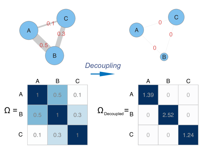
Figure 1: A simple example of our decoupling approach. $\mathbf{\Omega}$ and $\mathbf{\Omega}_{\text{Decoupled}}$ are the covariance matrices of the statistics of three studies A, B, and C before and after decoupling respectively. The thickness of the edges denotes the amount of correlation between the studies. After decoupling, the size of the nodes reflects the information that the studies contain in terms of the inverse variance.

Many traditional as well as recently proposed meta-analytic methods exist, but a majority of them cannot account for overlapping subjects (Table 1). Moreover, even if there exists a solution for overlapping subjects in a specific method such as the fixed effects model, the software one prefers may not support overlapping subjects. For example, widely used software METAL [18] and MANTEL [2] do not support overlapping subjects. We propose a general framework that allows different approaches to deal with overlapping subjects, which extends the Lin and Sullivan approach [17]. Through this paper, we will often use the term “correlation of studies” to refer to the correlation of statistics (typically z-scores) of studies in short. The intuition is that the more studies are correlated, the less information they contain with respect to the summary statistic of the meta-analysis. For example, if two studies are perfectly correlated ($r=1$), their combined information is not better than a single study’s information. In Figure 1, we have three studies A, B, and C whose statistics are correlated. For simplicity, their variances are set to 1.0. Our approach “decouples” the studies into independent studies that have the same information with respect to the summary statistic. The penalty for the decoupling is the increased variances. The variance of the study B has increased the most drastically (2.52), because its correlations to A and C were large (0.5 and 0.3). The size of the circles denotes the amount of information in terms of the inverse variance, showing that B has the smallest information. We can then use the decoupled studies in the downstream meta-analysis method. If the downstream method is the fixed effects model, our decoupling approach is equivalent to the optimal method of Lin and Sullivan [17] (See Methods).

2.2 False positive rate and power simulations

We perform simulations to examine the false positive rate and power of our decoupling approach. We suppose that ten different studies are combined in a meta-analysis to test a genotyped marker. We make an assumption that the studies are uniform in their sample sizes and the marker allele frequencies. We also assume that the sample sizes are sufficiently large. Under these assumptions, simulating genotype data is approximately equivalent to simulating the observed effect sizes directly from a normal distribution. For simplicity, we assume that the variances of effect sizes are uniformly 1.0. We use the significance threshold $\alpha=0.05$ for all simulations below.

We first simulate the null model in which the marker is not associated with a disease in all studies. We assume that the correlation $r_{ij}$ between study $i$ and $j$ is uniform for all study pairs $i\neq j$. This defines our covariance matrix $\mathbf{\Omega}$. Then we sample the vector of observed effect sizes $\hat{\mathbf{x}}$ from $N(0,\mathbf{\Omega})$ 10,000 times. We vary $r_{ij}$ from 0.0 to 0.9 and measure the false positive rates for different meta-analytic approaches.

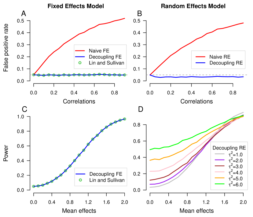
Figure 2: The false positive rate and power of different methods under the fixed and the random effects model. (A, B) We simulate studies assuming the null model of no associations. (C) We simulate studies assuming the alternative model based on the fixed effects model where the effect sizes are fixed across studies. We vary the magnitude of the fixed effect size. (D) We simulate studies assuming the alternative model based on the random effects model where the effect sizes vary across studies with an additional variance $\tau^{2}$. We vary both the magnitude of the mean effect size and the heterogeneity $\tau^{2}$.

In Figure 2A, we compare the false positive rate of the methods for the fixed effects model. The naive FE method refers to the traditional fixed effects model unaccounting for the correlations. The naive method shows dramatically inflated false positive rate as expected, since the correlations are ignored. The false positive rate becomes exacerbated as the unaccounted correlation increases, up to $0.52$ at $r_{ij}=0.9$. The decoupling FE refers to our decoupling approach applying FE after decoupling the studies. Both the decoupling FE and the Lin-Sullivan approach correctly control the false positive rate. The two methods yield the identical results, since they are equivalent (See Methods). The average false positive rate of the two methods over all correlation values $r_{ij}$ was identically 0.050.

In Figure 2B, we assess the false positive rate of the methods for the random effects model. The naive RE method refers to the Han and Eskin random effects model [8] unaccounting for the correlation. The naive method shows dramatically inflated false positive rate that increases with the correlation. The decoupling RE refers to our decoupling approach applying the Han and Eskin random effects model [8] after decoupling the studies. The decoupling RE correctly controls the false positive rate, with some conservative tendencies. The average false positive rate of the decoupling RE over all correlation values $r_{ij}$ was 0.034.

In Figure 2C, we simulate the alternative model assuming that the fixed effects model is the generative model. We fix the correlation to be $r_{ij}=0.20$. We sample $\hat{\mathbf{x}}$ from $N(\beta\mathbf{e},\mathbf{\Omega})$ where we vary the mean effect $\beta$ from 0.0 to 2.0. The decoupling FE shows power increase as the mean effect increases. The power is identical to the Lin-Sullivan approach, since the two methods are equivalent. Note that the naive FE method is not shown in the power comparison since its false positive rate is not properly controlled.

In Figure 2D, we simulate the alternative model assuming that the random effects model is the generative model. Again, we fix the correlation to be $r_{ij}=0.20$. We sample $\hat{\mathbf{x}}$ from $N(\beta\mathbf{e},\mathbf{\Omega}+\tau^{2}I)$ where we vary both $\beta$ and the heterogeneity $\tau^{2}$. The power of the decoupling RE is shown for different configurations of the models. We find that the power shows typical characteristics of the random effects model; the power increases as the mean effect increases and as the heterogeneity increases [8]. This shows that when we direct decoupled studies into the random effects model, the method has power to detect alternative models that the random effects model is designed for.

In summary, our simulations stress a few points; (1) The decoupling approach can be flexibly applied to both the fixed and the random effects models. (2) When applied to the fixed effects model, the decoupling approach shows equivalent results to the Lin-Sullivan approach. The method accurately controls the false positive rate and shows power to detect the alternative model. (3) When applied to the random effects model, the decoupling approach controls the false positive rate with conservative tendencies, while retaining the power to detect alternative models of the random effects model.

2.3 Applications to the Wellcome Trust Case Control Consortium data

We apply our decoupling approach to the Wellcome Trust Case Control Consortium (WTCCC) data. The WTCCC has performed genome-wide association studies of seven diseases (bipolar disorder, coronary artery disease, Crohn’s disease, hypertension, rheumatoid arthritis, type 1 diabetes, and type 2 diabetes, or BD, CAD, CD, HT, RA, T1D, and T2D in short). Using these data, we perform meta-analysis of three autoimmune diseases (CD, RA, and T1D). These data sets are a good example of overlapping subjects because all of the controls are shared between diseases. The WTCCC performed a combined analysis using the genotype data of these three diseases and reported four significant loci (See Supplementary Table 11 of Burton et al. [16]). We want to show the utility of our approach by reproducing the same results only using summary statistics without genotype data.

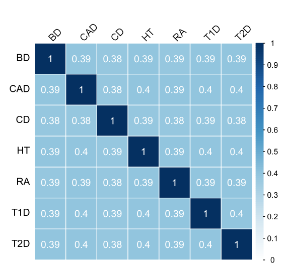
Figure 3: The correlation structure of the statistics of seven diseases in the WTCCC data. All seven diseases have approximately 2,000 cases and share 2,938 controls.

We first calculate the correlation matrix between the seven diseases using the Lin and Sullivan formula (See equation (4) in Methods). Figure 3 shows that the studies are positively correlated due to the shared control design. The correlations are at around $r=0.4$ at all pairs of the diseases. These uniform correlations reflects the unique study design that all controls are shared and the similar numbers of cases are collected in all diseases.

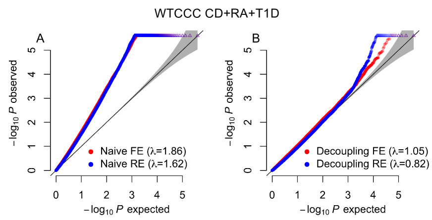
Figure 4: The qq-plots of a meta-analysis combining CD, RA, and T1D of the WTCCC data. The MHC region is excluded.

We perform the meta-analysis of three autoimmune diseases (CD, RA, and T1D) using the log odds ratios and their standard errors. We consider 397,450 SNPs that passed quality control for all three diseases and the minor allele frequency is greater than 1%. We first apply the naive fixed effects model (FE) and the random effects model (RE) which do not take into account the correlation structure. Figure 4A shows that the qq-plot is highly inflated for both the naive FE and the naive RE (the genomic control factors [19], $\lambda_{\text{FE}}=1.86$ and $\lambda_{\text{RE}}=1.62$, excluding the MHC region). Since the p-values are highly inflated, further downstream analyses using these naive approaches can be susceptible to false positives.

We then apply our decoupling approach to account for the correlation structure. We construct the decoupled studies and apply FE and RE. Figure 4B shows that the qq-plot is much better calibrated ($\lambda_{\text{FE}}=1.05$ and $\lambda_{\text{RE}}=0.82$). Both the decoupling FE and RE approaches identified the four loci as significant ($P<1.2\times 10^{-7}$, Bonferroni corrected for $397,450$ tests) that were reported in the combined analysis of the WTCCC study [16] (Table 2). This shows that our approach was able to reproduce the previously reported results only using the summary statistics.

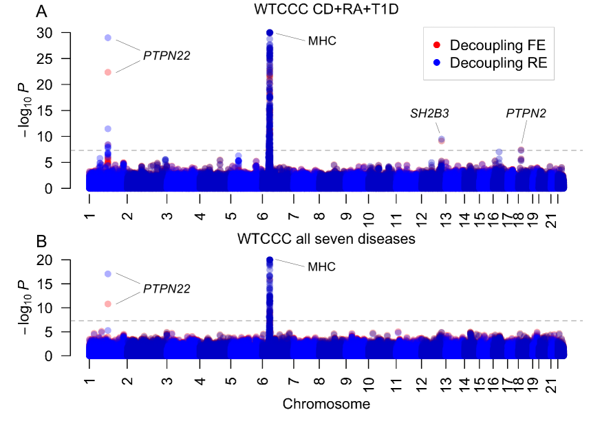
Figure 5: The Manhattan plots of meta-analyses combining a set of diseases of the WTCCC data. (A) We combine CD, RA, and T1D. (B) We combine all seven diseases.

Moreover, our decoupling approach has an advantage over the combined analysis [16]. Since our approach can utilize both FE and RE, one can have good power to detect both the homogeneous and the heterogeneous effects [8]. By contrast, the combined analysis can be thought of as similar to FE and may not have good power to detect heterogeneous effects. In the Manhattan plot (Figure 5), the notable peaks are the PTPN22 gene in the chromosome 1 and the major histocompatibility complex (MHC) region in the chromosome 6. Both loci are known to play an important role in autoimmune diseases [3, 4]. At both loci, the decoupling RE yields more significant p-values than the decoupling FE (PTPN22: $P_{\text{FE}}=5\times 10^{-23}$ and $P_{\text{RE}}=1\times 10^{-29}$, MHC: $P_{\text{FE}}=5\times 10^{-80}$ and $P_{\text{RE}}=8\times 10^{-181}$). This is because of the heterogeneous nature of these two loci that they are strongly associated to RA and T1D but weakly to CD (Table 2). This shows that our decoupling approach can allow one to flexibly apply different meta-analytic approaches that are optimized for different situations.

Finally, we examine the robustness of our decoupling approach by adding the other four diseases as noisy data into the meta-analysis. Figure 5B shows that when we meta-analyze all seven diseases, the absolute magnitudes of the significance of PTPN22 and MHC loci are reduced, but they are still significant for both the decoupling FE and the decoupling RE. Moreover, the relative significance gain of the decoupling RE compared to the decoupling FE is still largely pronounced (PTPN22: $P_{\text{FE}}=1\times 10^{-11}$ and $P_{\text{RE}}=9\times 10^{-18}$, MHC: $P_{\text{FE}}=1\times 10^{-28}$ and $P_{\text{RE}}=1\times 10^{-89}$).

3 Materials and Methods

3.1 Meta-analytic methods

We first briefly describe some of the existing meta-analytic methods.

Fixed effects model

The fixed effects model approach (FE) assumes that the magnitude of the effect size is fixed across the studies [5, 6]. The two widely used methods are the inverse-variance-weighted effect size method [1] and the weighted sum of z-scores method [2]. Since the two methods are approximately equivalent [8], we only describe the inverse-variance-weighted effect size method. Let $X_{1},...,X_{N}$ be the effect size estimates in $N$ independent studies such as the log odds ratios or regression coefficients. Let $\textrm{SE}(X_{i})$ be the standard error of $X_{i}$ and let $V_{i}=\textrm{SE}(X_{i})^{2}$. Let $W_{i}=V_{i}^{-1}$ be the inverse variance. The inverse-variance-weighted summary effect size is

$$X_{\text{FE}}=\frac{\sum W_{i}X_{i}}{\sum W_{i}}\;.$$ (1)

The variance of $X_{\text{FE}}$ is

$$V_{\text{FE}}=\frac{1}{\sum W_{i}}\;.$$ (2)

Since the standard error of $X_{\text{FE}}$ is $\textrm{SE}(X_{\text{FE}})=\sqrt{\sum W_{i}}^{-1}$, we can construct a summary z-score

$$Z_{\text{FE}}=\frac{X_{\text{FE}}}{\textrm{SE}(X_{\text{FE}})}=\frac{\sum W_{i}X_{i}}{\sqrt{\sum W_{i}}}$$

that follows ${N}(0,1)$ under the null hypothesis of no associations. The p-value is calculated

$$p_{\text{FE}}=2\Phi\big{(}-|Z_{\text{FE}}|\big{)}$$

where $\Phi$ is the cumulative density function of the standard normal distribution.

Random effects model

In the random effects (RE) model, it is assumed that the effect size varies among studies, a phenomenon called heterogeneity. RE assumes that the effect size follows the probability distribution with variance $\tau^{2}$. There are several approaches to estimate the variance $\tau^{2}$, the most common one being the moment-based estimator of DerSimonian and Laird [7]. Given the estimate ($\hat{\tau}^{2}$) of $\tau^{2}$, the summary effect size estimate is calculated as

$$X_{\text{RE}}=\frac{\sum\left(W^{-1}_{i}+{\hat{\tau}}^{2}\right)^{-1}X_{i}}{\sum\left(W^{-1}_{i}+{\hat{\tau}}^{2}\right)^{-1}}$$

The standard error of $X_{\text{RE}}$ is $\textrm{SE}(X_{\text{RE}})=\sqrt{\sum\left(W^{-1}_{i}+{\hat{\tau}}^{2}\right)^{-1}}^{-1}$. In the traditional RE approach, one constructs a z-score statistic

$$Z_{\text{RE}}=\frac{X_{\text{RE}}}{\textrm{SE}(X_{\text{RE}})}$$

and the p-value is computed as $p_{\text{RE}}=2\Phi\big{(}-|Z_{\it RE}|\big{)}$. Recently, Han and Eskin found that the traditional RE is conservative and rarely achieves higher power than the fixed effects model [8]. This is because of the conservatie null hypothesis of the traditional RE that implicitly assumes heterogeneity under the null. They proposed a new random effects model that corrects for this problem, and the test statistic is

$$S_{\text{NewRE}}=\sum\text{log}\left(\frac{V_{i}}{V_{i}+\hat{\tau}^{2}}\right)+\sum\frac{X_{i}^{2}}{V_{i}}-\sum\frac{\left(X_{i}-\hat{\mu}\right)^{2}}{V_{i}+\hat{\tau}^{2}}$$ (3)

where $\hat{\mu}$ and $\hat{\tau}^{2}$ are the maximum likelihood estimations of mean and variance of the effect size, respectively, which can be found by an iterative procedure. The statistic follows a half and half mixture of $\chi^{2}_{(0)}$ and $\chi^{2}_{(1)}$ under the null [20]. The p-value can be calculated by using the asymptotic distribution or using a pre-constructed p-value table for a more accurate calculation accounting for the small number of observations [8].

P-value-based approaches

There exist meta-analytic approaches combining p-values instead of effect sizes, the most traditional one being the Fisher’s method [9]. The Fisher’s method combines the p-values $p_{1},...,p_{N}$ by constructing a statistic

$$S_{\text{Fisher}}=-2\sum_{i=1}^{N}\log(p_{i})$$

which follows $\chi^{2}_{(2N)}$ under the null. The p-value-based approaches have advantages that it can be used even when one does not have information about the direction of effects. A recently proposed p-value-based approach by Zaykin and Kozbur can take into account overlapping subjects [10].

Subset approaches

Subset approaches have similarities to the fixed effects model, but the difference is that one assumes that the effects can exist in only a subset of the studies. Han and Eskin computes a statistic called “m-value”, a posterior probability that the effect is present in a study [12]. The m-values are incorporated in the weighted z-score FE approach to upweight studies with high m-values. The p-value is assessed using the importance sampling. Bhattacharjee et al. [11] proposed an approach that computes FE statistics using all possible subsets of studies in a meta-analysis and uses the maximum statistic. The method expedites the enumeration of all possible $2^{N}-1$ possible subsets of $N$ studies by using a novel statistical technique. This method can account for overlapping subjects.

Bayesian approaches

Morris proposed a Bayesian approach optimized for the trans-ethnic meta-analysis [14]. This method utilizes the Markov Chain Monte Carlo (MCMC) procedure to navigate through possible disease models. In his MCMC, closely related populations have higher chance to have similar effect sizes to increase the statistical power to detect heterogeneity caused by the population spectrum. Wen [13] proposed a new method taking into account heterogeneity in the data using the hierarchical model in the Bayesian framework. Wen [15] recently extended this method to a multi-way table modeling, which can account for the correlation structure between studies or the overlapping subjects.

3.2 Lin and Sullivan approach

Lin and Sullivan proposed a systematic approach for dealing with overlapping subjects for the fixed effects model [17]. The first step of their approach is to analytically calculate the correlation of the statistics $X_{1},...,X_{N}$ caused by the overlapping subjects. Let $\mathbf{x}$ be the vector of effect size estimates $\mathbf{x}=(X_{1},...,X_{N})$ and let

$$\mathbf{C}=\big{[}r_{ij}\big{]}_{N\times N}$$

be the correlation matrix of $X$ where $r_{ij}$ denotes the the correlation between $X_{i}$ and $X_{j}$. $r_{ij}$ is analytically approximated with the formula

$$r_{ij}\approx\left(n_{ij0}\sqrt{\frac{n_{i1}n_{j1}}{n_{i0}n_{j0}}}+n_{ij1}\sqrt{\frac{n_{i0}n_{j0}}{n_{i1}n_{j1}}}\right)\Big{/}\sqrt{n_{i}n_{j}}$$ (4)

$n_{i1}$, $n_{i0}$, and $n_{i}$ (or $n_{j1}$, $n_{j0}$, and $n_{j}$) are the number of cases, the number of controls, and the total number of subjects in the $i$th (or $j$th) study, respectively. $n_{ij1}$ and $n_{ij0}$ are the numbers of cases and controls that overlap between the $i$th and $j$th studies. See Bhattacharjee et al. [11] for an extended formula for the situation that some cases in one study are controls in other studies. Given the correlation matrix $\mathbf{C}$, it is straightforward to calculate the covariance matrix $\mathbf{\Omega}$.

The second step of the Lin and Sullivan approach is to optimally take into account $\mathbf{\Omega}$ in the testing. The optimal fixed effects model meta-analysis statistic is

$$X_{\text{Lin}}=\frac{\mathbf{e}^{T}\mathbf{\Omega}^{-1}\mathbf{x}}{\mathbf{e}^{T}\mathbf{\Omega}^{-1}\mathbf{e}}$$ (5)

where $\mathbf{e}$ is the vector of ones ($\mathbf{e}=(1,...,1)$). The formal proof for the optimality of this statistic is shown in [21] and [22]. We also present a simple reasoning for deriving this statistic in Supplementary Materials. The variance of the statistic is given

$$\mathrm{Var}\left(X_{\text{Lin}}\right)=\frac{1}{\mathbf{e}^{T}\mathbf{\Omega}^{-1}\mathbf{e}}$$ (6)

The z-score $X_{\text{Lin}}/\sqrt{\mathrm{Var}\left(X_{\text{Lin}}\right)}$ is calculated to obtain the p-value. Note that in a special case that $X_{1},...,X_{N}$ are independent ($\mathbf{\Omega}$ is a diagonal matrix), $X_{\text{Lin}}$ equals to $X_{\text{FE}}$ and $\mathrm{Var}\left(X_{\text{Lin}}\right)$ equals to $\mathrm{Var}\left(X_{\text{FE}}\right)$.

3.3 Decoupling approach

We extend the Lin and Sullivan approach to a general framework that can be applied to a wide range of meta-analytic methods. Our approach “uncorrelates” or “decouples” correlated studies into independent studies whose standard errors are updated to account for the decoupling. Suppose that we are given the effect sizes $\mathbf{x}$, the standard errors of them $\mathbf{s}$, and the correlation matrix $\mathbf{C}$ computed by the formula (4). The decoupling procedure is the following.

1. Keep the original $\mathbf{x}$.
   $\mathbf{x}_{\text{Decoupled}}\leftarrow\mathbf{x}$

2. Compute the covariance matrix of $\mathbf{x}$.
   $\mathbf{\Omega}\leftarrow Diag(\mathbf{s})\cdot\mathbf{C}\cdot Diag(\mathbf{s})$

3. Compute the decoupled covariance matrix.
   $\mathbf{\Omega}_{\text{Decoupled}}\leftarrow Diag(\mathbf{e}^{T}\mathbf{\Omega}^{-1})^{-1}$

4. Update the standard errors.
   $\mathbf{s}_{\text{Decoupled}}[i]\leftarrow\sqrt{\mathbf{\Omega}_{\text{Decoupled}}[i,i]}$ for each $i=1,...,N$

5. Use $\mathbf{x}_{\text{Decoupled}}$ and $\mathbf{s}_{\text{Decoupled}}$ in the downstream meta-analysis.

$Diag(\mathbf{s})$ denotes a diagonal matrix whose diagonals are $\mathbf{s}$. The brakets [ ] denote the index of an element of a vector or a matrix. In Supplementary Materials, we present a simple R code performing this procedure.

We give a simple working example of this procedure. Suppose that we have two effect sizes $X_{1}$ and $X_{2}$. For simplicity, let their variances be 1.0. Under the fixed effects model, the best summary estimate of effect size will be $(X_{1}+X_{2})/2$ and its variance will be $1.0/2=0.5$, which will be the correct variance if the two studies are independent ($r_{12}=0$). Now consider the case that $X_{1}$ and $X_{2}$ are highly correlated ($r_{12}=0.99$). Intuitively, since they are highly correlated, the information they contain is not much better than the information a single study contains. The decoupling formula gives us the new variance of each study increased to $1.99$. When we plug the new variances into the fixed effects model, the variance of the summary effect size will be $1.99/2=0.995\approx 1.0$ showing that as expected, the uncertainty in the final estimate is approximately the same as the uncertainty that we would obtain with a single study.

Observation 1.

Using the decoupled studies in the fixed effects model is equivalent to the Lin and Sullivan approach.

Proof.

Given a covariance matrix $\mathbf{\Omega}$, our decoupling approach will calculate the updated standard errors $\mathbf{s}_{\text{Decoupled}}$ by calculating $\mathbf{\Omega}_{\text{Decoupled}}$. Since $\mathbf{\Omega}_{\text{Decoupled}}$ is a diagonal matrix, the following relationship holds

$$\mathbf{\Omega}_{\text{Decoupled}}=Diag(\mathbf{s}_{\text{Decoupled}})\cdot Diag(\mathbf{s}_{\text{Decoupled}})$$

On the other hand, given an effect size vector $\mathbf{x}$ and standard errors $\mathbf{s}$, the standard fixed effects model formulae in equation (1) and (2) can be written

$$X_{\text{FE}}=\frac{\mathbf{e}^{T}\mathbf{V}^{-1}\mathbf{x}}{\mathbf{e}^{T}\mathbf{V}^{-1}\mathbf{e}}$$

and

$$V_{\text{FE}}=\frac{1}{\mathbf{e}^{T}\mathbf{V}^{-1}\mathbf{e}}$$

where $\mathbf{V}=Diag(\mathbf{s})\cdot Diag(\mathbf{s})$. If we plug $\mathbf{s}_{\text{Decoupled}}$ into this formula,

$$X_{\text{FE}} =\frac{\mathbf{e}^{T}\mathbf{V}^{-1}\mathbf{x}}{\mathbf{e}^{T}\mathbf{V}^{-1}\mathbf{e}}$$

$$=\frac{\mathbf{e}^{T}(Diag(\mathbf{s}_{\text{Decoupled}})\cdot Diag(\mathbf{s}_{\text{Decoupled}}))^{-1}\mathbf{x}}{\mathbf{e}^{T}(Diag(\mathbf{s}_{\text{Decoupled}})\cdot Diag(\mathbf{s}_{\text{Decoupled}}))^{-1}\mathbf{e}}$$

$$=\frac{\mathbf{e}^{T}\mathbf{\Omega}_{\text{Decoupled}}^{-1}\mathbf{x}}{\mathbf{e}^{T}\mathbf{\Omega}_{\text{Decoupled}}^{-1}\mathbf{e}}$$

$$=\frac{\mathbf{e}^{T}Diag(\mathbf{e}^{T}\mathbf{\Omega}^{-1})\mathbf{x}}{\mathbf{e}^{T}Diag(\mathbf{e}^{T}\mathbf{\Omega}^{-1})\mathbf{e}}$$

$$=\frac{\mathbf{e}^{T}\mathbf{\Omega}^{-1}\mathbf{x}}{\mathbf{e}^{T}\mathbf{\Omega}^{-1}\mathbf{e}}$$

$$=X_{\text{Lin}}$$

where $X_{\text{Lin}}$ is in equation (5). Similarly, we can show that $V_{\text{FE}}$ equals to $V_{\text{Lin}}$ in equation (6). Therefore, applying our decoupling approach to the fixed effects model is equivalent to the Lin an Sullivan approach [17].

∎

4 Discussions

We proposed a general framework for dealing with overlapping subjects in a meta-analysis. The core idea is to “decouple” the correlated studies into independent studies and use them in the downstream meta-analysis. Our approach can flexibly allow many meta-analytic methods, such as the random effects model, to account for overlapping subjects. The simulations and the applications to the WTCCC data support the utilities of our approach.

Since our approach involves only the data-side change rather than the method-side change, one advantage is that one can continue to use preferred software in the existing analysis pipeline which may not support overlapping subjects. This can be important in practice, since it can be inconvenient to change a pipeline. For example, one may have been using METAL [18] or MANTEL [2] for automatically detecting strand inconsistencies between studies and for automatically applying the genomic control [19]. Given new data with overlapping subjects, one does not need to switch to different software supporting overlapping subjects but can simply update the standard errors using our approach and continue to use the existing pipeline.

In this paper, we primarily focused on dealing with overlapping subjects, but our decoupling approach can be applied to any contexts of meta-analysis where the inputs are correlated. For example, in an eQTL study, multiple tissues can be analyzed together in a meta-analysis framework [23]. Since tissues of the same individual are correlated, this results in a meta-analytic problem where the inputs are correlated. In such cases, our decoupling approach with FE and RE methods can be applied to detect both tissue-specific and shared eQTLs [23].

The limitation of our approach is that the optimality is guaranteed only under the fixed effects model. For example, our simulations show that our approach has some conservative tendencies under the random effects model, indicating that our approach may not be optimal, although we showed that it works well in the simulations and the WTCCC data. Optimal solutions to account for correlated inputs for each different meta-analytic method will be an interesting topic for further research.

We note that one should be careful in interpreting data based on the decoupled studies. For example, the heterogeneity testing is highly conservative when using decoupled studies and may not well detect true heterogeneity. Unfortunately, there is no good alternative to the Cochran’s Q test and the $I^{2}$ estimate that can take into account correlated inputs yet. Developing such methods will also be an interesting future research area.

5 Tables and Figures

Category	Method	Supports overlapping subjects
Fixed effects model	Traditional FE [5, 6]	No
	Lin and Sullivan [17]	Yes
Random effects model	Traditional RE [7]	No
	Han and Eskin RE [8]	No
P-value-based approaches	Fisher’s approach [9]	No
	Zaykin and Kozbur [10]	Yes
Subset approaches	Bhattacharjee et al. [11]	Yes
	Binary Effects Model [12]	No
Bayesian approaches	Hierarchical Bayesian approach [13]	No
	Trans-ethnic approach [14]	No
	Multi-way table approach [15]	Yes

Table 1: Different meta-analytic methods and their support for overlapping subjects.

			Single disease P-values				Meta-analysis P-values
Chr.	RSID	Position	CD	RA	T1D		Decouple-FE	Decouple-RE	Genes
1	rs6679677	114015850	0.0372	$4.46\times 10^{-16}$	$2.20\times 10^{-17}$		$4.48\times 10^{-23}$	$1.00\times 10^{-29}$	PTPN22
6	rs9273363	32734250	0.225	$5.18\times 10^{-07}$	$8.14\times 10^{-180}$		$5.02\times 10^{-80}$	$7.72\times 10^{-181}$	HLA genes
12	rs17696736	110949538	0.0189	0.0281	$1.98\times 10^{-09}$		$7.72\times 10^{-10}$	$3.40\times 10^{-10}$	SH2B3
18	rs2542151	12769947	$3.66\times 10^{-05}$	0.0841	0.000297		$3.74\times 10^{-08}$	$5.16\times 10^{-08}$	PTPN2

Table 2: Association results of a meta-analysis combining CD, RA, and T1D of the WTCCC data. The four loci reported in the WTCCC combined analysis [16] are presented. The curated list of candidate genes for each loci are obtained from the ImmunoBase web site (www.ImmunoBase.org).

6 Supplementary Materials

6.1 Optimality of Lin and Sullivan approach

We present a simple reasoning to derive and show the optimality of the Lin and Sullivan statistic in equation (5). Note that the formal proof of the optimality is shown in [22] and [21], and there can be many other proofs. The equation (5) is

$$X_{\text{Lin}}=\frac{\mathbf{e}^{T}\mathbf{\Omega}^{-1}\mathbf{x}}{\mathbf{e}^{T}\mathbf{\Omega}^{-1}\mathbf{e}}$$

where the notations are described in Methods. One simple way to derive this statistic is to translate the problem of finding a summary statistic to a linear regression framework. Consider that $\mathbf{x}$ is the dependent variables whose variance is $\mathbf{\Omega}$. Then finding the best summary statistic is equivalent to finding the best mean or the intercept $\beta$. Thus, we have a regression model including only the intercept term

$$\mathbf{x}=\beta\mathbf{e}+\epsilon$$

where $\mathrm{Var}\left(\epsilon\right)=\mathbf{\Omega}$. By the standard generalized least square formula, the optimal estimate of $\beta$ will be

$$\hat{\beta}=(\mathbf{e}^{T}\mathbf{\Omega}^{-1}\mathbf{e})^{-1}\mathbf{e}^{T}\mathbf{\Omega}^{-1}\mathbf{x}$$

Since $\mathbf{e}^{T}\mathbf{\Omega}^{-1}\mathbf{e}$ is a scalar, this form is equivalent to $X_{\text{Lin}}$.

6.2 R code performing decoupling approach

## Decoupling approach.
## Input:
##   s is the standard errors (possibly with NA)
##   C is the correlation matrix
##   (or one can specify C.inv (inverse of C) for speed-up)
## Output:
##   updated standard errors after decoupling
decoupling <- function(s, C, C.inv=NULL) {
  i <- !is.na(s)
  if (is.null(C.inv)) {
    Omega.inv <- solve(diag(s[i]) %*% C[i,i] %*% diag(s[i]))
  } else {
    Omega.inv <- diag(1/s[i]) %*% C.inv[i,i] %*% diag(1/s[i])
  }
  s.new <- sqrt(1/rowSums(Omega.inv))
  s[i] <- s.new
  s
}

References

- 1. Joseph. L. Fleiss. The statistical basis of meta-analysis. Stat Methods Med Res, 2(2):121–145, 1993.
- 2. Paul I. W. de Bakker, Manuel A. R. Ferreira, Xiaoming Jia, Benjamin M. Neale, Soumya Raychaudhuri, and Benjamin F. Voight. Practical aspects of imputation-driven meta-analysis of genome-wide association studies. Hum Mol Genet, 17(R2):R122–R128, October 2008.
- 3. Steve Eyre, John Bowes, Dorothée Diogo, Annette Lee, Anne Barton, Paul Martin, Alexandra Zhernakova, Eli Stahl, Sebastien Viatte, Kate McAllister, Christopher I. Amos, Leonid Padyukov, Rene E. M. Toes, Tom W. J. Huizinga, Cisca Wijmenga, Gosia Trynka, Lude Franke, Harm-Jan Westra, Lars Alfredsson, Xinli Hu, Cynthia Sandor, Paul I. W. de Bakker, Sonia Davila, Chiea Chuen Khor, Khai Koon Heng, Robert Andrews, Sarah Edkins, Sarah E Hunt, Cordelia Langford, Deborah Symmons, Pat Concannon, Suna Onengut-Gumuscu, Stephen S. Rich, Panos Deloukas, Miguel A Gonzalez-Gay, Luis Rodriguez-Rodriguez, Lisbeth Ärlsetig, Javier Martin, Solbritt Rantapää-Dahlqvist, Robert M. Plenge, Soumya Raychaudhuri, Lars Klareskog, Peter K. Gregersen, and Jane Worthington. High-density genetic mapping identifies new susceptibility loci for rheumatoid arthritis. Nat Genet, 44(12):1336–1340, November 2012.
- 4. Luke L Jostins, Stephan S Ripke, Rinse K RK Weersma, Richard H RH Duerr, Dermot P DP McGovern, Ken Y KY Hui, James C JC Lee, L Philip LP Schumm, Yashoda Y Sharma, Carl A CA Anderson, Jonah J Essers, Mitja M Mitrovic, Kaida K Ning, Isabelle I Cleynen, Emilie E Theatre, Sarah L SL Spain, Soumya S Raychaudhuri, Philippe P Goyette, Zhi Z Wei, Clara C Abraham, Jean-Paul JP Achkar, Tariq T Ahmad, Leila L Amininejad, Ashwin N AN Ananthakrishnan, Vibeke V Andersen, Jane M JM Andrews, Leonard L Baidoo, Tobias T Balschun, Peter A PA Bampton, Alain A Bitton, Gabrielle G Boucher, Stephan S Brand, Carsten C Büning, Ariella A Cohain, Sven S Cichon, Mauro M D’Amato, Dirk D De Jong, Kathy L KL Devaney, Marla M Dubinsky, Cathryn C Edwards, David D Ellinghaus, Lynnette R LR Ferguson, Denis D Franchimont, Karin K Fransen, Richard R Gearry, Michel M Georges, Christian C Gieger, Jürgen J Glas, Talin T Haritunians, Ailsa A Hart, Chris C Hawkey, Matija M Hedl, Xinli X Hu, Tom H TH Karlsen, Limas L Kupcinskas, Subra S Kugathasan, Anna A Latiano, Debby D Laukens, Ian C IC Lawrance, Charlie W CW Lees, Edouard E Louis, Gillian G Mahy, John J Mansfield, Angharad R AR Morgan, Craig C Mowat, William W Newman, Orazio O Palmieri, Cyriel Y CY Ponsioen, Uros U Potocnik, Natalie J NJ Prescott, Miguel M Regueiro, Jerome I JI Rotter, Richard K RK Russell, Jeremy D JD Sanderson, Miquel M Sans, Jack J Satsangi, Stefan S Schreiber, Lisa A LA Simms, Jurgita J Sventoraityte, Stephan R SR Targan, Kent D KD Taylor, Mark M Tremelling, Hein W HW Verspaget, Martine M De Vos, Cisca C Wijmenga, David C DC Wilson, Juliane J Winkelmann, Ramnik J RJ Xavier, Sebastian S Zeissig, Bin B Zhang, Clarence K CK Zhang, Hongyu H Zhao, Mark S MS Silverberg, Vito V Annese, Hakon H Hakonarson, Steven R SR Brant, Graham G Radford-Smith, Christopher G CG Mathew, John D JD Rioux, Eric E EE Schadt, Mark J MJ Daly, Andre A Franke, Miles M Parkes, Severine S Vermeire, Jeffrey C JC Barrett, and Judy H JH Cho. Host-microbe interactions have shaped the genetic architecture of inflammatory bowel disease. Nature, 491(7422):119–124, November 2012.
- 5. William G. Cochran. The Combination of Estimates from Different Experiments. Biometrics, 10:101–129, March 1954.
- 6. Nathan Mantel and William Haenszel. Statistical aspects of the analysis of data from retrospective studies of disease. J Natl Cancer Inst, 22(4):719–748, April 1959.
- 7. R. DerSimonian and N. Laird. Meta-analysis in clinical trials. Controlled clinical trials, 7(3):177–188, September 1986.
- 8. Buhm Han and Eleazar Eskin. Random-effects model aimed at discovering associations in meta-analysis of genome-wide association studies. The American Journal of Human Genetics, 88(5):586–598, May 2011.
- 9. R. A. Fisher. Statistical Methods for Research Workers. 13th Ed. Oliver & Boyd, 1967.
- 10. Dmitri V Zaykin and Damian O Kozbur. P-value based analysis for shared controls design in genome-wide association studies. Genet Epidemiol, 34(7):725–738, October 2010.
- 11. Samsiddhi Bhattacharjee, Preetha Rajaraman, Kevin B. Jacobs, William A Wheeler, Beatrice S Melin, Patricia Hartge, Meredith Yeager, Charles C Chung, Stephen J. Chanock, Nilanjan Chatterjee, and GliomaScan Consortium7. A Subset-Based Approach Improves Power and Interpretation for the Combined Analysis of Genetic Association Studies of Heterogeneous Traits. The American Journal of Human Genetics, 90(5):821–835, May 2012.
- 12. Buhm Han and Eleazar Eskin. Interpreting meta-analyses of genome-wide association studies. PLoS Genet, 8(3):e1002555, March 2012.
- 13. Xiaoquan Wen and Matthew Stephens. Bayesian Methods for Genetic Association Analysis with Heterogeneous Subgroups: from Meta-Analyses to Gene-Environment Interactions. arXiv.org, arXiv:1111.1210, November 2011.
- 14. Andrew P. Morris. Transethnic meta-analysis of genomewide association studies. Genet Epidemiol, 35(8):809–822, November 2011.
- 15. Xiaoquan Wen. Bayesian Analysis of Multiway Tables in Association Studies: A Model Comparison Approach. arXiv.org, arXiv:1208.4621, August 2012.
- 16. Paul R Burton, David G. Clayton, Lon R. Cardon, Nick Craddock, Panos Deloukas, Audrey Duncanson, Dominic P Kwiatkowski, Mark I. McCarthy, Willem H. Ouwehand, Nilesh J. Samani, John A. Todd, Peter Donnelly, Jeffrey C. Barrett, Paul R Burton, Dan Davison, Peter Donnelly, Doug Easton, David Evans, Hin-Tak Leung, Jonathan L. Marchini, Andrew P. Morris, Chris C A Spencer, Martin D Tobin, Lon R. Cardon, David G. Clayton, Antony P Attwood, James P Boorman, Barbara Cant, Ursula Everson, Judith M Hussey, Jennifer D Jolley, Alexandra S Knight, Kerstin Koch, Elizabeth Meech, Sarah Nutland, Christopher V Prowse, Helen E Stevens, Niall C Taylor, Graham R Walters, Neil M. Walker, Nicholas A Watkins, Thilo Winzer, John A. Todd, Willem H. Ouwehand, Richard W Jones, Wendy L. McArdle, Susan M. Ring, David P. Strachan, Marcus Pembrey, Gerome Breen, David St Clair, Sian Caesar, Katherine Gordon-Smith, Lisa Jones, Christine Fraser, Elaine K Green, Detelina Grozeva, Marian L Hamshere, Peter A Holmans, Ian R Jones, George Kirov, Valentina Moskvina, Ivan Nikolov, Michael C O’Donovan, Michael J Owen, Nick Craddock, David A Collier, Amanda Elkin, Anne Farmer, Richard Williamson, Peter McGuffin, Allan H Young, I Nicol Ferrier, Stephen G Ball, Anthony J Balmforth, Jennifer H Barrett, D Timothy Bishop, Mark M Iles, Azhar Maqbool, Nadira Yuldasheva, Alistair S. Hall, Peter S Braund, Paul R Burton, Richard J Dixon, Massimo Mangino, Suzanne Stevens, Martin D Tobin, John R Thompson, Nilesh J. Samani, Francesca Bredin, Mark Tremelling, Miles Parkes, Hazel Drummond, Charles W Lees, Elaine R Nimmo, Jack Satsangi, Sheila A Fisher, Alastair Forbes, Cathryn M Lewis, Clive M Onnie, Natalie J. Prescott, Jeremy Sanderson, Christopher G. Mathew, Jamie Barbour, M Khalid Mohiuddin, Catherine E Todhunter, John C. Mansfield, Tariq Ahmad, Fraser R Cummings, Derek P Jewell, John Webster, Morris J Brown, David G. Clayton, G. Mark Lathrop, John Connell, Anna Dominiczak, Nilesh J. Samani, Carolina A Braga Marcano, Beverley Burke, Richard Dobson, Johannie Gungadoo, Kate L Lee, Patricia B. Munroe, Stephen J Newhouse, Abiodun Onipinla, Chris Wallace, Mingzhan Xue, Mark Caulfield, Martin Farrall, Anne Barton, , The Biologics in RA Genetics Genomics BRAGGS, Ian N Bruce, Hannah Donovan, Steve Eyre, Paul D Gilbert, Samantha L Hider, Anne M Hinks, Sally L John, Catherine Potter, Alan J Silman, Deborah P M Symmons, Wendy Thomson, Jane Worthington, David G. Clayton, David B Dunger, Sarah Nutland, Helen E Stevens, Neil M. Walker, Barry Widmer, John A. Todd, Timothy M. Frayling, Rachel M. Freathy, Hana Lango, John R. B. Perry, Beverley M. Shields, Michael N. Weedon, Andrew T. Hattersley, Graham A. Hitman, Mark Walker, Kate S Elliott, Christopher J. Groves, Cecilia M. Lindgren, Nigel W. Rayner, Nicholas J. Timpson, Eleftheria Zeggini, Mark I. McCarthy, Melanie Newport, Giorgio Sirugo, Emily Lyons, Fredrik Vannberg, Adrian V S Hill, Linda A Bradbury, Claire Farrar, Jennifer J Pointon, Paul Wordsworth, Matthew A Brown, Jayne A Franklyn, Joanne M Heward, Matthew J Simmonds, Stephen C L Gough, Sheila Seal, Breast Cancer Susceptibility Collaboration UK, Michael R Stratton, Nazneen Rahman, Maria Ban, An Goris, Stephen J Sawcer, Alastair Compston, David Conway, Muminatou Jallow, Melanie Newport, Giorgio Sirugo, Kirk A Rockett, Dominic P Kwiatkowski, Suzannah J. Bumpstead, Amy Chaney, Kate Downes, Mohammed J. R. Ghori, Rhian Gwilliam, Sarah E Hunt, Michael Inouye, Andrew Keniry, Emma King, Ralph McGinnis, Simon Potter, Rathi Ravindrarajah, Pamela Whittaker, Claire Widden, David Withers, Panos Deloukas, Hin-Tak Leung, Sarah Nutland, Helen E Stevens, Neil M. Walker, John A. Todd, Doug Easton, David G. Clayton, Paul R Burton, Martin D Tobin, Jeffrey C. Barrett, David Evans, Andrew P. Morris, Lon R. Cardon, Niall J Cardin, Dan Davison, and Teresa… Ferreira. Genome-wide association study of 14,000 cases of seven common diseases and 3,000 shared controls. Nature, 447(7145):661–678, June 2007.
- 17. Dan-Yu Lin and Patrick F Sullivan. Meta-Analysis of Genome-wide Association Studies with Overlapping Subjects. The American Journal of Human Genetics, 85(6):862–872, December 2009.
- 18. Goncalo Abecasis. Metal - meta analysis helper (http://www.sph.umich.edu/csg/abecasis/metal).
- 19. B. Devlin and N Risch. A comparison of linkage disequilibrium measures for fine-scale mapping. Genomics, 29(2):311–322, September 1995.
- 20. S. G. Self and K. Y. Liang. Asymptotic properties of maximum likelihood estimators and likelihood ratio tests under nonstandard conditions. Journal of the American Statistical Association, 82(398):605–610, June 1987.
- 21. L J Wei, D Y Lin, and L Weissfeld. Regression Analysis of Multivariate Incomplete Failure Time Data by Modeling Marginal Distributions. Journal of the American Statistical Association, 84(408):1065–1073, December 1989.
- 22. L J Wei and Wayne E Johnson. Combining Dependent Tests with Incomplete Repeated Measurements. Biometrika, 72(2):359–364, 1985.
- 23. Jae-Hoon Sul, Buhm Han, Chun Ye, Ted Choi, and Eleazar Eskin. Effectively identifying eqtls from multiple tissues by combining mixed model and meta-analytic approaches. PLoS Genet, In Press, 2013.