BFKL Pomeron: modeling confinement

Abstract:

In this paper we introduce the confinement into the kernel of the BFKL equation, assuming that the sizes of produced dipoles cannot be large. The goal of this paper is to find how this assumption, which leads to a correct exponential decrease of the amplitude at large impact parameters, affects the main properties of the BFKL Pomeron. We solve the equations for total cross section and $\langle|b^{2}|\rangle$ numerically and developed some methods of analytical solutions. The main result is that the modified BFKL Pomeron has the same intercept and $\alpha^{\prime}_{I\!\!P}=0$ as the BFKL Pomeron. It gives us a hope that the unknown confinement will change only slightly the equations of the CGC/saturation approach.

1 Introduction

The large impact parameter dependence of the scattering amplitude has been the principle but still unsolved problem in the CGC/saturation approach for the past decade. It was shown in Refs.[1, 2, 3, 4] that CGC/saturation approach[5, 6, 7, 8] that leads to the partial amplitude smaller than unity and satisfies the unitarity constraints, generates the radius of interaction that increases as a power of energy in explicit contradiction to the Froissart theorem[9]. It stems from large $b$ behaviour of the BFKL Pomeron[11, 10] which has the form: $A\left(b\gg 1/Q_{s}\right)\,\,\propto\,\,s^{\Delta}/b^{2}$. Amplitude $A\left(b\gg 1/Q_{s}\right)$ becomes of the order of unity at typical $b^{2}\,\propto\,\,s^{\Delta}$ leading to $\sigma\,\,\propto\,s^{\Delta}$ in the contradiction to the Froissart theorem ($\sigma\,\,\propto\,\ln^{2}s$). The power-like dependence of the scattering amplitude is a direct consequence of the perturbative QCD technique which is a part of the CGC/saturation approach. Since the lightest hadron (pion) has a finite mass ($m_{\pi}$) we know that the amplitude is proportional to $\exp\left(-2m_{\pi}\,b\right)$ at large $b$. This exponential behaviour translates into Froissart theorem. Therefore, we have to find how confinement of quarks and gluons being of non-perturbative nature, will change the large $b$ behaviour of the scattering amplitude in the region where this amplitude is small.

This complicated problem in spite of numerous attempts[4, 14, 15, 16, 17, 18, 19, 20], has not been solved. However we learned several lessons from these tries. First, in the framework of the DGLAP equation [21] we can factorize out the non-perturbative large $b$ behaviour writing for the scattering amplitude

$$A\left(b,Y,r\right)\,=\,S\left(b\right)A^{DGLAP}\left(Y,r\right)$$ (1.1)

(see Ref. [22] ). Indeed, considering the scattering amplitude at fixed transferred momentum $q$ ( which is Fourier conjugated to $b$), one can see that for $q\,<\,\mu_{soft}$ the evolutions in $ln(1/r)$ do not depend on $q$. However, for $q\,>\,\mu_{soft}$ the logs take the form $\ln\left(1/\left(rq\right)\right)$ and the $q$ dependence cannot be absorbed in $S\left(b\right)$ in Eq. (1.1)[22]. Using Eq. (1.1) we can absorbed the non-perturbative corrections at large $b$ in the definition of the saturation scale $Q_{s}\left(Y;b\right)$[23, 24, 25, 26, 27, 18].

However, such way of including the non-perturbative large $b$ behaviour does not work[4, 14, 15, 16, 17] in the case of the BFKL and BK evolutions [11, 28]. Since we are interested in the behaviour of the scattering amplitude at large $b$ where this amplitude is small, we need to find a way to introduce the non-perturbative corrections directly to the BFKL kernel. Hence the non-linear dynamics does not influence on a solution to this particular problem. We would like to recall that the saturation scale and its dependence on $b$ follows directly from the solution of the BFKL equation (see Ref.[8] and reference therein). It has been checked by numerical calculations (see Refs.[14, 15, 16, 17]) that if we modify the BFKL kernel introducing by hand a function that suppressed the production of the dipoles with sizes larger than $1/\mu_{soft}$, the resulting scattering amplitude has the exponential decrease at large impact parameters.

In this paper we modify the BFKL kernel in the following way:

$$\bar{\alpha}_{S}K^{BFKL}\left(x_{13},x_{32}|x_{12}\right)\,\,=\,\,\bar{\alpha}_{S}\frac{x^{2}_{12}}{x^{2}_{13}\,x^{2}_{32}}\,\,\,\,\Longrightarrow\,\,\,\,\alpha_{S}\,\frac{x^{2}_{12}}{x^{2}_{13}\,x^{2}_{32}}e^{-B\left(x^{2}_{13}\,+\,x^{2}_{32}\right)}\,\,=\,\,\bar{\alpha}_{S}K^{B}\left(x_{13},x_{32}|x_{12}\right)$$ (1.2)

The motivation for this behaviour of the wave function of a dipole in the confinement region stems from the Gaussian-like form of the wave functions of mesons in holographic AdS/QCD approach[29] as well as in the phenomenology of the gluon emission in at long distances (see Ref.[30]). However, we will argue in conclusions that the main results of this paper do not depend on the particular form of Eq. (1.2).

Having this modified kernel we are going to answer the following questions :(i) how the intercept of the BFKL Pomeron depends on $B$; (ii) what is the dependence of $\langle|b^{2}|\rangle$ on Y and the size of the dipole; and (iii) what is dependance of the residue of the BFKL Pomeron on the size of dipole. The goal of this paper to compare the BFKL Pomeron with the modified kernel to the soft Pomeron we know both from the Regge high energy phenomenology[31, 32] and N=4 SYM with AdS-CFT correspondence [33, 34, 35]. These approaches leads to the soft Pomeron with sufficient large values of the intercept and with the slope ($\alpha^{\prime}_{I\!\!P}$) which is equal to zero ( $\langle|b^{2}|\rangle\,\propto\,\alpha^{\prime}_{I\!\!P}\,Y$).

The result of the paper are the answers to these three questions. We found out that the intercept for the modified BFKL Pomeron is the same as the intercept of the BFKL Pomeron with original kernel ($B=0$ in Eq. (1.2)) . At high energies $\langle|b^{2}|\rangle\,\rightarrow\,\mbox{Const}$. In other words we expect that $\alpha^{\prime}_{I\!\!P}\to 0$ at large $Y$. The Pomeron residue does not depend on the dipole sizes $(r)$ for $r\,<\,1/B$ but it drops for $r\,>\,1/B$. In short we see that the Pomeron with the modified kernel matches the soft Pomeron as we know it both from N=4 SYM and phenomenology.

The paper is organized as follows. In the next section we consider the BFKL Pomeron and discuss its main properties concentrating our attention mostly on the impact parameter dependence. In section 3 we present the numerical solution for the modified BFKL Pomeron with the kernel of Eq. (1.2) with $B\neq 0$. In this section we develop several analytical methods to evaluate the intercept of the modified BFKL Pomeron: variational method, semi-classical and diffusion approximations. We solve the equation for $\langle|b^{2}|\rangle$ and show that the numerical solution and the analytical estimates lead to $\langle|b^{2}|\rangle$ which does not depend on energy. In addition, we evaluate the saturation momentum which turns out to show much milder energy behaviour for the modified BFKL Pomeron than for the BFKL equation.

In conclusions we summarize the results and compare with the soft Pomeron.

2 Impact parameter dependence of the BFKL Pomeron

2.1 The BFKL Pomeron: generalities

The general solution to the BFKL equation for the scattering amplitude of two dipoles with the sizes $r_{1}$ and $r_{2}$ has been derived in Ref.[10] and it takes the form

$$N\left(r_{1},r_{2};Y,b\right)\,\,=$$ (2.3)

$$\,\,\sum_{n=0}^{\infty}\int\frac{d\gamma}{2\,\pi\,i}\,\phi^{(n)}_{in}(\gamma;r_{2})\,\,d^{2}\,R_{1}\,\,d^{2}\,R_{2}\,\delta(\vec{R}_{1}-\vec{R}_{2}-\vec{b})\,e^{\omega(\gamma,n)\,Y}\,E^{\gamma,n}\left(r_{1},R_{1}\right)\,E^{1-\gamma,n}\left(r_{2},R_{2}\right)$$

with

$$\omega(\gamma,n)\,\,=\,\,\bar{\alpha}_{S}\chi(\gamma,n)\,\,=\,\,\bar{\alpha}_{S}\left(2\psi\left(1\right)\,-\,\psi\left(\gamma+|n|/2\right)\,\,-\,\,\psi\left(1-\gamma+|n|/2\right)\right);$$ (2.4)

where $~{}\psi\left(\gamma\right)\,\,=\,\,d\ln\Gamma\left(\gamma\right)/d\gamma$ and $\Gamma\left(\gamma\right)$ is Euler gamma function. Functions $E^{n,\gamma}\left(\rho_{1a},\rho_{2a}\right)$ are given by the following equations.

$$E^{n,\gamma}\left(\rho_{1a},\rho_{2a}\right)\,=\,\left(\frac{\rho_{12}}{\rho_{1a}\,\rho_{2a}}\right)^{1-\gamma+n/2}\,\left(\frac{\rho^{*}_{12}}{\rho^{*}_{1a}\,\rho^{*}_{2a}}\right)^{1-\gamma-n/2},$$ (2.5)

In Eq. (2.5) we use the complex numbers to characterize the point on the plane

$$\rho_{i}=x_{i,1}+i\,x_{i,2};\,\,\,\,\,\,\,\rho^{*}_{i}=x_{i,1}-i\,x_{i,2}$$ (2.6)

where the indices $1$ and $2$ denote two transverse axes. Notice that

$$\rho_{12}\,\rho^{*}_{12}\,\,=\,\,r^{2}_{i};~{}~{}~{}~{}~{}~{}\rho_{1a}\,\rho^{*}_{1a}\,=\,\left(\vec{R}_{i}\,-\,\frac{1}{2}\vec{r}_{i}\right)^{2}~{}~{}~{}~{}~{}~{}\rho_{2a}\,\rho^{*}_{2a}\,=\,\left(\vec{R}_{i}\,+\,\frac{1}{2}\vec{r}_{i}\right)^{2}$$ (2.7)

At large values of $Y$ the main contribution stems from the first term with $n=0$. For this term Eq. (2.5) can be re-written in the form

$$E^{\gamma,0}\left(r_{i},R_{i}\right)\,\,=\,\,\left(\,\frac{r^{2}_{i}}{(\vec{R}_{i}\,+\,\frac{1}{2}\vec{r}_{i})^{2}\,\,(\vec{R}_{i}\,-\,\frac{1}{2}\vec{r}_{i})^{2}}\,\right)^{1-\gamma}\,\,.$$ (2.8)

The integrals over $R_{1}$ and $R_{2}$ were taken in Refs.[10, 12] and at $n=0$ we have

$$H^{\gamma}\left(w,w^{*}\right)\,\,\equiv\,\,\int d^{2}\,R_{1}\,E^{\gamma,0}\left(r_{1},R_{1}\right),\,E^{1-\gamma,0}\left(r_{2},\vec{R}_{1}\,-\,\vec{b}\right)\,=$$ (2.9)

$$\,\frac{(\gamma-\frac{1}{2})^{2}}{(\gamma(1-\gamma))^{2}}\Big{\{}b_{\gamma}\,w^{\gamma}\,{w^{*}}^{\gamma}\,F\left(\gamma,\gamma,2\gamma,w\right)\,F\left(\gamma,\gamma,2\gamma,w^{*}\right)\,+$$

$$b_{1-\gamma}w^{1-\gamma}{w^{*}}^{1-\gamma}F\left(1-\gamma,1-\gamma,2-2\gamma,w\right)\,F\left(1-\gamma,1-\gamma,2-2\gamma,w^{*}\right)\Big{\}}$$

where $F$ is hypergeometric function [13]. In Eq. (2.9) $w\,w^{*}$ is equal to

$$w\,w^{*}\,\,=\,\,\frac{r^{2}_{1}\,r^{2}_{2,t}}{\left(\vec{b}-\frac{1}{2}\left(\,\vec{r}_{1}\,-\,\vec{r}_{2}\right)\right)^{2}\,\left(\vec{b}\,+\,\frac{1}{2}\left(\,\vec{r}_{1}\,-\,\vec{r}_{2}\right)\right)^{2}}$$ (2.10)

and $b_{\gamma}$ is equal to

$$b_{\gamma}\,=\,\pi^{3}\,2^{4(1/2-\gamma)}\,\frac{\Gamma\left(\gamma\right)}{\Gamma\left(1/2-\gamma\right)}\,\frac{\Gamma\left(1-\gamma\right)}{\Gamma\left(1/2+\gamma\right)}.$$ (2.11)

Finally, the solution at large $Y$ takes the form

$$N\left(r_{1},r_{2};Y,b\right)\,\,=\,\,\int\frac{d\gamma}{2\,\pi\,i}\,\phi^{(0)}_{in}(\gamma;r_{2})\,e^{\omega(\gamma,0)\,Y}\,H^{\gamma}\left(w,w^{*}\right)$$ (2.12)

Eq. (2.12) shows that at large $b\,\gg\,r_{1}$ and $r_{2}$ $w\,w^{*}\,=\,r^{2}_{1}r^{2}_{2}/b^{4}\,\ll\,1$. Therefore, we can replace $F$ functions in Eq. (2.9) by unity and Eq. (2.12) degenerates to the following expression

$$N\left(r_{1},r_{2};Y,b\right)\,\,=\,\,\int\frac{d\gamma}{2\,\pi\,i}\,\phi^{(0)}_{in}(\gamma;r_{2})\,e^{\omega(\gamma,0)\,Y}\Big{\{}b_{\gamma}\left(\frac{r^{2}_{1}\,r^{2}_{2}}{b^{4}}\right)^{\gamma}\,+b_{1-\gamma}\left(\frac{r^{2}_{1}\,r^{2}_{2}}{b^{4}}\right)^{1-{\gamma}}\Big{\}}\,\,\,\longrightarrow\,\,\,\,\frac{r_{1}\,r_{2}}{b^{2}}\,e^{\omega_{0}\,Y}$$ (2.13)

where at $Y\gg 1$ $\gamma\to 1/2$ and $\omega_{0}\,=\,\bar{\alpha}_{S}\chi(1/2)$. One can see that $N\left(r_{1},r_{2};Y,b\right)\,<\,1$ for $b^{2}\,\leq\,r_{1}r_{2}e^{\omega_{0}Y}$[1, 2, 3].

For DGLAP evolution the essential $r_{1}~{}\ll~{}r_{2}$ and $\gamma\to 0$ and Eq. (2.12) takes the form

$$N\left(r_{1},r_{2};Y,b\right)\,\,=\,\,\int\frac{d\gamma}{2\,\pi\,i}\,\phi^{(0)}_{in}(\gamma;r_{2})\,e^{\omega(\gamma,0)\,Y}\left(w\,w^{*}\right)^{\gamma}$$ (2.14)

One can see that or $b\ll r_{2}$ $w\,w^{*}\,=\,r^{2}_{1}/r^{2}_{1}$ and the impact parameter dependence can be introduced through non-perturbative initial condition. However, for $r_{1}\,\ll\,|\vec{b}-\frac{1}{2}\vec{r}_{2}|\,\,\ll\,\,r_{2}$ $w\,w^{*}\,=\,r^{2}_{1}/|\vec{b}-\frac{1}{2}\vec{r}_{2}|^{2}$ and $b$ dependence cannot be absorbed in the initial condition.

2.2 Equation for $\langle|b^{2}\left(Y,l\right)|\rangle$

In this section we derive the equation for $\langle|b^{2}\left(Y,l\right)|\rangle$ defined as

$$\langle|b^{2}\left(Y,l\right)|\rangle\,\,\,=\,\,\,\frac{\int d^{2}b\,b^{2}\,N^{BFKL}\left(r_{1},r_{2};Y,b\right)}{\int d^{2}b\,N^{BFKL}\left(r_{1},r_{2};Y,b\right)}$$ (2.15)

The BFKL equation takes the form:

$$\frac{\partial N^{BFKL}\left(x_{12},b;Y\right)}{\partial Y} = \bar{\alpha}_{S}\int d^{2}x_{13}\,\frac{x^{2}_{12}}{x^{2}_{13}\,x^{2}_{32}}\,\Big{\{}2\,N^{BFKL}\left(x_{13},\vec{b}-\frac{1}{2}\vec{x}_{32};Y\right)\,\,-\,\,N^{BFKL}\left(x_{12},b;Y\right)\Big{\}}$$ (2.16)

$$= \bar{\alpha}_{S}\int d^{2}x_{13}\,\frac{1}{x^{2}_{32}}\,\Big{\{}2\,\widetilde{N}^{BFKL}\left(x_{13},\vec{b}-\frac{1}{2}\vec{x}_{32};Y\right)\,\,-\,\,\frac{x^{2}_{12}}{x^{2}_{13}}\widetilde{N}^{BFKL}\left(x_{12},b;Y\right)\Big{\}}$$

where $\widetilde{N}^{BFKL}\left(x_{12},b;Y\right)\,\,=\,\,N^{BFKL}\left(x_{12},b;Y\right)/x^{2}_{12}$ and $x_{12}$ is the size of the dipole ($r_{1}$ in the notation of the previous section). The size of the second scattered dipole $r_{2}$ we suppress in the notation.

Integrating Eq. (2.16) over the impact parameter we obtain the equation for ${\cal N}^{BFKL}\left(x_{12};Y\right)~{}=$
$\int d^{2}b\,\widetilde{N}^{BFKL}\left(x_{12},b;Y\right)$ which takes the form

$$\frac{\partial{\cal N}^{BFKL}\left(x_{12};Y\right)}{\partial Y}\,\,=\,\,\,\bar{\alpha}_{S}\int d^{2}x_{13}\,\frac{1}{x^{2}_{32}}\,\Big{\{}2\,{\cal N}^{BFKL}\left(x_{13};Y\right)\,\,-\,\,\frac{x^{2}_{12}}{x^{2}_{13}}{\cal N}^{BFKL}\left(x_{12};Y\right)\Big{\}}$$ (2.17)

Multiplying Eq. (2.16) by $b^{2}$ we derive the equation for ${\cal\widehat{N}}^{BFKL}\left(x_{12};Y\right)=\int d^{2}b\,b^{2}\,\widetilde{N}^{BFKL}\left(x_{12},b;Y\right)$:

$$\frac{\partial{\cal\widehat{N}}^{BFKL}\left(x_{12};Y\right)}{\partial Y}\,\,=$$ (2.18)

$$=\,\,\bar{\alpha}_{S}\int\!\!\!\!\int d^{2}b^{\prime}\,d^{2}x_{13}\,\frac{1}{x^{2}_{13}}\Big{(}\vec{b^{\prime}}+\frac{1}{2}\vec{x}_{32}\Big{)}^{2}\frac{1}{x^{2}_{32}}\,\Big{\{}2\,\widetilde{N}^{BFKL}\left(x_{13},\vec{b^{\prime}}\equiv\vec{b}-\frac{1}{2}\vec{x}_{32};Y\right)\,\,-\,\,\frac{x_{12}}{x^{2}_{13}}\widetilde{N}^{BFKL}\left(x_{12},b;Y\right)\Big{\}}$$

$$=\,\,\,\bar{\alpha}_{S}\int d^{2}x_{13}\,\frac{1}{x^{2}_{32}}\,\Big{\{}2\,{\cal\widehat{N}}^{BFKL}\left(x_{13};Y\right)\,\,-\,\,\frac{x_{12}}{x^{2}_{13}}{\cal\widehat{N}}^{BFKL}\left(x_{12};Y\right)\Big{\}}\,\,+\,\,\frac{1}{2}\bar{\alpha}_{S}\int d^{2}x_{13}\,{\cal N}^{BFKL}\left(x_{13};Y\right)$$

$$+\,\,\Bigg{\{}\frac{1}{2}\bar{\alpha}_{S}\int\!\!\!\!\int d^{2}b^{\prime}\,d^{2}x_{13}\,\,\vec{b^{\prime}}\cdot\vec{x}_{32}\,\frac{1}{x^{2}_{32}}\,2\,\widetilde{N}^{BFKL}\left(x_{13},\vec{b^{\prime}}\equiv\vec{b}-\frac{1}{2}\vec{x}_{32};Y\right)\,\,\,=\,\,\,0\Bigg{\}}$$ (2.19)

The last term (see Eq. (2.19) ) is equal to 0. It follows directly from Eq. (2.12) and the expression for $ww^{*}$ of Eq. (2.10), since they show that $\widetilde{N}^{BFKL}\left(x_{13},\vec{b^{\prime}};Y\right)$ is even function of $\vec{b^{\prime}}$ ($\widetilde{N}^{BFKL}\left(x_{13},\vec{b^{\prime}};Y\right)\,=\,\widetilde{N}^{BFKL}\left(x_{13},-\vec{b^{\prime}};Y\right)$). Therefore, the integral over $b^{\prime}$ in Eq. (2.19) vanishes.

We need to solve Eq. (2.17) and Eq. (2.18) to find $\langle|b^{2}\left(Y,l\right)|\rangle\,\,=\,\,{\cal\widehat{N}}^{BFKL}\left(x_{12};Y\right)\Big{/}{\cal N}^{BFKL}\left(x_{12};Y\right)$. The initial conditions for these equations are taken in the form

$${\cal N}^{BFKL}\left(x_{12};Y=0\right)\,\,=\,\,\,\ln\left(1/\left(x^{2}_{12}\Lambda^{2}_{QCD}\right)\right);~{}~{}~{}~{}~{}~{}~{}~{}~{}~{}{\cal\widehat{N}}^{BFKL}\left(x_{12};Y=0\right)\,\,=\,\,b^{2}_{0}\,\ln\left(1/\left(x^{2}_{12}\Lambda^{2}_{QCD}\right)\right);$$ (2.20)

where $b^{2}_{0}$ is the value of $\langle|b^{2}|\rangle\,$ at $Y=0$.

Eq. (2.17) has a well known solution:

$${\cal N}^{BFKL}\left(x_{12};Y\right)\,\,=\,\,\int^{\epsilon+i\infty}_{\epsilon-i\infty}\frac{d\nu}{2\pi}\,\frac{1}{\left(i\nu-\frac{1}{2}\right)^{2}}e^{\omega\left(\nu\right)\,Y\,\,+\,\,\left(-\frac{1}{2}+i\nu\right)\,l}$$ (2.21)

where $l\,=\,\ln\left(x^{2}_{12}\,\Lambda^{2}_{QCD}\right)$ and $\omega\left(\nu\right)\,=\,\omega\left(\frac{1}{2}+i\nu,0\right)$ (see Eq. (2.4)).

At large $Y$ the main contribution stems from $\nu\to 0$ where we can use the simplified form of BFKL kernel $\omega\left(\gamma,0\right)$: its expansion at small values of $\nu$ (diffusion approximation)

$$\omega\left(\nu\right)\,\,=\,\,\omega_{0}\,\,-\,\,D_{0}\,\nu^{2}\,\,\,\,\,\,\mbox{with}\,\,\,\,\,\,\omega_{0}\,=\,4\ln 2\,\bar{\alpha}_{S}=2.772\,\bar{\alpha}_{S}\,\,\,\mbox{and}\,\,\,\,D_{0}\,=\,14\zeta\left(3\right)\,\bar{\alpha}_{S}\,=\,16.828\,\bar{\alpha}_{S}$$ (2.22)

Taking integral over $\nu$ we have

$${\cal N}^{BFKL}_{diff}\left(x_{12};Y\right)\,\,=\,\,\frac{4}{\sqrt{4\,D_{0}\,Y}}\,e^{\omega_{0}\,Y\,\,-\,\,\frac{1}{2}\,l\,-\,\frac{l^{2}}{4D_{0}Y}}$$ (2.23)

The second term in Eq. (2.18) is a function of only $Y$. We solve Eq. (2.18) using double Mellin transform

$${\cal\widehat{N}}^{BFKL}\left(x_{12};Y\right)\,\,=\,\,\int^{\epsilon+i\infty}_{\epsilon-i\infty}\frac{d\omega}{2\pi i}\int^{i\epsilon+\infty}_{i\epsilon-\infty}\widehat{n}\left(\omega,\nu\right)\,e^{\omega\,Y\,+\,\left(-\frac{1}{2}+i\nu\right)l}$$ (2.24)

Plugging Eq. (2.24) in Eq. (2.18) we obtain that

$$\left(\omega\,-\,\omega\left(\nu\right)\right)\widehat{n}\left(\omega,\nu\right)\,\, = \,\,\frac{1}{2}\bar{\alpha}_{S}\frac{\pi\,b^{2}_{0}}{\left(\frac{1}{2}-i\nu\right)}\int\frac{d\nu^{\prime}}{2\pi i}\frac{1}{\omega\,-\,\omega\left(\nu^{\prime}\right)}\,\frac{1}{\left(\frac{1}{2}-i\nu^{\prime}\right)^{2}}\,\int dl\,e^{\left(\frac{1}{2}+i\nu^{\prime}\right)l}$$ (2.25)

$$= \,\,\frac{1}{2}\bar{\alpha}_{S}\frac{\pi\,b^{2}_{0}}{\left(\frac{1}{2}-i\nu\right)}\int\frac{d\nu^{\prime}}{2\pi i}\frac{1}{\omega\,-\,\omega\left(\nu^{\prime}\right)}\,\frac{1}{\left(i\nu^{\prime}-\frac{1}{2}\right)^{2}}\,\frac{1}{\frac{1}{2}+i\nu^{\prime}}$$

The l.h.s. of Eq. (2.25) is the result of the integration over $x_{13}$ in Eq. (2.18). This integration demonstrates that in the framework of the BFKL equation we cannot find ${\cal\widehat{N}}^{BFKL}\left(x_{12};Y\right)$ since the integral is divergent. It is expected since the BFKL equation is conformal symmetric and therefore, the dimensional scale can be originated only in the initial condition. For example, in dipole-dipole scattering the natural scale is the size of the target dipole ($b_{0}$). In this case, the choice of $l$ is $l\,=\,\ln\left(x^{2}_{12}/b^{2}_{0}\right)$ which is used in Eq. (2.25) and the initial condition of Eq. (2.20) can be written as

$${\cal\widehat{N}}^{BFKL}\left(x_{12};Y=0\right)\,\,=\,\,b^{2}_{0}\,\ln\left(b^{2}_{0}/\left(x^{2}_{12}\right)\right);$$ (2.26)

As one can see in Eq. (2.25) we integrated over $l\,<\,0$ and, thereby, introduced the infrared cutoff, assuming that the dipole size is less than $b_{0}$. Hence Eq. (2.25) includes a modification of the BFKL equation, which we apply only for the dipoles with sizes smaller than $b_{0}$. For the modified BFKL equation such a cutoff is an intrinsic property of the equation. Therefore, introducing the cutoff in Eq. (2.25) we model the modified BFKL equation with the kernel of Eq. (1.2) with the goal to obtain the analytical solution which we cannot hope to get for the modified kernel of Eq. (1.2). It should be noticed that the factor $1/{\left(\frac{1}{2}-i\nu\right)}$ stems from the condition that the non homogeneous term in Eq. (2.25) we consider only for $l<0$.

Generally speaking we can add to solution of Eq. (2.25) any solution of the homogeneous equation in the form

$$\Delta\widehat{n}\left(\omega,\nu\right)\,\,=\,\,n\left(\nu\right)\frac{1}{\omega\,-\,\omega\left(\nu\right)}$$ (2.27)

with arbitrary $n\left(\nu\right)$.

$\omega\left(\nu\right)$ has pole of the first order at $i\nu\to\pm 1/2$ and at large values of $Y$ the main contribution stems from $\nu\to 0$. Using this features of $\omega\left(\nu\right)$ and its expansion at small values of $\nu$ (see Eq. (2.22)) we can take the integral over $\nu^{\prime}$ in Eq. (2.25). It takes the form

$$\frac{1}{2}\pi\bar{\alpha}_{S}\frac{b^{2}_{0}}{\left(\frac{1}{2}-i\nu\right)}\,\left(\frac{1}{\bar{\alpha}_{S}}\,\,+\,\,\frac{4}{\sqrt{D_{0}\left(\omega\,-\,\omega_{0}\right)}}\right)$$ (2.28)

Using Eq. (2.28) the general solution can be written as

$$\widehat{n}\left(\omega,\nu\right)\,\,\,=\,\,\,\frac{1}{\omega\,-\,\omega\left(\nu\right)}\,\frac{b^{2}_{0}}{\left(\frac{1}{2}-i\nu\right)}\,\Bigg{\{}\left(\frac{\pi}{2}\,\,+\,\,\frac{2\pi\bar{\alpha}_{S}}{\sqrt{D_{0}\left(\omega\,-\,\omega_{0}\right)}}\right)\,\,-\,\,n\left(\nu\right)\Bigg{\}}$$ (2.29)

Function $n\left(\nu\right)$ should be found from the initial condition

$$\int^{\epsilon+i\infty}_{\epsilon-i\infty}\frac{d\omega}{2\pi i}\,\,\frac{1}{\omega\,-\,\omega\left(\nu\right)}\,\,\Bigg{\{}\Bigg{(}\frac{\pi}{2}\,\,+\,\,\frac{2\pi\bar{\alpha}_{S}}{\sqrt{D_{0}\left(\omega\,-\,\omega_{0}\right)}}\Bigg{)}\,\,-\,\,n\left(\nu\right)\Bigg{\}}\,\,=\,\,\frac{1}{\frac{1}{2}-i\nu}$$ (2.30)

Resolving Eq. (2.30) we obtain

$$n\left(\nu\right)\,\,=\,\,\frac{\pi}{2}-\frac{1}{\frac{1}{2}-i\nu}\,-\frac{2\pi\bar{\alpha}_{S}}{D_{0}\nu}$$ (2.31)

Finally

$$\widehat{n}\left(\omega,\nu\right)\,\,\,=\,\,\,\frac{1}{\omega\,-\,\omega\left(\nu\right)}\,\frac{b^{2}_{0}}{\left(\frac{1}{2}-i\nu\right)}\,\Bigg{\{}\frac{1}{\frac{1}{2}-i\nu}\,\,+\,\,\frac{2\pi\bar{\alpha}_{S}}{\sqrt{D_{0}\left(\omega\,-\,\omega_{0}\right)}}\,\,+\,\,\frac{2\pi\bar{\alpha}_{S}}{D_{0}\nu}\Bigg{\}}$$ (2.32)

Taking integral over $\omega$ we get for $\nu\to 0$

$$\int^{\epsilon+i\infty}_{\epsilon-i\infty}\frac{d\omega}{2\pi i}\widehat{n}\left(\omega,\nu\right)\,\,=\,\,\frac{b^{2}_{0}}{\left(\frac{1}{2}-i\nu\right)}e^{\omega\left(\nu\right)\,Y}\left\{\left(\frac{1}{\frac{1}{2}-i\nu}+\frac{2\pi\bar{\alpha}_{S}}{D_{0}\,\nu}\right)-\frac{2\bar{\alpha}_{S}\pi}{D_{0}\nu}\,\mbox{Erfc}\left(\sqrt{D_{0}\nu^{2}Y}\right)\right\}$$ (2.33)

One can see that at small $D_{0}\nu^{2}Y$ the factor in curly bracket vanishes. Taking the integral over $\nu$ using the steepest decent method we see that this parameter is equal to $D_{0}\nu_{SP}^{2}Y\,=\,l^{2}/\left(4D_{0}Y\right)$. Since we are interested mostly in the solution at $l$ which is not very large concentrating our effort on so called Regge domain, we can safely consider this parameter as being small. Expanding $\mbox{Erfc}\left(\sqrt{D_{0}\nu^{2}Y}\right)$ with respect to this parameters, we see that $\Big{\{}\dots\Big{\}}\,\,=\,\,1\,\,\,+\,\,\left(2\bar{\alpha}_{S}\sqrt{\pi}/\sqrt{D_{0}}\right)\sqrt{Y}$.

Therefore, plugging solution of Eq. (2.33) into Eq. (2.15) one can see that

$$\langle|b^{2}|\rangle\,=\,\,b^{2}_{0}\,\Big{(}1\,\,\,+\,\,\frac{2\bar{\alpha}_{S}\sqrt{\pi}}{\sqrt{D_{0}}}\,\sqrt{Y}\Big{)}$$ (2.34)

in this approximation. Such a behaviour of $\langle|b^{2}|\rangle$ versus $Y$ has been expected (see Ref.[41]). Comparing this behaviour with $\langle|b^{2}|\rangle=4\alpha^{\prime}_{I\!\!P}\,Y$ one can see that $\alpha^{\prime}_{I\!\!P}$ for the considered modification of the BFKL Pomeron is equal to zero.

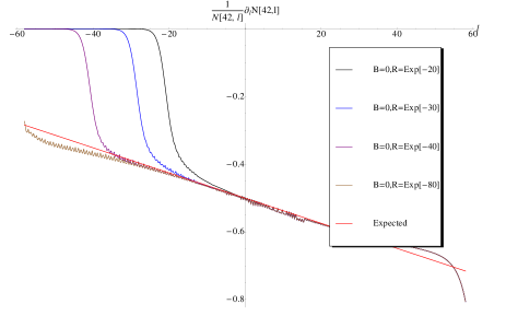
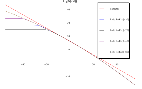
Fig. 1-a	Fig. 1-b

Figure 1: $\partial\ln\Big{(}{\cal N}^{BFKL}\left(l;Y\right)\Big{)}/\partial l$ (see Fig. 1-a) and $\ln\Big{(}{\cal N}^{BFKL}\left(l;Y\right)\Big{)}$ (see Fig. 1-b) for the BFKL equations (see Eq. (2.17) and Eq. (2.18) with the BFKL kernels) as function of $l$ at $Y=43$. $\bar{\alpha}_{S}$ is chosen to be equal to 0.2 and $l=\ln\left(x^{2}_{12}\,\Lambda^{2}_{QCD}\right)$. Curves correspond to different values of $R$. The red curve shows the solution of Eq. (2.23).

2.3 Numerical solution

Searching for numerical solution of Eq. (2.17) we introduce the regulator at short distances $R$ in the following way

$$\frac{\partial{\cal N}^{BFKL}\left(x_{12};Y\right)}{\partial Y}\,\,=\,\,\,\bar{\alpha}_{S}\int d^{2}x_{13}\,\frac{1}{x^{2}_{32}+R^{2}}\,\Big{\{}2\,{\cal N}^{BFKL}\left(x_{13};Y\right)\,\,-\,\,2\,\frac{x^{2}_{12}}{x^{2}_{13}\,+\,x^{2}_{23}\,+\,2\,R^{2}}{\cal N}^{BFKL}\left(x_{12};Y\right)\Big{\}}$$ (2.35)

We solve Eq. (2.35) at fixed but different $R$ making it smaller until the answer will not depend on $R$. We use the solution given by Eq. (2.23) , as a check of the accuracy of our numerical calculations. The procedure of the derivation of Eq. (2.35) from Eq. (2.17) is standard and it is described in Ref.[8] for example.

Fig. 1 shows the numerical solutions of the BFKL equations (see Eq. (2.17) and Eq. (2.35)) for $\partial\ln\Big{(}{\cal N}^{BFKL}\left(l;Y\right)\Big{)}/\partial l$ (see Fig. 1-a) and $\ln\Big{(}{\cal N}^{BFKL}\left(l;Y\right)\Big{)}$ (see Fig. 1-b) as functions of $l=\ln\left(x^{2}_{12}\,\Lambda^{2}_{QCD}\right)$ for different values of the short distance regulator $R$ at $Y=43$. Comparing these curves with the prediction of the solution of Eq. (2.23) shown in Fig. 1 by the red curve, one can see that our numerical problems are concentrated in the region of very short distances where the value of $x_{12}$ approaches $R$. However, we see that in the region $-20<l<20$ the numerical solution coincides with Eq. (2.23) with good accuracy.

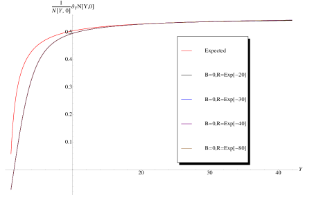
Fig. 2-a	Fig. 2-b

Figure 2: $\partial\ln\Big{(}{\cal N}^{BFKL}\left(l;Y\right)\Big{)}/\partial Y$ (see Fig. 2-a and the zoomed picture in Fig. 2-b) for the BFKL equations (see Eq. (2.17) Eq. (2.35) with the BFKL kernels) as function of $Y$ at $l=0$. $\bar{\alpha}_{S}$ is chosen to be equal to 0.2 and $l=\ln\left(x^{2}_{12}\,\Lambda^{2}_{QCD}\right)$. Curves correspond to different values of $R$. The red curve shows the solution of Eq. (2.23).

In Fig. 2 we plotted $\partial\ln\Big{(}{\cal N}^{BFKL}\left(l;Y\right)\Big{)}/\partial Y$ as a function of $Y$ for different values of $R$. Comparing the curves for different $R$ with the solution of Eq. (2.23) shown by red line in Fig. 2 one can conclude: first, that the value of the BFKL Pomeron intercept does not depend on the value of $R$ and, second, that the numerical solution reproduces quite well the analytical one, given by Eq. (2.23) . However, Fig. 2-b shows that our numerical value for the Pomeron intercept systematically above the analytical one approximately on 0.001 which we consider as a systematic error of our calculations.

3 Modified BFKL Pomeron

In this section we solve Eq. (2.17) and Eq. (2.18) in which the BFKL kernel are replaced by $K^{B}\left(x_{13},x_{32}|x_{12}\right)$. As has been mentioned above the numerical calculations in Refs.[15, 14, 16, 17] show that such a modification of the BFKL kernel leads the exponential decrease of the scattering amplitude at large values of the impact parameter. Actually, we can see this directly from the equation (see Eq. (2.16)) . Indeed, one can see that the main contribution at large $b$ stems from the region where $|\vec{b}-\vec{x}_{32}|\,\leq\,x_{12}$. At such $x_{32}$ the equation takes the form

$$\frac{\partial N\left(x_{12}\approx 2b,b;Y\right)}{\partial Y}\,\,=\,\,4\bar{\alpha}_{S}\int d^{2}x_{13}\,\frac{1}{4b^{2}}e^{-4\,B\,b^{2}-B\,x^{2}_{13}}\,2\,N\left(x_{13},0;Y\right)~{}~{}\propto~{}~{}e^{-4\,B\,b^{2}}$$ (3.36)

We can replace $\exp\left(-B\,x^{2}_{13}\right)$ by $K_{0}\left(\mu x_{13}\right)$ to reproduce correct $\exp\left(-\mu\,b\right)$ at large $b$ (see more detailed analysis of the form of the BFKL kernel in Ref.[14]). Nevertheless, we solve the equation with the kernel of Eq. (1.2) since we interested in the behaviour of the $\langle|b^{2}\left(Y,l\right)|\rangle$ versus energy for which the particular form of the kernel is not important.

The initial condition for solving Eq. (2.17) and Eq. (2.18) we take in the following form

$${\cal N}^{BFKL}\left(x_{12};Y=0\right)\,\,=\,\,\ln\left(1/\left(x^{2}_{12}\,B\right)\right);~{}~{}~{}~{}~{}~{}~{}~{}~{}~{}{\cal\widehat{N}}^{BFKL}\left(x_{12};Y=0\right)\,\,=\,\,b^{2}_{0}\,\ln\left(1/\left(x^{2}_{12}\,B\right)\right);$$ (3.37)

with $b^{2}_{0}=1/B$.

It should be stressed that Eq. (2.20) follows from the calculation of the amplitude for dipole- dipole scattering calculated in the Born Approximation of perturbative QCD. Introducing cutoff $B$ we still consider the same initial conditions, that follows from the perturbative QCD calculation, since our main goal to study the influence of the evolution in Y with the modified kernel of Eq. (1.2) on the behaviour of the scattering amplitude at large $b$.

It should be stressed that using the initial conditions of Eq. (3.37) one can see that introducing $\tilde{x}^{2}_{ik}\,=\,B\,x^{2}_{ik}$ the modified kernel takes the form

$$K^{B}\left(x_{13},x_{32}|x_{12}\right)\,\,\longrightarrow\,\,K^{1}\left(\tilde{x}_{13},\tilde{x}_{32}|\tilde{x}_{12}\right)$$ (3.38)

while the initial conditions of Eq. (3.37) can be re-written as ${\cal N}^{BFKL}\left(\tilde{x}_{12};Y=0\right)\,\,=\,\,\ln\left(1/\left(\tilde{x}^{2}_{12}\right)\right)$.

Therefore, in $\tilde{x}_{ik}$ the equation and the initial conditions have the same form for any values of $B$. However, we prefer to solve equations with the kernel $K^{B}\left(x_{13},x_{32}|x_{12}\right)$ using the $B$ independence of the solution as the way to check the accuracy of our calculations. For numerical solution we again introduce the short distance regulator in the same way as in Eq. (2.35) replacing $K^{B}\left(x_{13},x_{32}|x_{12}\right)$ by the following expression

$$\int d^{2}x_{13}K^{B}_{R}\left(x_{13},x_{32}|x_{12}\right)\,{\cal N}^{BFKL}\left(x_{12};Y\right)\,\,\equiv\,\,$$

$$~{}~{}~{}~{}~{}~{}~{}~{}~{}~{}~{}\int d^{2}x_{13}\,\frac{e^{-B\left(x^{2}_{13}\,+\,x^{2}_{32}\right)}}{x^{2}_{32}+R^{2}}\,\Big{\{}2\,{\cal N}^{BFKL}\left(x_{13};Y\right)\,\,-\,\,2\,\frac{x^{2}_{12}}{x^{2}_{13}\,+\,x^{2}_{23}\,+\,2\,R^{2}}{\cal N}^{BFKL}\left(x_{12};Y\right)\Big{\}}$$

3.1 Pomeron intercept

3.1.1 Numerical solution for the Pomeron inrtercept

In Fig. 3 it shown the solution to Eq. (2.17) with $K^{B}_{R}\left(x_{13},x_{32}|x_{12}\right)$ for different values of $B$. One can see that ${\cal N}\left(x_{12};Y\right)$ grows as $\exp\left(\omega_{0}\,Y\right)$ and the solution does not depend on the value of $B$. In this figure we do not show the dependence on the value of the regulator $R$ but we actually studied this dependence in the same way as for solution to the BFKL equation and saw that the solution does not depend on the value of $R$ . To see the power-like dependence of the solution in a clearer way we plot in Fig. 4 $d\ln\left({\cal N}\left(x_{12};Y\right)\right)/dY$ . We see that the value of the intercept is smaller than the BFKL intercept but it is still increasing approaching this value. In Fig. 5 we show that $l$ dependence of the intercept is very similar to the BFKL Pomeron.

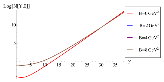
Figure 3: The solutions to Eq. (2.17) with $K^{B}_{R}\left(x_{13},x_{32}|x_{12}\right)$ for ${\cal N}\left(x_{12};Y\right)$ as function of $Y$. $\bar{\alpha}_{S}$ is chosen to be equal to 0.2. $l=\ln\left(x^{2}_{12}\,B\right)=0$. For the equation with the BFKL kernel ($B=0$ in the figure) $l=\ln\left(x^{2}_{12}\,\Lambda_{QCD}^{2}\right)=0$

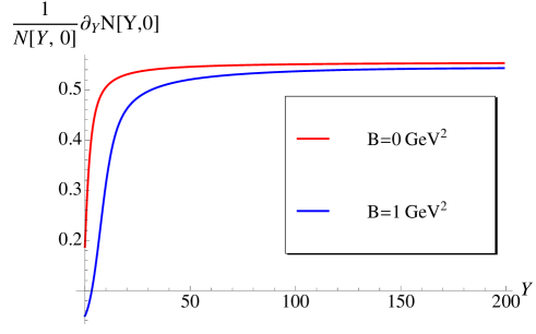
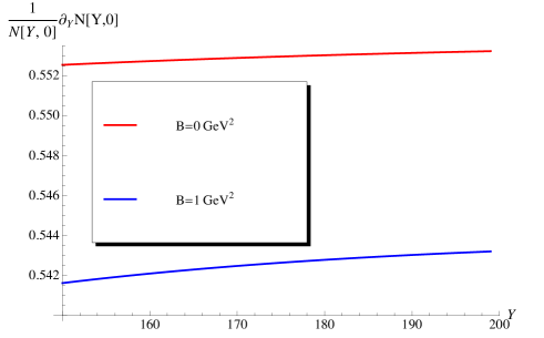
Fig. 4-a	Fig. 4-b

Figure 4: $d\,\ln{\cal N}\left(x_{12};Y\right)\big{/}dY$ for the solutions to Eq. (2.17) with $K^{B=1}_{R}\left(x_{13},x_{32}|x_{12}\right)$ as function of $Y$. $\bar{\alpha}_{S}$ is chosen to be equal to 0.2. $l=\ln\left(x^{2}_{12}\,B\right)=0$. For the equation with the BFKL kernel ($B=0$ in the figure) $l=\ln\left(x^{2}_{12}\,\Lambda_{QCD}^{2}\right)=0$

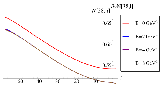
Figure 5: $d\,\ln{\cal N}\left(x_{12};Y\right)\big{/}dY$ for the solution Eq. (2.17) with $K^{B}_{R}\left(x_{13},x_{32}|x_{12}\right)$ as function of $l$. $\bar{\alpha}_{S}$ is chosen to be equal to 0.2. $l=\ln\left(x^{2}_{12}\,B\right)$. For the equation with the BFKL kernel ($B=0$ in the figure) $l=\ln\left(x^{2}_{12}\,\Lambda_{QCD}^{2}\right)=0$. $Y=38$.

3.1.2 Variational method

The numerical solution suggests that the intercept of the Pomeron at $B\neq 0$ is the same as for the BFKL Pomeron. This fact as well as the influence of cutoff $B$ on $\omega_{0}$ can be understood from the BFKL kernel in $\gamma$-representation (see Eq. (2.4)). Indeed, this kernel appears in the calculation as the following integral ( see Refs.[11, 10, 8])

$$\chi\left(\gamma,0\right)\,\,=\,\,\int\limits_{0}^{1}dt\,\frac{t^{\gamma-1}}{1-t}+\int\limits_{1}^{\infty}dt\frac{t^{\gamma-1}}{t-1}-\int\limits_{0}^{\infty}\frac{1}{t}\,\left[\frac{1}{|t-1|}-\frac{1}{\sqrt{4\,t^{2}+1}}\right]$$ (3.40)

where $t\,=\,x^{2}_{13}/x^{2}_{12}$.

The first term describes the increase of the dipole size due to evolution while the second one corresponds to normal DGLAP evolution in which the dipoles sizes decreases with the growth of $Y$. Introducing the modified BFKL kernel we cut the sizes of the intermediate dipoles such that $\tilde{x}^{2}_{13}\,\leq\,1$ ($t\leq 1/\tilde{x}^{2}_{12}$. Assuming $\tilde{x}^{2}_{12}\,\leq\,1$ we see that we do not change integration over $t\,<\,1$ but $t$ should be smaller than $t\,\leq\,1/\tilde{x}^{2}_{12}$. Therefore, we can estimate the modified kernel using

$$\chi\left(\gamma,0;\tilde{x}_{12}\right)\,\,=\,\,\int\limits_{0}^{1}dt\,\frac{t^{\gamma-1}}{1-t}+\int\limits_{1}^{1/\tilde{x}^{2}_{12}}dt\frac{t^{\gamma-1}}{t-1}-\int_{0}^{1/\tilde{x}^{2}_{12}}\frac{1}{t}\,\left[\frac{1}{|t-1|}-\frac{1}{\sqrt{4\,t^{2}+1}}\right]$$ (3.41)

Introducing the variable $t=\tilde{x}^{2}_{12}/\tilde{x}^{2}_{12}$ which is smaller that 1, we can re-write Eq. (3.41) in the form

$$\chi\left(\gamma,0;\tilde{x}_{12}\right)\,\,=\,\,\int\limits_{0}^{1}dt\,\frac{t^{\gamma-1}\,-\,1}{1\,-\,t}+\int\limits_{\tilde{x}^{2}_{12}}^{1}dt\frac{t^{-\gamma}\,-\,1}{1\,-\,t}\,+\,\int^{\infty}_{1/\tilde{x}^{2}_{12}}\frac{dt}{t\,\sqrt{4\,t^{2}+1}}$$ (3.42)

Taking the integral we obtain

$$\chi\left(\gamma,0;\tilde{x}_{12}\right)\,\, = \,\,\chi^{BFKL}\left(\gamma,0\right)\,+\,\mbox{arccsch}\left(2/\tilde{x}^{2}_{12}\right)\,-\,B\left(\tilde{x}_{12};1-\gamma,0\right)\,-\,\ln\left(1-\tilde{x}^{2}_{12}\right)$$ (3.43)

where $B\left(\tilde{x}_{12};1-\gamma,0\right)$ is incomplete $B$ function and $\chi^{BFKL}\left(\gamma,0\right)$ is given by Eq. (2.4).

One can see that Eq. (3.43) depends on $x^{2}_{12}$ through $\tilde{x}_{12}$ and, therefore, $\omega_{0}\left(\gamma,0,\tilde{x}_{12}\right)\,=\,\bar{\alpha}_{S}\,\chi\left(\gamma,0;\tilde{x}_{12}\right)$ cannot be the intercept of the Pomeron since the intercept cannot depend on the sizes of dipoles. However, we can use Eq. (3.43) for developing the estimate in the variational approach for finding the ground state (the maximal intercept). Indeed, if we introduce

$${\cal N}^{BFKL}\left(x_{12};Y\right)\,\,=\,\,\int\frac{d\omega}{2\pi i}\,e^{\omega{\cal Y}}\,\Psi\left(\tilde{x}_{12},\omega\right)$$ (3.44)

the equation looks as

$$\omega\Psi\left(\tilde{x}_{12},\omega\right)\,\,=\,\,\int d^{2}\tilde{x}_{13}\,K^{B}\left(\tilde{x}_{13},\tilde{x}_{23}|x_{12}\right)\Psi\left(\tilde{x}_{13},\omega\right)$$ (3.45)

where the r.h.s. of the equation has been discussed in Eq. (3). For the BFKL equation the eigenfunction $\Psi_{BFKL}\left(x_{13},\omega\right)=\left(x^{2}_{13}\right)^{\gamma-1}$ and the eigenvalue is given by Eq. (2.4). This function cannot be a eigenfunction of Eq. (3.44) at $B\neq 0$ as we have discussed. However, we can use this BFKL eigenfunction as a trial function in the variational method for searching the maximal value of the intercept. Actually, we use as the trial function

$$\Psi_{tr}\left(\tilde{x}_{12},\gamma\right)\,\,=\,\,\Psi_{BFKL}\left(x_{12},\gamma\right)\,\Theta\left(1-\tilde{x}^{2}_{12}\right)\,\,=\,\,\left(\tilde{x}^{2}_{12}\right)^{\gamma-1}\,\Theta\left(1-\tilde{x}^{2}_{12}\right)$$ (3.46)

The variational principle has the following form for the problem of finding the maximal intercept

$$\omega_{max}\,\,\geq\,\,\omega\left(\gamma\right)\,\, = \,\,\frac{\int d^{2}\tilde{x}_{12}\Psi^{*}_{tr}\left(\tilde{x}_{12},\gamma\right)\int d^{2}\tilde{x}_{13}\,K^{B}\left(\tilde{x}_{13},\tilde{x}_{23}|x_{12}\right)\Psi_{tr}\left(\tilde{x}_{13},\gamma\right)}{\int d^{2}\tilde{x}_{12}\,\Psi^{*}_{tr}\left(\tilde{x}_{12},\gamma\right)\,\Psi_{tr}\left(\tilde{x}_{12},\gamma\right)}$$ (3.47)

$$= \frac{\int d^{2}\tilde{x}_{12}\,\Psi^{*}_{tr}\left(\tilde{x}_{12},\gamma\right)\,\chi\left(\gamma,0;\tilde{x}_{12}\right)\Psi_{tr}\left(\tilde{x}_{12},\gamma\right)}{\int d^{2}\tilde{x}_{12}\,\Psi^{*}_{tr}\left(\tilde{x}_{12},\gamma\right)\,\Psi_{tr}\left(\tilde{x}_{12},\gamma\right)}$$

From convergency of $\int d^{2}\tilde{x}_{12}\,\Psi^{*}_{tr}\left(\tilde{x}_{12},\gamma\right)\,\Psi_{tr}\left(\tilde{x}_{12},\gamma\right)$ we conclude that $\gamma\geq 0.5$.

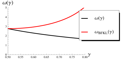
Figure 6: $\omega\left(\gamma\right)$ (see Eq. (3.47)) and $\ om_{BFKL}\left(\gamma\right)$(see Eq. (2.4)) versus $\gamma$( black and red lines, respectively). In this figure we redefine $\omega$ dividing it by $\bar{\alpha}_{S}$.

From Fig. 6 we see that $\omega(\gamma=1/2)$ coincide with the BFKL value. In other words, we prove that the resulting maximal $\omega$ can be either equal to the BFKL one or larger than the BFKL value.

3.1.3 Semi-classical solution

Examining the property of the solution to the modified BFKL equation we wish to find a semi-classical solution to this equation searching it in the form:

$$N\left({\cal Y};l\right)\,\,=\,\,e^{S\left({\cal Y},l\right)}\,\,=\,\,e^{\omega\left({\cal Y},l\right)Y\,\,+\,\,\left(\gamma\left({\cal Y},l\right)-1|\right)l}~{}\,\mbox{where}~{}~{}\omega\left({\cal Y},l\right)\,=\,\frac{\partial S\left({\cal Y};l\right)}{\partial{\cal Y}};~{}~{}\gamma\left({\cal Y},l\right)\,-\,1\,=\,\frac{\partial S|\left({\cal Y};l\right)}{\partial l}$$ (3.48)

with smooth functions $\omega\left({\cal Y},l\right)$ and $\gamma\left({\cal Y},l\right)$.

Inserting Eq. (3.48) to the equation we obtain:

$$\omega\left({\cal Y},l\right)\,-\,\chi\left(\gamma,0,x^{2}_{12}\right)\,\,=\,\,0$$ (3.49)

Deriving Eq. (3.49) we use that $\gamma$ is a smooth function and performing the integral of Eq. (3.42) we can consider $\gamma$ as being a constant. Since the equation is the first order differential equation in respect to $Y$ the condition for applying the semi-classical approach looks as follows

$$\frac{\partial\gamma\left({\cal Y};l\right)/\partial l}{\left(1-\gamma\left({\cal Y},l\right)\right)^{2}}\,\,\ll\,\,1;~{}~{}~{}~{}~{}~{}~{}~{}~{}~{}l\,\frac{\partial\gamma\left({\cal Y};l\right)}{\partial l}\,\,\ll\,\,1$$ (3.50)

where $l\,=\,\ln\left(x^{2}_{12}/\Lambda_{QCD}\right)$.

It is known[38] that for the equation in the form

$$F\left({\cal Y},l,S,\,\gamma,\omega\right)\,\,=\,\,0$$ (3.51)

we can introduce the set of characteristic lines : $l(t),{\cal Y}(t),S(t)$, $\omega(t)$ and $\gamma(t)$ which are the functions of the variable $t$ ( artificial time), that satisfy the following equations:

$$(1.)\,\,\,\,\frac{dl}{d\,t}\,\,=\,\,F_{\gamma}\,\,=\,\,-\frac{d\chi\left(\gamma,0,l\right)}{d\gamma}$$

$$(2.)\,\,\,\,\,\,\,\frac{d{\cal Y}\left(t\right)}{d\,t}\,\,=\,\,F_{\omega}\,\,=\,\,1\,\,\,\,\,\,\,$$

$$(3.)\,\,\,\,\frac{dS}{d\,t}\,\,=\,\,\gamma\,F_{\gamma}\,+\,\omega\,F_{\omega}\,\,=\,\,\,\,-\left(\gamma-1\right)\frac{\partial\chi\left(\gamma,0,l\right)}{\partial\gamma}\,\,+\,\,\omega$$

$$(4.)\,\,\,\,\frac{d\,\gamma}{d\,t}\,\,=\,\,-(\,F_{l}\,+\,\gamma\,F_{S}\,)\,\,=\,\,\frac{\partial\chi\left(\gamma(t),0,l(t)\right)}{\partial\,l}$$ (3.52)

The fifth equation is Eq. (3.49).

First, we see two thing which simplify a bit the equation: we can consider $t={\cal Y}$ and dividing Eq. (3.1.3)- 4 by Eq. (3.1.3)-1 we see that

$$\frac{d\,\gamma}{d\,l}\,\,=\,\,-\frac{\frac{\partial\chi\left(\gamma(t),0,l(t)\right)}{\partial\,l}}{\frac{d\chi\left(\gamma,0,l(t)\right)}{d\gamma}}\,\,$$ (3.53)

We solve this equation putting $\gamma\left(l=\infty\right)$ which coincide with the solution to the BFKL , as the initial condition. Due to convergency of the integral for the norm of $N$ we know that $\gamma\left(\infty\right)\,\geq\,0.5$.

The second step after finding $\gamma\left(l\right)$ is to solve Eq. (3.1.3)-1 to find the form of trajectories. It tuns out that we do not need to find $l\left({\cal Y}\right)$ as a function of ${\cal Y}$ for finding the values of $\omega$.

The last the third step is to find from Eq. (3.49) the value of $\omega$. In Fig. 7 we plot function $\gamma\left(l\right)$ for different $\gamma_{\infty}\,=\,\gamma\left(l=\infty\right)$, while Fig. 8 shows the dependence of $\omega\left(\gamma\right)\,=\,\omega\left({\cal Y},l\right)\,-\,\chi\left(\gamma,0,l\right)$ versus $l$.

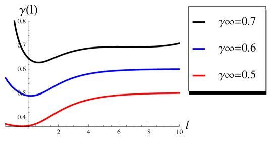
Figure 7: The trajectories of Eq. (3.49) at different values of $\gamma\left(\infty\right)$

From Fig. 8 one can see that the values of $\omega\left(\gamma\left(l\right)\right)$ does not depend on $l$ and these values turn out to be smaller or equal to the values of the intercept for the BFKL equation.

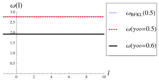
Figure 8: $\omega\left(l\right)$ versus $l$ at different values of $\gamma\left(\infty\right)$. Notice that $\omega_{\mbox{\tiny BFKL}}\left(0.5\right)$ (blue line) and $\omega\left(\gamma_{\infty}=0.5\right)$ (red dotted line) are the same.

In Fig. 9 we plot the ratio $d\gamma\left(l\right)/dl\Big{/}\left(1-\gamma\left(l\right)\right)^{2}$ and the product $ld\gamma\left(l\right)/dl$ as a function of $l$. One can see that both of these observables turn out to be small and, therefore, we can trust the semi-classical approach.

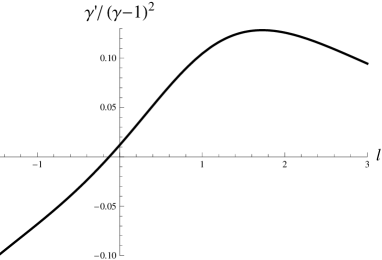
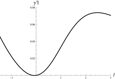
Fig. 9-a		Fig. 9-b

Figure 9: The ratio $d\gamma\left(l\right)/dl\Big{/}\left(1-\gamma\left(l\right)\right)^{2}$ (see Fig. 9-a) and the product $l\,d\gamma\left(l\right)/dl$ (see Fig. 9-b) versus $l$ for $\gamma\left(\infty\right)=0.5$.

Concluding this subsection we see that the semi-classical approach leads to $\omega\,=\,\omega_{BFKL}$.

3.1.4 Diffusion approximation

In direct analogy with the BFKL equation we develop in this section the diffusion approximation to the modified BFKL equation. The main idea of this approximation is to introduce a new function

$$\bar{N}\left({\cal Y},l\right)\,\,=\,\,e^{\frac{1}{2}\,l}N\left({\cal Y},l\right)\,\,=\,\,\int^{\epsilon+i\infty}_{\epsilon-i\infty}\frac{d\omega}{2\pi i}e^{\omega\,{\cal Y}}\,\bar{n}\left(\omega,l\right)\,\,=\,\,\int^{\epsilon+i\infty}_{\epsilon-i\infty}\frac{d\omega}{2\pi i}\int^{i\epsilon+\infty}_{i\epsilon-\infty}\frac{d\nu}{2\pi i}\bar{n}\left(\omega,\nu\right)\,e^{\omega\,{\cal Y}\,+\,i\nu l}$$ (3.54)

The diffusion approximation means that we can reduce the modified BFKL equation to the differential equation using the following expansion for $\bar{n}\left(\omega,l\right)$:

$$\bar{n}\left(\omega,l^{\prime}\right)\,\,=\,\,\bar{n}\left(\omega,l\right)\,\,+\,\,\frac{\partial\bar{n}\left(\omega,l^{\prime}\right)}{\partial l^{\prime}}|_{l^{\prime}=l}\left(l^{\prime}-l\right)\,\,+\,\,\frac{1}{2}\frac{\partial^{2}\bar{n}\left(\omega,l^{\prime}\right)}{\partial l^{\prime 2}}|_{l^{\prime}=l}\left(l-l\right)^{2}\,+\,\dots$$ (3.55)

The equation takes the form after plugging in Eq. (3.55) into Eq. (3.45)

$$\left(\omega\,-\,\Delta\left(l\right)\right)\bar{n}\left(\omega,l\right)\,\,-\,d1\left(l\right)\,\frac{\partial\bar{n}\left(\omega,l\right)}{\partial l}\,\,-\,\,\frac{1}{2}d2\left(l\right)\,\frac{\partial^{2}\bar{n}\left(\omega,l\right)}{\partial l^{2}}\,\,=\,\,0$$ (3.56)

Functions $\Delta\left(l\right)$,$d1\left(l\right)$  and $d2\left(l\right)$ can be expressed through the kernel $\chi\left(\frac{1}{2}+i\nu,0,e^{\frac{1}{2}l}\right)$ that has been introduced in Eq. (3.43), viz,

$$\Delta\left(l\right)=\chi\left(\frac{1}{2},0,e^{\frac{1}{2}l}\right);~{}~{}~{}d1\left(l\right)=-i\frac{\partial\chi\left(\frac{1}{2}+i\nu,0,e^{\frac{1}{2}l}\right)}{\partial\nu}|_{\nu=0};~{}~{}~{}d2\left(l\right)=-\frac{\partial^{2}\chi\left(\frac{1}{2}+i\nu,0,e^{\frac{1}{2}l}\right)}{\partial\nu}^{2}|_{\nu=0}.$$ (3.57)

Fig. 10 shows these functions.

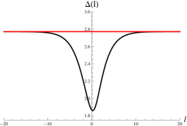
Fig. 10-a	Fig. 10-b	Fig. 10-c

Figure 10: Functions $\Delta\left(l\right)$, $d1\left(l\right)$ and $d2\left(l\right)$ versus $l$. The red line shows the BFKL value for $\omega_{\mbox{\tiny BFKL}}\left(l\right)\,\,=\,\,4\ln 2$.

Introducing $\bar{n}\left(\omega,l\right)\,\,=\,\,\exp\left(\phi\left(\omega,l\right)\right)$ for function $\phi$ Eq. (3.56) reduces to

$$\left(\omega\,-\,\Delta\left(l\right)\right)\,\,=\,\,d1\left(l\right)\gamma\left(\omega,l\right)\,\,+\,\,\frac{1}{2}d2\left(l\right)\,\left(\frac{\partial\gamma\left(\omega,l\right)}{\partial l}\,+\,\gamma^{2}\left(\omega,l\right)\right)$$ (3.58)

where $\gamma\,=\,\frac{\partial\phi\left(\omega,l\right)}{\partial l}$.

For $l\to-\infty$ $\Delta\left(l\right)\to\omega_{\mbox{\tiny BFKL}}$, $d1\left(l\right)\to 0$ and $d2\left(l\right)\,\to\,D_{0}$(see Eq. (2.22)).

Therefore, for large and negative $l$ the solution for

$$\gamma\left(\omega,l\right)\,\xrightarrow{|l|\,\gg\,1}\,\sqrt{\left(\omega-\omega_{\mbox{\tiny BFKL}}\right)/(2D_{0})}.$$ (3.59)

These values give us the initial condition for Eq. (3.58).

Solving Eq. (3.58) numerically we see that for all $\omega\,\leq\,\omega_{\mbox{\tiny BFKL}}$ $\gamma\leq 0$ at $l\to+\infty$. Such $\gamma$ lead to the amplitude $\bar{n}$ which normalization is convergent integral, namely,

$$\int dl|\bar{n}\left(\omega,l\right)|^{2}\,dl\,\,<\,\,\infty$$ (3.60)

while for $\omega\,>\,\omega_{\mbox{\tiny BFKL}}$ $\gamma$ at large $l>0$ is positive and the integral in Eq. (3.60) is divergent (see Fig. 11).

In other words, our spectrum of $\omega$ is continuous with $\omega\,\leq\,\omega_{\mbox{\tiny BFKL}}$.

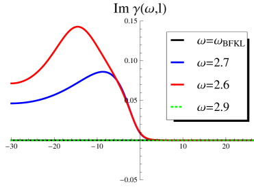
Fig. 11-a	Fig. 11-b

Figure 11: Solution to Eq. (3.58) with the initial condition of Eq. (3.59) versus $l$: Fig. 11-a for $\mbox{Re}\gamma\left(\omega,l\right)$ and Fig. 11-b for $\mbox{Im}\gamma\left(\omega,l\right)$.

3.2 Pomeron slope

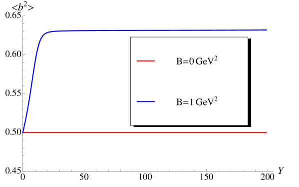
Figure 12: $\langle|b^{2}\left(Y,l\right)|\rangle$ versus $Y$ at different values of $B$ (see Eq. (1.2)). $\bar{\alpha}_{S}=0.2$. For both $B=0$ and $B=1GeV^{2}$ we took $b_{0}$ in Eq. (2.26) and Eq. (3.37) the same and equal to $0.5\,GeV^{-2}$.

Approaching the problem of calculation of $\langle|b^{2}|\rangle$, the first observation that we can make is that Eq. (2.18) is valid also for the modified BFKL kernel. Indeed, the kernel itself does not depend on the impact parameter and functions $E^{n,\gamma}\left(\rho_{1a},\rho_{2a}\right)$ is the complete set of functions. As we noticed in derivation of Eq. (2.18) the term in $\Big{\{}\dots\Big{\}}$ in Eq. (2.19) vanishes due to invariance of function $E^{n=0,\gamma}\left(\rho_{1a},\rho_{2a}\right)$ with respect to transformation $\vec{b}\,\to\,-\,\vec{b}$. Since $\omega\left(\gamma,n\right)\,\leq\,0$ for $n\,\geq\,1$ the only component of the arbitrary function of the initial condition that survives at large $Y$ is its projection on $E^{n=0,\gamma}\left(\rho_{1a},\rho_{2a}\right)$ . For this projection the term of Eq. (2.19) vanishes leading to Eq. (2.18).

Solving Eq. (2.18) with the kernel of Eq. (1.2) we calculate (see Eq. (2.15)) $\langle|b^{2}|\rangle$ as function of $Y$ (see Fig. 12). In the Reggeon approach this value gives the information on the slope of the Pomeron trajectory ($\alpha^{\prime}_{I\!\!P}$) since $\langle|b^{2}|\rangle\,\,\xrightarrow{Y\,\gg\,1}\,\,4\,\alpha^{\prime}_{I\!\!P}\,Y$. One can see from Fig. 12 that $\langle|b^{2}|\rangle$ does not depend on $Y$ at large values of $Y$. Actually, the solution to the modified BFKL equations shows a weak $Y$ dependence (see Fig. 13 which is zooomed Fig. 12). However, even if we assume that $\langle|b^{2}|\rangle|_{B=1}\,=\,4\alpha^{\prime}_{I\!\!P}Y$ the value of $\alpha^{\prime}_{I\!\!P}\,\,\leq\,\,0.510^{-5}\,b_{0}$ is extremely small. Hence we can conclude that the modified BFKL Pomeron has $\alpha^{\prime}_{I\!\!P}\,\approx\,0$.

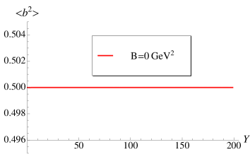
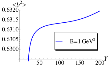
Figure 13: $\langle|b^{2}\left(Y,l\right)|\rangle=4\alpha^{\prime}_{I\!\!P}\,Y$ versus $Y$ at different values of $B$ (see Eq. (1.2)). $\bar{\alpha}_{S}=0.2$.

This result was expected and its explanation based on the general features of QCD. The general origin of the increase of $\langle|b^{2}|\rangle$ with $Y$ ( The relation: $\langle|b^{2}|\rangle\,=\,4\alpha^{\prime}_{I\!\!P}Y$) , was understood in 70’s by V.N.Gribov (Gribov’s diffusion [42]). Each emission leads to change in impact parameter by $\Delta b^{2}=1/p^{2}_{T}$ where $p_{T}$ is the typical transverse momentum. After $n$ emission $\langle b^{2}_{n}\rangle\,\,=\,\,\Delta b^{2}\,n$ which corresponds to the random walk in the transverse plane. Since the number of emission is proportional to $Y$ we obtain $\langle|b^{2}|\rangle\,\propto\,Y$. In the parton model the typical $p_{T}$ is independent of $Y$ and, therefore, we see that diffusion in $b$ leads to $\alpha_{I\!\!P}\,\neq\,0$. However, in QCD average $p_{T}$ depends on $Y$. Such dependence stems from the diffusion in $\ln p_{T}$ which means that in each emission of gluons $\ln p_{T}$ changes by a constant. Being a general features of all theories with dimensionless coupling such diffusion in $\ln p_{T}$ comes out from the BFKL equation leading to $\langle\ln^{2}\left(p^{2}_{T}/p^{2}_{0.T}\right)\,=\,4D_{0}\,Y$ (see Eq. (2.22)). From this formula one can see that we see two different branches in the BFKL equation: one leads to a rapid increase of the typical transverse momentum while another to a steep decrease. This decrease does not influence the calculation of the average $p_{T}$, resulting in $\alpha^{\prime}_{I\!\!P}=0$ for the BFKL equation. Modeling confinement by introducing cutoff in the sizes of produced dipoles we prohibit the decrease of the typical transverse momenta of the emitted gluon. As a result, the only diffusion in the large transverse momenta occurs leading to negligible $\alpha^{\prime}_{I\!\!P}$.

Fig. 14 shows the dependence of $\langle|b^{2}\left(Y,l\right)|\rangle$ on $l=\ln\left(x^{2}_{12}\,B\right)$ at $B=1\,GeV^{2}$. We can see that the dependence of $\langle|b^{2}\left(Y,l\right)|\rangle$ on $l$ is rather weak except the region of $l$ close to 0. The maximum at $l=0$ stems from Gribov’s diffusion during the first several emissions until the average $p_{T}$ grows to a considerable value.

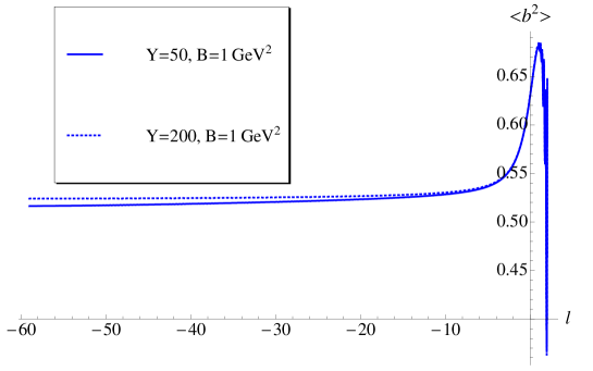
Figure 14: $\langle|b^{2}\left(Y,l\right)|\rangle$ versus $l=\ln\left(x^{2}_{12}\,B\right)$ at different values of $Y$. Solid line describes $Y=50$ while the dotted one corresponds to $Y=200$. $\bar{\alpha}_{S}=0.2$.

3.3 Saturation momentum

We have demonstrated that the modified Pomeron has a correct behaviour at large $b$ but violates the $s$-channel unitarity (Froissart theorem[9]) both for the partial amplitudes and for the total cross section, since they are proportional to $s^{\omega_{\mbox{\tiny{BFKL}}}}$. Therefore, we need to develop the CGC/saturation approach[5, 6, 7, 8] and reference therein), based on the modified BFKL Pomeron to obtain the amplitude that will satisfy the unitarity constraints. We are going to develop such an approach but in this paper we wish to use the well known feature of the CGC/saturation approach: the energy behaviour of the new dimensional scale (saturation moment) can be found from the linear equation (see Refs.[5, 39, 40]). This scale is the solution of the equation

$$N^{BFKL}\left(\frac{2}{Q_{s}\left(Y\right)};Y\right)\,\,=\,\,\frac{4}{Q^{2}_{s}\left(Y\right)}\,{\cal N}^{BFKL}\left(\frac{2}{Q_{s}\left(Y\right)};Y\right)\,\,=\,\,{\cal N}_{0}\,\,\leq\,\,1\,\,\,\,~{}~{}\mbox{where}~{}~{}~{}~{}~{}~{}~{}~{}~{}{\cal N}_{0}\,\,=\,\,\mbox{Const}$$ (3.61)

For the BFKL equation the solution to Eq. (3.61) is known. It takes the form

$$l_{s}\left(Y\right)\,\,\equiv\,\,\ln\Big{(}Q^{2}_{s}(Y)\Big{/}Q^{2}_{s}(Y_{0})\Big{)}\,\,=$$ (3.62)

$$\frac{\omega(\gamma_{cr})}{1-\gamma_{cr}}\,\,(Y-Y_{0})\,\,-\,\,\frac{3}{2(1-\gamma_{cr})}\,\ln(Y/Y_{0})\,-\,\frac{3}{(1-\gamma_{cr})^{2}}\,\sqrt{\frac{2\,\pi}{\omega^{\prime\prime}(\gamma_{cr})}}\,\Big{(}\frac{1}{\sqrt{Y}}\,-\,\frac{1}{\sqrt{Y_{0}}}\Big{)}$$

where $Y=\ln(1/x)$ is our energy variable, $\omega^{\prime\prime}(\gamma)=d^{2}\omega(\gamma)/(d\gamma)^{2}$, the value of $\gamma_{cr}$ can be found from the equation [5, 39]:

$$\frac{\omega(\gamma_{cr})}{1-\gamma_{cr}}\,\,\,=\,\,\,-\,\,\frac{d\omega(\gamma_{cr})}{d\gamma_{cr}}\,,\,\,\mbox{with}\,\,\,\,\omega\left(\gamma\right)\,\,=\,\,\bar{\alpha}_{S}\chi\left(\gamma\right)\,=\,\bar{\alpha}_{S}\left(2\,\psi\left(1\right)\,-\,\psi\left(\gamma\right)\,-\,\psi\left(1-\gamma\right)\right)$$ (3.63)

where $\psi\left(\gamma\right)\,=\,d\ln\Gamma\left(\gamma\right)/d\gamma$ and $\Gamma\left(\gamma\right)$ is the Euler gamma function. In Eq. (3.62) the first term was found in Ref.[5], the second in Ref.[39] and the third term was calculated in Ref.[40]. The solutions to Eq. (3.61) for different values of ${\cal N}_{0}$ are plotted in Fig. 15. Two features are clear from Fig. 15: Eq. (3.62) is in a good agreement with the numerical solutions; and the energy dependences of the saturation scales are the same for the BFKL equation and for the modified BFKL equation which includes confinement.

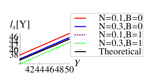
Fig. 15-a	Fig. 15-b

Figure 15: $l_{s}\left(Y\right)\,=\,\ln\Big{(}Q^{2}_{s}(Y)\Big{/}Q^{2}_{s}(Y_{0})\Big{)}$ , where $Q_{s}\left(Y\right)$ is the solution to Eq. (3.61), versus $Y$ for different values of ${\cal N}_{0}$. $\bar{\alpha}_{S}=0.2$. The red solid and dotted lines correspond to solution of the BFKL equation, the solid dark brown line describes Eq. (3.62) while the blue line is the solution to Eq. (3.61) for the modified BFKL equation.

4 Conclusions

The main goal of this paper is to find how our assumption that the size of produced dipoles cannot be large, will affect the main properties of the BFKL Pomeron. To achieve this goal we solved the BFKL equation with the modified kernel of Eq. (1.2). We found out that the modified BFKL Pomeron has the same intercept $\Delta$ as the BFKL Pomeron ( $\Delta_{\mbox{\tiny BFKL}}\,\,=\,\,\ \omega_{\mbox{\tiny BFKL}}\,\,=\,\,4\,\ln 2\bar{\alpha}_{S}$) and $\alpha^{\prime}_{I\!\!P}=0$. Therefore, the BFKL Pomeron with the modified kernel reproduces the main features of the soft Pomeron that has been found both from N=4 SYM theory[34, 35, 36, 37] and from the high energy Reggeon phenomenology[31, 32]: the large value of the Pomeron intercept ($\omega_{0}\approx\,0.2-0.3$) and $\alpha^{\prime}_{I\!\!P}=0$. These both conclusions are in agreement with the numerical solution of the modified BFKL and BK equations [15, 14].

We consider as one of the results of this paper that we developed several methods to solve the modified BFKL equation analytically (semi-classical and diffusion approximations). The fact that these methods work we checked with the numerical calculation.

Actually, we were surprised that the model for confinement changed so little in the BFKL Pomeron and on qualitative level, the Pomeron that emerges from the modified BFKL equation, looks quite the same at the BFKL Pomeron, both in parameters and in character of the energy behaviour. It seems that the only difference between the BFKL Pomeron and the modified BFKL Pomeron is that the second has a correct large impact parameter behaviour.

We believe that this statement does not depend on the particular form of Eq. (1.2). As it has been mentioned the analytical approaches that have been developed in sections 3.1.2-3.1.4 actually are based on the kernel in which $\exp\left(-Bx^{2}\right)$ is replaced by $\Theta\left(1/B-x^{2}\right)$. This approach led to the same properties as the kernel of Eq. (1.2). Considering Eq. (3.45) and introducing $E=-\omega$ one can see that Eq. (3.45) can be viewed as

$$E\,\Psi\left(x_{12},\omega\right)\,\,=\,\,{\cal H}\Psi\left(x_{12},\omega\right)$$ (4.64)

where ${\cal H}$ is a Hamiltonian ( see Eq. (3.45)).

At short distance the BFKL wave function $\Psi_{\tiny{BFKL}}\left(x_{12},\omega\right)\,\,=\,\,\left(x^{2}_{12}\right)^{-\frac{1}{2}\pm i\nu}$ is the eigenfunction of Eq. (4.64) with the eigenvalue $\omega\left(-\frac{1}{2}\pm i\nu,0\right)$. Any eigenfunction of Eq. (4.64) will have the following two limits:

$$\Psi\left(x_{12},\omega\right)\,\,\xrightarrow{x_{12}\,\to\,0}\,\,\Psi_{\tiny{BFKL}}\left(x_{12},\omega\right)\,\,\,\,\,\mbox{and}\,\,\,\,\,\,\,\,\Psi\left(x_{12},\omega\right)\,\,\xrightarrow{x_{12}\,\to\,\infty}\,\,\mbox{Const}$$ (4.65)

At first sight the condition at long distances will restrict the values of $\nu$ in the comparison with the BFKL equation. However, it is not the case. Indeed, the eigenvalues of the BFKL equation is degenerate having two eigenfunctions with positive and negative $\nu$. One can see that we can find the sum of these two eigenfunction ( $\Psi\left(x_{12},\omega\right)\,\,=\,\left(1/x^{2}_{12}\right)^{\frac{1}{2}}\sin\left(\nu/x^{2}_{12}\right)$ which tends to zero at $x_{12}\to\infty$. Therefore, at any $\nu$ we can satisfy the second condition of Eq. (4.65). On the other hand for $\nu=i\kappa\,\,(\kappa\,>\,0)$ we have two eigenfunctions: $\left(x^{2}_{12}\right)^{-\frac{1}{2}-\kappa}$ and $\left(x^{2}_{12}\right)^{-\frac{1}{2}+\kappa}$ . The normalization condition selects out the only eigenfunction $\left(x^{2}_{12}\right)^{-\frac{1}{2}+\kappa}$ which has no divergency at $x_{12}\to 0$. Using this function we cannot satisfy the condition at $x_{12}\to\infty$ and, therefore, we have no solution of Eq. (4.64) for $\nu=i\kappa$. Hence, we expect that the spectrum for the modified Hamiltonian will be the same as the BFKL spectrum. We plan to investigate different models of confinement and demonstrate that our general arguments works.

The independence of the spectrum of the BFKL Pomeron on the models for the confinement gives us a hope that the unknown confinement will change only slightly the equations of the CGC/saturation approach and these changes will not depend on the particular way of taking into account the long distances physics. In simple words, this paper gives a hope that the CGC/saturation approach will be still a theory in spite of needed model modifications due to confinement. The main ingredient of the CGC/saturation approach: the saturation momentum, can be calculated from the solution of the linear equation. Its value turns out to be the same as for the BFKL equation. This fact confirms our expectations that a modification of the BFKL kernel for correct large $b$ behaviour will not lead to a significant alteration of the CGC/saturation approach.

Eq. (2.18) is new and using this equation we are able to calculate directly $\langle|b^{2}\left(Y,l\right)|\rangle$ which gives the information on the effective slope of the resulting Pomeron. However, we have not solved the modified BFKL equation at fixed $b$. Therefore, at the moment we cannot discuss changes that the correct $b$ behaviour could trigger in azimuthal correlations that are originated by the BFKL Pomeron. However, since we introduce a new dimensional scale $B$ that cuts large distances, we can expect changes in the estimates of local anisotropy and density variation outside of the saturation region ( see Kovner’s talk [44]). Nevertheless it is too early to discuss this topic without obtaining the solution.

Our discussions with our colleagues show that we need to comment on the BFKL Pomeron with running QCD coupling. It has been intensively discussed in Refs. [43] how to satisfy the general initial conditions that are originated by confinement in the case of the BFKL Pomeron with running QCD coupling. In particular, it turns out that the confinement manifests itself in a series of the Regge poles making the entire picture close to the high energy phenomenology based on the Regge poles. However as it has been discussed in section 2, it is not enough to satisfy the initial conditions to introduce the correct impact parameter behaviour. We have to change the BFKL kernel. In the approach of Refs.[43] the initial conditions that stem from the confinement , are satisfied without making any corrections to the BFKL kernel, and this approach does not change the large impact parameter behaviour of the scattering amplitude. Thus we need to take into account the running QCD coupling in addition to the modeling of confinement in the BFKL kernel. We are planning to do this in our future publications. At the moment, it is clear that the confinement modeling provides the scale for freezing the running QCD coupling that has been introduced in all numerical solutions of the non-linear equation (see Ref.[45]).

We believe that this paper will be useful in the search of the theoretical motivated way to include the non-perturbative corrections at large values of the impact parameters as well as in understanding of the main ingredients of high energy phenomenology for soft processes. In the future publication we are going to study how the way of introducing confinement into the BFKL equation could change the features of the Pomeron and to develop the CGC/saturation approach, based on the modified BFKL Pomeron.

5 Acknowledgements

We thank our colleagues at UTFSM and Tel Aviv university for encouraging discussions. We also thank Lev Lipatov for fruitful discussions on the subject of this paper. Our special thanks go to Marat Siddikov, who participated in all discussions and in part of calculations. His contribution was very essential for us and we considered him as one of the authors. However, he declined this offer on the ground that his contribution was not sufficient. He won our respect but now we have a problem how to express our deep gratitude to him. This research was supported by the Fondecyt (Chile) grant 1100648.

References

- [1] A. Kovner and U. A. Wiedemann, Phys. Rev. D 66, 051502 (2002) [hep-ph/0112140].
- [2] A. Kovner and U. A. Wiedemann, Phys. Rev. D 66, 034031 (2002) [hep-ph/0204277].
- [3] A. Kovner and U. A. Wiedemann, Phys. Lett. B 551, 311 (2003) [hep-ph/0207335].
- [4] E. Ferreiro, E. Iancu, K. Itakura and L. McLerran, Nucl. Phys. A 710, 373 (2002) [hep-ph/0206241].
- [5] L. V. Gribov, E. M. Levin and M. G. Ryskin, Phys. Rep. 100 (1983) 1.
- [6] A. H. Mueller and J. Qiu, Nucl. Phys. B268 (1986) 427.
-
[7]
L. McLerran and R. Venugopalan,
Phys. Rev. D49 (1994) 2233, 3352; D50 (1994) 2225;
D53 (1996) 458;
D59 (1999) 094002. - [8] Yuri V Kovchegov and Eugene Levin, “ Quantum Choromodynamics at High Energies”, Cambridge Monographs on Particle Physics, Nuclear Physics and Cosmology, Cambridge University Press, 2012 and references therein.
-
[9]
M. Froissart,
Phys. Rev. 123 (1961) 1053;
A. Martin, “Scattering Theory: Unitarity, Analitysity and Crossing.” Lecture Notes in Physics, Springer-Verlag, Berlin-Heidelberg-New-York, 1969. - [10] L. N. Lipatov, Phys. Rep. 286 (1997) 131; Sov. Phys. JETP 63 (1986) 904 [Zh. Eksp. Teor. Fiz. 90, 1536 (1986)].
- [11] E. A. Kuraev, L. N. Lipatov, and F. S. Fadin, Sov. Phys. JETP 45, 199 (1977); Ya. Ya. Balitsky and L. N. Lipatov, Sov. J. Nucl. Phys. 28, 822 (1978).
- [12] H. Navelet and R. B. Peschanski, Nucl. Phys. B 507, 35 (1997).
- [13] I. Gradstein and I. Ryzhik, Table of Integrals, Series, and Products, Fifth Edition, Academic Press, London, 1994.
- [14] J. Berger and A. M. Stasto, Phys. Rev. D 84, 094022 (2011) [arXiv:1106.5740 [hep-ph]].
- [15] J. Berger and A. Stasto, Phys. Rev. D 83, 034015 (2011) [arXiv:1010.0671 [hep-ph]].
- [16] K. J. Golec-Biernat and A. M. Stasto, Nucl. Phys. B 668, 345 (2003) [hep-ph/0306279].
- [17] E. Gotsman, M. Kozlov, E. Levin, U. Maor and E. Naftali, Nucl. Phys. A 742, 55 (2004) [hep-ph/0401021].
- [18] A. Kormilitzin and E. Levin, Nucl. Phys. A 849, 98 (2011) [arXiv:1009.1468 [hep-ph]].
- [19] Y. Hatta and A. H. Mueller, Nucl. Phys. A 789, 285 (2007) [hep-ph/0702023 [HEP-PH]].
- [20] A. H. Mueller and S. Munier, Phys. Rev. D 81, 105014 (2010) [arXiv:1002.4575 [hep-ph]].
-
[21]
V. N. Gribov and L. N. Lipatov, Sov. J. Nucl. Phys 15 (1972)
438;
G. Altarelli and G. Parisi, Nucl. Phys. B 126 (1977) 298;
Yu. l. Dokshitser, Sov. Phys. JETP 46 (1977) 641. - [22] E. Gotsman, E. Levin, M. Lublinsky, U. Maor and K. Tuchin, Nucl. Phys. A 697, 521 (2002).
- [23] A. H. Mueller, Nucl. Phys. B 335, 115 (1990).
- [24] E. Levin and K. Tuchin, Nucl. Phys. B 573, 833 (2000) [hep-ph/9908317]; Nucl. Phys. A 691, 779 (2001) [hep-ph/0012167]; 693, 787 (2001) [hep-ph/0101275].
- [25] M. Braun, Eur. Phys. J. C 16, 337 (2000) [hep-ph/0001268].
- [26] N. Armesto and M. A. Braun, Eur. Phys. J. C 20, 517 (2001) [hep-ph/0104038].
- [27] M. Lublinsky, E. Gotsman, E. Levin and U. Maor, Nucl. Phys. A 696, 851 (2001) [hep-ph/0102321]; M. Lublinsky, Eur. Phys. J. C 21, 513 (2001) [hep-ph/0106112].
- [28] I. Balitsky, [arXiv:hep-ph/9509348]; Phys. Rev. D60, 014020 (1999) [arXiv:hep-ph/9812311] Y. V. Kovchegov, Phys. Rev. D60, 034008 (1999), [arXiv:hep-ph/9901281].
- [29] G. F. de Teramond and S. J. Brodsky, Phys. Rev. Lett. 102 (2009) 081601 [arXiv:0809.4899 [hep-ph]]; J. R. Forshaw and R. Sandapen, arXiv:1207.4358 [hep-ph] and references therein.
- [30] B. Z. Kopeliovich, I. K. Potashnikova, B. Povh and I. Schmidt, Phys. Rev. D 76 (2007) 094020 [arXiv:0708.3636 [hep-ph]] and references therein.
- [31] E. Gotsman, E. Levin and U. Maor, Eur. Phys. J. C 71 (2011) 1553 [arXiv:1010.5323 [hep-ph]].
- [32] A. D. Martin, M. G. Ryskin and V. A. Khoze, Eur. Phys. J. C 71, 1617 (2011) [arXiv:1102.2844 [hep-ph]] A. D. Martin, V. A. Khoze and M. G. Ryskin, Frascati Phys. Ser. 54, 162 (2012) [arXiv:1202.4966 [hep-ph]].
- [33] J. M. Maldacena, Adv. Theor. Math. Phys. 2 (1998) 231 [Int. J. Theor. Phys. 38 (1999) 1113] [arXiv:hep-th/9711200]; S. S. Gubser, I. R. Klebanov and A. M. Polyakov, Phys. Lett. B 428 (1998) 105 [arXiv:hep-th/9802109]; E. Witten, Adv. Theor. Math. Phys. 2 (1998) 505 [arXiv:hep-th/9803131].
- [34] A. V. Kotikov, L. N. Lipatov, A. I. Onishchenko and V. N. Velizhanin, Phys. Lett. B 595 (2004) 521 [Erratum-ibid. B 632 (2006) 754] [hep-th/0404092].
- [35] R. C. Brower, J. Polchinski, M. J. Strassler and C. I. Tan, JHEP 0712 (2007) 005 [arXiv:hep-th/0603115].
- [36] R. C. Brower, M. J. Strassler and C. I. Tan, arXiv:0707.2408 [hep-th].
- [37] R. C. Brower, M. J. Strassler and C. I. Tan, JHEP 0806 (2008) 048 [arXiv:0801.3002 [hep-th]].
- [38] I. N. Sneddon, “ Elements of partial differential equations”, Mc-Graw-Hill, New York,1957.
- [39] A. H. Mueller and D. N. Triantafyllopoulos, Nucl. Phys. B640 (2002) 331 [arXiv:hep-ph/0205167]; D. N. Triantafyllopoulos, Nucl. Phys. B648 (2003) 293 [arXiv:hep-ph/0209121].
- [40] S. Munier and R. B. Peschanski, Phys. Rev. D 70 (2004) 077503 [arXiv:hep-ph/0401215]; Phys. Rev. D 69 (2004) 034008 [arXiv:hep-ph/0310357]; Phys. Rev. Lett. 91 (2003) 232001 [arXiv:hep-ph/0309177].
- [41] E. M. Levin and M. G. Ryskin, Phys. Rept. 189 (1990) 267, Sov. J. Nucl. Phys. 50 (1989) 881 [Z. Phys. C 48 (1990) 231] [Yad. Fiz. 50 (1989) 1417].
- [42] V. N. Gribov, “Space-time description of hadron interactions at high-energies,” hep-ph/0006158; Sov. J. Nucl. Phys. 9 (1969) 369 [Yad. Fiz. 9 (1969) 640].
- [43] H. Kowalski, L. N. Lipatov and D. A. Ross, Phys. Part. Nucl. 44 (2013) 547 [arXiv:1205.6713 [hep-ph]]; “Indirect Evidence for New Physics at the 10 TeV Scale,” arXiv:1109.0432 [hep-ph]; H. Kowalski, L. N. Lipatov, D. A. Ross and G. Watt, Nucl. Phys. A 854, 45 (2011); Eur. Phys. J. C 70, 983 (2010) [arXiv:1005.0355 [hep-ph]].
- [44] A. Kovner, “ THE ”RIDGE” IN p-p AND p-A”, talk at Low x WS, May 30 - June 4, 2013,Rehovot-Eilat, Israel.
- [45] J. L. Albacete, N. Armesto, J. G. Milhano, C. A. Salgado and U. A. Wiedemann, Phys. Rev. D 71, 014003 (2005) [hep-ph/0408216].