Semi-Supervised
Information-Maximization Clustering

Abstract

Semi-supervised clustering aims to introduce prior knowledge in the decision process of a clustering algorithm. In this paper, we propose a novel semi-supervised clustering algorithm based on the information-maximization principle. The proposed method is an extension of a previous unsupervised information-maximization clustering algorithm based on squared-loss mutual information to effectively incorporate must-links and cannot-links. The proposed method is computationally efficient because the clustering solution can be obtained analytically via eigendecomposition. Furthermore, the proposed method allows systematic optimization of tuning parameters such as the kernel width, given the degree of belief in the must-links and cannot-links. The usefulness of the proposed method is demonstrated through experiments. lustering, Information Maximization, Squared-Loss Mutual Information, Semi-supervised.

1 Introduction

The objective of clustering is to classify unlabeled data into disjoint groups based on their similarity, and clustering has been extensively studied in statistics and machine learning. K-means [12] is a classic algorithm that clusters data so that the sum of within-cluster scatters is minimized. However, its usefulness is rather limited in practice because k-means only produces linearly separated clusters. Kernel k-means [5] overcomes this limitation by performing k-means in a feature space induced by a reproducing kernel function [15]. Spectral clustering [17, 13] first unfolds non-linear data manifolds based on sample-sample similarity by a spectral embedding method, and then performs k-means in the embedded space.

These non-linear clustering techniques is capable of handling highly complex real-world data. However, they lack objective model selection strategies, i.e., tuning parameters included in kernel functions or similarity measures need to be manually determined in an unsupervised manner. Information-maximization clustering can address the issue of model selection [1, 7, 18], which learns a probabilistic classifier so that some information measure between feature vectors and cluster assignments is maximized in an unsupervised manner. In the information-maximization approach, tuning parameters included in kernel functions or similarity measures can be systematically determined based on the information-maximization principle. Among the information-maximization clustering methods, the algorithm based on squared-loss mutual information (SMI) was demonstrated to be promising [18], because it gives the clustering solution analytically via eigendecomposition.

In practical situations, additional side information regarding clustering solutions is often provided, typically in the form of must-links and cannot-links: A set of sample pairs which should belong to the same cluster and a set of sample pairs which should belong to different clusters, respectively. Such semi-supervised clustering (which is also known as clustering with side information) has been shown to be useful in practice [22, 6, 23]. Spectral learning [9] is a semi-supervised extension of spectral clustering that enhances the similarity with side information so that sample pairs tied with must-links have higher similarity and sample pairs tied with cannot-links have lower similarity. On the other hand, constrained spectral clustering [24] incorporates the must-links and cannot-links as constraints in the optimization problem.

However, in the same way as unsupervised clustering, the above semi-supervised clustering methods suffer from lack of objective model selection strategies and thus tuning parameters included in similarity measures need to be determined manually. In this paper, we extend the unsupervised SMI-based clustering method to the semi-supervised clustering scenario. The proposed method, called semi-supervised SMI-based clustering (3SMIC), gives the clustering solution analytically via eigendecomposition with a systematic model selection strategy. Through experiments on real-world datasets, we demonstrate the usefulness of the proposed 3SMIC algorithm.

2 Information-Maximization Clustering with Squared-Loss Mutual Information

In this section, we formulate the problem of information-maximization clustering and review an existing unsupervised clustering method based on squared-loss mutual information.

2.1 Information-Maximization Clustering

The goal of unsupervised clustering is to assign class labels to data instances so that similar instances share the same label and dissimilar instances have different labels. Let $\{{\boldsymbol{x}}_{i}|{\boldsymbol{x}}_{i}\in\mathbb{R}^{d}\}_{i=1}^{n}$ be feature vectors of data instances, which are drawn independently from a probability distribution with density $p^{\ast}({\boldsymbol{x}})$. Let $\{y_{i}|y_{i}\in\{1,\ldots,c\}\}_{i=1}^{n}$ be class labels that we want to obtain, where $c$ denotes the number of classes and we assume $c$ to be known through the paper.

The information-maximization approach tries to learn the class-posterior probability $p^{\ast}(y|{\boldsymbol{x}})$ in an unsupervised manner so that some “information” measure between feature ${\boldsymbol{x}}$ and label $y$ is maximized. Mutual information (MI) [16] is a typical information measure for this purpose [1, 7]:

$$\mathrm{MI}:=\int\sum_{y=1}^{c}p^{\ast}({\boldsymbol{x}},y)\log\frac{p^{\ast}({\boldsymbol{x}},y)}{p^{\ast}({\boldsymbol{x}})p^{\ast}(y)}\mathrm{d}{\boldsymbol{x}}.$$ (1)

An advantage of the information-maximization formulation is that tuning parameters included in clustering algorithms such as the Gaussian width and the regularization parameter can be objectively optimized based on the same information-maximization principle. However, MI is known to be sensitive to outliers [3], due to the log function that is strongly non-linear. Furthermore, unsupervised learning of class-posterior probability $p^{\ast}(y|{\boldsymbol{x}})$ under MI is highly non-convex and finding a good local optimum is not straightforward in practice [7].

To cope with this problem, an alternative information measure called squared-loss MI (SMI) has been introduced [21]:

$$\mathrm{SMI} :=\frac{1}{2}\int\sum_{y=1}^{c}p^{\ast}({\boldsymbol{x}})p^{\ast}(y)\left(\frac{p^{\ast}({\boldsymbol{x}},y)}{p^{\ast}({\boldsymbol{x}})p^{\ast}(y)}-1\right)^{2}\mathrm{d}{\boldsymbol{x}}.$$ (2)

Ordinary MI is the Kullback-Leibler (KL) divergence [10] from $p^{\ast}({\boldsymbol{x}},y)$ to $p^{\ast}({\boldsymbol{x}})p^{\ast}(y)$, while SMI is the Pearson (PE) divergence [14]. Both KL and PE divergences belong to the class of the Ali-Silvey-Csiszár divergences [2, 4], which is also known as the $f$-divergences. Thus, MI and SMI share many common properties, for example they are non-negative and equal to zero if and only if feature vector ${\boldsymbol{x}}$ and label $y$ are statistically independent. Information-maximization clustering based on SMI was shown to be computationally advantageous [18]. Below, we review the SMI-based clustering (SMIC) algorithm.

2.2 SMI-Based Clustering

In unsupervised clustering, it is not straightforward to approximate SMI (2) because labeled samples are not available. To cope with this problem, let us expand the squared term in Eq.(2). Then SMI can be expressed as

$$\mathrm{SMI} =\frac{1}{2}\int\sum_{y=1}^{c}p^{\ast}({\boldsymbol{x}})p^{\ast}(y)\left(\frac{p^{\ast}({\boldsymbol{x}},y)}{p^{\ast}({\boldsymbol{x}})p^{\ast}(y)}\right)^{2}\mathrm{d}{\boldsymbol{x}}$$

$$\phantom{=}-\int\sum_{y=1}^{c}p^{\ast}({\boldsymbol{x}})p^{\ast}(y)\frac{p^{\ast}({\boldsymbol{x}},y)}{p^{\ast}({\boldsymbol{x}})p^{\ast}(y)}\mathrm{d}{\boldsymbol{x}}+\frac{1}{2}$$

$$=\frac{1}{2}\int\sum_{y=1}^{c}p^{\ast}(y|{\boldsymbol{x}})p^{\ast}({\boldsymbol{x}})\frac{p^{\ast}(y|{\boldsymbol{x}})}{p^{\ast}(y)}\mathrm{d}{\boldsymbol{x}}-\frac{1}{2}.$$ (3)

Suppose that the class-prior probability $p^{\ast}(y)$ is uniform, i.e.,

$$p(y)=\frac{1}{c}\mbox{ for }y=1,\ldots,c.$$

Then we can express Eq.(3) as

$$\frac{c}{2}\int\sum_{y=1}^{c}p^{\ast}(y|{\boldsymbol{x}})p^{\ast}({\boldsymbol{x}})p^{\ast}(y|{\boldsymbol{x}})\mathrm{d}{\boldsymbol{x}}-\frac{1}{2}.$$ (4)

Let us approximate the class-posterior probability $p^{\ast}(y|{\boldsymbol{x}})$ by the following kernel model:

$$p(y|{\boldsymbol{x}};{\boldsymbol{\alpha}}) :=\sum_{i=1}^{n}\alpha_{y,i}K({\boldsymbol{x}},{\boldsymbol{x}}_{i}),$$ (5)

where ${\boldsymbol{\alpha}}=(\alpha_{1,1},\ldots,\alpha_{c,n})^{\top}\in\mathbb{R}^{cn}$ is the parameter vector, ^⊤ denotes the transpose, and $K({\boldsymbol{x}},{\boldsymbol{x}}^{\prime})$ denotes a kernel function. Let ${\boldsymbol{K}}$ be the kernel matrix whose $(i,j)$ element is given by $K({\boldsymbol{x}}_{i},{\boldsymbol{x}}_{j})$ and let ${\boldsymbol{\alpha}}_{y}=(\alpha_{y,1},\ldots,\alpha_{y,n})^{\top}\in\mathbb{R}^{n}$. Approximating the expectation over $p^{\ast}({\boldsymbol{x}})$ in Eq.(4) with the empirical average of samples $\{{\boldsymbol{x}}_{i}\}_{i=1}^{n}$ and replacing the class-posterior probability $p^{\ast}(y|{\boldsymbol{x}})$ with the kernel model $p(y|{\boldsymbol{x}};{\boldsymbol{\alpha}})$, we have the following SMI approximator:

$$\widehat{\mathrm{SMI}} :=\frac{c}{2n}\sum_{y=1}^{c}{\boldsymbol{\alpha}}_{y}^{\top}{\boldsymbol{K}}^{2}{\boldsymbol{\alpha}}_{y}-\frac{1}{2}.$$ (6)

Under orthonormality of $\{{\boldsymbol{\alpha}}_{y}\}_{y=1}^{c}$, a global maximizer is given by the normalized eigenvectors ${\boldsymbol{\phi}}_{1},\ldots,{\boldsymbol{\phi}}_{c}$ associated with the eigenvalues $\lambda_{1}\geq\cdots\geq\lambda_{n}\geq 0$ of ${\boldsymbol{K}}$. Because the sign of eigenvector ${\boldsymbol{\phi}}_{y}$ is arbitrary, we set the sign as

$$\widetilde{{\boldsymbol{\phi}}}_{y}={\boldsymbol{\phi}}_{y}\times\mathrm{sign}({\boldsymbol{\phi}}_{y}^{\top}{\boldsymbol{1}}_{n}),$$

where $\mathrm{sign}(\cdot)$ denotes the sign of a scalar and ${\boldsymbol{1}}_{n}$ denotes the $n$-dimensional vector with all ones. On the other hand, since

$$p^{\ast}(y)=\int p^{\ast}(y|{\boldsymbol{x}})p^{\ast}({\boldsymbol{x}})\mathrm{d}{\boldsymbol{x}}\approx\frac{1}{n}\sum_{i=1}^{n}p(y|{\boldsymbol{x}}_{i};{\boldsymbol{\alpha}})={\boldsymbol{\alpha}}_{y}^{\top}{\boldsymbol{K}}{\boldsymbol{1}}_{n},$$

and the class-prior probability was set to be uniform, we have the following normalization condition:

$${\boldsymbol{\alpha}}_{y}^{\top}{\boldsymbol{K}}{\boldsymbol{1}}_{n}=\frac{1}{c}.$$

Furthermore, negative outputs are rounded up to zero to ensure that outputs are non-negative.

Taking these post-processing issues into account, cluster assignment $y_{i}$ for ${\boldsymbol{x}}_{i}$ is determined as the maximizer of the approximation of $p(y|{\boldsymbol{x}}_{i})$:

$$y_{i} =\mathop{\mathrm{argmax\,}}_{y}\frac{[\max({\boldsymbol{0}}_{n},{\boldsymbol{K}}\widetilde{{\boldsymbol{\phi}}}_{y})]_{i}}{c~{}\max({\boldsymbol{0}}_{n},{\boldsymbol{K}}\widetilde{{\boldsymbol{\phi}}}_{y})^{\top}{\boldsymbol{1}}_{n}}=\mathop{\mathrm{argmax\,}}_{y}\frac{[\max({\boldsymbol{0}}_{n},\widetilde{{\boldsymbol{\phi}}}_{y})]_{i}}{\max({\boldsymbol{0}}_{n},\widetilde{{\boldsymbol{\phi}}}_{y})^{\top}{\boldsymbol{1}}_{n}},$$

where ${\boldsymbol{0}}_{n}$ denotes the $n$-dimensional vector with all zeros, the max operation for vectors is applied in the element-wise manner, and $[\cdot]_{i}$ denotes the $i$-th element of a vector. Note that ${\boldsymbol{K}}\widetilde{{\boldsymbol{\phi}}}_{y}=\lambda_{y}\widetilde{{\boldsymbol{\phi}}}_{y}$ is used in the above derivation.

For out-of-sample prediction, cluster assignment $y^{\prime}$ for new sample ${\boldsymbol{x}}^{\prime}$ may be obtained as

$$y^{\prime} :=\mathop{\mathrm{argmax\,}}_{y}\frac{\max\left(0,\sum_{i=1}^{n}K({\boldsymbol{x}}^{\prime},{\boldsymbol{x}}_{i})[\widetilde{{\boldsymbol{\phi}}}_{y}]_{i}\right)}{\lambda_{y}\max({\boldsymbol{0}}_{n},\widetilde{{\boldsymbol{\phi}}}_{y})^{\top}{\boldsymbol{1}}_{n}}.$$ (7)

This clustering algorithm is called the SMI-based clustering (SMIC).

SMIC may include a tuning parameter, say $\theta$, in the kernel function, and the clustering results of SMIC depend on the choice of $\theta$. A notable advantage of information-maximization clustering is that such a tuning parameter can be systematically optimized by the same information-maximization principle. More specifically, cluster assignments $\{y^{\theta}_{i}\}_{i=1}^{n}$ are first obtained for each possible $\theta$. Then the quality of clustering is measured by the SMI value estimated from paired samples $\{({\boldsymbol{x}}_{i},y^{\theta}_{i})\}_{i=1}^{n}$. For this purpose, the method of least-squares mutual information (LSMI) [21] is useful because LSMI was theoretically proved to be the optimal non-parametric SMI approximator [20]; see Appendix 0.A for the details of LSMI. Thus, we compute LSMI as a function of $\theta$ and the tuning parameter value that maximizes LSMI is selected as the most suitable one:

$$\max_{\theta}\mbox{LSMI}(\theta)$$

3 Semi-Supervised SMIC

In this section, we extend SMIC to a semi-supervised clustering scenario where a set of must-links and a set of cannot-links are provided. A must-link $(i,j)$ means that ${\boldsymbol{x}}_{i}$ and ${\boldsymbol{x}}_{j}$ are encouraged to belong to the same cluster, while a cannot-link $(i,j)$ means that ${\boldsymbol{x}}_{i}$ and ${\boldsymbol{x}}_{j}$ are encouraged to belong to different clusters. Let ${\boldsymbol{M}}$ be the must-link matrix with $M_{i,j}=1$ if a must-link between ${\boldsymbol{x}}_{i}$ and ${\boldsymbol{x}}_{j}$ is given and $M_{i,j}=0$ otherwise. In the same way, we define the cannot-link matrix ${\boldsymbol{C}}$. We assume that $M_{i,i}=1$ for all $i=1,\ldots,n$, and $C_{i,i}=0$ for all $i=1,\ldots,n$. Below, we explain how must-link constraints and cannot-link constraints are incorporated into the SMIC formulation.

3.1 Incorporating Must-Links in SMIC

When there exists a must-link between ${\boldsymbol{x}}_{i}$ and ${\boldsymbol{x}}_{j}$, we want them to share the same class label. Let

$${\boldsymbol{p}}^{*}_{i}=(p^{\ast}(y=1|{\boldsymbol{x}}_{i}),\ldots,p^{\ast}(y=c|{\boldsymbol{x}}_{i}))^{\top}$$

be the soft-response vector for ${\boldsymbol{x}}_{i}$. Then the inner product $\langle{\boldsymbol{p}}^{*}_{i},{\boldsymbol{p}}^{*}_{j}\rangle$ is maximized if and only if ${\boldsymbol{x}}_{i}$ and ${\boldsymbol{x}}_{j}$ belong to the same cluster with perfect confidence, i.e., ${\boldsymbol{p}}^{*}_{i}$ and ${\boldsymbol{p}}^{*}_{j}$ are the same vector that commonly has $1$ in one element and $0$ otherwise. Thus, the must-link information may be utilized by increasing $\langle{\boldsymbol{p}}^{*}_{i},{\boldsymbol{p}}^{*}_{j}\rangle$ if $M_{i,j}=1$. We implement this idea as

$$\widehat{\mathrm{SMI}}+\gamma\frac{c}{n}\sum_{i,j=1}^{n}M_{i,j}\sum_{y=1}^{c}p(y|{\boldsymbol{x}}_{i};{\boldsymbol{\alpha}})p(y|{\boldsymbol{x}}_{j};{\boldsymbol{\alpha}}),$$

where $\gamma\geq 0$ determines how strongly we encourage the must-links to be satisfied.

Let us further utilize the following fact: If ${\boldsymbol{x}}_{i}$ and ${\boldsymbol{x}}_{j}$ belong to the same class and ${\boldsymbol{x}}_{j}$ and ${\boldsymbol{x}}_{k}$ belong to the same class, ${\boldsymbol{x}}_{i}$ and ${\boldsymbol{x}}_{k}$ also belong to the same class (i.e., a friend’s friend is a friend). Letting $M^{\prime}_{i,j}=\sum_{k=1}^{n}M_{i,k}M_{k,j}$, we can incorporate this in SMIC as

$$\widehat{\mathrm{SMI}}+\gamma\frac{c}{n}\sum_{i,j=1}^{n}M_{i,j}\sum_{y=1}^{c}p(y|{\boldsymbol{x}}_{i};{\boldsymbol{\alpha}})p(y|{\boldsymbol{x}}_{j};{\boldsymbol{\alpha}})$$

$$\phantom{\widehat{\mathrm{SMI}}}+\gamma^{\prime}\frac{c}{2n}\sum_{i,j=1}^{n}M^{\prime}_{i,j}\sum_{y=1}^{c}p(y|{\boldsymbol{x}}_{i};{\boldsymbol{\alpha}})p(y|{\boldsymbol{x}}_{j};{\boldsymbol{\alpha}})$$

$$=\frac{c}{2n}\sum_{y=1}^{c}{\boldsymbol{\alpha}}_{y}^{\top}{\boldsymbol{K}}^{2}{\boldsymbol{\alpha}}_{y}-\frac{1}{2}+\gamma\frac{c}{n}\sum_{y=1}^{c}{\boldsymbol{\alpha}}_{y}^{\top}{\boldsymbol{K}}{\boldsymbol{M}}{\boldsymbol{K}}{\boldsymbol{\alpha}}_{y}+\gamma^{\prime}\frac{c}{2n}\sum_{y=1}^{c}{\boldsymbol{\alpha}}_{y}^{\top}{\boldsymbol{K}}{\boldsymbol{M}}^{2}{\boldsymbol{K}}{\boldsymbol{\alpha}}_{y}$$

$$=\frac{c}{2n}\sum_{y=1}^{c}{\boldsymbol{\alpha}}_{y}^{\top}{\boldsymbol{K}}({\boldsymbol{I}}+2\gamma{\boldsymbol{M}}+\gamma^{\prime}{\boldsymbol{M}}^{2}){\boldsymbol{K}}{\boldsymbol{\alpha}}_{y}-\frac{1}{2}.$$

If we set $\gamma^{\prime}=\gamma^{2}$, we have a simpler form:

$$\frac{c}{2n}\sum_{y=1}^{c}{\boldsymbol{\alpha}}_{y}^{\top}{\boldsymbol{K}}({\boldsymbol{I}}+\gamma{\boldsymbol{M}})^{2}{\boldsymbol{K}}{\boldsymbol{\alpha}}_{y}-\frac{1}{2},$$

which will be used later.

3.2 Incorporating Cannot-Links in SMIC

We may incorporate cannot-links in SMIC in the opposite way to must-links, by decreasing the inner product $\langle{\boldsymbol{p}}^{*}_{i},{\boldsymbol{p}}^{*}_{j}\rangle$ to zero. This may be implemented as

$$\widehat{\mathrm{SMI}}-\eta\frac{c}{n}\sum_{i,j=1}^{n}C_{i,j}\sum_{y=1}^{c}p(y|{\boldsymbol{x}}_{i};{\boldsymbol{\alpha}})p(y|{\boldsymbol{x}}_{j};{\boldsymbol{\alpha}}),$$

where $\eta\geq 0$ determines how strongly we encourage the cannot-links to be satisfied.

In binary clustering problems where $c=2$, if ${\boldsymbol{x}}_{i}$ and ${\boldsymbol{x}}_{j}$ belong to different classes and ${\boldsymbol{x}}_{j}$ and ${\boldsymbol{x}}_{k}$ belong to different classes, ${\boldsymbol{x}}_{i}$ and ${\boldsymbol{x}}_{k}$ actually belong to the same class (i.e., an enemy’s enemy is a friend). Let $C^{\prime}_{i,j}=\sum_{k=1}^{n}C_{i,k}C_{k,j}$, and we will take this also into account as must-links in the following way:

$$\widehat{\mathrm{SMI}}-\eta\frac{c}{n}\sum_{i,j=1}^{n}C_{i,j}\sum_{y=1}^{c}p(y|{\boldsymbol{x}}_{i};{\boldsymbol{\alpha}})p(y|{\boldsymbol{x}}_{j};{\boldsymbol{\alpha}})$$

$$\phantom{\widehat{\mathrm{SMI}}}+\eta^{\prime}\frac{c}{2n}\sum_{i,j=1}^{n}C^{\prime}_{i,j}\sum_{y=1}^{c}p(y|{\boldsymbol{x}}_{i};{\boldsymbol{\alpha}})p(y|{\boldsymbol{x}}_{j};{\boldsymbol{\alpha}})$$

$$=\frac{c}{2n}\sum_{y=1}^{c}{\boldsymbol{\alpha}}_{y}^{\top}{\boldsymbol{K}}({\boldsymbol{I}}-2\eta{\boldsymbol{C}}+\eta^{\prime}{\boldsymbol{C}}^{2}){\boldsymbol{K}}{\boldsymbol{\alpha}}_{y}-\frac{1}{2}.$$

If we set $\eta^{\prime}=\eta^{2}$, we have

$$\frac{c}{2n}\sum_{y=1}^{c}{\boldsymbol{\alpha}}_{y}^{\top}{\boldsymbol{K}}({\boldsymbol{I}}-\eta{\boldsymbol{C}})^{2}{\boldsymbol{K}}{\boldsymbol{\alpha}}_{y}-\frac{1}{2},$$

which will be used later.

3.3 Kernel Matrix Modification

Another approach to incorporating must-links and cannot-links is to modify the kernel matrix ${\boldsymbol{K}}$. More specifically, $K_{i,j}$ is increased if there exists a must-link between ${\boldsymbol{x}}_{i}$ and ${\boldsymbol{x}}_{j}$, and $K_{i,j}$ is decreased if there exists a cannot-link between ${\boldsymbol{x}}_{i}$ and ${\boldsymbol{x}}_{j}$. In this paper, we assume $K_{i,j}\in[0,1]$, and set $K_{i,j}=1$ if there exists a must-link between ${\boldsymbol{x}}_{i}$ and ${\boldsymbol{x}}_{j}$ and $K_{i,j}=0$ if there exists a cannot-link between ${\boldsymbol{x}}_{i}$ and ${\boldsymbol{x}}_{j}$. Let us denote the modified kernel matrix by ${\boldsymbol{K}}^{\prime}$:

$${\boldsymbol{K}}^{\prime}\longleftarrow{\boldsymbol{K}}.$$

This modification idea has been employed in spectral clustering [9] and demonstrated to be promising.

3.4 Semi-Supervised SMIC

Finally, we combine the above three ideas as

$$\widetilde{\mathrm{SMI}}:=\frac{c}{2n}\sum_{y=1}^{c}{\boldsymbol{\alpha}}_{y}^{\top}{\boldsymbol{U}}{\boldsymbol{\alpha}}_{y}-\frac{1}{2},$$

where

$${\boldsymbol{U}}:={\boldsymbol{K}}^{\prime}(2{\boldsymbol{I}}+2\gamma{\boldsymbol{M}}+\gamma^{2}{\boldsymbol{M}}^{2}-2\eta{\boldsymbol{C}}+\eta^{2}{\boldsymbol{C}}^{2}){\boldsymbol{K}}^{\prime}$$ (8)

When $c>2$, we fix $\eta$ at zero.

This is the learning criterion of semi-supervised SMIC (3SMIC), whose global maximizer can be analytically obtained under orthonormality of $\{{\boldsymbol{\alpha}}_{y}\}_{y=1}^{c}$ by the leading eigenvectors of ${\boldsymbol{U}}$. Then the same post-processing as the original SMIC is applied and cluster assignments are obtained. Out-of-sample prediction is also possible in the same way as the original SMIC.

3.5 Tuning Parameter Optimization in 3SMIC

In the original SMIC, an SMI approximator called LSMI is used for tuning parameter optimization (see Appendix 0.A). However, this is not suitable in semi-supervised scenarios because the 3SMIC solution is biased to satisfy must-links and cannot-links. Here, we propose using

$$\max_{\theta}\mbox{LSMI}(\theta)+\mbox{Penalty}(\theta),$$

where $\theta$ indicates tuning parameters in 3SMIC; in the experiments, $\gamma$, $\eta$, and the parameter $t$ included in the kernel function $K({\boldsymbol{x}},{\boldsymbol{x}}^{\prime})$ is optimized. “Penalty” is the penalty for violating must-links and cannot-links, which is the only tuning factor in the proposed algorithm.

4 Experiments

In this section, we experimentally evaluate the performance of the proposed 3SMIC method in comparison with popular semi-supervised clustering methods: Spectral Learning (SL) [9] and Constrained Spectral Clustering (CSC) [24]. Both methods first perform semi-supervised spectral embedding and then k-means to obtain clustering results. However, we observed that the post k-means step is often unreliable, so we use simple thresholding [17] in the case of binary clustering for CSC.

In all experiments, we will use a sparse version of the local-scaling kernel [25] as the similarity measure:

$$K({\boldsymbol{x}}_{i},{\boldsymbol{x}}_{j})=\begin{cases}\displaystyle\exp\left(-\frac{\|{\boldsymbol{x}}_{i}-{\boldsymbol{x}}_{j}\|^{2}}{2\sigma_{i}\sigma_{j}}\right)&\mbox{if ${\boldsymbol{x}}_{i}\in{\mathcal{N}}_{t}({\boldsymbol{x}}_{j})$ or ${\boldsymbol{x}}_{j}\in{\mathcal{N}}_{t}({\boldsymbol{x}}_{i})$},\\ 0&\mbox{otherwise},\end{cases}$$

where ${\mathcal{N}}_{t}({\boldsymbol{x}})$ denotes the set of $t$ nearest neighbors for ${\boldsymbol{x}}$ ($t$ is the kernel parameter), $\sigma_{i}$ is a local scaling factor defined as $\sigma_{i}=\|{\boldsymbol{x}}_{i}-{\boldsymbol{x}}_{i}^{(t)}\|$, and ${\boldsymbol{x}}_{i}^{(t)}$ is the $t$-th nearest neighbor of ${\boldsymbol{x}}_{i}$. For SL and CSC, we test $t=1,4,7,10$ (note that there is no systematic way to choose the value of $t$), except for the spam dataset with $t=1$ that caused numerical problems in the eigensolver when testing SL. On the other hand, in 3SMIC, we choose the value of $t$ from $\{1,\ldots,10\}$ based on the following criterion:

$$\frac{\mbox{LSMI}(\theta)}{\max_{\theta}\mbox{LSMI}(\theta)}-\frac{n_{v}}{\max_{\theta}(n_{v})},$$ (9)

where $n_{v}$ is the number of violated links. Here, both the LSMI value and the penalty are normalized so that they fall into the range $[0,1]$. The $\gamma$ and $\eta$ parameters in 3SMIC are also chosen based on Eq.(9).

We use the following real-world datasets:

parkinson

($d=22$, $n=195$, and $c=2$): The UCI dataset consisting of voice registration from patients suffering Parkinson’s disease and sane individuals. From the voice, 22 feature are extracted.

spam

($d=57$, $n=4601$, and $c=2$): The UCI dataset consisting of e-mails, categorized in spam and non-spam. 48 word-frequency features and 9 other frequency features such as specific characters and capitalization are extracted.

sonar

($d=60$, $n=208$, and $c=2$): The UCI dataset consisting of sonar responses from a metal object or a rock. The features represent energy in each frequency band.

digits500

($d=256$, $n=500$, and $c=10$): The USPS digits dataset consisting of images of written numbers from 0 to 9, 256 $(16\times 16)$ pixels in gray-scale. We randomly sampled 50 numbers for each digit, and normalized each pixel intensity in the image between $-1$ and $1$.

digits5k

($d=256$, $n=5000$, and $c=10$): The same USPS digits dataset but with 500 images for each class.

faces100

($d=4096$, $n=100$, and $c=10$): The Olivetti Face dataset consisting of images of human faces in gray-scale, 4096 $(64\times 64)$ pixels. We randomly selected 10 persons, and used 10 images for each person.

Must-links and cannot-links are generated from the true labels, by randomly sampling a couple of points and adding the corresponding 1 to the ${\boldsymbol{M}}$ or ${\boldsymbol{C}}$ matrices depending on the labels of the chosen pair of points. CSC is excluded from digits5k and spam because it needs to solve the complete eigenvalue problem and its computational cost was too high on these large datasets.

We evaluate the clustering performance by the Adjusted Rand Index (ARI) [8] between learned and true labels. Larger ARI values mean better clustering performance, and the zero ARI value means that the clustering result is equivalent to random. We investigate the ARI score as functions of the number of links used. Averages and standard deviations of ARI over $20$ runs with different random seeds are plotted in Figure 1.

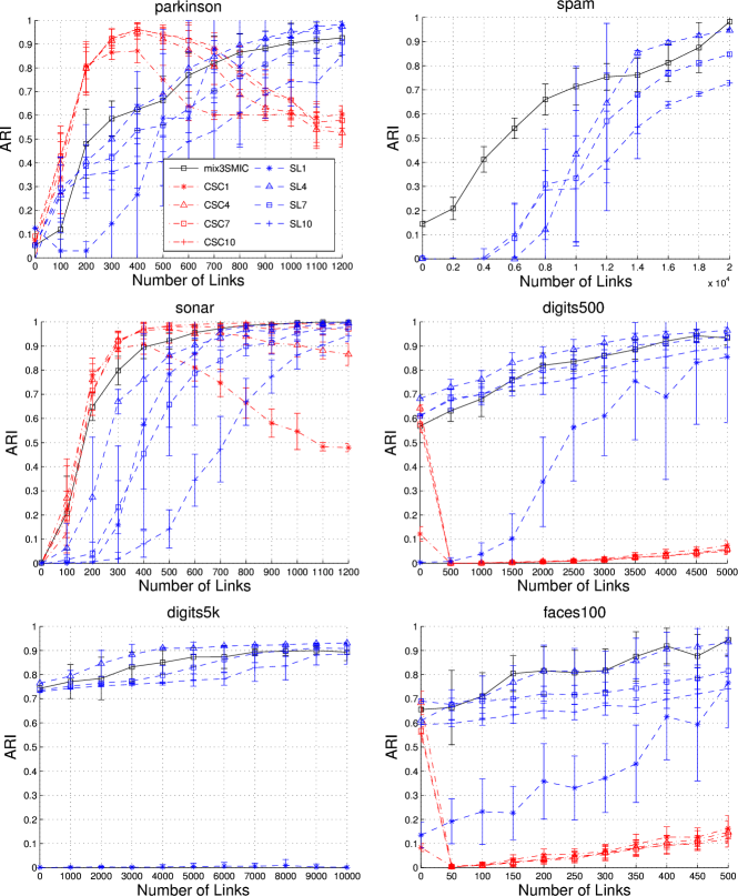
Figure 1: Experimental results.

We can separate the datasets into two groups. For digits500, digits5k, and faces100, the baseline performances without links are reasonable; the introduction of links significantly increase the performance, bringing it around $0.9$–$0.95$ from $0.5$–$0.8$.

For parkinson, spam, and sonar where the baseline performances without links are poor, introduction of links quickly allow the clustering algorithms to find better solutions. In particular, only 3% of links (relative to all possible pairs) was sufficient for parkinson to achieve reasonable performance and surprisingly only 0.1% for spam.

As shown in Figure 1, the performance of SL depends heavily on the choice of $t$, but there is no systematic way to choose $t$ for SL. It is important to notice that 3SMIC with $t$ chosen systematically based on Eq.(9) performs as good as SL with $t$ tuned optimally with hindsight. On the other hand, CSC performs rather stably for different values of $t$, and it works particularly well for binary problems with a small number of links. However, it performs very poorly for multi-class problems; we observed that the post k-means step is highly unreliable and poor local optimal solutions are often produced. For the binary problems, simply performing thresholding [17] instead of using k-means was found to be useful. However, there seems no simple alternatives in multi-class cases. The performance of CSC drops in parkinson and sonar when the number of links is increased, although such phenomena were not observed in SL and 3SMIC.

Overall, the proposed 3SMIC method was shown to be a promising semi-supervised clustering method.

5 Conclusions

In this paper, we proposed a novel information-maximization clustering method that can utilize side information provided as must-links and cannot-links. The proposed method, named semi-supervised SMI-based clustering (3SMIC), allows us to compute the clustering solution analytically. This is a strong advantage over conventional approaches such as constrained spectral clustering (CSC) that requires a post k-means step, because this post k-means step can be unreliable and cause significant performance degradation in practice. Furthermore, 3SMIC allows us to systematically determine tuning parameters such as the kernel width based on the information-maximization principle, given our reliance on the provided side information. Through experiments, we demonstrated that automatically-tuned 3SMIC perform as good as optimally-tuned spectral learning (SL) with hindsight.

The focus of our method in this paper was to inherit the analytical treatment of the original unsupervised SMIC in semi-supervised learning scenarios. Although this analytical treatment was demonstrated to be highly useful in experiments, our future work will explore more efficient use of must-links and cannot-links.

In the previous work [11], negative eigenvalues were found to contain useful information. Because must-link and cannot-link matrices can possess negative eigenvalues, it is interesting to investigate the role and effect of negative eigenvalues in the context of information-maximization clustering.

Appendix 0.A Least-Squares Mutual Information

The solution of SMIC depends on the choice of the kernel parameter included in the kernel function $K({\boldsymbol{x}},{\boldsymbol{x}}^{\prime})$. Since SMIC was developed in the framework of SMI maximization, it would be natural to determine the kernel parameter so as to maximize SMI. A direct approach is to use the SMI estimator $\widehat{\mathrm{SMI}}$ given by Eq.(6) also for kernel parameter choice. However, this direct approach is not favorable because $\widehat{\mathrm{SMI}}$ is an unsupervised SMI estimator (i.e., SMI is estimated only from unlabeled samples $\{{\boldsymbol{x}}_{i}\}_{i=1}^{n}$). On the other hand, in the model selection stage, we have already obtained labeled samples $\{({\boldsymbol{x}}_{i},y_{i})\}_{i=1}^{n}$, and thus supervised estimation of SMI is possible. For supervised SMI estimation, a non-parametric SMI estimator called least-squares mutual information (LSMI) [21] was proved to achieve the optimal convergence rate to the true SMI. Here we briefly review LSMI.

The key idea of LSMI is to learn the following density-ratio function [19],

$$r^{\ast}({\boldsymbol{x}},y):=\frac{p^{\ast}({\boldsymbol{x}},y)}{p^{\ast}({\boldsymbol{x}})p^{\ast}(y)},$$

without going through probability density/mass estimation of $p^{\ast}({\boldsymbol{x}},y)$, $p^{\ast}({\boldsymbol{x}})$, and $p^{\ast}(y)$. More specifically, let us employ the following density-ratio model:

$$r({\boldsymbol{x}},y;{\boldsymbol{\omega}}) :=\sum_{\ell:y_{\ell}=y}\omega_{\ell}L({\boldsymbol{x}},{\boldsymbol{x}}_{\ell}),$$ (10)

where ${\boldsymbol{\omega}}=(\omega_{1},\ldots,\omega_{n})^{\top}$ and $L({\boldsymbol{x}},{\boldsymbol{x}}^{\prime})$ is a kernel function. In practice, we use the Gaussian kernel

$$L({\boldsymbol{x}},{\boldsymbol{x}}^{\prime})=\exp\left(-\frac{\|{\boldsymbol{x}}-{\boldsymbol{x}}^{\prime}\|^{2}}{2\kappa^{2}}\right),$$

where the Gaussian width $\kappa$ is the kernel parameter. To save the computation cost, we limit the number of kernel bases to $500$ with randomly selected kernel centers.

The parameter ${\boldsymbol{\omega}}$ in the above density-ratio model is learned so that the following squared error is minimized:

$$\min_{\boldsymbol{\omega}}\frac{1}{2}\int\sum_{y=1}^{c}\Big{(}r({\boldsymbol{x}},y;{\boldsymbol{\omega}})-r^{\ast}({\boldsymbol{x}},y)\Big{)}^{2}p^{\ast}({\boldsymbol{x}})p^{\ast}(y)\mathrm{d}{\boldsymbol{x}}.$$ (11)

Let ${\boldsymbol{\omega}}^{(y)}$ be the parameter vector corresponding to the kernel bases $\{L({\boldsymbol{x}},{\boldsymbol{x}}_{\ell})\}_{\ell:y_{\ell}=y}$, i.e., ${\boldsymbol{\omega}}^{(y)}$ is the sub-vector of ${\boldsymbol{\omega}}=(\omega_{1},\ldots,\omega_{n})^{\top}$ consisting of indices $\{\ell\;|\;y_{\ell}=y\}$. Let $n_{y}$ be the number of samples in class $y$, which is the same as the dimensionality of ${\boldsymbol{\omega}}^{(y)}$. Then an empirical and regularized version of the optimization problem (11) is given for each $y$ as follows:

$$\min_{{\boldsymbol{\omega}}^{(y)}}\left[\frac{1}{2}{\boldsymbol{\omega}}^{(y)}{}^{\top}{\widehat{{\boldsymbol{H}}}}^{(y)}{\boldsymbol{\omega}}^{(y)}-{\boldsymbol{\omega}}^{(y)}{}^{\top}{\widehat{{\boldsymbol{h}}}}^{(y)}+\frac{\delta}{2}{\boldsymbol{\omega}}^{(y)}{}^{\top}{\boldsymbol{\omega}}^{(y)}\right],$$ (12)

where $\delta$ ($\geq 0$) is the regularization parameter. ${\widehat{{\boldsymbol{H}}}}^{(y)}$ is the $n_{y}\times n_{y}$ matrix and ${\widehat{{\boldsymbol{h}}}}^{(y)}$ is the $n_{y}$-dimensional vector defined as

$${\widehat{H}}_{\ell,\ell^{\prime}}^{(y)} :=\frac{n_{y}}{n^{2}}\sum_{i=1}^{n}L({\boldsymbol{x}}_{i},{\boldsymbol{x}}_{\ell}^{(y)})L({\boldsymbol{x}}_{i},{\boldsymbol{x}}_{\ell^{\prime}}^{(y)}),~{}~{}~{}{\widehat{h}}_{\ell}^{(y)}:=\frac{1}{n}\sum_{i:y_{i}=y}L({\boldsymbol{x}}_{i},{\boldsymbol{x}}_{\ell}^{(y)}),$$

where ${\boldsymbol{x}}^{(y)}_{\ell}$ is the $\ell$-th sample in class $y$ (which corresponds to ${\widehat{\omega}}^{(y)}_{\ell}$).

A notable advantage of LSMI is that the solution ${\widehat{{\boldsymbol{\omega}}}}^{(y)}$ can be computed analytically as

$${\widehat{{\boldsymbol{\omega}}}}^{(y)}=({\widehat{{\boldsymbol{H}}}}^{(y)}+\delta{\boldsymbol{I}})^{-1}{\widehat{{\boldsymbol{h}}}}^{(y)}.$$

Then a density-ratio estimator is obtained analytically as follows:

$$\widehat{r}({\boldsymbol{x}},y) =\sum_{\ell=1}^{n_{y}}{\widehat{\omega}}^{(y)}_{\ell}L({\boldsymbol{x}},{\boldsymbol{x}}^{(y)}_{\ell}).$$

The accuracy of the above least-squares density-ratio estimator depends on the choice of the kernel parameter $\kappa$ included in $L({\boldsymbol{x}},{\boldsymbol{x}}^{\prime})$ and the regularization parameter $\delta$ in Eq.(12). These tuning parameter values can be systematically optimized based on cross-validation as follows: First, the samples ${\mathcal{Z}}=\{({\boldsymbol{x}}_{i},y_{i})\}_{i=1}^{n}$ are divided into $M$ disjoint subsets $\{{\mathcal{Z}}_{m}\}_{m=1}^{M}$ of approximately the same size (we use $M=5$ in the experiments). Then a density-ratio estimator $\widehat{r}_{m}({\boldsymbol{x}},y)$ is obtained using ${\mathcal{Z}}\backslash{\mathcal{Z}}_{m}$ (i.e., all samples without ${\mathcal{Z}}_{m}$), and its out-of-sample error (which corresponds to Eq.(11) without irrelevant constant) for the hold-out samples ${\mathcal{Z}}_{m}$ is computed as

$$\mathrm{CV}_{m}:=\frac{1}{2|{\mathcal{Z}}_{m}|^{2}}\sum_{{\boldsymbol{x}},y\in{\mathcal{Z}}_{m}}\widehat{r}_{m}({\boldsymbol{x}},y)^{2}-\frac{1}{|{\mathcal{Z}}_{m}|}\sum_{({\boldsymbol{x}},y)\in{\mathcal{Z}}_{m}}\widehat{r}_{m}({\boldsymbol{x}},y),$$

where $\sum_{{\boldsymbol{x}},y\in{\mathcal{Z}}_{m}}$ denotes the summation over all combinations of ${\boldsymbol{x}}$ and $y$ in ${\mathcal{Z}}_{m}$ (and thus $|{\mathcal{Z}}_{m}|^{2}$ terms), while $\sum_{({\boldsymbol{x}},y)\in{\mathcal{Z}}_{m}}$ denotes the summation over all pairs $({\boldsymbol{x}},y)$ in ${\mathcal{Z}}_{m}$ (and thus $|{\mathcal{Z}}_{m}|$ terms). This procedure is repeated for $m=1,\ldots,M$, and the average of the above hold-out error over all $m$ is computed as

$$\mathrm{CV}:=\frac{1}{M}\sum_{m=1}^{M}\mathrm{CV}_{m}.$$

Then the kernel parameter $\kappa$ and the regularization parameter $\delta$ that minimize the average hold-out error $\mathrm{CV}$ are chosen as the most suitable ones.

Finally, given that SMI (2) can be expressed as

$$\mathrm{SMI} =-\frac{1}{2}\int\sum_{y=1}^{c}r^{\ast}({\boldsymbol{x}},y)^{2}p^{\ast}({\boldsymbol{x}})p^{\ast}(y)\mathrm{d}{\boldsymbol{x}}+\int\sum_{y=1}^{c}r^{\ast}({\boldsymbol{x}},y)p^{\ast}({\boldsymbol{x}},y)\mathrm{d}{\boldsymbol{x}}-\frac{1}{2},$$

an SMI estimator based on the above density-ratio estimator, called least-squares mutual information (LSMI), is given as follows:

$$\mathrm{LSMI}:=-\frac{1}{2n^{2}}\sum_{i,j=1}^{n}\widehat{r}({\boldsymbol{x}}_{i},y_{j})^{2}+\frac{1}{n}\sum_{i=1}^{n}\widehat{r}({\boldsymbol{x}}_{i},y_{i})-\frac{1}{2},$$

where $\widehat{r}({\boldsymbol{x}},y)$ is a density-ratio estimator obtained above.

References

- Agakov and Barber [2006] F. Agakov and D. Barber. Kernelized infomax clustering. In Y. Weiss, B. Schölkopf, and J. Platt, editors, Advances in Neural Information Processing Systems 18, pages 17–24, Cambridge, MA, USA, 2006. MIT Press.
- Ali and Silvey [1966] S. M. Ali and S. D. Silvey. A general class of coefficients of divergence of one distribution from another. Journal of the Royal Statistical Society, Series B, 28(1):131–142, 1966.
- Basu et al. [1998] A. Basu, I. R. Harris, N. L. Hjort, and M. C. Jones. Robust and efficient estimation by minimising a density power divergence. Biometrika, 85(3):549–559, 1998.
- Csiszár [1967] I. Csiszár. Information-type measures of difference of probability distributions and indirect observation. Studia Scientiarum Mathematicarum Hungarica, 2:229–318, 1967.
- Girolami [2002] M. Girolami. Mercer kernel-based clustering in feature space. IEEE Transactions on Neural Networks, 13(3):780–784, 2002.
- Goldberg [2007] A. B. Goldberg. Dissimilarity in graph-based semi-supervised classification. In Proceedings of the Eleventh International Conference on Artificial Intelligence and Statistics (AISTATS2007), pages 155–162, 2007.
- Gomes et al. [2010] R. Gomes, A. Krause, and P. Perona. Discriminative clustering by regularized information maximization. In J. Lafferty, C. K. I. Williams, R. Zemel, J. Shawe-Taylor, and A. Culotta, editors, Advances in Neural Information Processing Systems 23, pages 766–774, 2010.
- Hubert and Arabie [1985] L. Hubert and P. Arabie. Comparing partitions. Journal of Classification, 2(1):193–218, 1985.
- Kamvar et al. [2003] S. D. Kamvar, D. Klein, and C. D. Manning. Spectral learning. In Proceedings of the 18th International Joint Conference on Artificial Intelligence (IJCAI2003), pages 561–566, 2003.
- Kullback and Leibler [1951] S. Kullback and R. A. Leibler. On information and sufficiency. The Annals of Mathematical Statistics, 22:79–86, 1951.
- Laub and Müller [2004] J. Laub and K.-R. Müller. Feature discovery in non-metric pairwise data. Journal of Machine Learning Research, 5:801–818, Jul. 2004.
- MacQueen [1967] J. B. MacQueen. Some methods for classification and analysis of multivariate observations. In Proceedings of the 5th Berkeley Symposium on Mathematical Statistics and Probability, volume 1, pages 281–297, Berkeley, CA, USA, 1967. University of California Press.
- Ng et al. [2002] A. Y. Ng, M. I. Jordan, and Y. Weiss. On spectral clustering: Analysis and an algorithm. In T. G. Dietterich, S. Becker, and Z. Ghahramani, editors, Advances in Neural Information Processing Systems 14, pages 849–856, Cambridge, MA, USA, 2002. MIT Press.
- Pearson [1900] K. Pearson. On the criterion that a given system of deviations from the probable in the case of a correlated system of variables is such that it can be reasonably supposed to have arisen from random sampling. Philosophical Magazine Series 5, 50(302):157–175, 1900.
- Schölkopf and Smola [2002] B. Schölkopf and A. J. Smola. Learning with Kernels. MIT Press, Cambridge, MA, USA, 2002.
- Shannon [1948] C. Shannon. A mathematical theory of communication. Bell Systems Technical Journal, 27:379–423, 1948.
- Shi and Malik [2000] J. Shi and J. Malik. Normalized cuts and image segmentation. IEEE Transactions on Pattern Analysis and Machine Intelligence, 22(8):888–905, 2000.
- Sugiyama et al. [2011] M. Sugiyama, M. Yamada, M. Kimura, and H. Hachiya. On information-maximization clustering: Tuning parameter selection and analytic solution. In L. Getoor and T. Scheffer, editors, Proceedings of 28th International Conference on Machine Learning (ICML2011), pages 65–72, Bellevue, Washington, USA, Jun. 28–Jul. 2 2011.
- Sugiyama et al. [2012] M. Sugiyama, T. Suzuki, and T. Kanamori. Density Ratio Estimation in Machine Learning. Cambridge University Press, Cambridge, UK, 2012.
- Suzuki and Sugiyama [2013] T. Suzuki and M. Sugiyama. Sufficient dimension reduction via squared-loss mutual information estimation. Neural Computation, 3(25):725–758, 2013.
- Suzuki et al. [2009] T. Suzuki, M. Sugiyama, T. Kanamori, and J. Sese. Mutual information estimation reveals global associations between stimuli and biological processes. BMC Bioinformatics, 10(1):S52 (12 pages), 2009.
- Wagstaff and Cardie [2000] K. Wagstaff and C. Cardie. Clustering with instance-level constraints. In Proceedings of the Seventeenth International Conference on Machine Learning (ICML2000), pages 1103–1110, 2000.
- Wagstaff et al. [2001] K. Wagstaff, C. Cardie, S. Rogers, and S. Schrödl. Constrained k-means clustering with background knowledge. In Proceedings of the Eighteenth International Conference on Machine Learning (ICML2001), pages 577–584, 2001.
- Wang and Davidson [2010] X. Wang and I. Davidson. Flexible constrained spectral clustering. In Proceedings of the 16th ACM SIGKDD International Conference on Knowledge Discovery and Data Mining (KDD2010), pages 563–572, 2010.
- Zelnik-Manor and Perona [2005] L. Zelnik-Manor and P. Perona. Self-tuning spectral clustering. In L. K. Saul, Y. Weiss, and L. Bottou, editors, Advances in Neural Information Processing Systems 17, pages 1601–1608, Cambridge, MA, USA, 2005. MIT Press.