The Blazar Emission Environment:
Insight from Soft X-ray Absorption

Abstract

Collecting experimental insight into the relativistic particle populations and emission mechanisms at work within TeV-emitting blazar jets, which are spatially unresolvable in most bands and have strong beaming factors, is a daunting task. New observational information has the potential to lead to major strides in understanding the acceleration site parameters. Detection of molecular carbon monoxide (CO) in TeV emitting blazars, however, implies the existence of intrinsic gas, a connection often found in photo-dissociated region models and numerical simulations. The existence of intrinsic gas within a blazar could provide a target photon field for Compton up-scattering of photons to TeV energies by relativistic particles. We investigate the possible existence of intrinsic gas within the three TeV emitting blazars RGB J0710+591, W Comae and 1ES 1959+650 which have measurements or upper limits on molecular CO line luminosity using an independent technique which is based on the spectral analysis of soft X-rays. Evidence for X-ray absorption by additional gas beyond that measured within the Milky Way is searched for in Swift X-ray Telescope (XRT) data between 0.3 and 10 keV. Without complementary information from another measurement, additional absorption could be misinterpreted as an intrinsically curved X-ray spectrum since both models can frequently fit the soft X-ray data. After breaking this degeneracy, we do not find evidence for intrinsically curved spectra for any of the three blazars. Moreover, no evidence for intrinsic gas is evident for RGB J0710+591 and W Comae, while the 1ES 1959+650 XRT data support the existence of intrinsic gas with a column density of $\sim$1$\times 10^{21}$cm^-2.

1 Introduction

Within the canonical classification of active galactic nuclei (AGN), blazars are a type of active galaxy with a relativistic jet pointed toward the observer. These galaxies harbor relativistic particle populations with intrinsic emission characteristics which largely remain difficult to characterize. Blazars produce a non-thermal spectral energy distribution (SED), characterized by two broad peaks in the $\nu$F_ν representation. The source of the lower-energy peak can be attributed to the synchrotron radiation of relativistic leptons in the presence of a magnetic field. The mechanism responsible for this relativistic population of leptons (e. g. diffusive parallel shock acceleration, oblique shock acceleration or magnetic reconnection driven flows) remains an open question.

The origin of the higher-energy SED peak has been attributed to inverse-Compton up-scattering by the relativistic jet leptons of either the synchrotron photons themselves, namely synchrotron self-Compton (SSC) emission, or a photon field external to the jet, namely external Compton (EC) emission (e. g. Dermer et al. (1992); Maraschi et al. (1992)). This external field of photons could arise from emission from a dusty torus, broad line region or some other source within the blazar. The key feature that distinguishes EC emission from SSC emission, therefore, is the presence of additional gas that can supply an external photon field. Alternative models attribute the higher energy peak to hadron acceleration leading to proton synchrotron emission and/or pion production accompanied by resulting cascade emission (e. g. Aharonian et al. (2002); Bednarek (1993); Mücke et al. (2003); Dermer et al. (2012)).

Blazars are sub-classified as flat-spectrum radio-loud quasars if broad emission lines are visible or, otherwise, as BL Lac objects. BL Lac objects are sub-categorized based on the frequency location of the lower-energy peak, with low-synchrotron-peaked (LSP) BL Lac objects having a peak below $10^{14}$ Hz, intermediate-synchrotron-peaked (ISP) BL Lac objects peaking between $10^{14}$ and $10^{15}$ Hz and high-synchrotron-peaked (HSP) BL Lac objects showing a peak above $10^{15}$ Hz (Abdo et al., 2010a). Across these different sub-classes, blazars exhibit a continuous variation in their SED. This has been interpreted as an evolutionary sequence associated with the variation of the diffuse radiation field in the surroundings of the relativistic jet (Fossati et al., 1998; Böttcher & Chiang, 2002; Ghisellini & Tavecchio, 2008). Under this paradigm, LSP blazars are expected to have an appreciable external radiation field which facilitates effective cooling and favors a EC broadband representation while HSPs lack a source of external radiation and would be described with an SSC emission scenario.

Measurements which can probe for the existence of intrinsic gas which might produce an external radiation field for Compton up-scattering, however, are challenging for BL Lac objects . The bright, non-thermal continuum emitted by the blazar jet makes the discrimination between SSC and EC emission mechanisms difficult. Broadband modeling of BL Lacs is a common method for the investigation of the non-thermal emission mechanism at work within a blazar jet (e. g. Tramacere et al. (2011); Aleksić et al. (2012); Abramowski et al. (2012)). These models utilize various input parameters which describe the non-thermal emission, including the particle injection parameter, $q$, which also represents the index of the relativistic electron energy distribution in the absence of significant cooling processes which can deform the power-law emission. The relativistic particles are directly responsible for the synchrotron emission which makes up the lower energy SED peak. Since the spectrum of synchrotron radiation follows from the energy distribution of the emitting particles, the highest energy particles can be directly probed through X-ray observations. More specifically, the observed radiation spectrum can be translated into the spectrum of relativistic particles emitting that synchrotron radiation.

Two functional forms are commonly adopted to describe the observed synchrotron spectrum: a power-law model and a log-parabolic model. A power-law synchrotron spectrum with photon index $\alpha$ originates from a particle power-law energy spectrum with index $q=2\alpha+1$ (Rybicki & Lightman, 1979), where $q$ is equal to the index of the input particle distribution in the absence of a cooled high energy tail. Similarly, a log-parabolic radiation spectrum can be produced by a log-parabolic distribution of relativistic particles (Paggi et al., 2009) and can be interpreted as evidence for a statistical acceleration process (Tramacere et al., 2007; Massaro et al., 2006, 2004; Costamante, 2001; Tagliaferri et al., 2003, e.g.). This log-parabolic emission can also be interpreted as representing a power-law particle distribution with a cooled high energy tail, producing an intrinsically curved X-ray spectrum. An accurate determination of the spectral shape of the underlying population is key in the elucidation of the relativistic acceleration mechanism at work within a blazar jet. Fundamentally different acceleration methods produce varying particle spectra, and intrinsic spectral curvature is a possible signature of statistical acceleration.

Regardless of the intrinsic spectral shape of the synchrotron emission, the non-thermal X-ray radiation from any extragalactic X-ray emitter undergoes absorption by the interstellar medium of our own Galaxy. The effective energy-dependent cross section results from the absorption of photons by intervening elements such as (but not limited to) C, N and O, an effect extending up to 10 keV. These absorption cross sections have been calculated per neutral hydrogen column density (N_HI) as a function of energy in the 0.03-10 keV range (Morrison & McCammon, 1983) and can be used to estimate the amount of absorption extragalactic X-ray emission undergoes because of the intervening gas within the Milky Way.

Both an absorbed power law and an absorbed log parabola have been shown to produce acceptable fits to blazar spectral data between 0.3 and 10 keV. The hydrogen column density that is used to scale the abundance of the additional absorbing elements is typically fixed to the Galactic value as measured by the LAB survey (Kalberla et al., 2005). In practice, these fits do not allow for the presence of additional gas in the blazar host galaxy. There have, however, been a limited number of blazars which, when fit with an absorbed power-law model with a free column density, show a fitted value in excess to that measured in the Milky Way (e. g. Aliu et al. (2011, 2012)). However, some ambiguity in the interpretation of the data remain. For these instances, the use of an absorbed log-parabolic model with a fixed Galactic N_HI column density allows for an intrinsically curved spectrum and can provide an improved fit to the X-ray data without requiring additional absorption within the blazar emission region.

We argue that an apparently curved spectrum observed in TeV BL Lacertae objects may, in some cases, be partially or entirely due to intrinsic blazar column density beyond that measured within our own Galaxy, similarly to what was found in Tavecchio et al. (2002) for a flat-spectrum radio quasar. Detection of additional X-ray absorption exceeding that expected from the Milky Way, therefore, might provide an experimental probe of the emission mechanism at work within TeV blazars (e. g. SSC or EC emission). To investigate the degeneracy between intrinsic curvature in the X-ray spectrum and additional absorption from gas in the blazar host galaxy, we utilize independent observations of the gas content in the surroundings of the blazars.

Recent millimetric observations of CO have probed the molecular gas content in three TeV-emitting blazars (Fumagalli et al., 2012). A common result of photo-dissociation region (PDR) models and numerical simulations is that CO molecules form in regions where the UV radiation has been shielded by gas and dust, (e. g. Tielenn & Hollenbach (1985); Krumholz et al. (2009); Glover & Clark (2012)). The detection of molecular gas in a galaxy is therefore a signpost of additional intervening material in the surroundings of the blazar, similar to the interstellar gas that absorbs soft X-rays within our own Galaxy. While the exact conversion between the observed CO column density and the hydrogen column density (both in atomic and molecular phase) would require a detailed knowledge of the chemical and physical state of the gas as well as of the impinging radiation field, it is reasonable to expect that the presence of CO is associated with a hydrogen column density $>$10 M_⊙pc^-2 ($\sim 1\times 10^{21}$cm^-2). Similarly, in normal conditions it would be surprising to find regions in which the N_HI column density greatly exceeds 10 M_⊙pc^-2 without a molecular phase.

Millimetric observations that are sufficiently deep to map CO in blazars have thus far only been completed for three sources, namely RGB J0710+591, W Comae and 1ES 1959+650. With the understanding that a sample of three blazars is far too limited to draw general conclusions, we investigate the relation between the presence of molecular gas and evidence for intrinsic column density in blazars as well as intrinsic X-ray spectral curvature, as inferred from spectral fitting.

In this work we show that the possibility of combining independent diagnostics at different frequencies has immediate implications for the physical interpretation of emission processes at work within TeV-emitting blazar jets. In Section 2 we discuss the Swift XRT observations and data reduction which allow for the investigation of additional absorption by intrinsic gas. In Section 3 we summarize the results of the spectral analysis for each source, addressing the possibility for both intrinsic absorption and spectral curvature. Finally, we discuss our results in a broader context with regard to blazar non-thermal emission and the implications for the blazar evolutionary theory.

2 Observations and Data Reduction

The data set includes all Swift X-ray Telescope (XRT) exposures of RGB J0710+591, W Comae, and 1ES 1959+650 since the launch of the instrument in November 2004 (Gehrels et al., 2004). The summary of each exposure used can be found in Tables 1-4. The XRT is a grazing incidence Wolter-I telescope which focuses X-rays between 0.2 and 10 keV onto a 100 cm² CCD (Burrows et al., 2005). The data were analyzed using the HEASoft package v6.12. Event files were cleaned and calibrated with standard criteria with the xrtpipeline task, using only events between 0.3 and 10 keV having a grade 0-12 for windowed timing (wt) mode and 0-2 for photon counting (pc) mode. Additionally, events having energy between 0.4 and 0.7 keV were removed from the analysis due to the effects of the oxygen edge at 0.54 keV. More details on the Swift XRT effective area can be found in Evans et al. (2009).

For windowed timing mode, rectangular source regions with length and width of 45 and 8 pixels were used for spectral analysis. Background regions were extracted from similarly sized rectangular regions of nearby source-free sky, aligned along the windowed timing one dimensional stream in sky coordinates.

For photon counting mode, circular source regions of radius 20 pixels and centered on the source were used along with similarly sized background regions of nearby source-free sky. If a source showed a count rate greater than 0.5 counts per sec, pileup was accounted for by using an annular source region with inner radius of 2 pixels and outer radius 20 pixels to remove the pile-up contamination in the inner part of the point spread function. For 1ES 1959+650, a source showing consistently high count rates between 3 and 12 counts per second, we only include windowed timing exposures lasting more than 0.5 ks.

The response matrices available from CALDB were used to create ancillary response files with xrtmkarf. For single observations with sufficient statistics to allow spectral fitting, source spectra were binned to require 30 counts per bin. Single exposures providing count levels too low to allow for the bin minimum required for accurate $\chi^{2}$ minimization fitting were first summed with xselect, with the exposure files summed with ximage, before being binned to require 30 counts per bin. This summation was only necessary for the low count levels found for W Comae. Summing all photon counting mode exposures of W Comae provided 176 bins with more than 30 counts. It is noted that the summation of these exposures introduced a possibility for summing different spectral states.

3 Spectral Analysis and Results

The spectral analysis was performed with XSPEC Version 12.7.1 and a suite of in-house IDL routines. We fit the data with two spectral models. The first is an absorbed power-law model (wabs(powerlaw) in XSPEC), with an additional exponent to represent additional neutral hydrogen column density beyond the Milky Way

$$F(E)_{PL}=Ke^{-(N^{\rm MW}_{\rm HI}+N^{\rm INT}_{\rm HI})\sigma(E)}(E)^{-\alpha},$$ (1)

referred to as the PL model for the remainder of this work, where $\alpha$ is the spectral slope, K is the normalization parameter and $\sigma(E)$ is the non-Thompson energy dependent photoelectric cross section from Morrison & McCammon (1983). N${}^{\rm MW}_{\rm HI}$ is the neutral hydrogen column density within the Milky Way, as measured by the LAB survey. The LAB-measured neutral hydrogen densities for each blazar are 4.16$\times 10^{20}$cm^-2, 1.97$\times 10^{20}$cm^-2 and 1.00$\times 10^{21}$cm^-2 for RGB J0710+591, W Comae and 1ES 1959+650, respectively. N${}^{\rm INT}_{\rm HI}$ is the blazar neutral hydrogen column density, both in units of cm^-2. We note that this analysis does not allow differentiation between blazar-intrinsic and intervening gas residing along the line of sight to the blazar. With the possibility for galaxy clustering, the local environment around the blazars may contain an overdensity of galaxies that can contribute to the observed absorption. Any additional column density found through this analysis is assumed to be in the vicinity of the blazar.

The LAB survey consists of observations of 21-cm emission from Galactic neutral hydrogen over the entire sky. The LAB Survey is a sensitive Milky Way neutral hydrogen survey, with extensive coverage both spatially and kinematically. The survey merges the Leiden/Dwingeloo Survey (LDS: Hartmann & Burton (1997)) of the sky north of $-30$ degrees declination with the Instituto Argentino de Radioastronom a Survey (IAR: Arnal et al. (2000); Bajaja et al. (2005)) of the sky south of $-25$ degrees declination. Uncertainties in N${}^{\rm MW}_{\rm HI}$ column densities, as reported by the LAB survey, are between 2 and 3%, with $\sim$1% from scale uncertainty and $\sim$ 1% from uncertainties in the correction for stray radiation.

The second spectral model applied to the data is an absorbed log-parabola (wabs(logpar) in XSPEC) with an additional exponent to represent additional neutral hydrogen column density beyond the Milky Way, referred to as the LP model for the remainder of this work. This model has been suggested to better represent TeV-detected blazar X-ray spectra (e. g. Massaro et al. (2008); Tramacere et al. (2007)). This model allows the spectral index to vary as a function of energy, according to the equation

$$F(E)_{LP}=Ke^{-(N^{\rm MW}_{\rm HI}+N^{\rm INT}_{\rm HI})\sigma(E)}(E)^{-(\alpha+\beta{\rm log}(E))},$$ (2)

with a normalization factor K, photoelectric cross section and hydrogen column densities similar to those described for the PL model above.

These models were fit to the XRT data of the three blazars with both N${}^{\rm INT}_{\rm HI}$ set to zero and with N${}^{\rm INT}_{\rm HI}$ allowed to vary, while requiring it to remain equal to or greater than zero. The best fits for each of the models are shown in Figure 1 for each of the blazars. These fits are completed for the Observation ID 0003156006 for RGB J0710+591, the summed exposure of W Comae and Observation ID 00035025004 for 1ES 1959+650. For RGB J 0710+591 and 1ES 1959+650, the fits are shown for the exposure with the highest statistics and are meant to be representative of the fitting results. The fitted parameters from Figure 1 are shown in bold in Tables 1, 3 and 4.

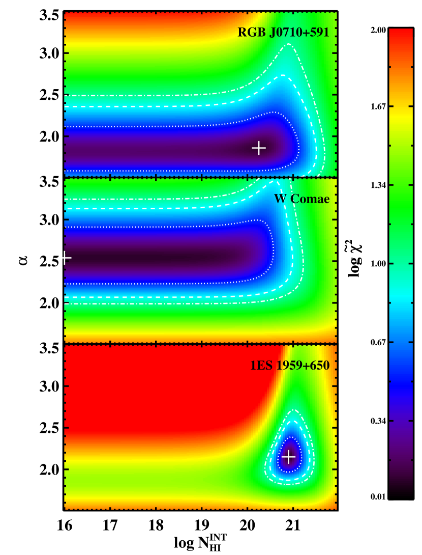
Figure 2: The reduced $\chi^{2}$ contours for the PL model for the RGB J0710+591 Observation 0003156006, the W Comae summed exposure, and the 1ES 1959+650 Observation 00035025004. The white dotted, dashed and dash-dotted lines represent the one, two and three sigma confidence contours on the joint distribution of parameters. The N${}^{\rm INT}_{\rm HI}$ parameter for RGB J0710+591 and W Comae (top and middle panels) are shown to be unconstrained, showing that the data do not favor any additional absorption from intrinsic gas within the blazar and beyond that of the Milky Way. The minimum of the fit for RGB J0710+591, however, lies within the defined parameter space, while it does not for the summed W Comae data.

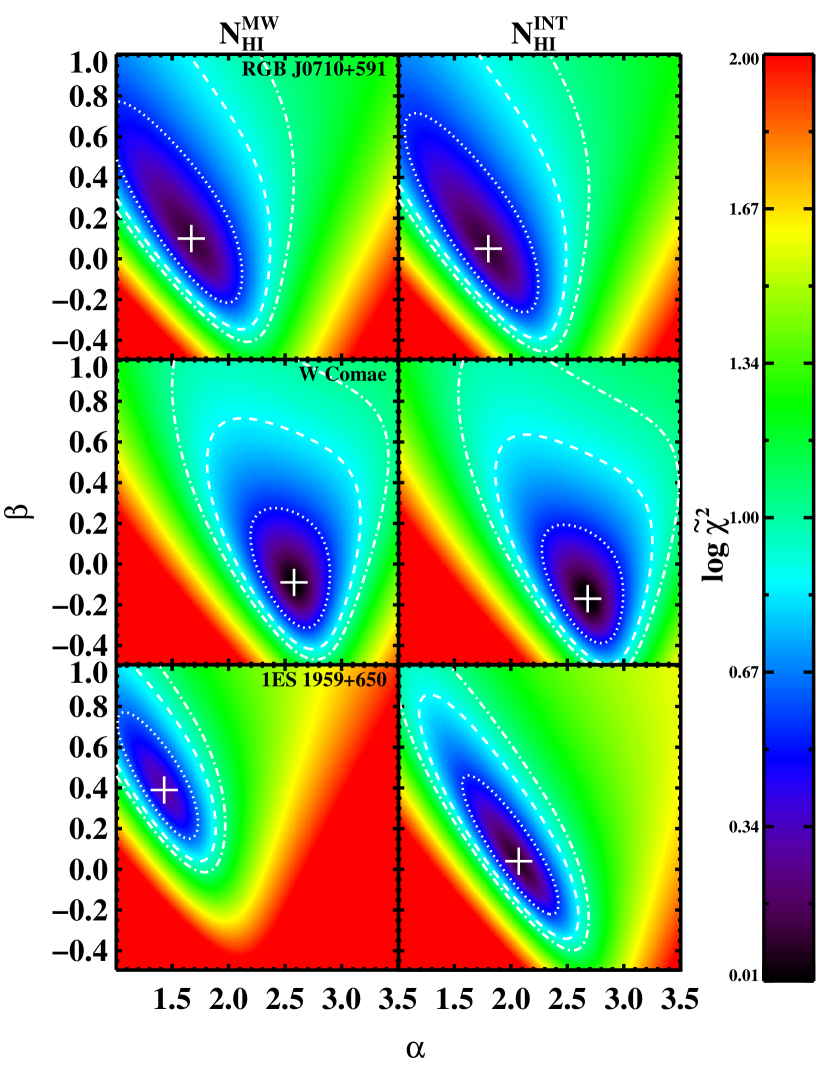
Figure 3: Reduced $\chi^{2}$ contours for the LP model for the RGB J0710+591 Observation 0003156006, the W Comae summed exposure and the 1ES 1959+650 Observation 00035025004 for N${}^{\rm INT}_{\rm HI}$ lacking (left) and inclusive (right) column density fits. The contours are similarly represented, as described in Figure 2. The index $\alpha$ and curvature $\beta$ parameters are not seen to significantly change for free and fixed N_HI fits for RGB J0710+591 and W Comae. For 1ES 1959+650, the $\alpha$ and $\beta$ parameters change from 1.5 and 0.4 to 2.1 and 0, respectively, when N${}^{\rm INT}_{\rm HI}$ is included in the fit. This change suggests that if N${}^{\rm INT}_{\rm HI}$ column density is included, no intrinsic curvature in the spectrum of 1ES 1959+650 is necessary to match the observed spectrum. Note that the x- and y-axes are interchanged in these plots compared to Figure 2.

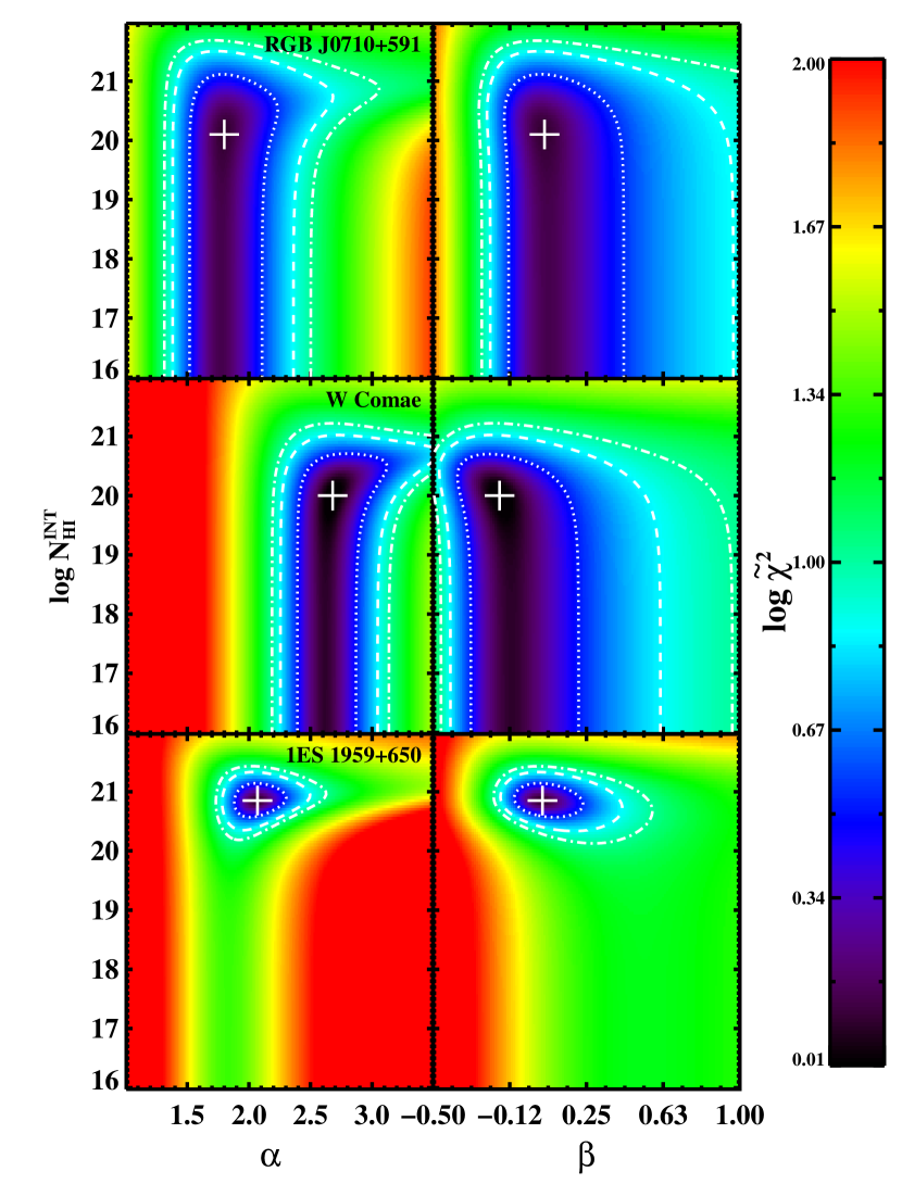
Figure 4: Reduced $\chi^{2}$ contours for the LP model for the RGB J0710+591 Observation 0003156006, the W Comae summed exposure and the 1ES 1959+650 Observation 00035025004 for fitted N${}^{\rm INT}_{\rm HI}$ column density. The contours are similarly represented, as described in Figure 2. The column densities of RGB J0710+591 and W Comae are seen to be unconstrained, while they are well defined for 1ES 1959+650, showing an intrinsic column density of order 1$\times 10^{21}$cm^-2, in addition to the 1$\times 10^{21}$cm^-2 as measured by the LAB Galactic N_HI survey.

The parameter spaces for the spectral models as applied to the data are illustrated by reduced $\chi^{2}$ contours in Figures 2-4. The N${}^{\rm INT}_{\rm HI}$ column density is allowed to vary when producing these contours, except for left hand column of Figure 3, when illustrating the fitted $\alpha$ and $\beta$ parameters resulting for the LP model with and without a N${}^{\rm INT}_{\rm HI}$ column density. These contours show parameter constraints (or lack thereof) during the spectral $\chi^{2}$ fitting procedures. The white dotted, dashed and dash-dotted lines represent the one, two and three sigma confidence contours on the joint distribution of parameters.

3.1 RGB J0710+591

The spectral models were applied to each of the 13 Swift XRT observations of RGB J0710+591 and are summarized in Table 1. When fit with both PL and LP models which allow for N${}^{\rm INT}_{\rm HI}$ column density, there is no significant evidence for the existence of additional gas, e. g. N${}^{\rm INT}_{\rm HI}$ parameters are consistent with zero. These fits provide parameter values equivalent to the N${}^{\rm INT}_{\rm HI}$-lacking fits. Due to this redundancy, the resulting parameters are only quoted for fits where N${}^{\rm INT}_{\rm HI}$ is not included. The exposures provide comparable fit qualities for the N${}^{\rm MW}_{\rm HI}$ only and N${}^{\rm INT}_{\rm HI}$ inclusive models.

As shown in Figure 3 for the LP model, the fitted $\alpha$ and $\beta$ parameters do not change significantly when allowing for a non-zero N${}^{\rm INT}_{\rm HI}$ column density. Additionally, the lack of constraint on the N${}^{\rm INT}_{\rm HI}$ column density with respect to these parameters is evident in the top panel of Figure 4. When fitting the data with a LP model, negligible curvature ($\beta$) is found for a majority of the observations. This $\beta\sim 0$ result indicates that the PL model is sufficient to describe the X-ray emission from this blazar.

There are a few instances where significant negative curvature is found from the LP fitting. This unexpected result is likely due to covariance between the $\alpha$ and $\beta$ parameters ( i. e. moving diagonally in the Figure 3 parameter spaces). One can see that in each instance where a negative curvature parameter is found, the fitted index $\alpha$ softens to values of $\sim$2 or less. Due to the unlikely possibility to produce a concave distribution of relativistic particles by traditional acceleration mechanisms, a more physical result might be found by fitting a log-parabolic model with $\beta>0$ limitations.

3.2 W Comae

The PL and LP spectral models were applied to the summed photon counting mode exposures of W Comae. The 73 observations summed to 1.3$\times 10^{5}$ seconds and are summarized in Table 2, with the fitting results in Table 3. As illustrated by the confidence contours in the middle panels of Figures 2 and 4, application of the PL and LP models which allow for non-zero N${}^{\rm INT}_{\rm HI}$ column density result in N${}^{\rm INT}_{\rm HI}$ parameters consistent with zero, showing no significant evidence for an intervening gas within the blazar and providing parameter values equivalent to the fixed N${}^{\rm MW}_{\rm HI}$ fits.

Similarly to the LP model result for RGB J0710+591, the fitted $\alpha$ and $\beta$ parameters do not change significantly when including N${}^{\rm INT}_{\rm HI}$. The negative curvature parameter $\beta$ found when applying the LP model to the summed W Comae spectra may indicate a correlation in the $\alpha$ and $\beta$ parameters, similarly as the trend presented in the RGB J0710+591 data. This specific case of negative curvature might also be a result of summing multiple exposures. Investigation of spectral effects due to summing were completed by fitting the summed exposure while ignoring bins between 1.5 and 2.2 keV in order to remove possible pollution from the Si K$\alpha$ edge. Removing these bins, however, did not change the spectral results.

Spectral effects introduced through the summation of different spectral states and/or flux levels may also introduce distorted spectral features such as concavity (i.e. the summation of a bright soft state with a low hard state). The previously observed broadband variability of blazars at all wavebands and timescales probed supports this possibility. X-ray spectral variability of W Comae during a flare, however, shows the source to harden during periods of elevated flux (Acciari et al., 2009). We take this behavior as evidence that the concavity of the summed spectrum is not likely due to the summation of bright soft and low hard states. The 73 observations show the count rate of W Comae to vary between 0.05 and 3.8 counts per second. Details of X-ray variability of BL Lac objects are described in Böttcher & Chiang (2002).

If the resulting $\chi^{2}$ values are used at face value to determine which model best represents W Comae, one would conclude that the curved LP model is the most appropriate. However, the convex curvature of the radiation spectrum is not easily described by standard acceleration mechanisms and so we favor a PL model over a LP model for W Comae.

3.3 1ES 1959+650

When fitting both the PL and LP models to 1ES 1959+650, a significant N${}^{\rm INT}_{\rm HI}$ column density is derived (see Tables 3 and 4 for a summary of all results). The $\alpha$ and $\beta$ parameter for the LP model can be seen to change significantly when N${}^{\rm INT}_{\rm HI}$ is included in the fit (Figure 3). The $\beta$ parameter becomes consistent with zero when N${}^{\rm INT}_{\rm HI}$ is included in the fit, indicating that if the possibility for intrinsic gas in the blazar emission environment is allowed, the particle population can be represented with an uncurved power-law spectrum. Evidence for additional absorption exceeding that by the Milky Way was also found for power-law fits of XMM X-ray observations of 1ES 1959+650 in Perlman et al. (2005), although the additional column density was interpreted as evidence for a curved log-parabolic spectrum.

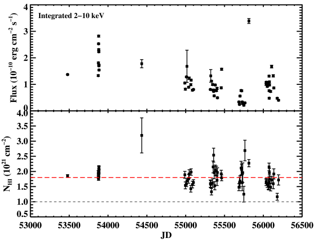
Figure 5: A light curve of the 2$-$10 keV flux and fitted N${}^{\rm INT}_{\rm HI}$ column density for the 61 windowed timing observations of 1ES 1959+650. The flux is seen to vary widely, with a fit to a constant resulting in a $\chi^{2}$ of 35089 for 61 degrees of freedom. The N${}^{\rm INT}_{\rm HI}$ column density is also variable, but shows a smaller $\chi^{2}$ value of 320 when fit with a constant, with an average of 0.8$\times 10^{21}$cm^-2 (denoted by the red dashed line), nearly equal to the value N${}^{\rm MW}_{\rm HI}$ of 1.0$\times 10^{21}$cm^-2 as reported by the LAB survey (denoted by the grey dotted line). This additional 0.8$\times 10^{21}$cm^-2 column density beyond that of the LAB value is in significant excess of the 1-2% error reported for the LAB survey measurements. The slight variability of the N${}^{\rm INT}_{\rm HI}$ column density is not immediately expected and, if real, suggests that the column density is very close to the non-thermal emission region. However, the errors shown here do not account for slight correlations between other fitted PL parameters.

The variation of the PL-fitted blazar column density between observations is illustrated in the light curve in Figure 5, showing the PL N${}^{\rm INT}_{\rm HI}$ column densities in comparison to the large flux variations exhibited by the blazar ($\chi^{2}=35089$ for 61 degrees of freedom). The N${}^{\rm INT}_{\rm HI}$ values are less variable ($\chi^{2}=320$ for 61 degrees of freedom) with an average of 8$\times 10^{20}$cm^-2, nearly equal to the Galactic contribution of 1.0$\times 10^{21}$cm^-2, as measured by the LAB survey. If the variability of the column density is real, it would suggest that the gas is local to the non-thermal emission region. X-ray variability of AGN is commonly observed (e.g. Mushotzky et al. (1993); Vagnetti et al. (2011)) and has been attributed to the variation of intrinsic absorption and covering fraction of the galaxy (Abrassart & Czerny, 2000; Wachter et al., 1988). As a geometrically selected subtype of jetted AGN, variability of column density within a blazar is possible. However, the variability of column density for 1ES 1959+650 shown in Figure 5 might result from the underestimation of the N${}^{\rm INT}_{\rm HI}$ errors as they do not account for correlations between fitting parameters.

4 Discussion and Conclusion

The 0.3-10 keV spectral analysis of the three blazars which have molecular CO line luminosity measurements and upper limits support a possible connection between blazar CO line luminosity and hydrogen column density, providing a possible method to directly probe the relativistic particle energy distribution. The two sources RGB J0710+591 and W Comae, both of which are shown to exhibit no CO line luminosity to the limits probed in Fumagalli et al. (2012), also lack evidence for X-ray absorption by intrinsic gas and could be sufficiently described with an uncurved power-law.

The blazar 1ES 1959+650 shows significant curvature when fit with a LP model. The LP fit qualities are comparable to those found when an intrinsic column density is included for the PL model. The blazar has been shown to contain a significant level of molecular CO. Relying on the connection between molecular CO and hydrogen column density form PDR, the corresponding column density is $\sim 1\times 10^{21}$cm^-2, or more, is in agreement with the typical value of $0.8\times 10^{21}$cm^-2 we obtain in the fits to the X-ray spectra. We have therefore broken the degeneracy between the LP and the N${}^{\rm INT}_{\rm HI}$-inclusive PL models, concluding that this source is likely to be exhibiting an intrinsically uncurved X-ray spectrum with intrinsic gas leading to the observed spectra.

We note that in the LP spectral analysis of RGB J0710+591 and W Comae, instances of significantly negative spectral curvature result from a covariance relation between the $\alpha$ and $\beta$ parameters. Additional investigation to this relation is beyond the scope of this paper. However, future application of the LP model to similar X-ray spectra might result in more physical models if completed with a limit to positive curvature ($\beta>0$) within the LP model framework, as convex spectra are difficult to produce under traditional non-thermal emission scenarios, although not impossible.

The uncurved X-ray spectra found for these sources suggest that the particle population responsible for the synchrotron emission is similarly uncurved, supporting a non-statistical (energy-independent) acceleration process at work within the blazar. The information about the shape of the particle energy distribution can be put to use in broadband models of non-thermal emission from TeV-blazars, which require the input of the population distribution shape and slope. If the relation between CO line luminosity and the evidence for intrinsic X-ray absorption holds for other blazars, similar observations can be used to place previously unavailable model constraints on other X-ray bright blazars. By extension, the use of X-ray spectral analysis in search of evidence for additional intrinsic absorption can provide a hint as to how bright the CO line luminosity for certain blazars might be.

The apparent lack of intrinsic gas in the blazar RGB J0710+591 also supports past broadband modeling of the non-thermal emission, which shows acceptable representation from a SSC emission scenario, indicating a clean emission environment (Acciari, et al., 2010) Similar modeling for W Comae, however, shows a preference for an EC emission scenario, relying on an external photon field which might arise from intrinsic gas (Acciari et al., 2009). The lack of intrinsic gas and acceptable SSC modeling is in agreement with the blazar evolutionary theory for the HSP RGB J0710+591, but the lack of evidence for intrinsic gas within W Comae is in contradiction to what the blazar evolution would imply for the emission environment of the ISP.

The evidence for intrinsic gas within the HSP 1ES 1959+650 is also contrary to the blazar evolutionary theory, which predicts a clean emission environment for the blazar. This result does, however, agree with the previously detected variability patterns displayed by this blazar which are not easily supported by clean SSC emission scenarios (e. g. an “orphan” flare event, reported in Krawczynski et al. (2004)). Moreover, this variability pattern has been described by the presence of intrinsic dilute gas (Böttcher, 2005), as suggested by the independent molecular CO measurements and the N${}^{\rm INT}_{\rm HI}$ inferred from soft X-ray absorption. Other observations (e. g. Meyer et al. (2011); Krawczynski et al. (2004)) have also found evidence contradictory to the current blazar evolutionary theory.

In addition, we note that the presence of an intrinsic column density comparable to the Galactic column density ($\sim$1$\times 10^{21}$cm^-2) for 1ES 1959+650 would introduce more than one magnitude of extinction for $\lambda<3000$ Å  (assuming standard gas-to-dust ratio and Milky Way extinction law). Non-thermal UV emission (e. g. as seen in Tramacere et al. (2007)) is suppressed by additional column density, deforming the observed SED from that which is emitted. Evidence for intrinsic column density within the blazar environment would support the use of an additional extinction-correction to the observed UV flux values beyond that required by the Milky Way to more accurately represent the intrinsically emitted SED.

In summary, the evidence for intrinsic gas in the HSP 1ES 1959+650 and the lack of it in the ISP W Comae do not directly align with the blazar evolutionary paradigm. However, the millimetric and X-ray observations for these sources do support a possible connection between the existence of molecular CO and intrinsic gas, maintaining the possibility for a rare opportunity to collect experimental insight into the emission environment and mechanism at work within blazar jets.

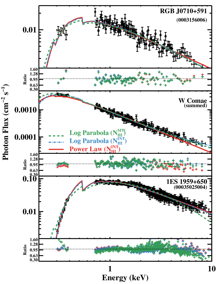
Figure 1: The best fit PL and LP models for the RGB J0710+591 Observation 0003156006, the W Comae summed exposure and the 1ES 1959+650 Observation 00035025004. The ratios of the data to models are shown in the bottom portion of each panel, with the dotted line drawn at a ratio of one. The PL model is shown with fitted N${}^{\rm INT}_{\rm HI}$ column density (red solid line), while the LP models are shown for both N${}^{\rm INT}_{\rm HI}$ lacking (green dashed line) and N${}^{\rm INT}_{\rm HI}$ contributing (blue dash-dotted line) column densities. The feature around $\sim$0.5 keV arises from the onset of the oxygen interaction cross-section. The fitted parameters are summarized in Tables 1, 3 and 4 in bold.

Table 1: Summary of spectral analysis RGB J0710+591 for absorbed PL and absorbed LP. When the possibility of N${}^{\rm INT}_{\rm HI}$ was included in the fits, the results were consistent with zero, providing similar fit parameters as found when N${}^{\rm INT}_{\rm HI}$ was set to zero. For the fits here, N${}^{\rm MW}_{\rm HI}$ was fixed to 4.16$\times 10^{20}$cm^-2 as measured by Kalberla et al. (2005) and N${}^{\rm INT}_{\rm HI}$ is set to zero. Observation ID 0003156006 is shown in bold and represents the best fit values for the models shown in the top panel of Figure 1.

Observation	Date	Mode	Exposure	Spectral		2-10 keV
ID				Data	PL	Flux	LP	LP	PL	LP
	[MJD]		[ks]	Counts	$\alpha$	[$\times 10^{-11}$ ergs cm-2s-1]	$\alpha$	$\beta$	$\chi^{2}$/dof	$\chi^{2}$/dof
0003156001	54882	pc	3.19	3348	1.76$\pm$0.03	3.5$\pm$0.1	1.68$\pm$0.06	0.1$\pm$0.1	81.82/82	80.14/81
0003156002	54887	pc	1.97	1491	1.83$\pm$0.05	3.3$\pm$0.2	1.6$\pm$0.1	0.3$\pm$0.2	31.13/37	29.3/36
0003156003	54888	pc	1.84	1978	1.81$\pm$0.04	3.6$\pm$0.1	1.71$\pm$0.08	0.2$\pm$0.1	62.55/48	61.01/47
0003156004	54889	wt	1.97	4231	1.77$\pm$0.03	5.1$\pm$0.2	1.78$\pm$0.05	-0.02$\pm$0.07	97.05/93	97/92
0003156005	54890	wt	1.91	2824	1.79$\pm$0.03	4.6$\pm$0.2	1.69$\pm$0.07	0.2$\pm$0.1	69.16/66	65.97/65
0003156006	54891	wt	2.19	4735	1.81$\pm$0.03	4.6$\pm$0.2	1.73$\pm$0.05	0.10$\pm$0.08	128.09/100	122.37/99
0003156007	54892	wt	1.97	4278	1.78$\pm$0.03	4.9$\pm$0.2	1.76$\pm$0.05	0.05$\pm$0.08	104.55/95	104.09/94
0003156008	55975	wt	1.25	1685	1.97$\pm$0.05	3.2$\pm$0.2	2.09$\pm$0.07	-0.3$\pm$0.1	37.64/39	33.42/38
0003156009	55978	wt	1.09	1375	2.07$\pm$0.06	1.9$\pm 0.2$	2.18$\pm$0.09	-0.2$\pm$0.2	21.16/31	19.53/30
0003156010	55985	wt	0.97	1286	1.93$\pm$0.06	2.5$\pm$0.2	2.2$\pm$0.1	-0.6$\pm$0.1	41.59/29	28.09/28
0003156011	55998	wt	1.15	1477	1.84$\pm$0.06	2.6$\pm$0.2	1.97$\pm$0.09	-0.3$\pm$0.1	31.44/34	28.68/33
0003156012	56002	wt	0.86	1154	1.91$\pm$0.06	2.6$\pm$0.2	2.1$\pm$0.1	-0.3$\pm$0.2	31.78/26	29.08/25
0003156013	56007	wt	1.03	1304	2.15$\pm$0.06	1.7$\pm$0.2	2.44$\pm$0.06	-0.8$\pm$0.1	72.35/28	43.7/27

Table 2: Summary of Swift XRT exposures of W Comae, summed for spectral analysis.

Observation	Date	Exposure	Source
ID	[MJD]	[ks]	Counts
0003092001	54223	2.45	194
0003092002	54225	4.56	503
0003092003	54226	3.70	403
00031160001	54539	4.38	458
00031160003	54541	2.15	173
00031160004	54553	1.68	436
00031160005	54554	1.63	168
00031219001	54624	8.98	4390
00031219002	54626	5.09	525
00035018001	53672	1.40	40
00031219002	53627	9.89	706
00031219003	53720	8.58	1050
00031219004	54495	2.26	94
00031219005	54499	4.56	122
00031219006	54528	2.06	327
00031219007	54536	1.86	80
00031219009	54589	1.72	264
00031219010	54828	1.52	74
00031219011	54835	1.03	110
00031219012	54842	0.98	60
00031219013	54844	0.94	92
00031219014	54856	0.66	209
00031219015	54863	1.12	189
00031219016	54870	1.31	167
00031219017	54877	0.96	112
00031219018	54884	1.35	372
00031219019	54891	1.54	138
00031219020	54898	1.19	64
00031219021	54912	1.59	96
00031219022	54919	0.87	39
00031219024	54933	0.98	48
00031219025	55175	4.81	182
00031219026	55230	1.02	60
00031219027	55237	1.04	21
00031219028	55245	1.18	45
00031219029	55251	1.23	14
00031219031	55265	0.88	25
00031219032	55272	0.94	174
00031219033	55279	1.09	34
00031219034	55286	0.73	270
00031219035	55293	0.93	549
00031219036	55300	1.16	893
00031219038	55314	1.35	367
00031219039	55335	0.95	297
00031219040	55356	1.97	668
00031219041	55599	0.97	267
00031219042	55605	0.89	370
00031219043	55612	1.12	475
00031219044	55626	1.09	579
00031219045	55636	0.96	235
00031219046	55641	1.19	290
00031219047	55648	1.14	353
00031219048	55661	0.95	374
00031219049	55669	1.20	1725
00031219050	55675	1.14	539
00031219051	55691	1.09	328
00031219053	55710	0.94	418
00031219054	55727	2.33	622
00031219055	55728	2.10	572
00031219056	55960	1.04	3143
00031219057	55967	1.16	358
00031219058	55974	1.33	414
00031219059	55981	1.03	289
00031219060	55988	1.47	454
00031219061	56002	0.92	338
00031219062	56010	1.37	661
00031219063	56023	1.01	334
00031219064	56037	0.88	294
00031219065	56042	0.92	289
00031219066	56053	0.99	283
00031219067	56058	1.05	449
00031219068	56065	1.02	766
00031219069	56072	1.05	364

Table 3: Summary of summed exposure spectral analysis for W Comae for an absorbed PL and LP model. The count rate for W Comae was low enough to require the summation of all photon counting mode exposures before grouping to 30 counts per bin. When N${}^{\rm INT}_{\rm HI}$ was included in the fits, the results were consistent with zero and provided redundant fit parameters as found when N${}^{\rm INT}_{\rm HI}$ was set to zero. For the fits quoted here, the N${}^{\rm MW}_{\rm HI}$ column density is fixed to 1.97$\times 10^{20}$cm^-2, as found in the LAB survey (Kalberla et al., 2005) and N${}^{\rm INT}_{\rm HI}$ is set to zero. The best fit models are shown for the summed exposure in the middle panel of Figure 1.

Exposure	Spectral	PL	2-10 keV Flux	LP	LP	PL	LP
[ks]	Counts	$\alpha$	[$\times 10^{-12}$ ergs cm-2s-1]	$\alpha$	$\beta$	$\chi^{2}$/dof	$\chi^{2}$/dof
132	9806	2.51$\pm$0.02	1.10$\pm$0.02	2.56$\pm$0.02	-0.13$\pm$0.04	191.94/174	163.52/173

Table 4: Summary of PL spectral analysis for 1ES 1959+650. Only windowed timing exposures of more than 500 seconds are included in this analysis. The Galactic N_HI column density was fixed to 1$\times 10^{21}$cm^-2, as measured by Kalberla et al. (2005) with a $\sim$3% error. Observation ID 00035025004 is shown in bold and represents the best fit values for the models shown in the bottom panel of Figure 1.

Observation	Date	Exposure	Fixed	PL	Free	2-10 keV Flux	Spectral	Fixed	Free
ID			PL	N${}^{\rm MW}_{\rm HI}$+N${}^{\rm INT}_{\rm HI}$	PL	$\times 10^{-11}$	Counts	PL	PL
	[MJD]	[ks]	$\alpha$	[$\times 10^{21}$cm-2]	$\alpha$	[ergs cm-2s-1]		$\chi^{2}$/dof	$\chi^{2}$/dof
00035025001	53479	4.43	2.102$\pm$0.008	1.852$\pm$0.004	2.40$\pm$0.02	13.7$\pm$0.1	32782	1019.0/330	380.3/329
00035025002	53874	1.43	2.01$\pm$0.02	1.943$\pm$0.009	2.32$\pm$0.03	13.3$\pm$0.3	9270	426.3/192	223.1/191
00035025003	53876	1.99	1.97$\pm$0.01	1.846$\pm$0.007	2.22$\pm$0.02	18.1$\pm$0.3	14911	510.3/251	289.5/250
00035025004	53878	5.35	1.91$\pm$0.01	1.753$\pm$0.004	2.13$\pm$0.01	25.3$\pm$0.2	44642	1019.0/417	500.8/416
00035025005	53879	2.30	1.90$\pm$0.01	1.960$\pm$0.006	2.19$\pm$0.02	28.2$\pm$0.4	26758	804.9/328	384.1/327
00035025006	53880	4.38	1.95$\pm$0.008	1.957$\pm$0.005	2.22$\pm$0.01	23.1$\pm$0.3	44306	1211.8/401	483.8/400
00035025007	53881	4.37	1.975$\pm$0.008	1.865$\pm$0.004	2.23$\pm$0.01	22.3$\pm$0.3	43562	1119.9/396	480.4/397
00035025008	53882	4.28	2.078$\pm$0.008	2.147$\pm$0.005	2.43$\pm$0.02	17.0$\pm$0.2	36841	1430.8/343	458.0/342
00035025009	53883	4.41	2.067$\pm$0.008	2.117$\pm$0.005	2.41$\pm$0.02	17.3$\pm$0.2	35858	1265.9/344	429.3/343
00035025010	53884	3.28	2.12$\pm$0.01	2.001$\pm$0.006	2.44$\pm$0.02	15.4$\pm$0.2	26439	914.7/244	383.6/243
00035025016	54434	1.28	2.07$\pm$0.06	3.192$\pm$0.058	2.5$\pm$0.1	17.8$\pm$1.6	1268	56.0/37	40.2/36
00035025027	54989	0.99	2.26$\pm$0.02	1.899$\pm$0.011	2.56$\pm$0.04	10.5$\pm$0.3	6399	267.0/150	165.9/149
00035025028	54996	1.0	2.33$\pm$0.03	1.542$\pm$0.011	2.52$\pm$0.05	8.18$\pm$0.4	4749	147.1/120	116.3/119
00035025032	55010	1.55	2.17$\pm$0.02	1.587$\pm$0.008	2.36$\pm$0.03	12.8$\pm$0.2	9745	239.2/195	166.1/194
00035025034	55016	1.64	2.11$\pm$0.02	1.693$\pm$0.008	2.32$\pm$0.03	16.8$\pm$6.1	12162	329.9/219	210.1/218
00035025037	55038	0.60	2.28$\pm$0.03	1.762$\pm$0.015	2.56$\pm$0.06	8.91$\pm$0.3	3331	126.2/84	87.6/83
00035025038	55045	0.65	2.19$\pm$0.03	1.927$\pm$0.014	2.46$\pm$0.05	12.3$\pm$0.5	4687	179.2/120	116.6/119
00035025041	55066	1.20	2.17$\pm$0.02	1.439$\pm$0.011	2.31$\pm$0.04	9.88$\pm$0.4	5488	144.4/139	124.3/138
00035025042	55070	1.23	2.15$\pm$0.02	1.989$\pm$0.011	2.48$\pm$0.04	11.6$\pm$0.4	7914	330.5/175	177.0/174
00035025043	55087	0.96	2.27$\pm$0.03	1.575$\pm$0.011	2.47$\pm$0.05	78.1$\pm$0.3	4693	140.4/120	106.1/119
00035025044	55100	6.12	2.256$\pm$0.009	1.646$\pm$0.004	2.47$\pm$0.02	80.6$\pm$0.1	30252	619.9/303	320.2/302
00035025045	55318	1.29	2.07$\pm$0.02	1.606$\pm$0.012	2.24$\pm$0.04	80.6$\pm$0.1	4836	180.6/122	151.3/121
00035025046	55323	1.09	2.03$\pm$0.02	1.584$\pm$0.012	2.18$\pm$0.04	13.2$\pm$2.4	6433	163.0/159	129.2/158
00035025047	55332	1.02	2.07$\pm$0.02	1.333$\pm$0.011	2.17$\pm$0.04	11.2$\pm$0.3	5188	124.0/132	113.9/131
00035025048	55346	1.12	2.07$\pm$0.03	1.622$\pm$0.014	2.24$\pm$0.04	9.94$\pm$0.4	5081	122.1/130	94.3/129
00035025049	55353	1.08	2.05$\pm$0.03	2.152$\pm$0.020	2.32$\pm$0.05	7.83$\pm$0.3	4252	154.0/107	95.8/106
00035025050	55360	1.07	2.13$\pm$0.03	2.548$\pm$0.023	2.52$\pm$0.06	7.37$\pm$0.3	4026	206.2/100	98.5/99
00035025051	55367	1.01	2.16$\pm$0.03	1.967$\pm$0.020	2.43$\pm$0.06	5.68$\pm$0.2	3326	103.1/82	62.8/81
00035025052	55375	1.16	2.16$\pm$0.03	1.536$\pm$0.014	2.32$\pm$0.05	7.77$\pm$0.3	4708	182.2/121	161.2/120
00035025053	55381	1.16	2.03$\pm$0.02	2.046$\pm$0.017	2.29$\pm$0.05	9.76$\pm$0.3	5703	227.1/145	165.2/144
00035025054	55396	1.11	2.14$\pm$0.03	2.019$\pm$0.016	2.41$\pm$0.05	7.64$\pm$0.3	4644	167.6/118	104.7/117
00035025056	55404	0.77	2.23$\pm$0.03	1.710$\pm$0.017	2.44$\pm$0.06	8.48$\pm$0.4	3273	129.5/83	104.9/82
00035025057	55409	1.02	2.34$\pm$0.03	1.961$\pm$0.016	2.68$\pm$0.06	4.94$\pm$0.2	3628	137.1/93	73.6/92
00035025058	55458	1.26	2.17$\pm$0.02	1.921$\pm$0.012	2.46$\pm$0.04	8.69$\pm$0.4	6132	242.4/147	143.1/146
00035025059	55463	1.24	2.01$\pm$0.02	1.798$\pm$0.010	2.24$\pm$0.03	15.7$\pm$0.4	9237	313.8/193	205.7/192
00035025062	55686	1.19	2.50$\pm$0.03	1.483$\pm$0.012	2.69$\pm$0.05	3.36$\pm$0.2	3247	115.0/81	92.8/80
00035025063	55693	1.25	2.48$\pm$0.04	1.630$\pm$0.018	2.70$\pm$0.07	2.43$\pm$0.1	2438	91.4/66	72.9/65
00035025064	55700	0.94	2.31$\pm$0.03	1.689$\pm$0.018	2.50$\pm$0.06	5.59$\pm$0.2	3361	109.9/83	90.6/82
00035025066	55714	0.95	2.09$\pm$0.03	2.111$\pm$0.022	2.35$\pm$0.06	7.68$\pm$0.3	3804	127.1/94	88.2/93
00035025067	55721	0.98	2.22$\pm$0.03	2.060$\pm$0.018	2.53$\pm$0.06	7.58$\pm$0.3	3625	151.6/93	94.7/92
00035025068	55728	1.0	2.28$\pm$0.04	1.632$\pm$0.027	2.46$\pm$0.09	3.35$\pm$0.2	2001	63.2/53	54.9/52
00035025069	55735	1.17	2.29$\pm$0.04	1.968$\pm$0.032	2.54$\pm$0.09	2.74$\pm$0.2	2073	71.3/56	54.6/55
00035025071	55749	1.00	2.36$\pm$0.06	1.255$\pm$0.026	2.4$\pm$0.1	2.12$\pm$0.2	1442	39.5/40	38.5/39
00035025072	55763	1.05	2.32$\pm$0.04	2.696$\pm$0.034	2.77$\pm$0.09	3.01$\pm$0.2	2364	127.8/63	74.1/62
00035025074	55814	1.41	2.10$\pm$0.02	2.276$\pm$0.012	2.42$\pm$0.03	33.9$\pm$0.9	11257	442.4/216	233.1/215
00035025075	56036	0.98	2.44$\pm$0.03	1.652$\pm$0.012	2.67$\pm$0.05	9.97$\pm$0.3	5504	156.7/130	112.4/129
00035025076	56037	1.52	2.36$\pm$0.02	1.678$\pm$0.007	2.60$\pm$0.03	10.8$\pm$0.2	11140	337.4/195	220.7/194
00035025077	56051	0.99	2.34$\pm$0.02	1.592$\pm$0.012	2.52$\pm$0.04	9.23$\pm$0.2	6044	154.6/142	117.5/141
00035025078	56064	1.06	2.24$\pm$0.02	1.525$\pm$0.011	2.41$\pm$0.04	10.8$\pm$0.3	5500	161.6/135	130.2/134
00035025079	56067	0.69	2.23$\pm$0.03	1.574$\pm$0.018	2.38$\pm$0.06	9.79$\pm$0.3	3841	116.6/94	103.4/93
00035025080	56074	1.27	2.10$\pm$0.02	2.150$\pm$0.013	2.40$\pm$0.05	13.1$\pm$0.3	9006	370.5/187	232.1/186
00035025081	56075	1.10	2.28$\pm$0.02	1.631$\pm$0.012	2.48$\pm$0.04	7.59$\pm$0.3	5230	145.3/127	108.2/126
00035025082	56076	0.92	2.40$\pm$0.03	1.643$\pm$0.018	2.60$\pm$0.06	4.77$\pm$0.3	3207	105.4/82	85.2/81
00035025083	56078	1.04	2.15$\pm$0.02	1.966$\pm$0.014	2.42$\pm$0.04	10.9$\pm$0.4	6148	214.9/147	138.3/146
00035025084	56079	1.52	2.37$\pm$0.02	1.759$\pm$0.014	2.44$\pm$0.04	9.75$\pm$0.3	7082	210.1/161	167.7/160
00035025085	56094	0.99	2.40$\pm$0.03	1.488$\pm$0.012	2.57$\pm$0.05	7.32$\pm$0.3	4448	155.1/113	135.8/112
00035025086	56107	1.01	2.09$\pm$0.02	1.722$\pm$0.012	2.28$\pm$0.04	16.7$\pm$0.5	6083	212.7/155	159.3/154
00035025087	56128	1.01	2.16$\pm$0.03	1.590$\pm$0.016	2.32$\pm$0.05	13.2$\pm$0.5	3916	84.0/97	66.3/96
00035025088	56135	1.18	2.27$\pm$0.03	1.927$\pm$0.017	2.54$\pm$0.05	8.65$\pm$0.3	4892	153.7/126	103.1/125
00035025089	56179	0.93	2.48$\pm$0.03	1.167$\pm$0.011	2.53$\pm$0.05	4.74$\pm$0.3	3142	98.2/77	96.1/76
00035025091	56196	1.52	2.38$\pm$0.03	1.721$\pm$0.017	2.59$\pm$0.06	4.01$\pm$0.2	3934	119.7/99	91.8/98

Table 5: Summary of LP spectral analysis for 1ES 1959+650. Observation ID details given in Table 3. The Galactic N_HI column density was fixed to 1$\times 10^{21}$cm^-2, as measured by Kalberla et al. (2005) with a $\sim$3% error. Observation ID 00035025004 is shown in bold and represents the best fit values for the models shown in the bottom panel of Figure 1.

Observation	Fixed	Fixed	Free	Free	Free	Spectral	Fixed	Free
ID	LP	LP	LP NHI	LP	LP	Counts	LP	LP
	$\alpha$	$\beta$	[$\times 10^{22}$cm-2]	$\alpha$	$\beta$		$\chi^{2}$/dof	$\chi^{2}$/dof
00035025001	1.83$\pm$0.02	0.68$\pm$0.03	0.15$\pm$0.01	2.16$\pm$0.07	0.29$\pm$0.086	32782	390.1/329	363.8/328
00035025002	1.73$\pm$0.03	0.69$\pm$0.06	0.18$\pm$0.03	2.2$\pm$0.1	0.1$\pm$0.2	9270	239.7/191	222.1/190
00035025003	1.69$\pm$0.03	0.62$\pm$0.05	0.14$\pm$0.02	1.9$\pm$0.1	0.4$\pm$0.1	14911	274.6/250	264.1/249
00035025004	1.51$\pm$0.03	0.42$\pm$0.03	0.17$\pm$0.01	2.09$\pm$0.06	0.06$\pm$0.07	44642	537.6/416	481.1/415
00035025005	1.59$\pm$0.02	0.63$\pm$0.04	0.17$\pm$0.01	1.98$\pm$0.08	0.21$\pm$0.09	26758	403.5/327	378.9/326
00035025006	1.67$\pm$0.02	0.62$\pm$0.03	0.19$\pm$0.01	2.16$\pm$0.06	0.07$\pm$0.07	44306	553.6/400	482.8/399
00035025007	1.72$\pm$0.03	0.57$\pm$0.03	0.18$\pm$0.01	2.19$\pm$0.06	0.04$\pm$0.07	43562	549.0/395	480.1/394
00035025008	1.74$\pm$0.02	0.79$\pm$0.03	0.19$\pm$0.01	2.29$\pm$0.07	0.17$\pm$0.08	36841	519.9/342	453.9/341
00035025009	1.75$\pm$0.02	0.75$\pm$0.03	0.20$\pm$0.01	2.36$\pm$0.07	0.06$\pm$0.08	35858	503.1/343	428.8/342
00035025010	1.83$\pm$0.02	0.71$\pm$0.04	0.19$\pm$0.01	2.36$\pm$0.08	0.1$\pm$0.1	26439	422.8/243	382.7/242
00035025016	1.5$\pm$0.2	1.2$\pm$0.3	0.1$\pm$0.2	1.48$\pm$0.9	1.15$\pm$1.0	1268	38.8/36	38.8/35
00035025027	2.00$\pm$0.04	0.67$\pm$0.08	0.16$\pm$0.03	2.4$\pm$0.2	0.2$\pm$0.2	6399	169.2/149	164.7/148
00035025028	2.18$\pm$0.04	0.39$\pm$0.08	0.17$\pm$0.03	2.6$\pm$0.2	-0.1$\pm$0.2	4749	121.6/119	116.0/118
00035025032	1.99$\pm$0.03	0.42$\pm$0.06	0.15$\pm$0.02	2.3$\pm$0.1	0.1$\pm$0.2	9745	172.0/194	165.9/193
00035025034	1.89$\pm$0.03	0.48$\pm$0.05	0.15$\pm$0.02	2.2$\pm$0.1	0.1$\pm$0.1	12162	217.0/218	208.9/217
00035025037	2.09$\pm$0.05	0.57$\pm$0.1	0.20$\pm$0.04	2.7$\pm$0.3	-0.2$\pm$0.3	3331	92.6/83	87.3/82
00035025038	1.91$\pm$0.05	0.63$\pm$0.09	0.15$\pm$0.04	2.2$\pm$0.2	0.3$\pm$0.2	4687	117.2/119	115.1/118
00035025041	2.05$\pm$0.04	0.27$\pm$0.08	0.17$\pm$0.03	2.5$\pm$0.2	-0.2$\pm$0.2	5488	129.6/138	123.3/137
00035025042	1.88$\pm$0.04	0.67$\pm$0.07	0.20$\pm$0.03	2.5$\pm$0.2	-0.01$\pm$0.2	7914	194.2/174	177.0/173
00035025043	2.10$\pm$0.04	0.45$\pm$0.09	0.13$\pm$0.03	2.3$\pm$0.2	0.2$\pm$0.2	4693	106.2/119	105.2/118
00035025044	2.05$\pm$0.02	0.51$\pm$0.03	0.11$\pm$0.01	2.12$\pm$0.07	0.43$\pm$0.08	30252	296.1/302	295.1/301
00035025045	1.85$\pm$0.05	0.47$\pm$0.08	0.07$\pm$0.03	1.7$\pm$0.2	0.64$\pm$0.2	4836	143.3/121	142.5/120
00035025046	1.84$\pm$0.04	0.38$\pm$0.07	0.14$\pm$0.03	2.1$\pm$0.2	0.1$\pm$0.2	6433	130.7/158	128.6/157
00035025047	1.91$\pm$0.05	0.323$\pm$0.08	0.05$\pm$0.02	1.6$\pm$0.2	0.7$\pm$0.2	5188	105.8/131	101.6/130
00035025048	1.87$\pm$0.05	0.42$\pm$0.09	0.14$\pm$0.03	2.1$\pm$0.2	0.2$\pm$0.2	5081	95.0/129	93.7/128
00035025049	1.68$\pm$0.06	0.69$\pm$0.1	0.13$\pm$0.04	1.9$\pm$0.2	0.5$\pm$0.2	4252	92.5/106	91.7/105
00035025050	1.67$\pm$0.07	0.93$\pm$0.1	0.19$\pm$0.05	2.2$\pm$0.3	0.4$\pm$0.3	4026	101.5/99	96.3/98
00035025051	1.88$\pm$0.07	0.63$\pm$0.1	0.17$\pm$0.05	2.3$\pm$0.3	0.2$\pm$0.3	3326	65.3/81	62.5/80
00035025052	2.00$\pm$0.05	0.34$\pm$0.09	0.16$\pm$0.03	2.4$\pm$0.2	0.0$\pm$0.2	4708	165.1/120	161.1/119
00035025053	1.68$\pm$0.06	0.68$\pm$0.09	0.11$\pm$0.03	1.8$\pm$0.2	0.6$\pm$0.2	5703	158.3/143	158.1/142
00035025054	1.81$\pm$0.06	0.7$\pm$0.1	0.13$\pm$0.04	2.0$\pm$0.2	0.5$\pm$0.2	4644	101.0/117	100.2/116
00035025056	2.00$\pm$0.06	0.5$\pm$0.1	0.14$\pm$0.04	2.2$\pm$0.3	0.2$\pm$0.3	3273	105.4/82	104.5/81
00035025057	2.09$\pm$0.06	0.7$\pm$0.1	0.18$\pm$0.04	2.6$\pm$0.3	0.1$\pm$0.3	3628	78.1/92	73.6/91
00035025058	1.90$\pm$0.04	0.66$\pm$0.08	0.16$\pm$0.03	2.3$\pm$0.2	0.2$\pm$0.2	6132	146.8/146	141.7/145
00035025059	1.76$\pm$0.04	0.55$\pm$0.06	0.15$\pm$0.02	2.1$\pm$0.1	0.2$\pm$0.2	9237	210.1/192	204.2/191
00035025062	2.34$\pm$0.05	0.5$\pm$0.1	0.07$\pm$0.03	2.1$\pm$0.2	0.7$\pm$0.3	3247	87.5/80	86.7/79
00035025063	2.30$\pm$0.07	0.5$\pm$0.1	0.16$\pm$0.05	2.7$\pm$0.3	0.1$\pm$0.4	2438	74.4/65	72.8/64
00035025064	2.06$\pm$0.07	0.5$\pm$0.1	0.07$\pm$0.03	1.9$\pm$0.2	0.7$\pm$0.3	3361	84.7/82	84.1/81
00035025066	1.75$\pm$0.07	0.7$\pm$0.1	0.14$\pm$0.05	2.0$\pm$0.2	0.4$\pm$0.3	3804	86.8/93	86.0/92
00035025067	1.88$\pm$0.06	0.8$\pm$0.1	0.10$\pm$0.04	1.9$\pm$0.2	0.8$\pm$0.3	3625	88.3/92	88.3/91
00035025068	2.09$\pm$0.09	0.4$\pm$0.2	0.16$\pm$0.07	2.4$\pm$0.4	0$\pm$0.5	2001	55.8/52	54.9/51
00035025069	2.0$\pm$0.1	0.6$\pm$0.2	0.23$\pm$0.09	2.7$\pm$0.4	-0.2$\pm$0.5	2073	58.0/55	54.4/54
00035025071	2.3$\pm$0.1	0.2$\pm$0.2	0.12$\pm$0.07	2.4$\pm$0.4	0.1$\pm$0.6	1442	38.5/39	38.5/38
00035025072	1.9$\pm$0.1	1.0$\pm$0.2	0.24$\pm$0.09	2.6$\pm$0.4	0.2$\pm$0.5	2364	78.2/62	74.0/61
00035025074	1.68$\pm$0.04	0.83$\pm$0.07	0.11$\pm$0.02	1.8$\pm$0.1	0.7$\pm$0.1	11257	209.2/215	208.9/214
00035025075	2.25$\pm$0.04	0.53$\pm$0.09	0.13$\pm$0.03	2.4$\pm$0.2	0.3$\pm$0.3	5504	111.8/129	110.9/128
00035025076	2.16$\pm$0.03	0.54$\pm$0.05	0.11$\pm$0.02	2.2$\pm$0.1	0.5$\pm$0.1	11140	211.7/194	211.4/193
00035025077	2.16$\pm$0.04	0.41$\pm$0.08	0.15$\pm$0.03	2.4$\pm$0.2	0.1$\pm$0.2	6044	120.4/141	117.3/140
00035025078	2.1$\pm$0.2	0.4$\pm$0.2	0.11$\pm$0.03	2.1$\pm$0.2	0.4$\pm$0.2	5500	127.1/134	127.1/133
00035025079	2.02$\pm$0.07	0.4$\pm$0.1	0.09$\pm$0.04	1.9$\pm$0.2	0.5$\pm$0.3	3841	100.2/93	100.1/92
00035025080	1.75$\pm$0.04	0.76$\pm$0.07	0.13$\pm$0.03	1.9$\pm$0.2	0.6$\pm$0.2	9006	223.6/186	222.4/185
00035025081	2.07$\pm$0.05	0.51$\pm$0.08	0.08$\pm$0.03	1.9$\pm$0.2	0.7$\pm$0.2	5230	100.1/126	97.6/125
00035025082	2.20$\pm$0.07	0.5$\pm$0.1	0.13$\pm$0.04	2.4$\pm$0.3	0.2$\pm$0.3	3207	85.4/80	84.6/79
00035025083	1.85$\pm$0.05	0.65$\pm$0.09	0.15$\pm$0.03	2.1$\pm$0.2	0.3$\pm$0.2	6148	138.5/146	135.9/145
00035025084	1.98$\pm$0.05	0.53$\pm$0.08	0.10$\pm$0.03	2.0$\pm$0.2	0.5$\pm$0.2	7082	161.6/160	161.6/159
00035025085	2.24$\pm$0.05	0.4$\pm$0.1	0.10$\pm$0.03	2.2$\pm$0.2	0.4$\pm$0.3	4448	133.4/112	133.4/111
00035025086	1.81$\pm$0.04	0.55$\pm$0.08	0.08$\pm$0.02	1.7$\pm$0.2	0.7$\pm$0.2	6083	146.2/154	145.6/153
00035025087	1.96$\pm$0.06	0.4$\pm$0.1	0.11$\pm$0.03	2.1$\pm$0.2	0.3$\pm$0.2	3916	65.3/96	65.0/95
00035025088	2.00$\pm$0.06	0.6$\pm$0.1	0.16$\pm$0.04	2.4$\pm$0.2	0.2$\pm$0.3	4892	105.2/125	102.4/124
00035025089	2.39$\pm$0.05	0.2$\pm$0.1	0.03$\pm$0.03	1.9$\pm$0.2	0.8$\pm$0.3	3142	92.9/76	88.4/75
00035025091	2.13$\pm$0.06	0.6$\pm$0.1	0.10$\pm$0.04	2.2$\pm$0.2	0.5$\pm$0.3	3934	89.5/98	89.5/97

References

- Abdo et al. (2010a) Abdo, A. A., Ackermann, M., Agudo, I. et al. 2010, ApJ, 716, 30
- Abramowski et al. (2012) Abramowski, A., Acero, F., Aharonian, F. et al. 2012, A&A, 539, 149
- Abrassart & Czerny (2000) Abrassart, A. & Czerny, B. 2000, A&A, 356, 475
- Acciari et al. (2009) Acciari, V. A., Aliu, E., Aune, T. et al. 2009, ApJ, 707, 612
- Acciari, et al. (2010) Acciari, V. A.. Aliu, E., Arlen, T. et al. 2010, ApJ, 715, 49
- Achterberg et al. (2001) Achterberg, A., Gallant, Y., Kirk, J. & Guthmann, A. 2001, MNRAS, 328, 393
- Aharonian et al. (2002) Aharonian, F. A. et al. Phys. Rev. D., 66, 1
- Aleksić et al. (2012) Aleksić J., Alvarez, E. A., Antonelli, L. A. et al. 2012, A&A, 525, 100
- Aliu et al. (2011) Aliu, E., Aune, T., Beilicke, M., et al. 2011, ApJ, 742, 127
- Arnal et al. (2000) Arnal et al. 2000, A&AS, 142, 35
- Aliu et al. (2012) Aliu, E., Aune, T., Beilick, M., et al. 2012, ApJ, submitted
- Bajaja et al. (2005) Bajaja et al. 2005, A&A, 440, 767
- Bednarek (1993) Bednarek, W. 1993, ApJL, 402, 29
- Böttcher & Chiang (2002) Böttcher, M., & Chiang, J. 2002, ApJ, 581, 127
- Böttcher (2005) Böttcher, M., 2005, ApJ, 621, 175 (Erratum: ApJ, 641, 1233 [2006])
- Burrows et al. (2005) Burrows et al., 2005, Space Sci. Rev., 120, 165
- Costamante (2001) Costamante, L. et al. 2001, A&A, 371, 512
- Dermer et al. (1992) Dermer, C., Schlickeiser, R., Mastichiadis, A. 1992, A&A, 256, 27
- Dermer et al. (2012) Dermer, C., Murase, K., & Takami, H. 2012, ApJ, 755, 147
- Evans et al. (2009) Evans, P., Beardmore, A. P. Page, K. L. et al. 2009, MNRAS, 397, 1177
- Fossati et al. (1998) Fossati, G., Maraschi, L., Celotti, A., Comastri, A., Ghisellini, G. 1998, MNRAS, 299, 433
- Fumagalli et al. (2012) Fumagalli, M., Dessauges-Zavadsky, M., Furniss, A. et al. 2012, MNRAS, 424, 227
- Gehrels et al. (2004) Gehrels, N., Chincarini, G., Giommi, P et al. 2004, ApJ, 611, 1005
- Ghisellini & Tavecchio (2008) Ghisellini, G. & Tavecchio, F. 2008, MNRAS, 387, 1669
- Glover & Clark (2012) Glover, S. & Clark, P. C. 2012, MNRAS, 421, 9
- Hartmann & Burton (1997) Hartmann, D., & Burton, W. B. 1997, Atlas of Galactic Neutral Hydrogen (Cambridge University Press), ISBN 0521471117
- Kalberla et al. (2005) Kalberla, P., Burton, W., Hartmann, D. et al. 2005, A&A, 440, 775
- Krawczynski et al. (2004) Krawczynski, H. et al. 2004, ApJ, 601, 151
- Krumholz et al. (2009) Krumholz, M. McKee, C. F., &Tumlinson, J. 2009, ApJ 693, 216
- Maraschi et al. (1992) Maraschi, L., Ghisellini, G. Celotti, A. 1992, ApJL, 397, 5
- Massaro et al. (2004) Massaro, F. et al. 2004, A&A, 413, 489
- Massaro et al. (2006) Massaro, F. et al. 2006, A&A, 448, 861
- Massaro et al. (2008) Massaro, F., Tramacere, A., Cavaliere, A., Perri, M. & Giommi, P. 2008, A&A, 478, 395
- Meyer et al. (2011) Meyer, E. et al 2011, ApJ, 740, 98
- Morrison & McCammon (1983) Morrison, R. & McCammon, D. 1983, ApJ, 270, 119
- Mücke et al. (2003) Mücke, A., Protheroe, R., Engel, R., Rachen, J. P. & Stanev, T. 2003, APh, 18, 593
- Mushotzky et al. (1993) Mushotzky, R., Done, C. & Pounds, K. 1993, ARA&A, 31, 717
- Paggi et al. (2009) Paggi, A., Massaro, F., Vittorini, V. et al. 2009, A&A, 504, 821
- Perlman et al. (2005) Perlman, E. Madejski, G., Georganopoulos, M. et al. 2005, ApJ, 625, 727
- Rybicki & Lightman (1979) Rybicki, G. B. & Lightman, A. P. 1979, Radiative Processes in Astrophysics (New York:Wiley)
- Summerlin & Baring (2012) Summerlin, E. & Baring, M. 2012, ApJ, 745, 63
- Tagliaferri et al. (2003) Tagliaferri, G. et al. 2003, A&A, 412, 711
- Tavecchio et al. (2002) Tavecchio, F., Maraschi, L., Ghisellini, G. et al. 2002, ApJ, 575, 137
- Tielenn & Hollenbach (1985) Tielenn & Hollenbach, D. 1985, ApJ, 291, 722
- Tramacere et al. (2011) Tramacere, A., Massaro, E. & Taylor, A. M. 2011, ApJ, 739, 66
- Tramacere et al. (2007) Tramacere, A. et al. 2007, A&A, 467, 501
- Wachter et al. (1988) Wachter, K., Strauss, M. & Filippenko, A. 1988, ApJ, 330, 91
- Vagnetti et al. (2011) Vagnetti, F., Turriziani, S. & Trevese, D. 2011, A&A, 536, 84
- Virtanen & Vainio (2005) Virtanen, J. & Vainio, R. 2005, ApJ, 621, 313