Imaginary-time nonuniform mesh method for solving the multidimensional Schrödinger equation: Fermionization and melting of quantum Lennard-Jones crystals

Abstract

An imaginary-time nonuniform mesh method is presented and used to find the first 50 eigenstates and energies of up to five strongly interacting spinless quantum Lennard-Jones particles trapped in a one-dimensional harmonic potential. We show that the use of tailored grids reduces drastically the computational effort needed to diagonalize the Hamiltonian and results in a favorable scaling with dimensionality. Solutions to both bosonic and fermionic counterparts of this strongly interacting system are obtained, the bosonic case clustering as a Tonks-Girardeau crystal exhibiting the phenomenon of fermionization. The numerically exact excited states are used to describe the melting of this crystal at finite temperature.

The multidimensional Schrödinger equation (MDSE) is undoubtedly one of the cornerstones of modern physics and much attention has been paid to developing efficient numerical methods for finding its solutions Harris et al. (1965); Kosloff (1988); Shimshovitz and Tannor (2012); Pollet (2012); Parr and Yang (1994); Dalfovo et al. (1995); Savenko et al. (2013); Rogel-Salazar (2013); Billing and Adhikari (2000); Runge and Gross (1984); Abid et al. (2003); Wyatt and Trahan (2005); Alvarez et al. (2011); Tkatchenko et al. (2012); Martín-Delgado and Sierra (1996); Corney and Drummond (2004); Torres-Vega and Frederick (1991); McMahon et al. (2012). A very rich testing ground for such methods has been provided by the observation of new quantum phases at ultracold temperatures in finite and homogeneous systems McMahon et al. (2012); Kapitza (1938); Leggett (1972); Grebenev et al. (2000); Anglin and Ketterle (2002); Balibar (2010), and also by the development of optical lattices where ultracold atoms are trapped Bloch (2005). Due to their fascinating structural and dynamical properties, special attention has been recently devoted to one-dimensional traps Ronzheimer et al. (2013); Panfil et al. (2013); Vignolo and Minguzzi (2013); Gring et al. (2012); Kinoshita et al. (2006); Paredes et al. (2004). Indeed, in the strongly interacting (Tonks-Girardeau) regime of bosonic particles trapped in one-dimensional geometries, the repulsive nature of the atomic interaction at short distances gives rise to the phenomenon known as fermionization, the mechanism of which is actively studied both theoretically and experimentally.

Rigorous description and explanation of the new physics found in these well-controlled experiments require accurate theoretical methods and constitute a formidable challenge Bloch et al. (2008), the main technical difficulty being the scaling of numerical algorithms with the number of dimensions $D$. Indeed, standard algorithms for solving differential equations, such as the Finite Difference method, scale exponentially with dimensions Morton and Mayers (2005), making numerical solutions of many-dimensional problems impracticable, if not impossible. Improved methods addressing this difficulty in the case of stationary states include the Discrete Variable Representation (DVR) Harris et al. (1965), collocation method Kosloff (1988), phase-space method based on von Neumann periodic lattice Shimshovitz and Tannor (2012), variational or diffusion quantum Monte Carlo (MC) methods McMahon et al. (2012); Pollet (2012), Density Functional Theory (DFT) McMahon et al. (2012); Parr and Yang (1994), mean-field or pseudopotential interaction models Dalfovo et al. (1995); Savenko et al. (2013); Rogel-Salazar (2013), and many others. Some of these methods find only the ground state of the time-independent MDSE, using different efficient techniques such as the imaginary time (IT) propagation Popov (2005) or the Variational Principle Sakurai (1993). Methods for real-time quantum dynamics include the Time-Dependent DVR Billing and Adhikari (2000), DFT Runge and Gross (1984), mean-field approaches Abid et al. (2003), trajectory-based methods such as Bohmian dynamics Wyatt and Trahan (2005), or time-dependent density matrix renormalization group (t-DMRG) method Alvarez et al. (2011), which has proven to be very efficient in one-dimensional geometries. Despite many accomplishments in special cases, finding excited states and describing the real-time dynamics governed by a general high-dimensional Hamiltonian in the strongly interacting regime remains a difficult computational challenge.

In this paper we propose a novel general method, scaling favorably with dimensions, which is able to solve the time-independent MDSE numerically exactly and simultaneously finds both its ground and excited states. Obviously, the proposed IT nonuniform mesh method (ITNUMM) is not intended to replace other well established approaches; instead we expect it to have a domain of applicability where other methods present more technical difficulties, such as in finding excited states of many-dimensional systems and where efficiency is more important than high accuracy. To show that ITNUMM achieves these goals, we apply it to find the wavefunctions of the first 50 states of an ensemble of up to five distinguishable Lennard-Jones (LJ) spinless particles trapped in a one-dimensional harmonic potential in the Tonks-Girardeau regime. Once these states are obtained, we find, via symmetrization and anti-symmetrization, the solutions for the Bose-Einstein and Fermi-Dirac statistics, respectively, and observe fermionization in the bosonic case. We also show that the computed excited states can be used in a thermal average to describe the melting of the LJ clusters at finite temperature. As we use no other approximation than the numerical discretization of space and time, the obtained results are numerically exact.

The derivation of our method starts by rewriting the time-dependent MDSE Sakurai (1993)

$$i\hbar\frac{d}{dt}|\psi(t)\rangle=\mathcal{H}|\psi(t)\rangle,$$ (1)

where $|\psi(t)\rangle$ is the quantum state at time $t$ of the $D$-dimensional system described by Hamiltonian $\mathcal{H}$, in terms of the quantum propagator $K({\mathbf{q}},{\mathbf{q}}^{\prime};t-t^{\prime}):=\langle{\mathbf{q}}|e^{-i(t-t^{\prime})\mathcal{H}/\hbar}|{\mathbf{q}}^{\prime}\rangle$ in the position basis $|{\mathbf{q}}\rangle$:

$$\psi({\mathbf{q}},t)=\int d{\mathbf{q}}^{\prime}K({\mathbf{q}},{\mathbf{q}}^{\prime};t-t^{\prime})\psi({\mathbf{q}}^{\prime},t^{\prime}).$$ (2)

Hamiltonian $\mathcal{H}:=\mathcal{H}_{0}+\mathcal{H}_{1}$ is now split into two components: $\mathcal{H}_{0}$ is any Hamiltonian that includes the kinetic energy operator $\mathcal{T}$ and whose matrix elements in the ${\mathbf{q}}$-representation are known, while $\mathcal{H}_{1}\equiv\mathcal{H}_{1}({\mathbf{q}})$ is any many-body potential depending only on ${\mathbf{q}}$. For very short time intervals $t-t^{\prime}=\Delta t$, the time evolution operator can be split to first order as $e^{-i\Delta t\mathcal{H}/\hbar}=e^{-i\Delta t\mathcal{H}_{0}/\hbar}e^{-i\Delta t\mathcal{H}_{1}/\hbar}+O(\Delta t^{2})$ and one can write

$$\psi({\mathbf{q}},t^{\prime}+\Delta t) =\int d{\mathbf{q}}^{\prime}K_{0}({\mathbf{q}},{\mathbf{q}}^{\prime};\Delta t)e^{-i\Delta t\mathcal{H}_{1}({\mathbf{q}}^{\prime})/\hbar}\psi({\mathbf{q}}^{\prime},t^{\prime})$$

$$\ +O(\Delta t^{2}),$$ (3)

where $K_{0}({\mathbf{q}},{\mathbf{q}}^{\prime};\Delta t):=\langle{\mathbf{q}}|e^{-i\Delta t\mathcal{H}_{0}/\hbar}|{\mathbf{q}}^{\prime}\rangle$ is the propagator of $\mathcal{H}_{0}$, which is assumed to be known explicitly.

The $|{\mathbf{q}}\rangle$ basis is discretized as

$$\int d{\mathbf{q}}|{\mathbf{q}}\rangle\langle{\mathbf{q}}|=\lim_{N\rightarrow\infty}\sum_{j=1}^{N}w({\mathbf{q}}_{j})|{\mathbf{q}}_{j}\rangle\langle{\mathbf{q}}_{j}|$$ (4)

where $w({\mathbf{q}}_{j})$ is a weight function depending on a particular realization of the $N$ states $|{\mathbf{q}}_{j}\rangle$. Indeed, $w$ is defined as $w({\mathbf{q}}):=[Np({\mathbf{q}})]^{-1}$, where $p({\mathbf{q}})$ is the density distribution of the ${\mathbf{q}}_{j}$. With this discretization, Eq. (3) becomes

$$\!\!\!\!\psi({\mathbf{q}}_{j},t^{\prime}+\Delta t)=$$ (5)

$$\lim_{N\rightarrow\infty}\sum_{k=1}^{N}w({\mathbf{q}}_{k})K_{0}({\mathbf{q}}_{j},{\mathbf{q}}_{k};\Delta t)e^{-i\Delta t\mathcal{H}_{1}({\mathbf{q}}_{k})/\hbar}\psi({\mathbf{q}}_{k},t^{\prime}).$$

Since our main interest is finding the stationary states of $\mathcal{H}$, in the following we will assume that (i) $\psi({\mathbf{q}},t)=e^{-itE_{n}/\hbar}\varphi_{n}({\mathbf{q}})$ where $\varphi_{n}({\mathbf{q}})$ and $E_{n}$ are the $n$th eigenstate and eigenenergy of the Hamiltonian $\mathcal{H}$, and that (ii) the evolution is performed in IT ($t\rightarrow-i\tau$). Although the density $p({\mathbf{q}})$ is arbitrary, below we show that Eq. (5) simplifies in the IT scheme if this density corresponds to the classical Boltzmann distribution of $\mathcal{H}_{1}$, namely if

$$p({\mathbf{q}})=Z_{\mathcal{H}_{1}}^{-1}e^{-\Delta\tau\mathcal{H}_{1}({\mathbf{q}})/\hbar},$$ (6)

where $Z_{\mathcal{H}_{1}}=\mathrm{Tr}e^{-\Delta\tau\mathcal{H}_{1}/\hbar}$ is a normalization constant (called configuration integral) and $\Delta\tau/\hbar$ plays the role of the inverse temperature $\beta$. Under these conditions, Eq. (5) reads

$$\!\!\!\!\!\!\!\!e^{-\Delta\tau E_{n}/\hbar}\varphi_{n}({\mathbf{q}}_{j})=$$ (7)

$$\lim_{N\rightarrow\infty}\frac{Z_{\mathcal{H}_{1}}}{N}\sum_{k=1}^{N}K_{0}({\mathbf{q}}_{j},{\mathbf{q}}_{k};-i\Delta\tau)\varphi_{n}({\mathbf{q}}_{k}).$$

By defining vector $\Phi_{n}:=\{\varphi_{n}({\mathbf{q}}_{j})\}_{j=1}^{N}$, whose $j$th component is the wavefunction evaluated at position ${\mathbf{q}}_{j}$, and matrix $\hat{K}_{jk}:=K_{0}({\mathbf{q}}_{j},{\mathbf{q}}_{k};-i\Delta\tau)Z_{\mathcal{H}_{1}}/N$ whose elements are proportional to the propagator $K_{0}$ from ${\mathbf{q}}_{j}$ to ${\mathbf{q}}_{k}$, one can rewrite Eq. (7) as a matrix eigenvalue equation

$$e^{-\Delta\tau E_{n}/\hbar}\Phi_{n}=\hat{K}\cdot\Phi_{n}.$$ (8)

This equation, central to the ITNUMM, exhibits the main advantage of our method—the problem of finding the spectrum and eigenfunctions of the original Hamiltonian $\mathcal{H}$ is reduced to sampling the classical Boltzmann distribution and diagonalizing $\hat{K}$ evaluated at those points. Instead of the Hamiltonian, we diagonalize the imaginary-time propagator, i.e., a matrix with analytically known and real-valued elements. Evaluation of, e.g., derivatives or Fourier transforms is not needed. Indeed, the implementation of the algorithm is rather simple since it only requires standard methods for sampling from arbitrary probability distributions and diagonalizing sparse real-valued matrices. The computational effort is also reduced by constructing a nonuniform grid in which more grid points are placed in areas where the wavefunctions exhibit more detailed features. In the special case of $\mathcal{H}_{0}\equiv\mathcal{T}$, $\mathcal{H}_{1}({\mathbf{q}})$ equals the classical potential energy, $K_{0}$ is a free-particle propagator in $D$ dimensions Sakurai (1993), and matrix elements $\hat{K}_{jk}$ assume the Gaussian form

$$\hat{K}_{jk}=\frac{Z_{\mathcal{H}_{1}}}{N}\left(\frac{m}{2\pi\hbar\Delta\tau}\right)^{D/2}\exp\left[-\frac{m}{2\hbar\Delta\tau}({\mathbf{q}}_{j}-{\mathbf{q}}_{k})^{2}\right],$$ (9)

where $m$ is the mass, for simplicity assumed to be the same for all degrees of freedom. In correlated systems, where sampling the Boltzmann distribution is difficult or unfeasible—as in the case of Coulomb interaction, we propose the splitting $\mathcal{H}_{1}({\mathbf{q}})=V_{1}({\mathbf{q}})+V_{2}({\mathbf{q}})$, where $V_{1}({\mathbf{q}})$ is a sum of well-behaved one-body potentials and $V_{2}({\mathbf{q}})$ is the remainder including all correlations. Here the sampling is performed with the weight $p({\mathbf{q}})=Z_{V_{1}}^{-1}e^{-\Delta\tau V_{1}({\mathbf{q}})/\hbar}$ and normalization $Z_{V_{1}}=\mathrm{Tr}e^{-\Delta\tau V_{1}/\hbar}$; the matrix to be diagonalized becomes

$$\hat{K}_{jk} =\frac{Z_{V_{1}}}{N}\left(\frac{m}{2\pi\hbar\Delta\tau}\right)^{D/2}$$

$$\times\exp\left[-\frac{m}{2\hbar\Delta\tau}({\mathbf{q}}_{j}-{\mathbf{q}}_{k})^{2}-\frac{\Delta\tau}{\hbar}V_{2}({\mathbf{q}}_{k})\right].$$ (10)

We have found this method to be very efficient in one-dimensional problems with several very different potentials. Although an arbitrary sampling procedure can be used, we have employed a quadrature scheme: instead of random sampling of $p(q)$ by a MC procedure, the $q_{j}$ points are chosen with a deterministic algorithm. The motivation for this approach is reducing to a minimum the number of vector-elements needed for a given accuracy, and thus reducing the computational cost of the diagonalization of $\hat{K}$. Specifically, we first consider a new variable $u$, uniformly distributed in the interval $[0,1]$, and define an equidistant grid $u_{j}=(j-1/2)/N$. The Jacobian of the transformation from $q$ to $u$ is given by $p(q)$ since $p(q)dq=du$, hence

$$u(q)=\int_{-\infty}^{q}dq^{\prime}p(q^{\prime})=P(q),$$ (11)

where $P(q)$ is the cumulative distribution function. Next, the $q$-grid is obtained by inverting this equation for all values of $u_{j}$, and once the $q$-grid is ready, the evaluation and diagonalization of the matrix $\hat{K}$ is performed with standard numerical methods.

As the first application of ITNUMM, we solved (i) the 1D harmonic oscillator Sakurai (1993) $\mathcal{H}_{1}(q)=m\omega^{2}q^{2}/2$, using natural units for energy and position (defined by $\hbar\omega$ and $\sqrt{\hbar/m\omega}$, respectively), and (ii) two particles of equal mass $m$ interacting via a LJ potential $\mathcal{H}_{1}(q)=V_{\mathrm{LJ}}(q)\equiv\epsilon[(r_{e}/q)^{12}-2(r_{e}/q)^{6}]$. For the latter, we used a de Boer quantum delocalization length Deckman and Mandelshtam (2009) of $\Lambda=2^{1/6}\hbar/(r_{e}\sqrt{m\epsilon})=0.16$, corresponding to hypothetical particles with properties between para-hydrogen —where quantum effects dominate—and neon—where quantum effects are present but classical behavior dominates. In the Supplementary Material (SM), we show the grid points, eigenvalues, and several eigenstates obtained with ITNUMM in both cases—we also include a notebook executable in the Wolfram Research’s Mathematica software, where the interested reader can explore the technical details of the method.

As expected, we observed that the imaginary time $\Delta\tau$ must be small enough to reduce the relative error $\sigma$ introduced by the splitting of the propagator—which is $\sigma\sim O(\Delta\tau^{3})$ since the second order term vanishes for stationary states—but large enough to avoid reducing the Gaussian elements of the $\hat{K}$ matrix to delta functions and eventually obtaining a diagonal matrix. The latter condition is ensured by requiring $1\gg\hat{K}_{jj}=Z_{\mathcal{H}_{1}}\left(m/2\pi\hbar\Delta\tau\right)^{D/2}/N$, which imposes a lower bound on $\Delta\tau$ for a given $N$. In the SM, we explore the dependence of the relative error $\sigma$ on $\Delta\tau$ for a given number $N$ of grid points, and also the dependence of $\sigma$ on $N$ in the harmonic oscillator. Remarkably, the relative error can be fitted to $\sigma(N)\simeq 0.18N^{-1.9}$, indicating a significantly faster convergence rate than the rate expected for a MC scheme [$\sigma(N)\sim N^{-1/2}$] McMahon et al. (2012); Pollet (2012). Regarding the excited states, we found that the error becomes large for states with the highest eigenenergies. Indeed, the number of grid points $N$ becomes insufficient to reproduce the characteristic high frequency oscillations of wavefunctions describing highly excited states. Yet, the agreement with exact results is very good for the first $150$ states using $N=500$ grid points, as shown in Fig. 1 for the first 50 states (the whole spectrum is shown in the SM).

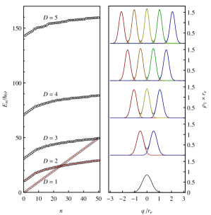
Figure 1: (Color online) Left: Energy spectrum for $D$ LJ particles in a 1D harmonic trap obtained with our method (circles). The exact results for $D=1$ and $2$ are shown as red solid lines. Energies are shifted to the minimum of the potential $\min(\mathcal{H}_{1})=-\epsilon(D-1)D/2$. Right: One-body densities (normalized to the number of particles) of the ground state for distinguishable (colored lines) and indistinguishable particles (black lines).

As a more stringent test, we now apply the method to $D$ LJ particles in a one-dimensional harmonic trap. Potentials $V_{1}$ and $V_{2}$ are defined by

$$V_{1}({\mathbf{q}}) =\sum_{\lambda=1}^{D}\frac{1}{2}m\omega^{2}q_{\lambda}^{2},$$ (12)

$$V_{2}({\mathbf{q}}) =\sum_{\lambda<\mu}^{D}V_{\mathrm{LJ}}(|q_{\lambda}-q_{\mu}|),$$ (13)

the de Boer length has the same value as in the example above, and $\omega r_{e}\sqrt{m/\epsilon}=1/2$. The problem is separable only for $D=1$ or $2$, and so a multidimensional numerical method is mandatory for $D\geq 3$. In order to reduce the number of grid points in the numerical calculation, we first solve the problem for distinguishable particles and construct a posteriori the eigenstates of indistinguishable particles by symmetrizing or anti-symmetrizing the wavefunction for spinless bosons or fermions, respectively. Thanks to the repulsive nature of the LJ potential at short distances we only need to evaluate $\hat{K}$ in the subspace defined by $q_{1}>q_{2}+a,\dots,$ $q_{D-1}>q_{D}+a$, where $a$ is the core radius of the LJ potential, within which the wavefunction is expected to be zero within numerical accuracy ($a=0.63r_{e}$ in our calculations). The grid points are sampled from the classical Boltzmann distribution of the harmonic trap in this subspace, $p({\mathbf{q}})=Z_{V_{1}}^{-1}e^{-\Delta\tau m\omega^{2}|{\mathbf{q}}|^{2}/2\hbar}$ with $Z_{V_{1}}=(2\pi/\Delta\tau m\omega^{2})^{D/2}/C_{D}(a)$, where the normalization constant obeys $C_{D}(0)=D!$. All the two-body interactions, contained in $V_{2}({\mathbf{q}})$, are evaluated in the matrix elements of $\hat{K}$. As mentioned above, only the low-lying eigenstates are accurate, so we have used the Arnoldi algorithm Arnoldi (1951) to obtain the first 50 eigenstates. We have taken into account that many of the matrix elements are close to zero by using standard computational techniques for sparse matrices: instead of storing the $N\times N$ values of the matrix, only elements larger than a certain threshold were stored. Parameters used in calculations with varying $D$ were

$$\begin{array}[c]{r|ccccc}D&1&2&3&4&5\\ \hline\cr N&500&6709&14\leavevmode\nobreak\ 394&36\leavevmode\nobreak\ 517&84\leavevmode\nobreak\ 690\\ \Delta\tau&0.0055&0.15&1.5&1.5&1.5\end{array}$$

Note the relatively low total number of grid points needed to obtain results with reasonable accuracy (a relative error of 0.002 for the $D=2$ case). Figure 2 shows the ground and 19th states for $D=2$ and for the three statistics: distinguishable particles (in the above mentioned subspace), bosons, and fermions (in the full space). The spectrum of $\mathcal{H}$ as a function of $D$ is shown in Fig. 1 (left panel). We find the same spectrum for the three cases, which is a consequence of the fermionization Paredes et al. (2004) mechanism due to the repulsive behavior of the LJ potential at short distances. Indeed, the bosonic and fermionic systems show the same one-body densities in position space, as shown in the right panel of Fig. 1. In all three cases the densities show a well-defined structure, forming a quantum crystal. The displayed one-body densities, defined as Lipparini (2008)

$$\rho_{n}(q_{\lambda})=\int|\varphi_{n}({\mathbf{q}})|^{2}\prod_{\mu\neq\lambda}^{D}dq_{\mu},$$ (14)

were obtained from the nonuniform mesh as follows: first,we computed its Fourier transform in a regular equidistant grid in momentum ($k$) space as

$$\tilde{\rho}_{n}(k) =\int|\varphi_{n}({\mathbf{q}})|^{2}e^{-ikq_{\lambda}}\prod_{\mu=1}^{D}dq_{\mu}$$ (15)

$$\approx\frac{Z}{N}\sum_{j=1}^{N}e^{\Delta\tau V_{1}({\mathbf{q}}_{j})/\hbar-ikq_{\lambda}}|\varphi_{n}({\mathbf{q}}_{j})|^{2},$$ (16)

and then Fourier-transformed $\tilde{\rho}_{n}(k)$ back to $q_{\lambda}$-space using standard numerical methods.

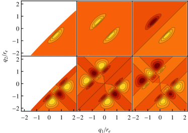
Figure 2: (Color online) Wavefunctions $\varphi_{n}(q_{1},q_{2})$ of the ground and 19th states for $D=2$ LJ particles in a 1D harmonic trap (see text for details). Lighter (darker) color indicates positive (negative) values of the wavefunction. Left: distinguishable particles in the subspace $q_{1}>q_{2}$; center: indistinguishable bosons; right: indistinguishable fermions.

The 50 states obtained in the course of the diagonalization are sufficient to study the behavior of the system at finite temperatures. The (unnormalized) probability distribution of the system $p_{\beta}({\mathbf{q}})$ at finite inverse temperature $\beta$ is defined as the thermal average

$$p_{\beta}({\mathbf{q}})=\sum_{n=1}^{\infty}e^{-\beta E_{n}}|\varphi_{n}({\mathbf{q}})|^{2},$$ (17)

and the corresponding one-body density $\rho_{\beta}(q)$ is obtained similarly as for pure states. Figure 3 shows the one-body density for $D=4$ at three different temperatures, where the lack of structure at the highest temperature can be understood as the melting of the quantum crystal.

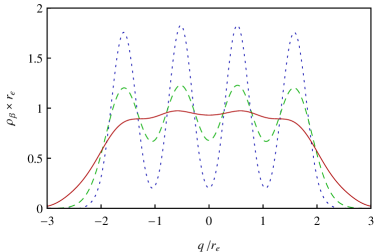
Figure 3: (Color online) One-body densities (normalized to the number of particles) for $D=4$ LJ particles in a 1D harmonic trap at three different temperatures: $\hbar\omega\beta=2.8$ (dotted line), $0.7$ (dashed line), and $0.4$ (solid line). The crystal structure disappears with increasing temperature, resulting in an unstructured total density as in a fluid.

To summarize, we have presented compelling evidence that the proposed method achieves the original goals. Indeed, (i) the only approximation used is the numerical discretization of space and time; (ii) the ITNUMM only requires standard methods for sampling from an arbitrary probability distribution and for diagonalizing real-valued sparse matrices; (iii) both ground and excited states are obtained in the course of the diagonalization; and (iv) due to the nonuniform nature of the grid that uses the potential to guide the sampling, the complexity of the algorithm is significantly reduced in high-dimensional systems. In particular, all our calculations were performed on a single workstation with a 64-bit 2.4 GHz Quad-Core Intel Xeon E5 processor and 12 GB of memory. Yet, the algorithm can be easily accelerated by parallelization. The accuracy of ITNUMM can be increased by using tailored grids, larger $N$ values, or splitting methods of a higher order than in Eq. (3). In addition to computing thermal averages—as shown here—the large set of excited states can be also used for solving real-time quantum dynamics in a straightforward fashion. As we have not found any a priori limitation to the applicability of the method, other systems described by the MDSE will be studied in the future.

Acknowledgments. The authors thank E. Zambrano, M. Wehrle, M. Šulc, and F. Mazzanti for discussions. This research was supported by the Swiss NSF NCCR MUST (Molecular Ultrafast Science & Technology) and by the EPFL.

References

- Harris et al. (1965) D. O. Harris, G. G. Engerholm, and W. D. Gwinn, J. Chem. Phys. 43, 1515 (1965).
- Kosloff (1988) R. Kosloff, J. Phys. Chem. 92, 2087 (1988).
- Shimshovitz and Tannor (2012) A. Shimshovitz and D. J. Tannor, Phys. Rev. Lett. 109, 070402 (2012).
- Pollet (2012) L. Pollet, Rep. Prog. Phys. 75, 094501 (2012).
- Parr and Yang (1994) R. G. Parr and W. Yang, Density-Functional Theory of Atoms and Molecules, 2 ed. (Oxford University Press, 1994).
- Dalfovo et al. (1995) F. Dalfovo, A. Lastri, L. Pricaupenko, S. Stringari, and J. Treiner, Phys. Rev. B 52, 1193 (1995).
- Savenko et al. (2013) I. G. Savenko, T. C. H. Liew, and I. A. Shelykh, Phys. Rev. Lett. 110, 127402 (2013).
- Rogel-Salazar (2013) J. Rogel-Salazar, Eur. J. Phys. 34, 247 (2013).
- Billing and Adhikari (2000) G. Billing and S. Adhikari, Chem. Phys. Lett. 321, 197 (2000).
- Runge and Gross (1984) E. Runge and E. K. U. Gross, Phys. Rev. Lett. 52, 997 (1984).
- Abid et al. (2003) M. Abid, C. Huepe, S. Metens, C. Nore, C. T. Pham, L. S. Tuckerman, and M. E. Brachet, Fluid Dyn. Res. 33, 509 (2003).
- Wyatt and Trahan (2005) R. E. Wyatt and C. J. Trahan, Quantum Dynamics with Trajectories: Introduction to Quantum Hydrodynamics, 1st ed. (Addison-Wesley, 2005).
- Alvarez et al. (2011) G. Alvarez, L. G. G. V. D. da Silva, E. Ponce, and E. Dagotto, Phys. Rev. E 84, 056706 (2011).
- Tkatchenko et al. (2012) A. Tkatchenko, R. A. DiStasio, R. Car, and M. Scheffler, Phys. Rev. Lett. 108, 236402 (2012).
- Martín-Delgado and Sierra (1996) M. A. Martín-Delgado and G. Sierra, Phys. Rev. Lett. 76, 1146 (1996).
- Corney and Drummond (2004) J. F. Corney and P. D. Drummond, Phys. Rev. Lett. 93, 260401 (2004).
- Torres-Vega and Frederick (1991) G. Torres-Vega and J. H. Frederick, Phys. Rev. Lett. 67, 2601 (1991).
- McMahon et al. (2012) J. M. McMahon, M. A. Morales, C. Pierleoni, and D. M. Ceperley, Rev. Mod. Phys. 84, 1607 (2012).
- Kapitza (1938) P. Kapitza, Nature 141, 74 (1938).
- Leggett (1972) A. J. Leggett, Phys. Rev. Lett. 29, 1227 (1972).
- Grebenev et al. (2000) S. Grebenev, B. Sartakov, J. P. Toennies, and A. F. Vilesov, Science 289, 1532 (2000).
- Anglin and Ketterle (2002) J. R. Anglin and W. Ketterle, Nature 416, 211 (2002).
- Balibar (2010) S. Balibar, Nature 464, 176 (2010).
- Bloch (2005) I. Bloch, Nature Physics 1, 23 (2005).
- Ronzheimer et al. (2013) J. P. Ronzheimer, M. Schreiber, S. Braun, S. S. Hodgman, S. Langer, I. P. McCulloch, F. Heidrich-Meisner, I. Bloch, and U. Schneider, Phys. Rev. Lett. 110, 205301 (2013).
- Panfil et al. (2013) M. Panfil, J. D. Nardis, and J.-S. Caux, Phys. Rev. Lett. 110, 125302 (2013).
- Vignolo and Minguzzi (2013) P. Vignolo and A. Minguzzi, Phys. Rev. Lett. 110, 020403 (2013).
- Gring et al. (2012) M. Gring, M. Kuhnert, T. Langen, T. Kitagawa, B. Rauer, M. Schreitl, I. Mazets, D. A. Smith, E. Demler, and J. Schmiedmayer, Science 337, 1318 (2012).
- Kinoshita et al. (2006) T. Kinoshita, T. Wenger, and D. S. Weiss, Nature 440, 900 (2006).
- Paredes et al. (2004) B. Paredes, A. Widera, V. Murg, O. Mandel, S. Folling, I. Cirac, G. V. Shlyapnikov, T. W. Hansch, and I. Bloch, Nature 429, 277 (2004).
- Bloch et al. (2008) I. Bloch, J. Dalibard, and W. Zwerger, Rev. Mod. Phys. 80, 885 (2008).
- Morton and Mayers (2005) K. Morton and D. Mayers, Numerical Solution of Partial Differential Equations, An Introduction, 2 ed. (Cambridge University Press, 2005).
- Popov (2005) V. S. Popov, Phys. Atom. Nuclei 68, 686 (2005).
- Sakurai (1993) J. J. Sakurai, Modern Quantum Mechanics , 1 ed. (Addison-Wesley, 1993).
- Deckman and Mandelshtam (2009) J. Deckman and V. A. Mandelshtam, J. Phys. Chem. A 26, 7394 (2009).
- Arnoldi (1951) W. E. Arnoldi, Q. Appl. Math 9, 17 (1951).
- Lipparini (2008) E. Lipparini, Modern Many-Particle Physics: Atomic Gases, Nanostructures and Quantum Liquids (World Scientific, 2008).