Accepted for publication in Sol. Phys. - 2013

  
¹ Physical Research Laboratory, Ahmedabad - 380009, India.
email: susanta@prl.res.in email: jerry@prl.res.in

² Physical Research Laboratory, Space & Atmospheric Sciences Division,
Ahmedabad - 380009, India. email: dipu@prl.res.in

³ Electronic Science Department, Pune University, Pune 411 007, India.
email: subra.anan@gmail.com e-mail: wiztronix@gmail.com

abstract

Using both wavelet and Fourier analysis, a study has been undertaken of the changes in the quasi-periodic variations in solar photospheric fields in the build-up to one of the deepest solar minima experienced in the past 100 years. This unusual and deep solar minimum occurred between solar cycles 23 and 24. The study, carried out using ground based synoptic magnetograms spanning the period 1975.14 to 2009.86, covered solar cycles 21, 22 and 23. A hemispheric asymmetry in periodicities of the photospheric fields was seen only at latitudes above $\pm$45^∘ when the data was divided, based on a wavelet analysis, into two parts: one prior to 1996 and the other after 1996. Furthermore, the hemispheric asymmetry was observed to be confined to the latitude range 45^∘ to 60^∘. This can be attributed to the variations in polar surges that primarily depend on both the emergence of surface magnetic flux and varying solar surface flows. The observed asymmetry when coupled with the fact that both solar fields above $\pm$45^∘ and micro-turbulence levels in the inner-heliosphere have been decreasing since the early to mid nineties (Janardhan et al., 2011) suggests that around this time active changes occurred in the solar dynamo that governs the underlying basic processes in the sun. These changes in turn probably initiated the build-up to the very deep solar minimum at the end of the cycle 23. The decline in fields above $\pm$45^∘ for well over a solar cycle, would imply that weak polar fields have been generated in the past two successive solar cycles viz. cycles 22 and 23. A continuation of this declining trend beyond 22 years, if it occurs, will have serious implications on our current understanding of the solar dynamo.

Introduction

The delayed onset of solar cycle 24, after one of the deepest solar minimum experienced in the past 100 years has had significant solar and heliospheric consequences. Solar cycle 23 has been characterized by a steady decline in solar activity (McComas et al., 2008; Jian, Russell, and Luhmann, 2011), a continuous weakening of polar fields (Jiang et al., 2011) and a decline in micro-turbulence levels in the inner heliosphere since $\sim$1995 (Janardhan et al., 2011). Investigations of the boundary of polar coronal holes during the declining phase of solar cycle 23 using images from the Extreme Ultraviolet Imaging Telescope (EIT) on board the Solar Heliospheric Observatory (SoHO), have found a decrease in coronal hole area by $\sim$15$\%$ in comparison to that at the beginning of solar cycle 23 (Kirk et al., 2009). Using both ground-based and space-borne observations of photospheric magnetic fields (Janardhan, Bisoi, and Gosain, 2010; Hathaway and Rightmire, 2010) and theoretical modeling (Dikpati et al., 2010; Nandy, Muñoz-Jaramillo, and Martens, 2011), there have been continuous efforts to investigate and understand the behavior of solar photospheric fields and their correlation with meridional flows, to try and explain the delayed onset of cycle 24 and the cause of the deep minimum at the end of cycle 23.

Magnetic field measurements using data from the National Solar Observatory, Kitt Peak (NSO/KP) synoptic magnetogram database, have shown that a decline in solar photospheric fields in the latitude range 45^∘ to 78^∘ began around the minimum of solar cycle 22, in $\sim$1995$-$1996 (Janardhan, Bisoi, and Gosain, 2010). However, the dipole field of the Sun behaved differently. It was at its strongest in 1995, weakened at solar maximum around 2000, and then increased between $\sim$2000 and 2004 (Wang, Robbrecht, and Sheeley, 2009; Janardhan, Bisoi, and Gosain, 2010). Signatures of this decline in solar fields above latitude $\pm$45^∘ have also been observed in the inner heliosphere as a corresponding decline in micro-turbulence levels which in turn, tie into small scale interplanetary magnetic fields (Ananthakrishnan, Coles, and Kaufman, 1980; Ananthakrishnan, Balasubramanian, and Janardhan, 1995). The decline in micro-turbulence levels was inferred from extensive interplanetary scintillation (IPS) observations at 327 MHz in the period 1983$-$2009 (Janardhan et al., 2011). Using this fact viz. that both solar magnetic fields and micro-turbulence levels in the inner-heliosphere have been declining since mid 1990’s, Janardhan et al. (2011) have argued that the build-up to the deep and extended solar minimum at the end of cycle 23 was actually initiated as early as the mid-1990’s.

One method of gaining insights into underlying basic processes in the solar interior, that govern the nature and evolution of solar photospheric magnetic fields, is by studying periodicities produced by various surface activity features at different times in the solar cycle. For example, the 158 days (d) Rieger periodicity reported in the solar flare occurrence rates (Oliver, Ballester, and Baudin, 1998) has been linked to the periodic emergence of magnetic flux through the photosphere which in turn gives rise to a periodic variation of the total sunspot area on the solar surface. Similarly, a strong 1.3 years (yr) periodicity detected at the base of the solar convection zone, through a helioseismic study (Howe et al., 2000), has also been detected in sunspot areas and sunspot number time series studied using wavelet transforms (Krivova and Solanki, 2002). These authors have in fact proposed that the 154${-}$158 d Rieger period is a harmonic of the 1.3 yr periodicity (3$\times$156 d = 1.28 yr) and that variations in the rotation rate have a strong influence on the workings of the solar dynamo (Krivova and Solanki, 2002).

In this paper, in order to understand the role of periodic changes, if any, in the solar photospheric fields leading to the build-up of the recent deep minimum at the end of cycle 23, data from the NSO/KP synoptic magnetic database during the period 1975.14 $-$ 2009.86 were subjected to detailed spectral analyses using both wavelet and Fourier techniques. It has been shown that a significant north-south asymmetry in the quasi-periodic variations of the photospheric magnetic fields exist both prior to and after 1996 (with 1996 being a clear transition period) almost 12 yr before the deep minimum period in 2008$-$2009.

Solar Periodicities

Prominent periodicities related to the solar cycle, apart from the well known synodic rotation period of $\sim$27 d and the sunspot activity cycle of $\sim$11 yr, have been a topic of interest for over two decades now. Using data from the Gamma Ray Spectrometer (Forrest et al., 1980) onboard the Solar Maximum Mission, a clear 154 d periodicity in the occurrence rate of high energy (0.3-100 MeV) flares has been reported (Rieger et al., 1984). This 154 d periodicity in the solar flare occurrence was also confirmed at other wavelengths (Verma and Joshi, 1987; Droege et al., 1990; Kile and Cliver, 1991; Chowdhury and Ray, 2006), and for solar energetic particle events (Lean, 1990; Krivova and Solanki, 2002; Kiliç, 2008; Chowdhury, Khan, and Ray, 2010; Chowdhury and Dwivedi, 2011).

In addition, other intermediate periodicities with periods ($<$1 yr) have also been reported viz. a 51 d periodicity in the comprehensive flare index (Bai, 1987), a 127 d periodicity in the 10 cm radio flux (Kile and Cliver, 1991), periodicities of 33.5 d, 51 d, 84 d, 129 d and 153 d in the solar flare occurrence during different phases of solar cycles 19$-$23 (Bai, 2003), periodicities of 100$-$103 d, 124$-$129 d, 151$-$158 d, 177$\pm$2 d, 209$-$222 d, 232$-$249 d, 282$\pm$4 d, 307$-$349 d in the unsigned photospheric fluxes (Knaack, Stenflo, and Berdyugina, 2005) and periodicities of 87-106 d, 159-175 d, 194-219 d, 292$-$318 d, and 69$-$95 d, 113$-$133 d, 160$-$187 d, 245$-$321 d, 348$-$406 d in sunspot areas at different phases of cycle 22 and 23 respectively (Chowdhury, Khan, and Ray, 2009).

For periodicities, between 1$-$5 yr, a 1.3 yr periodicity in sunspot areas and numbers (Krivova and Solanki, 2002), 1 yr and 1.7 yr periodicity in solar total and open fluxes (Mendoza, Velasco, and Valdés-Galicia, 2006), 1.3 yr, 1.43 yr, 1.5 yr, 1.8 yr, 2.4 yr, 2.6 yr, 3.5 yr, 3.6 yr and 4.1 yr in unsigned photospheric fluxes (Knaack, Stenflo, and Berdyugina, 2004, 2005) have been reported. Studies of all these periodicities have shown the existence of an asymmetry in solar activity phenomena between the northern and southern hemispheres of the sun. This hemispheric asymmetry, on different time scales and at different phases of different solar cycles, have been observed in various types of solar activity (Howard, 1974; Verma, 1987; Oliver and Ballester, 1994; Knaack, Stenflo, and Berdyugina, 2005) and have been providing invaluable information about basic underlying physical processes on the sun. Since processes like differential rotation of the sun and emergence of magnetic flux determine the strength and distribution of solar magnetic activity, investigation of solar cycle related periodic or quasi-periodic variations is crucial in understanding the behavior and nature of solar magnetic fields.

Decline in mid to high latitude solar fields

Figure 1 shows temporal variation in the unsigned or absolute solar photospheric magnetic fields in the latitude range, 45^∘$-$78^∘ in both solar hemispheres, for the period from February 1975 to November 2009 (panel a) covering solar cycles 21, 22, and 23. The vertically oriented dotted lines demarcate the period of solar minimum of these three solar cycles. The small, black filled dots and the open circles are the actual measurements for the northern and southern hemispheres respectively while the solid red (northern hemisphere) and blue (southern hemisphere) lines are smoothed curves derived using a robust Savitzky-Golay (SG) algorithm (Savitzky and Golay, 1964) that has the ability to preserve features of the input distribution like maxima and minima while effectively suppressing noise. Such features are generally flattened by other smoothing techniques. The decline in photospheric magnetic fields in both hemispheres, starting around the early to mid-1990’s can be clearly seen in Fig. 1. While the decline in photospheric fields had started in $\sim$1991 for the northern hemisphere (solid red curve), for the southern hemisphere the decline started in $\sim$1995 (solid blue curve). Beyond $\sim$1996, a steady decline in the photospheric fields for both hemispheres can be clearly seen. A similar decline in the sunspot umbral magnetic field strength since $\sim$1998 has also been reported (Livingston, 2002; Penn and Livingston, 2006). Also shown in the bottom two panels of Fig. 1 are the magnetic residuals, obtained by subtracting the SG fit from the actual measurements, for both the hemispheres in the latitude range 45^∘$-$78^∘ (panel b) and 0^∘$-$45^∘ (panel c) respectively. See the upper two panels of Fig. 1 in Janardhan, Bisoi, and Gosain (2010) for measurements of the magnetic field in the range $\pm$45^∘ which show a strong solar cycle modulation in the data as expected.

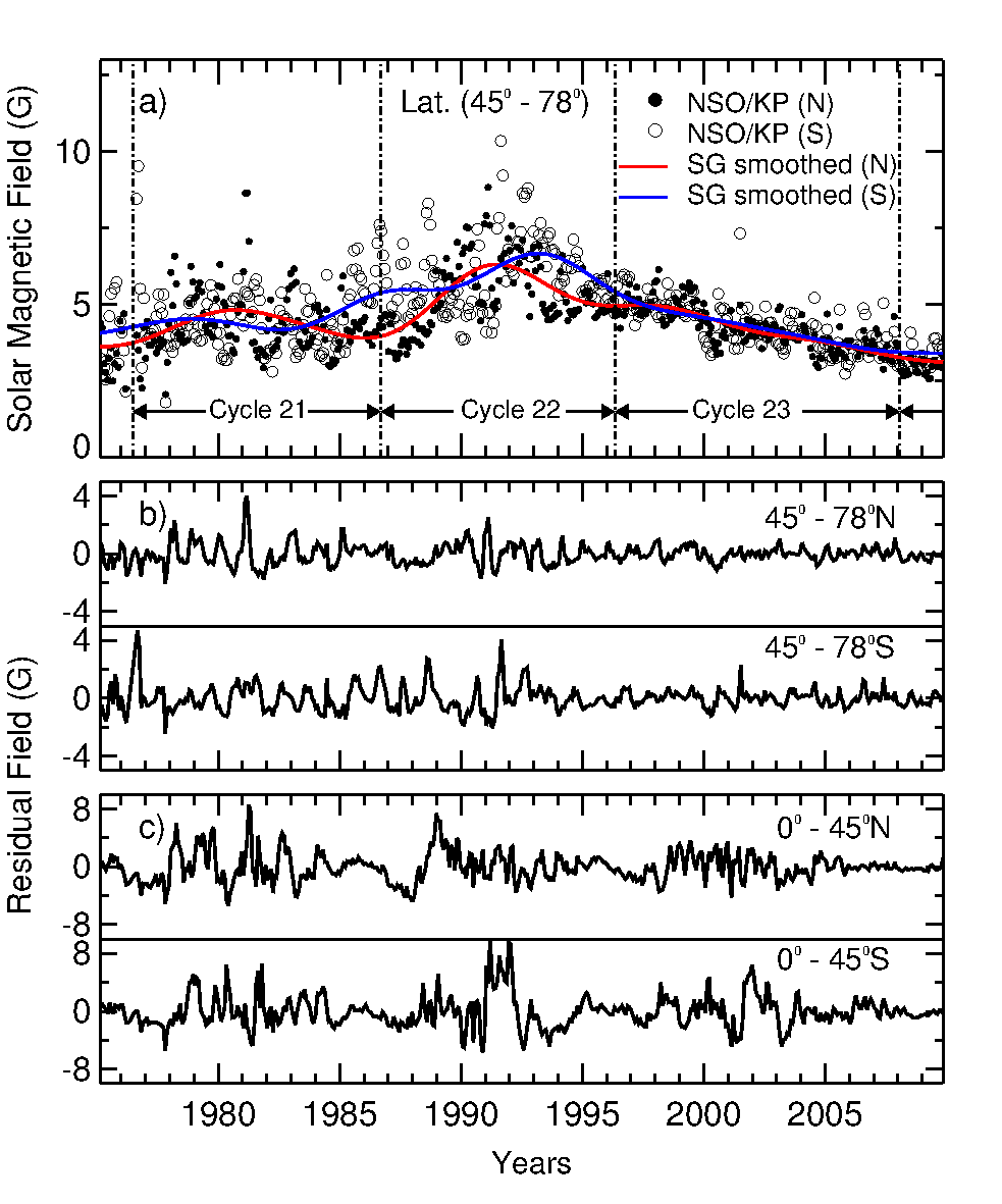
Figure 1: a) Shows measurements of solar photospheric magnetic fields in the latitude range, 45^∘ to 78^∘. The filled dots and the open circles respectively represent the actual measurements for the northern and southern hemispheres while the fit obtained using the SG algorithm is shown by the solid red (north) and blue (south) lines. The vertically oriented dotted lines demarcate the periods of solar cycles 21, 22 and 23. b) The residuals obtained after subtracting the SG smoothed values from the magnetic fields in the latitude range, 45^∘ to 78^∘, are shown for the north and south. c) Show the residual fields for both the northern and southern hemispheres obtained from the magnetic fields at latitudes below 45^∘.

Brief details of the method by which the magnetic fields were derived are given below. We have used measurements of magnetic field strengths obtained from 466 individual Carrington rotations (CR) of NSO/KP synoptic magnetograms from CR1625 through CR2090 in the period from 19 February 1975 to 09 November 2009 (1975.14$-$2009.86). Each magnetogram, generated from daily ground-based full-disk magnetograms spanning over a Carrington rotation period corresponding to 27.27 days, was longitudinally averaged to a 1^∘ wide longitudinal strip covering the latitude range from -90^∘ to +90^∘. Surface magnetic fields in both equatorial (-45^∘ to +45^∘) and high-latitude zones ($>$45^∘ in both hemispheres) of the sun were then derived by averaging over appropriate latitude regions. Full details of the method used are described in Janardhan, Bisoi, and Gosain (2010).

The SG smoothing is done in such a way as to make the resulting residual time series stationary i.e. the mean of time series is or approaches zero. Such a detrending of the data removes large periodic variations ($\sim$11 years). The residuals were then subjected to both a wavelet analysis and a Fourier time series analysis to study temporal periodic variations in photospheric magnetic fields. In the rest of the text the fields obtained in the equatorial belt of -45^∘ to +45^∘ are referred to as low-latitude fields while the fields obtained at latitudes $>$45^∘ in both hemispheres are referred to as high-latitude fields.

Transition in Wavelet Periodicities

A wavelet transform is basically the convolution of a time series with the scaled and translated version of a chosen “mother” wavelet function. The wavelet analysis now finds frequent use in the analysis of time series data since it yields information in both time and frequency domains (Torrence and Compo, 1998). Using a Morlet wavelet as the mother wavelet and based on the algorithm by Torrence and Compo (1998), the magnetic residuals obtained for both the high-latitude and low-latitude fields in the period from 19 February 1975 to 09 November 2009 (1975.14$-$2009.86) were subjected to a wavelet analysis. Scattered data gaps amounting to $\sim$ 2.5% of the data were replaced with values obtained using a cubic spline interpolation. The Morlet wavelet function $\psi_{0}(\eta)$, represented in equation 1 below, is a plane wave modulated by a Gaussian.

$$\mathsf{\psi_{0}(\eta)=\pi^{-1/4}e^{i\omega_{0}\eta}e^{-\eta^{2}/2}}$$ (1)

Here, $\omega_{0}$ is a non-dimensional frequency that determines the number of oscillations in the wavelet and $\eta$ is a non-dimensional time parameter. The choice of different non-dimensional frequencies defines the frequency resolution. However, by varying the frequency resolution, one has to compromise with time resolution. In this case, we have chosen $\omega_{0}$ to be 6 for obtaining a better frequency resolution. This value is left unchanged and is not tuned to different values as our interest is to look for changes in the frequency components rather than to find precisely the low and high frequency components. However, in the following sections, we have employed a Fourier analysis technique to find the various frequency components.

Figure 2 shows the wavelet spectrum for the high-latitude fields in the northern (upper panel) and southern hemisphere (lower panel) while Figure 3 shows the wavelet spectrum for the low-latitude fields in the northern (upper panel) and southern hemispheres (lower panel). The green cross-hatched regions in both figures represent the cone of influence (COI) where the spectral distribution is not reliable. The white contours are drawn at a significance level of 95%. The power levels are indicated by a color coded bar on the right of each panel and the dashed vertical line in each panel is drawn at 1996 in both Figures 2 and 3. For the high-latitude fields (Fig. 2), in both the north and south, significant wavelet power is only seen at lower periods ($\sim$1$-$3 yr) prior to 1985 while significant wavelet power is seen both at lower and higher periods ($\sim$3$-$5 yr) for the interval between 1985 and 1996. For the low-latitude fields (Fig. 3), we don’t see significant changes in the power levels between 1975 and 1996.

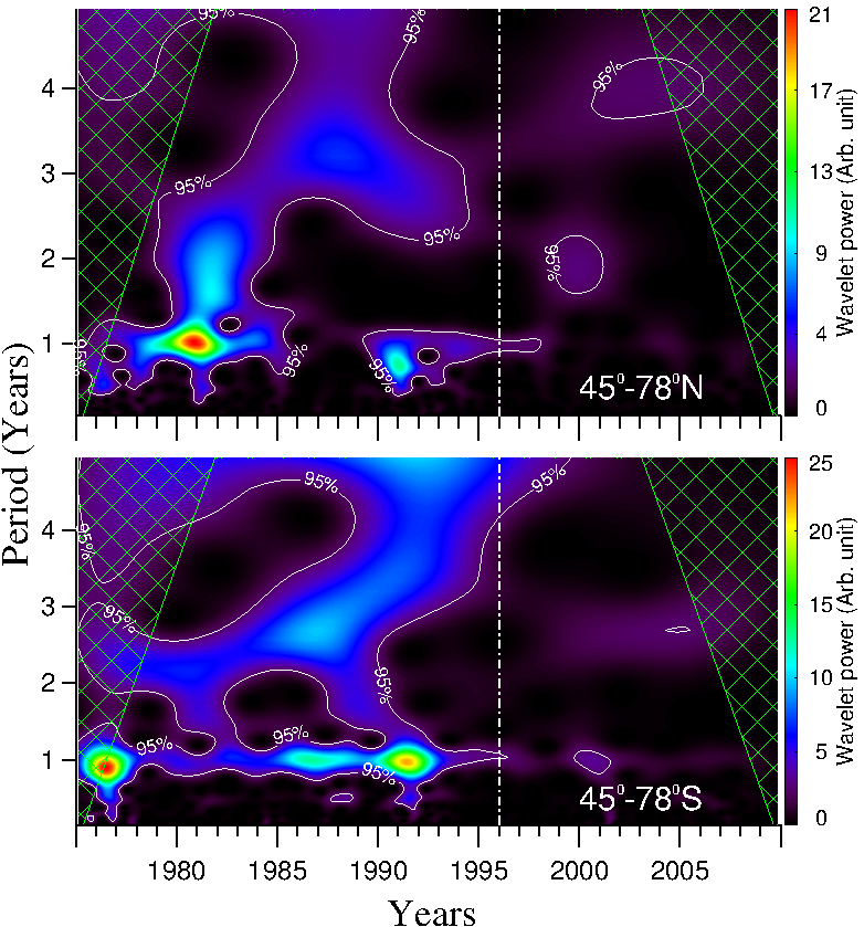
Figure 2: Shows the wavelet power distribution of solar periodicity over years for high-latitude fields for the northern hemisphere (upper panel) and southern hemisphere (lower panel) in the latitude range, 45^∘ to 78^∘. The green cross hatched regions are the cone of influence (COI) while the white contours indicate a significance level at 95%. The dashed vertical lines are marked at 1996 when a clear transition has observed in wavelet power of periodicities for both the north and south high-latitude fields.

It is important to note here that there is a clear transition in both periodicities and power levels in both hemispheres around 1996 for both high-latitude and low-latitude fields. We stress here that we have taken care to check that the selection of different colors or changes in the color intensity in the wavelet plots makes no difference in the transition noticed in the wavelet power spectra. Though the decline in the fields has started in the early to mid 1990’s, as seen from Fig. 1, we see from the wavelet spectra that there is an unambiguous transition in the quasi-periodic variations of fields in both the hemispheres at $\sim$1996. We have therefore chosen, in the rest of the analysis, to divide the residuals into two sets based on this transition seen in the wavelet spectra around $\sim$1996 in order to study the changes, if any, in the periodicities before and after the transition seen in the wavelet spectra. A Fourier time series analysis was then carried out separately on the residuals used in the wavelet analysis for the period prior to 1996 and the period after 1996 for both high-latitude and low-latitude fields.

It is important to bear in mind here that the transition seen in the wavelet spectra around 1995$-$1996 corresponds to the time when both solar high-latitude fields above $\pm$45^∘ and solar wind turbulence levels in the entire inner-heliosphere began declining (Janardhan, Bisoi, and Gosain, 2010; Janardhan et al., 2011).

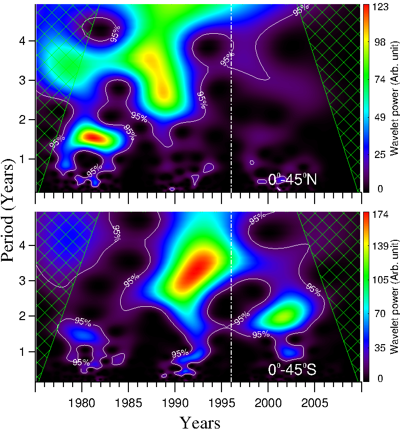
Figure 3: Shows the wavelet power distribution of solar periodicity over years for low-latitude fields for the northern hemisphere (upper panel) and southern hemisphere (lower panel) in the latitude range, 0^∘ to 45^∘. The green cross hatched regions are the cone of influence (COI) while the white contours indicate a significance level at 95%. The dashed vertical line demarcates the period of transition in wavelet power of periodicities for both the hemispheres around 1996.

Fourier periodicities - Asymmetries and symmetries

Based on the transition seen in the wavelet spectra at $\sim$1996, we have subjected the residuals obtained from the SG fits to a Fourier analysis after dividing the time series of the residuals, spanning years 1975.14 to 2009.86, into two parts, one prior to 1996 and the other after 1996. Since the time series of the residual field has some data gaps amounting to $\sim$2.5% of the data, the algorithm used for this purpose was based on the Lomb-Scargle Fourier Transform for unevenly spaced data (Lomb, 1976; Scargle, 1982, 1989; Schultz and Stattegger, 1997) in combination with the Welch-Overlapped-Segment-Averaging (WOSA) procedure (Welch, 1967). The spectral power derived from such an analysis is generally normalized with respect to the total power contained in all the Fourier components taken together. This procedure makes the relative distribution of the spectral power independent of the spectral windowing used in the algorithm. Such normalized power spectra are referred to as normalized Fourier periodograms or simply normalized periodograms.

High-latitude Fields

Normalized periodograms obtained from the Fourier analysis are shown in Figure 4. The top four panels of Fig. 4 labeled a, b, c and d represent the high-latitude fields while the bottom four panels of Fig. 4 labeled e, f, g, and h represent the low-latitude fields. The upper four panels (high-latitude fields) show normalized periodograms before and after 1996 in the north (panels a and b respectively), and before and after 1996 in the south (panels c and d respectively). In a similar fashion, the lower four panels (low-latitude fields) show normalized periodograms in the north before and after 1996 (panels e and f respectively) and in the south before and after 1996 (panels g and h respectively). The “${significant}$” periodic components were determined using the Siegel test statistics (Siegel, 1980) and are those components having power levels above the black horizontal line drawn in each panel of Fig. 4. The Siegel’s test is an extension of the Fisher’s test (Fisher, 1929). While Fisher’s test attempts to spot the single dominant periodicity in a time series that has maximum power in the periodogram and is above the “${critical}$” level defined by Fisher’s test statistics, Siegel’s test (Siegel, 1980) relaxes this stringent condition a little and considers two to three dominant periodic components above the “${critical}$” level. Both the aforementioned test statistics and the process of determining the confidence/significance level are discussed in (Percival and Walden, 1993) and also briefly in (Schultz and Stattegger, 1997). In the present analysis, 95% confidence level (or 5% significance level) is chosen. This is equivalent to $\pm$2$\sigma$ level in FFT method. It is to be noted that the choice of this confidence level decides the “${critical}$” level of the Sigel test statistics (Schultz and Stattegger, 1997).

It may be noted that though the Fourier components obtained from the analysis range in periods from 54 d to 12 yr corresponding to 214 nHz to 2.6 nHz in frequency, Fig. 4 only shows those components with periods lying in the range 300 d to 12 yr ${\it{i.e.}}$ the low-frequency range. Normalized periodograms containing Fourier components with periods less than 300 d will be discussed later.

The red vertical lines in each panel of Fig. 4 are drawn through the peak of the component with the longest period. A shift in the periodicities can be seen after 1996 when compared to that before 1996. This shift is indicated by vertical dashed blue lines and a black arrow showing the direction of the shift in periodicities. It must be emphasized that we are not interested in the actual periodicities themselves but rather in the manner in which the longest periodicities shift between the time interval prior to and after 1996. It can be seen from Fig. 4 that in addition to the shift in periodicity of the high-latitude fields in both hemispheres before and after 1996 the spectral power also differs significantly before and after 1996. The longer periods after 1996 have more spectral power than longer periods prior to 1996. If we denote the longest periods for the high-latitude fields in the north before 1996 as $T_{1}$ and that after 1996 as $T_{2}$, we find that $T_{2}$ $>$ $T_{1}$ for high-latitude fields in the north.

For the southern hemisphere, the direction of the shift in periodicities, as indicated by the direction of the black arrow in Fig. 4, is in the opposite direction as compared to the northern hemisphere. If we denote the longest periods for the high-latitude fields in the south before 1996 and after 1996 as $T_{3}$ and $T_{4}$ respectively, we find that $T_{4}$ $<$ $T_{3}$ for the high-latitude fields in the south. As in the case of the northern hemisphere, the distribution of spectral power in various periodicities is also significantly different in the periods before and after 1996.

Thus, a north-south asymmetry is seen in the distribution of periodicities for the high-latitude fields along with significant changes in the power of various periodic components. Since the normalized periodograms are generated from measurements of magnetic fields, it is a proxy for the behaviour of the photospheric magnetic fields and a north-south asymmetry would imply a similar asymmetry in photospheric magnetic fields towards higher solar latitudes before and after 1996.

Low-latitude fields

In contrast to the behavior of the high-latitude fields, the low-latitude fields represented in the bottom four panels of Fig. 4 and labeled e, f, g and h show no asymmetry in the manner in which the longest periods shift when one compares the periodograms prior to and after 1996. The shift in the longest periods in both the north and south low-latitude fields before and after 1996 has been depicted in the lower four panels of Fig. 4 in a similar fashion to that of the upper four panels. The vertical solid red line is drawn through the peak of the component with the longest period and the dotted blue line and a black arrow in each panel indicate the direction of the shift.

Denoting the longest period for the low-latitude fields in the north before and after 1996 as $T_{5}$ and $T_{6}$ respectively, we find that $T_{5}$ $>$ $T_{6}$. In the southern hemisphere, denoting the longest period for the low-latitude fields prior to 1996 and after 1996 as $T_{7}$ and $T_{8}$ respectively, it is clear that $T_{7}$ $>$ $T_{8}$. Hence, the longest periods show a shift in the same direction indicating no asymmetry in the distribution of the low-latitude fields before and after 1996.

Figure 4: The top four panels - a, b, c, d and the bottom four panels - e, f, g, h respectively represent normalized Fourier periodograms for high-latitude fields and low-latitude fields. The four panels in the top and the bottom show respectively, the normalized Fourier power distribution with periodicity for photospheric fields in the north before 1996, in the north after 1996, in the south before 1996 and in the south after 1996. The solid red vertical lines demarcate the highest period in each of the four panels while the dotted blue vertical line and direction of the black arrow in each panel are used to show the shift in the periodicity of the longest periods. The solid horizontal lines depict significance levels as determined by Siegel test. The new periodicities from our analysis have been boxed in blue.

Latitudinal profile for Fourier power spectrum

To examine how the Fourier spectrum, for the high-latitude fields, varies as a function of latitude, the residuals for the high-latitude fields were further subdivided into 15^∘ wide latitude bins and a Fourier analysis was carried out for the data in each latitude bin. This was done to examine the changes, if any, in the spectral distribution with latitude and because the strength and distribution of photospheric magnetic fields change with solar latitudes. It would therefore be interesting to see if the north-south asymmetry in the high-latitude fields persists across all latitude bins. Figure 5 shows normalized periodograms in the latitude range 30^∘ to 75^∘ in latitude steps of 15^∘. The top four panels of Fig. 5 labeled a, b, c, d, the middle four panels labeled e, f, g, h, and the bottom four panels labeled i, j, k, l represent respectively, normalized periodograms showing the distribution of Fourier periodicities in the latitude ranges 30^∘$-$45^∘, 45^∘$-$60^∘ and 60^∘$-$75^∘. The latitude ranges are indicated at the top right hand corner of each panel. Starting from the top, each of the left hand panels of Fig.5 represent, in pairs before 1996 and after 1996 respectively, the power spectra for the northern hemisphere in each latitude bin. Similarly, the right hand panels of Fig.5 represent, in pairs before 1996 and after 1996 respectively, the power spectra obtained for each latitude bin in the southern hemisphere. In a manner similar to that shown in Fig. 4, the red vertical lines in each panel of Fig. 5 are drawn through the peak of the component with the longest period and the dotted blue line and a black arrow indicate the direction in which the longest periodicities shift. It can be seen from Fig.5 that the north-south asymmetry is present only in the 45^∘$-$60^∘bin. Though not shown in Fig. 5 we have verified that the asymmetry is also not there in the latitude bins 0^∘ to 15^∘ and 15^∘ to 30^∘.

In the 60^∘$-$75^∘ bin (bottom four panels of the Fig 5), the shift of the longest periods before and after 1996 shows no north-south asymmetry. However, the spectral powers in the longest periods are significantly different before and after 1996. The spectral power in the longest period component increases significantly after 1996 for the northern hemisphere while it decreases for the southern hemisphere.

It is important to note here that the latitude band 45^∘$-$60^∘ in both hemispheres is dominated by surges or tongues of magnetic flux being carried polewards by the meridional flow. These surges are a direct surface manifestation of the meridional flow which is in turn governed by an internal solar dynamo. Beyond 60^∘ in latitude, the high-latitude flux in both hemispheres saturates and can be best seen along with the magnetic surges in the 45^∘$-$60^∘ latitude band in a magnetic butterfly diagram which will be described in the following section.

The Magnetic butterfly diagram and polar surges

It is known that the emergence and evolution of magnetic field on the solar photosphere is tied in to a solar dynamo operating in the solar interior. In particular, the toroidal field manifests itself as solar surface bipolar active regions with sunspots migrating toward the equator as the solar cycle progresses. It is this migration which gives rise to the well known “butterfly” diagram which is basically a map of longitudinally averaged magnetic fields in time. Solar dynamo models that explain the main features of solar magnetic activity consider the strong toroidal field as being generated by the shearing of a pre-existing weak poloidal field by solar differential rotation ($\omega$ effect). Subsequently, the regeneration and inversion of polar fields, at the maximum of each solar cycle, is caused by the cancellation of sunspot fields at the equator along with a net poleward surface flux that is transported via meridional circulation to reach the poles and reverse the pre-existing polar fields (Babcock-Leighton type $\alpha$-effect).

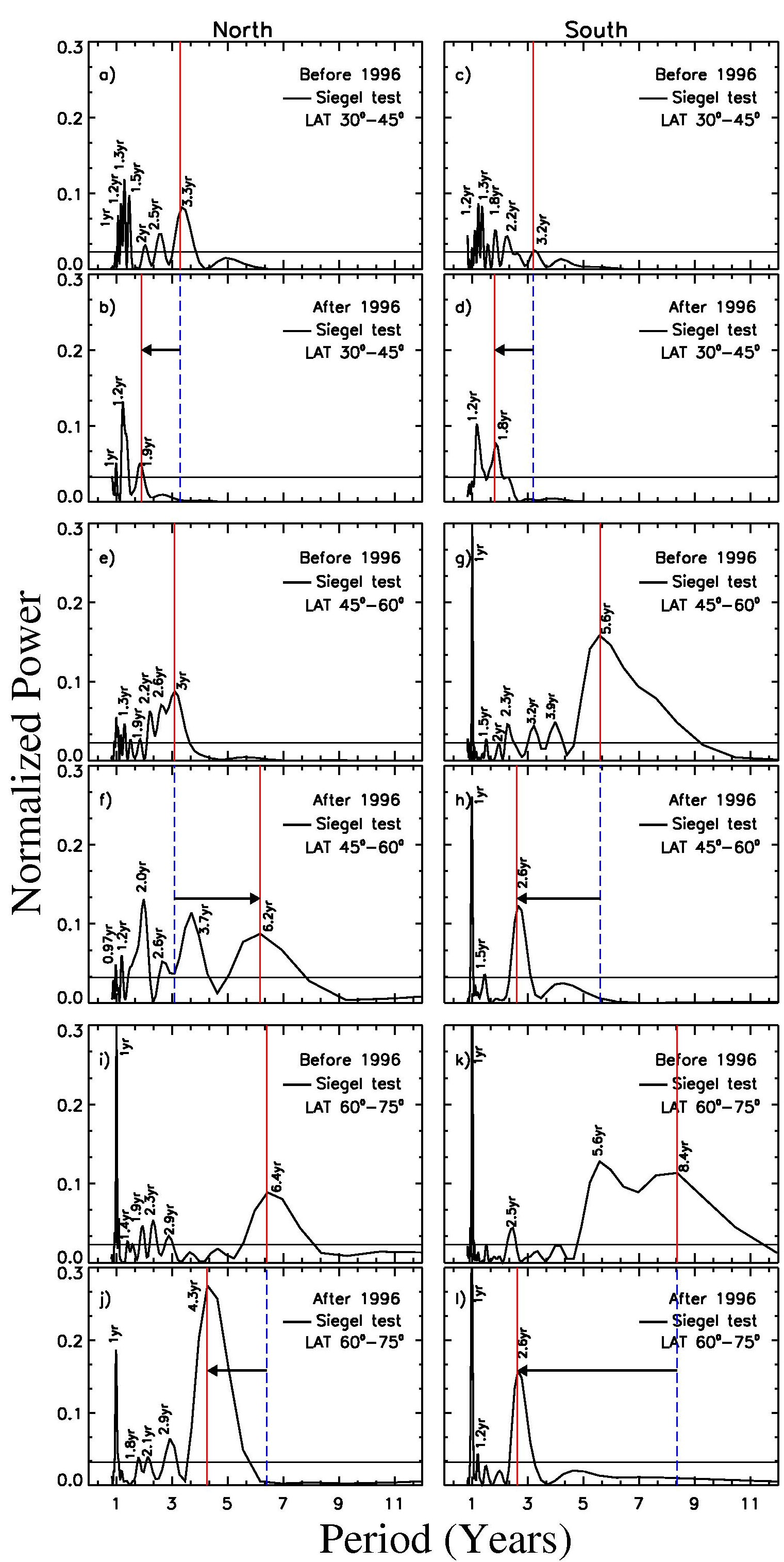
Figure 5: The top four panels - a, b, c, d, the mid - e, f, g, h, and the bottom four panels - i, j, k, l respectively represent the normalized Fourier periodograms for the photospheric fields in the latitude ranges, 30^∘$-$45^∘, 45^∘$-$60^∘, and 60^∘$-$75^∘. The four panels (the top, mid and bottom) in the figure correspond to the Fourier spectral power for magnetic fields in the north before 1996, for magnetic fields in the north after 1996, for magnetic fields in the south before 1996, and for magnetic field in the south after 1996. The solid red vertical line, the dotted blue vertical line and the black arrow in each panel are used to show the shift in periodicity and the spectral power of the fields before and after 1996 both in the northern and southern hemisphere. The solid horizontal lines depict significance levels as determined by Siegel test.

We have generated a butterfly diagram from the NSO/Kitt-Peak synoptic maps by using longitudinally averaged photospheric fields derived from the synoptic maps described in section Decline in mid to high latitude solar fields. Figure 6 shows a butterfly diagram for solar cycles 21, 22 and 23 covering the period from 19 February 1975 to 09 November 2009 (1975.14 $-$ 2009.86). The leading and following polarity fluxes in panel - a of Fig. 6 are shown in red and green respectively for the northern hemisphere in cycle 21, with the derived flux values indicated in a colour coded bar at the top of the figure. It must be noted that leading and following polarity fluxes will be reversed in the southern hemisphere and will again flip from cycle to cycle and hemisphere to hemisphere.

In order to obtain better contrast, the fluxes in Fig. 6a have been limited to the range $\pm 30$G. The poleward motion of the trailing polarity fluxes, above the latitudes ${\pm}$45^∘, known as polar surges are episodic in nature (Wang, Nash, and Sheeley, 1989) and can be clearly seen as tongues of red and green bands in the upper panel of Fig. 6 labeled - a. For a better view of the polar surges, the middle and lower panels of Fig. 6 show variations of intensity as a function of time in each 1^∘ strip of latitude in the latitude range 45^∘$-$60^∘ for the northern hemisphere (middle panel - b) and southern hemisphere (lower panel - c). The solar field for each degree of latitude has been shown after smoothing over three Carrington rotations. An example of a surge in the north and south has been highlighted in red.

Knaack, Stenflo, and Berdyugina (2005) reported a periodicity of 1.3 yr in the photospheric fields that has been correlated with these polar surge motions. We see an approximate periodicity of 1 yr in the polar surge flows in the lower two panels of Fig. 6. This agrees with the strong 1 yr periodicity seen in Fig. 4 and 5. Further, a variation in the strength and occurrence rate of surges prior to and after 1996 can be seen from a careful inspection of Fig. 6a, b and c. In the latitude bin ${\pm}$45^∘ $-$ ${\pm}$60^∘, we find that the frequency of these surges are comparatively more during the years 1996$-$2009 while it is less during the years 1986$-$1995.

Fourier periodicity - Low and high frequency periods

The harmonic analysis yielded Fourier components with periods ranging from 54 d to 12 yr corresponding to a frequency range of 2.6 nHz to 214 nHz. The significant periodic components, as determined by Siegel test, were grouped into low frequency periods in the frequency range, 38.5 nHz (300 d) to 2.6 nHz (12 yr) and high frequency periods in the frequency range, 214 nHz (54 d) to 38.5 nHz (300 d). These periods have been listed in Table 1 (long periods) and Table 2 (short periods) respectively. Many of these periodicities have already been reported by other workers and a few new periodicities have also been seen in our analysis. These new periodicities have been listed in bold face in Tables 1 and 2 and boxed in blue in Figures 4 and 7.

The low frequency periods

In the low frequency range, 38.5 nHz (300 d) to 2.6 nHz (12 yr), we restrict our analysis to periodicities in the range, 305 d to 5.6 yr. Periodicities greater than 5.6 yr are not taken into account because of their inaccurate determination as a consequence of division of time series. The periodicities are listed in Table 1 where the upper half lists periodicities for high-latitude fields in the north and south grouped before and after 1996 while the lower half lists periodicities for low-latitude fields in a similar fashion.

For photospheric fields in the high-latitude range we find periodicities of 305 d (0.84 yr), 325 d (0.89 yr), 339 d (0.92yr), 341 d (0.93 yr), 1 yr, 1.2 yr, 1.4 yr, 1.5 yr, 2 yr, 2.4 yr, 2.6 yr, and 4 yr while for photospheric fields in the low-latitude range we find periods of 312 d (0.86 yr), 318 d (0.87 yr), 321 d (0.88 yr), 327 d (0.9 yr), and 343 d (0.94 yr), 1 yr, 1.27 yr, 1.3 yr, 1.44 yr, 1.5 yr, 1.8 yr, 2.6 yr, 3.5 yr, and 4 yr. All of these quasi-periodicities in various types of solar activity have been reported earlier by other researchers (Howe et al., 2000; Krivova and Solanki, 2002; Knaack, Stenflo, and Berdyugina, 2005; Mendoza, Velasco, and Valdés-Galicia, 2006; Chowdhury, Khan, and Ray, 2009). Knaack, Stenflo, and Berdyugina (2005) had discussed a north-south asymmetry in quasi-periodic variations in unsigned photospheric flux with periods of 1.3yr, 1.5 yr, and 2.6 yr.

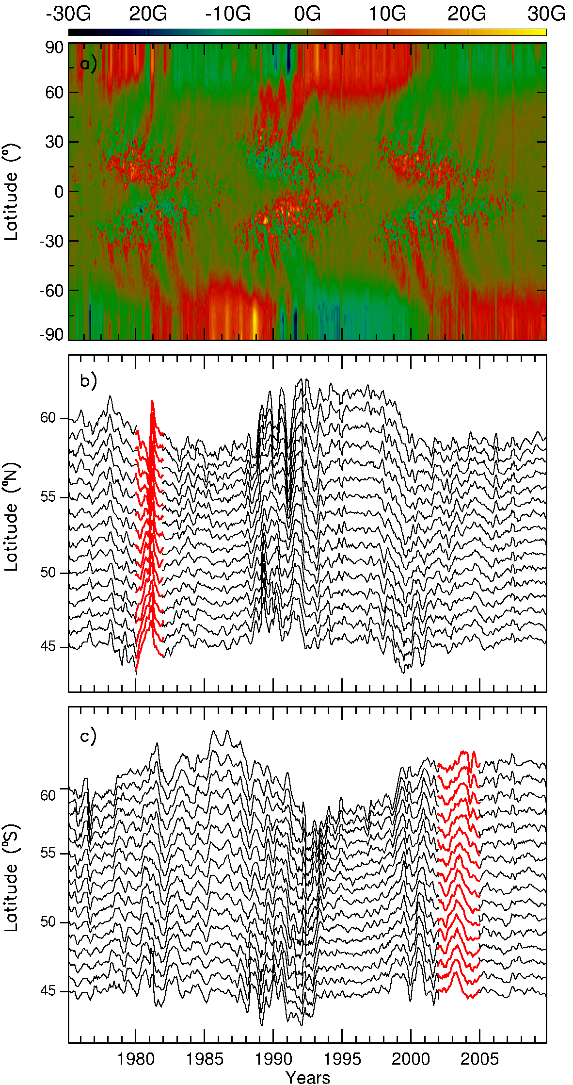
Figure 6: The top panel labeled - a shows a magnetic butterfly diagram generated using NSO/Kitt-Peak magnetograms and depicts the net photospheric magnetic flux distribution on the sun for solar cycles 21, 22 and 23. For better contrast the magnetic flux has been limited to 30 Gauss. The positive and negative polarities are shown in red and green respectively. Polar surges or lateral motions of magnetic flux moving polewards above latitudes of $\pm$45^∘ are seen as tongues of red and green bands. The lower two panels labeled - b and c show the variation of magnetic field, after smoothing over three Carrington rotations, for each degree of latitude in the range 45^∘ to 60^∘. An example of a surge is highlighted in red in the bottom two panels representing the northern and southern hemisphere respectively.

In addition to these known periodicities, we have found some new periodicities in the high-latitude fields with periods 2.3 yr, 2.9 yr, 3.1 yr, and 5.6 yr and in low-latitude fields with periods 1.1 yr, 1.9 yr, 2.5 yr, and 3.1yr. These new periodicities have been shown in boldface in Tables 1 and 2. Though the periodicity of 1 yr has already been reported, we find this periodicity to be the prominent periodicity observed in both north and south high-latitude fields before and after 1996. The Fourier power in the 1 yr period is comparatively more both in the north and south prior to 1996 than after 1996. On the other hand, though the 1 yr period is present in the low-latitude fields both in the north and south, it is only present after 1996. Besides these, periods 1.2$-$1.6 yr is common to both the north and south low-latitude fields and have significant power.

	North High-latitude Field				South High-latitude Field
	Before 96		After 96		Before 96		After 96
	Period(yr)	Power	Period(yr)	Power	Period(yr)	Power	Period(yr)	Power
	$\bf{2.9}$	$\bf{0.04}$	4.0	0.19	$\bf{5.6}$	$\bf{0.13}$	2.6	0.15
	$\bf{2.3}$	$\bf{0.04}$	2.0	0.08	4.0	0.05	1.5	0.04
	2.0	0.02	1.2	0.04	$\bf{3.1}$	$\bf{0.04}$	1.0	0.28
	1.4	0.02	1.0	0.16	2.4	0.05	—	—
	1.0	0.25	0.89	0.04	2.0	0.02	—	—
	0.93	0.06	—	—	1.5	0.04	—	—
	—	—	—	—	1.0	0.02	—	—
	—	—	—	—	0.92	0.03	—	—
	—	—	—	—	0.89	0.02	—	—
	—	—	—	—	0.84	0.04	—	—
	—	—	—	—	—	—	—	—
	North Low-latitude Field				South Low-latitude Field
	Before 96		After 96		Before 96		After 96
	Period(yr)	Power	Period(yr)	Power	Period(yr)	Power	Period(yr)	Power
	3.5	0.09	1.5	0.05	4.0	0.03	$\bf{1.9}$	$\bf{0.25}$
	$\bf{2.5}$	$\bf{0.10}$	1.0	0.04	$\bf{3.1}$	$\bf{0.09}$	$\bf{1.1}$	$\bf{0.04}$
	1.5	0.11	0.86	0.07	2.6	0.1	0.90	0.05
	1.3	0.04	—	—	1.8	0.05	—	—
	0.88	0.04	—	—	1.5	0.05	—	—
	—	—	—	—	1.44	0.04	—	—
	—	—	—	—	1.27	0.04	—	—
	—	—	—	—	0.94	0.04	—	—
	—	—	—	—	0.87	0.06	—	—

Table 1: The Fourier periods in the frequency range, 38.5 nHz to 2.6 nHz (Low frequency zone), are listed with their Fourier power respectively in the upper and lower half of the table for high-latitude fields and low-latitude fields in both the north and south prior to 1996 and after 1996.

	North High-latitude Field				South High-latitude Field
	Before 96		After 96		Before 96		After 96
	Period(day)	Power	Period(day)	Power	Period(day)	Power	Period(day)	Power
	$\bf{294}$	$\bf{0.02}$	$\bf{253}$	$\bf{0.04}$	288	0.037	184	0.07
	278	0.06	183	0.061	184	0.06	—	—
	263	0.04	—	—	—	—	—	—
	240	0.02	—	—	—	—	—	—
	183	0.04	—	—	—	—	—	—
	157	0.04	—	—	—	—	—	—
	North Low-latitude Field				South Low-latitude Field
	Before 96		After 96		Before 96		After 96
	Period(day)	Power	Period(day)	Power	Period(day)	Power	Period(day)	Power
	288	0.02	$\bf{257}$	$\bf{0.04}$	283	0.04	—	—
	278	0.03	181	0.08	248	0.02	—	—
	261	0.03	172	0.11	228	0.03	—	—
	—	—	147	0.04	157	0.03	—	—
	—	—	—	—	151	0.03	—	—
	—	—	—	—	145	0.03	—	—
	—	—	—	—	—	—	—	—
	—	—	—	—	—	—	—	—

Table 2: The Fourier periods with their Fourier spectral power in the frequency range, 214 nHz to 38.5 nHz (High frequency zone) are listed respectively in the upper and lower half of the table for high-latitude fields and low-latitude fields both in the north and south prior to 1996 and after 1996.

Among these periodicities, the most discussed and reported periodicity is the 1.3 yr periodicity (Krivova and Solanki, 2002; Knaack, Stenflo, and Berdyugina, 2004, 2005) which has been linked to polar surges that can be seen most clearly in the latitude band 45^∘ to 60^∘ (Wang, Nash, and Sheeley, 1989; Knaack, Stenflo, and Berdyugina, 2005) in magnetic butterfly diagrams as depicted in Fig. 6. Also, the 1.3 yr periodicity has been linked to the variation of the rotation rate near the base of the convection zone (Howe et al., 2000).

The high frequency periods

In the high frequency range we have frequencies ranging from 214 nHz (54 d) to 38.5 nHz (300 d). These periodicities for both the high-latitude and low-latitude fields are listed in the Table 2. The upper half of the Table 2 lists periodicities for the high-latitude fields with periods ranging between 157 d to 294 d. Few of these periodicities with their Fourier spectral power are shown in the top four panels - a, b, c, d in Fig 7. Similarly, the lower half of the Table 2 lists significant periodicities for the low-latitude fields with periods ranging in between 134 d to 288 d. The bottom four panels - e, f, g, h in Fig 7 show a few of these periodicities with their spectral power. As stated earlier the significant periodic components were determined using the Siegel test statistics and are those periodic components having power levels above the black horizontal line drawn in each panel of Fig. 7.

The known periodicities in the high-latitude zone include those with periods 157 d, 183 d, 184 d, 240 d, 263 d, 278 d, and 288 d and the new periodicities ${\it{viz.}}$ with period 253 d and 294 d, not reported in the literature earlier, are shown in boldface in the upper part of the Table 2.

The Rieger periodicity of 157 d is a well known fundamental periodicity that we find only in the high-latitude fields in the northern hemisphere prior to 1996. In addition, the periodicity of 182$-$184 d is seen to be always present and the Fourier power corresponding to this periodicity does not vary much in both the north and south fields at high latitudes both before and after 1996. These high-frequency periods, in the high-latitude fields, don’t show much variation in their normalized Fourier power and we do not see any north-south asymmetry in these high-latitude fields.

On the other hand, in the low-latitude zone, shown in the lower part of the Table 2, we report periodicities of 145 d, 147 d, 151 d, 157 d, 172 d, 228 d, 248 d, 261 d, 278 d, 283 d and 288 d, which have already been reported in earlier work (Oliver, Ballester, and Baudin, 1998; Krivova and Solanki, 2002; Knaack, Stenflo, and Berdyugina, 2005; Chowdhury, Khan, and Ray, 2009). The new periodicity from our analysis was 257 d and is shown in boldface in the lower half of the Table 2. The Rieger periodicity of 157 d is only seen in the south low-latitude field before 1996. Also, the semi-annual variation of period 181 d is observed only in north low-latitude fields.

Discussion and Conclusion

Our wavelet analysis shows a transition occurring around 1996 in the distribution of power and periodicities of photospheric fields. When the data were partitioned into periods prior to and after 1996 a hemispheric asymmetry is seen in the derived Fourier periodicities of solar magnetic activity above latitudes of $\pm$45^∘. A more detailed analysis shows that this asymmetry is confined to the latitude band 45^∘$-$60^∘ in both hemispheres. This latitude band is primarily dominated by strong, episodic poleward surges or tongues of magnetic flux in both hemispheres which, as stated earlier, are a direct surface manifestation of the meridional flow and the internal solar dynamo. In the 60^∘$-$75^∘ latitude band we find an asymmetry in the distribution of spectral power in the longer periods since the photospheric surface fields have saturated in this band. This observed and localized asymmetry, confined to the 45^∘$-$60^∘ latitude zone in both hemispheres, when coupled with the fact that both solar fields and the micro-turbulence levels in the inner-heliosphere have been decreasing since early to mid nineties suggests that active changes occurred around this time in the solar dynamo that governs the underlying basic processes in the sun. These changes in turn probably initiated the build-up to one of the deepest solar minima, at the end of the cycle 23, experienced in the past 100 years.

Figure 7: The top four panels - a , b, c, d and the bottom four panels - e, f, g, h respectively represent the normalized Fourier periodograms for high-latitude fields and low-latitude fields for the high frequency periods in the frequency range 214 nHz to 38.5 nHz . The respective four panels in the top and the bottom show the normalized Fourier power distribution with periodicity for photospheric fields in the north before 1996, in the north after 1996, in the south before 1996 and in the south after 1996. The new periodicities in our analysis have been boxed in blue.

The magnetic time series in both the solar hemispheres exhibit a multitude of periodicities with significant variation in the spectral power of midterm (1$-$2 year) periodicities before and after 1996. These prominent periods in the lower solar latitudes, below ${\pm}$45^∘, are thought to originate as the result of stochastic processes caused by the periodic emergence of surface magnetic flux (Wang and Sheeley, 2003) as the solar cycle progresses. As stated earlier, Howe et al. (2000) have reported a 1.3 year periodicity at the base of the solar convection zone, which has also been detected in sunspot areas and sunspot number time series studied using wavelet transforms (Krivova and Solanki, 2002; Chowdhury and Dwivedi, 2011). These findings have led to the conclusion that the mid-term fluctuations in the solar fields are surface manifestations of changes in the magnetic fluxes generated deep inside the Sun.

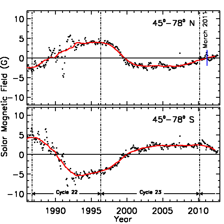
Figure 8: Shows the solar magnetic field in the northern (top) and southern (bottom) hemispheres in the latitude range 45^∘ to 78^∘ for solar cycles 22 and 23. It is clear that the north solar field has reversed while the south solar field is still to do so. The time of reversal of the north solar field is indicated by a small blue arrow.

Polar surges above latitudes ${\pm}$45^∘ show significant variations in their occurrence rates and strength in each cycle and will therefore show up as a variation in spectral power and periods. A comparison of polar surges in the last three solar cycles, viz. 21, 22, and 23, reveals that they are comparatively more in strength after around solar maximum.

Though we have restricted our analysis to data from cycles 21, 22 and 23 in the period from $\sim$1975 $-$ 2010, an examination of data beyond 2010 shows an asymmetry in the solar field reversal at high-latitudes. Figure 8 shows the reversal of the northern high latitude field in cycle 24 in March 2011. However, the southern hemisphere is yet to undergo a reversal. The filled black dots in Fig. 8 are the actual measurements while the red solid line is a smoothed curve. The reversal of the solar polar field occurs at times when the red curve passes through zero and is indicated for cycle 24 by a small blue line in the northern hemisphere. While it is known from earlier cycles that the two hemispheres do not reverse polarities at the same time, the time lag between the reversal of the northern hemisphere and southern hemisphere has, to the best of our knowledge, never been as large.

In addition, Dikpati et al. (2010) and Dikpati (2011), using the theory of meridional circulation, have reported an asymmetry in the latitudinal extent of the Sun’s meridional flow belt in the cycle 22 and 23 wherein surface meridional flows in cycle 22 extend to latitudes of ${\pm}$60^∘ while in cycle 23, it went all the way to the poles. Thus, the meridional flow in cycle 23, took a longer time thereby causing a slower return flow which led in turn to the extended solar minimum in cycle 23. Recent work, using helioseismic data from the Birmingham Solar Oscillation Network (BiSON), an instrument that is very sensitive in probing the solar interior close to the solar surface, has shown that the behavior of solar oscillation frequencies in the sub-surface magnetic layers during the descending phase of cycle 23 was significantly different from that during cycle 22 (Basu et al., 2012). These authors went on to state that the peculiar solar minimum, at the end of the cycle 23, could have been predicted long before it happened. The present work, showing a north-south asymmetry around mid 1990’s in the quasi-periodic variations of photospheric fields at high-latitudes shows that changes were initiated at this time in the basic underlying solar dynamo processes like the meridional flow rates and the magnetic flux emergence that eventually led to the prolonged and deep minimum that we have just witnessed.

The current understanding of the solar dynamo is that it operates through the Babcock-Leighton mechanism to produce poloidal fields through the decay of tilted bipolar sunspots (Choudhuri, Chatterjee, and Jiang, 2007; Jiang, Chatterjee, and Choudhuri, 2007). The strength of the polar field, at each solar maximum then depends upon the tilt angle in bipolar sunspots which, in turn, is determined by the action of the Coriolis force acting on magnetic flux tubes that reach the surface by rising through the turbulent convection zone (D’Silva and Choudhuri, 1993). This process causes a large scatter in the average tilt-angle causing the polar field to be randomly weaker or stronger than in the previous cycle (Longcope and Choudhuri, 2002). We have observed a decline in fields above 45^∘ for the past $\sim$15 years implying weak polar fields being generated in two successive solar cycles viz. cycles 22 and 23. A continuation of this declining trend beyond 22 years would imply a third successive weak polar field imparted by the Babcock-Leighton mechanism. This is probably unlikely as the polar field is imparted by a random process and if it happens it would have serious implications on our present understanding of the solar dynamo. Also, two of the eight strongest geomagnetic storms in the last 150 years have occurred during solar cycles 13 and 14 which were both relatively weak cycles. Therefore, continued observations and measurements of solar magnetic fields are extremely important.

References

- Ananthakrishnan, Balasubramanian, and Janardhan (1995) Ananthakrishnan, S., Balasubramanian, V., Janardhan, P.: 1995, Latitudinal Variation of Solar Wind Velocity. Space Sci. Rev. 72, 229 – 232. doi:10.1007/BF00768784.
- Ananthakrishnan, Coles, and Kaufman (1980) Ananthakrishnan, S., Coles, W.A., Kaufman, J.J.: 1980, Microturbulence in solar wind streams. J. Geophys. Res. 85, 6025 – 6030. doi:10.1029/JA085iA11p06025.
- Bai (1987) Bai, T.: 1987, Periodicities of the flare occurrence rate in solar cycle 19. Astrophys. J. Lett. 318, L85 – L91. doi:10.1086/184943.
- Bai (2003) Bai, T.: 2003, Periodicities in Solar Flare Occurrence: Analysis of Cycles 19-23. Astrophys. J. 591, 406 – 415. doi:10.1086/375295.
- Basu et al. (2012) Basu, S., Broomhall, A.-M., Chaplin, W.J., Elsworth, Y.: 2012, Thinning of the Sun’s magnetic layer: the peculiar solar minimum could have been predicted. ArXiv e-prints.
- Choudhuri, Chatterjee, and Jiang (2007) Choudhuri, A.R., Chatterjee, P., Jiang, J.: 2007, Predicting Solar Cycle 24 With a Solar Dynamo Model. Physical Review Letters 98(13), 131103 – +. doi:10.1103/PhysRevLett.98.131103.
- Chowdhury and Dwivedi (2011) Chowdhury, P., Dwivedi, B.N.: 2011, Periodicities of Sunspot Number and Coronal Index Time Series During Solar Cycle 23. Solar Phys. 270, 365 – 383. doi:10.1007/s11207-011-9738-1.
- Chowdhury and Ray (2006) Chowdhury, P., Ray, P.C.: 2006, Periodicities of solar electron flare occurrence: analysis of cycles 21-23. Mon. Not. Roy. Astron. Soc. 373, 1577 – 1589. doi:10.1111/j.1365-2966.2006.11120.x.
- Chowdhury, Khan, and Ray (2009) Chowdhury, P., Khan, M., Ray, P.C.: 2009, Intermediate-term periodicities in sunspot areas during solar cycles 22 and 23. Mon. Not. Roy. Astron. Soc. 392, 1159 – 1180. doi:10.1111/j.1365-2966.2008.14117.x.
- Chowdhury, Khan, and Ray (2010) Chowdhury, P., Khan, M., Ray, P.C.: 2010, Short-Term Periodicities in Sunspot Activities During the Descending Phase of Solar Cycle 23. Solar Phys. 261, 173 – 191. doi:10.1007/s11207-009-9478-7.
- Dikpati (2011) Dikpati, M.: 2011, Comparison of the Past Two Solar Minima from the Perspective of the Interior Dynamics and Dynamo of the Sun. Space Sci. Rev., 143. doi:10.1007/s11214-011-9790-z.
- Dikpati et al. (2010) Dikpati, M., Gilman, P.A., de Toma, G., Ulrich, R.K.: 2010, Impact of changes in the Sun’s conveyor-belt on recent solar cycles. Geophys. Res. Lett. 37, 14107. doi:10.1029/2010GL044143.
- Droege et al. (1990) Droege, W., Gibbs, K., Grunsfeld, J.M., Meyer, P., Newport, B.J., Evenson, P., Moses, D.: 1990, A 153 day periodicity in the occurrence of solar flares producing energetic interplanetary electrons. Astrophys. J. Supplement. 73, 279 – 283. doi:10.1086/191463.
- D’Silva and Choudhuri (1993) D’Silva, S., Choudhuri, A.R.: 1993, A theoretical model for tilts of bipolar magnetic regions. Astron. Astrophys. 272, 621.
- Fisher (1929) Fisher, R.A.: 1929, Tests of Significance in Harmonic Analysis. Royal Society of London Proceedings Series A 125, 54 – 59.
- Forrest et al. (1980) Forrest, D.J., Chupp, E.L., Ryan, J.M., Cherry, M.L., Gleske, I.U., Reppin, C., Pinkau, K., Rieger, E., Kanbach, G., Kinzer, R.L.: 1980, The gamma ray spectrometer for the Solar Maximum Mission. Solar Phys. 65, 15 – 23. doi:10.1007/BF00151381.
- Hathaway and Rightmire (2010) Hathaway, D.H., Rightmire, L.: 2010, Variations in the Sun’s Meridional Flow over a Solar Cycle. Science 327, 1350. doi:10.1126/science.1181990.
- Howard (1974) Howard, R.: 1974, Studies of solar magnetic fields. II - The magnetic fluxes. Solar Phys. 38, 59 – 67. doi:10.1007/BF00161823.
- Howe et al. (2000) Howe, R., Christensen-Dalsgaard, J., Hill, F., Komm, R.W., Larsen, R.M., Schou, J., Thompson, M.J., Toomre, J.: 2000, Dynamic Variations at the Base of the Solar Convection Zone. Science 287, 2456 – 2460. doi:10.1126/science.287.5462.2456.
- Janardhan, Bisoi, and Gosain (2010) Janardhan, P., Bisoi, S.K., Gosain, S.: 2010, Solar Polar Fields During Cycles 21 - 23: Correlation with Meridional Flows. Solar Phys. 267, 267 – 277. doi:10.1007/s11207-010-9653-x.
- Janardhan et al. (2011) Janardhan, P., Bisoi, S.K., Ananthakrishnan, S., Tokumaru, M., Fujiki, K.: 2011, The prelude to the deep minimum between solar cycles 23 and 24: Interplanetary scintillation signatures in the inner heliosphere. Geophys. Res. Lett. 382, 20108. doi:10.1029/2011GL049227.
- Jian, Russell, and Luhmann (2011) Jian, L.K., Russell, C.T., Luhmann, J.G.: 2011, Comparing Solar Minimum 23/24 with Historical Solar Wind Records at 1 AU. Solar Phys., 69 – +. doi:10.1007/s11207-011-9737-2.
- Jiang, Chatterjee, and Choudhuri (2007) Jiang, J., Chatterjee, P., Choudhuri, A.R.: 2007, Solar activity forecast with a dynamo model. Mon. Not. Roy. Astron. Soc. 381, 1527 – 1542. doi:10.1111/j.1365-2966.2007.12267.x.
- Jiang et al. (2011) Jiang, J., Cameron, R.H., Schmitt, D., Schussler, M.: 2011, Can Surface Flux Transport Account for the Weak Polar Field in Cycle 23? Space Sci. Rev., 136. doi:10.1007/s11214-011-9783-y.
- Kile and Cliver (1991) Kile, J.N., Cliver, E.W.: 1991, A search for the 154 day periodicity in the occurrence rate of solar flares using Ottawa 2.8 GHz burst data, 1955-1990. Astrophys. J. 370, 442 – 448. doi:10.1086/169831.
- Kiliç (2008) Kiliç, H.: 2008, Midrange periodicities in sunspot numbers and flare index during solar cycle 23. Astron. Astrophys. 481, 235 – 238. doi:10.1051/0004-6361:20078455.
- Kirk et al. (2009) Kirk, M.S., Pesnell, W.D., Young, C.A., Hess Webber, S.A.: 2009, Automated detection of EUV Polar Coronal Holes during Solar Cycle 23. Solar Phys. 257, 99 – 112. doi:10.1007/s11207-009-9369-y.