Mean-Variance Asset-Liability Management with State-Dependent Risk Aversion

Abstract

In this paper, we consider the asset-liability management under the mean-variance criterion. The financial market consists of a risk-free bond and a stock whose price process is modeled by a geometric Brownian motion. The liability of the investor is uncontrollable and is modeled by another geometric Brownian motion. We consider a specific state-dependent risk aversion which depends on a power function of the liability. By solving a flow of FBSDEs with bivariate state process, we obtain the equilibrium strategy among all the open-loop controls for this time-inconsistent control problem. It shows that the equilibrium strategy is a feedback control of the liability.

Keywords: Asset-liability management; Mean-variance; Equilibrium strategy; Time-inconsistent control problem; FBSDEs

1 Introduction

In the pioneer work Markowitz (1952), the author considered the portfolio selection under the well-known mean-variance criterion and derived the analytical expression of the mean-variance efficient frontier in the single-period model. This seminal work has become the foundation of modern portfolio theory and has stimulated numerous extensions.

On the one hand, some researchers focus on studying the dynamic mean-variance portfolio selection problem. Samuelson (1969) considered a discrete-time multi-period model. More recently, by embedding the original problem into a stochastic linear-quadratic (LQ) control problem, Li and Ng (2000) and Zhou and Li (2000) extended Markowitz’s work to a multi-period model and a continuous-time model, respectively. On the other hand, there are some works that consider a generalized financial market. An important and popular subject is the asset and liability management problem, which studies the selection of portfolio while taking into account the liabilities of investors. More specifically, in the asset and liability management, the surplus, i.e. the difference between asset value and liability value, is considered.

Since it was proposed by Sharpe and Tint (1990) which considered a single-period model, there is an increasing number of interests in the asset-liability management under the mean-variance criteria. Keel and Müller (1995) studied the portfolio choice with liabilities and showed that liabilities affect the efficient frontier. Adopting the embedding technique of Li and Ng (2000), Leippold et al. (2004) derived an analytical optimal policy and efficient frontier for the multi-period asset-liability management problem. The mean-variance asset-liability management in a continuous-time model was investigated by Chiu and Li (2006) in which a stochastic LQ control problem was studied and both the optimal strategy and the mean efficient frontier were obtained. Furthermore, in a regime-switching framework, Chen et al. (2008) and Chen and Yang (2011) studied the mean-variance asset-liability management in the continuous-time model and mule-period model, respectively. It is worth to note that, all of these papers suggested that the liabilities were not controllable, which is the main difference between the Markowitz’s problem and the asset-liability management.

It is well acknowledged that due to the existence of a non-linear function of the expectation in the objective functional, the mean-variance portfolio selection problem in a multi-period framework is time inconsistent in the sense that the Bellman optimality principle does not hold. Intuitively, an optimal strategy obtained for the initial time may not be optimal for any latter time. This is the so-called pre-committed strategy, i.e., the strategy that is only optimal for the initial time. Note that in all the references we mentioned above (among others), only the pre-committed strategies have been considered.

In Strotz (1955), the author proposed another approach to study the time inconsistent problem, i.e., study the problem within a game theoretic framework by using Nash equilibrium points. Recently, there is an increasing amount of attention in the time inconsistent control problem due to the practical applications in the economics and finance. In Ekeland and Lazrak (2006) and Ekeland and Pirvu (2008) which considered the optimal consumption and investment problem under hyperbolic discounting, the authors provided the precise definition of the equilibrium concept in continuous time for the first time. Following their idea, Björk and Murgoci (2010) studied the time-inconsistent control problem in a general Markov framework, and derived the extended HJB equation together with the verification theorem. Björk et al. (2012) studied the Markowitz’s problem with state-dependent risk aversion by utilizing the extended HJB equation obtained in Björk and Murgoci (2010). They showed that the equilibrium control was dependent on the current state. Considering a regime-switching model and with the assumption that the risk aversion depends on the state of the regime, Wei et al. (2012) investigated the equilibrium strategy for the mean-variance asset-liability management problem by using the extended HJB equation developed by Björk and Murgoci (2010).

In Ekeland and Lazrak (2006), Ekeland and Pirvu (2008) and the papers following their idea, the equilibrium control was defined within the class of feedback controls. Considering the time-inconsistent stochastic LQ control, Hu et al. (2012) defined the equilibrium control within the class of open-loop controls, and derived a general sufficient condition for equilibriums through a flow of forward-backward stochastic differential equations (FBSDEs). However, the general existence of solutions to the flow of FBSDEs is an open problem. With the assumption that the state process was scalar valued and all the coefficients were deterministic, Hu et al. (2012) showed that the flow of FBSDEs could be reduced into several Riccati-like ordinary differential equations and the equilibrium control could be obtained explicitly. Also considering the scalar valued state process, Hu et al. (2012) dealt with the Markowitz’s problem with state-dependent risk aversion and stochastic coefficients. Due to the difference between the definitions of equilibrium controls, their results were rather different from those obtained in Björk and Murgoci (2010) and Björk et al. (2012).

Following the idea of Hu et al. (2012), we consider the time-inconsistent mean-variance asset-liability management. Since the state process of our problem is bivariate, the solution to the flow of FBSDEs in Hu et al. (2012) can not be directly adopted. We show that the flow of FBSDEs of our problem can be solved explicitly and the (close-form) equilibrium strategy can be obtained. There are some differences between this paper and Wei et al. (2012) which also studied the time-inconsistent mean-variance asset-liability management. First, the definitions of equilibrium controls are different. They are inherited from the differences between Hu et al. (2012) and Ekeland and Pirvu (2008). Second, the risk aversion considered in this paper depends on the liability process (see Remark 2.2), while the risk aversion in Wei et al. (2012) only depends on the state of regime and it becomes constant when there is only one regime. Since the risk aversion is independent of the surplus process, the equilibrium strategy in this paper is a feedback control of the liability process which is similar to Wei et al. (2012). Although we use different definitions of the equilibrium strategy from Wei et al. (2012), in a special case we get the same result with Wei et al. (2012) (see Remark 3.2).

The remainder of this paper is organized as follows. Section 2 introduces the model, the definition of the equilibrium strategy and the flow of FBSDEs of our problem. In section 3 we derive the solution to the flow of FBSDEs and the equilibrium strategy. Section 4 establishes the equilibrium value function. Some numerical examples are illustrated in section 5.

2 Preliminaries

2.1 The model

Let $\left(\Omega,\mathcal{F},\hbox{\sf P}\right)$ be a fixed complete probability space on which two independent standard Brownian motions $W_{1}(t)$ and $W_{2}(t)$ are defined. Let $T>0$ be the fixed and finite time horizon and denote by $\left\{\mathcal{F}_{t}\right\}_{t\in[0,T]}$ the augmented filtration generated by $(W_{1}(t),W_{2}(t))$.

We introduce the following notation with $n$ being a generic integer:

$$L_{\mathcal{G}}^{2}(\Omega;\mathbb{R}^{n}): \quad\text{the set of random variables }\xi:(\Omega,\mathcal{G})\rightarrow(\mathbb{R}^{n},\mathcal{B}(\mathbb{R}^{n}))\text{ with \hbox{\sf E}$\left[\left|\xi\right|^{2}\right]$<+$\infty$.}$$

$$L_{\mathcal{G}}^{2}(t,T;\mathbb{R}^{n}): \quad\text{the set of }\{\mathcal{G}\}_{s\in[t,T]}\text{-adapted processes }\{f(s)\}_{s\in[t,T]}$$

$$\quad\text{ with }\hbox{\sf E}\left[\int_{t}^{T}\left|f(s)\right|^{2}\mathrm{d}s\right]<\infty.$$

$$L_{\mathcal{G}}^{2}(\Omega;C(t,T,\mathbb{R}^{n})): \quad\text{the set of continuous }\{\mathcal{G}\}_{s\in[t,T]}\text{-adapted processes }\{f(s)\}_{s\in[t,T]}$$

$$\quad\text{ with }\hbox{\sf E}\left[\sup_{s\in[t,T]}\left|f(s)\right|^{2}\right]<\infty.$$

In what follows, unless otherwise specified, we adopt bold-face letters to denote matrices and vectors, and the transpose of a matrix or vector $\mathbf{M}$ is denoted by $\mathbf{M}^{\prime}$. Also, we denote by $M_{ij}$ (or $M_{i}$) the $(i,j)$-element (or the $i$-th element) of the matrix $\mathbf{M}$ (or the vector $\mathbf{M}$).

We consider a financial market consisting of one bond and one stock within the time horizon $[0,T]$. The price of the risk-free bond $B(t)$ satisfies

$$\mathrm{d}B(t)=r(t)B(t)\mathrm{d}t,\quad B(0)=1,\quad 0\leq t\leq T.$$

The price of the stock $P(t)$ is given by

$$\mathrm{d}P(t)=P(t)\left[\mu(t)\mathrm{d}t+\sigma(t)\mathrm{d}W_{1}(t)\right],\quad 0\leq t\leq T,$$

where $P(0)=p_{0}>0.$

Denote by $L(t)$ the liability of the investor. We assume that the liability and the stock price are correlated and the dynamics of liability is given by

$$\mathrm{d}L(t)=L(t)\left[\alpha(t)\mathrm{d}t+\rho(t)\beta(t)\mathrm{d}W_{1}(t)+\sqrt{1-\rho^{2}(t)}\beta(t)\mathrm{d}W_{2}(t)\right],\quad 0\leq t\leq T,$$

where $L(0)=l_{0}>0$ and $\rho(t)\in[0,1]$ for all $t\in[0,T]$.

Let $u(t)$ be the dollar amount invested in the stock at time $t$. Then the asset in the stock market $Z(t)$ evolves as

$$\mathrm{d}Z(t)=\left[r(t)Z(t)+(\mu(t)-r(t))u(t)\right]\mathrm{d}t+\sigma(t)u(t)\mathrm{d}W_{1}(t),\quad 0\leq t\leq T,$$

where $Z(0)=z_{0}.$ The surplus process for the asset-liability management is given by $S(t):=Z(t)-L(t).$ Then the dynamics of $S(t)$ is

$$\mathrm{d}S(t) = \left[r(t)S(t)+\eta(t)L(t)+\theta(t)u(t)\right]\mathrm{d}t+\left[\sigma(t)u(t)-\rho(t)\beta(t)L(t)\right]\mathrm{d}W_{1}(t)$$

$$-\sqrt{1-\rho^{2}(t)}\beta(t)L(t)\mathrm{d}W_{2}(t),\qquad 0\leq t\leq T,$$

where $\eta(t)=r(t)-\alpha(t)$, $\theta(t)=\mu(t)-r(t)$ and $S(0)=z_{0}-l_{0}:=s_{0}$.

Let $\mathbf{X}(t)=(S(t),L(t))^{\prime}$ be the bivariate state process and $\mathbf{X}(0)=\mathbf{x}_{0}:=(s_{0},l_{0})^{\prime}$. Thus we have

$$\mathrm{d}\mathbf{X}(t)=\left[\mathbf{A}(t)\mathbf{X}(t)+\mathbf{B}^{\prime}(t)u(t)\right]\mathrm{d}t+\left[\mathbf{C}_{1}(t)\mathbf{X}(t)+\mathbf{D}(t)u(t)\right]\mathrm{d}W_{1}(t)+\mathbf{C}_{2}(t)\mathbf{X}(t)\mathrm{d}W_{2}(t),$$ (2.1)

where

$$\mathbf{A}(t)=\begin{pmatrix}r(t)&\eta(t)\\ 0&\alpha(t)\end{pmatrix},\quad\mathbf{B}(t)=(\theta(t),0),\quad\mathbf{C}_{1}(t)=\begin{pmatrix}0&-\rho(t)\beta(t)\\ 0&\rho(t)\beta(t)\end{pmatrix},\quad\mathbf{C}_{2}(t)=\begin{pmatrix}0&-\sqrt{1-\rho^{2}(t)}\beta(t)\\ 0&\sqrt{1-\rho^{2}(t)}\beta(t)\end{pmatrix},$$

and $\mathbf{D}(t)=(\sigma(t),0)^{\prime}$. We assume that $\mathbf{A}$ $\mathbf{B},\mathbf{C}_{1},\mathbf{C}_{2}$ and $\mathbf{D}$ are bounded deterministic functions on $[0,T]$ valued in $\mathbb{R}^{2\times 2}$, $\mathbb{R}^{1\times 2},\mathbb{R}^{2\times 2},\mathbb{R}^{2\times 2}$ and $\mathbb{R}^{2\times 1}$, respectively.

Definition 2.1.

A strategy $u$ is said to be admissible if $u\in L_{\mathcal{F}}^{2}(0,T;\mathbb{R})$ such that SDE (2.1) has a unique solution $\mathbf{X}\in L_{\mathcal{F}}^{2}(\Omega;C(0,T,\mathbb{R}^{2}))$.

For the time-inconsistent control problem, we will consider the controlled state process starting from time $t\in[0,T]$ and state $\mathbf{x}_{t}\in L_{\mathcal{F}}^{2}(\Omega,\mathbb{R}^{2})$:

$$\mathrm{d}\mathbf{X}(s)=\left[\mathbf{A}(s)\mathbf{X}(s)+\mathbf{B}^{\prime}(s)u(s)\right]\mathrm{d}s+\left[\mathbf{C}_{1}(s)\mathbf{X}(s)+\mathbf{D}(s)u(s)\right]\mathrm{d}W_{1}(s)+\mathbf{C}_{2}(s)\mathbf{X}(s)\mathrm{d}W_{2}(s),$$ (2.2)

with $\mathbf{X}(t)=\mathbf{x}_{t}.$ Note that for any strategy $u\in L_{\mathcal{F}}^{2}(t,T;\mathbb{R})$, SDE (2.2) admits a unique solution $\mathbf{X}^{t,\mathbf{x}_{t},u}\in L_{\mathcal{F}}^{2}(\Omega;C(t,T,\mathbb{R}^{2}))$.

At any initial state $(t,\mathbf{x}_{t})$, the mean-variance cost functional is given by

$$J(t,\mathbf{x}_{t};u) := \frac{1}{2}\hbox{\sf Var}\,_{t}\left[S(T)\right]-\left[\omega_{1}L^{-\lambda}(t)+\omega_{2}\right]\hbox{\sf E}_{t}\left[S(T)\right]$$ (2.3)

$$= \frac{1}{2}\hbox{\sf E}_{t}\left[S^{2}(T)\right]-\frac{1}{2}\left(\hbox{\sf E}_{t}\left[S(T)\right]\right)^{2}-\left[\omega_{1}L^{-\lambda}(t)+\omega_{2}\right]\hbox{\sf E}_{t}\left[S(T)\right],$$

where $u\in L_{\mathcal{F}}^{2}(t,T;\mathbb{R})$, $(S,L)^{\prime}=\mathbf{X}^{t,\mathbf{x}_{t},u}$, $\omega_{1}$ , $\omega_{2}$ , $\lambda$ are nonnegative constants, and $\hbox{\sf E}_{t}[\cdot]:=\hbox{\sf E}[\cdot\mid\mathcal{F}_{t}]$.

Remark 2.2.

Note that $\frac{1}{\omega_{1}L^{-\lambda}(t)+\omega_{2}}$ is a state-dependent risk aversion of the investor. Taking $\omega_{1}\geq 0$ and $\lambda\geq 0$ implies that the risk aversion increases with increasing liability which is reasonable for a common investor. Noting that, with such a risk aversion, the investor is uniformly risk averse.

2.2 The equilibrium strategy

In this subsection, we introduce the equilibrium strategy to the time-inconsistent control problem. We use the definition of the equilibrium strategy from Hu et al. (2012).

Definition 2.3.

Let $u^{*}\in L_{\mathcal{F}}^{2}(0,T;\mathbb{R})$ be a given strategy and $\mathbf{X}^{*}$ be the state process corresponding to $u^{*}$. The strategy $u^{*}$ is called an equilibrium strategy if for any $t\in[0,T)$ and $v\in L_{\mathcal{F}_{t}}^{2}(\Omega,\mathbb{R})$,

$$\liminf_{\epsilon\rightarrow 0}\frac{J(t,\mathbf{X}^{*}(t);u^{t,\epsilon,v})-J(t,\mathbf{X}^{*}(t);u^{*})}{\epsilon}\geq 0,$$

where

$$u^{t,\epsilon,v}(s):=u^{*}(s)+v\hbox{\bf 1}_{s\in[t,t+\epsilon]},\quad s\in[t,T],$$

for any $t\in[0,T)$ and $\epsilon>0$. The equilibrium value function is defined by

$$V(t,\mathbf{X}^{*}(t)):=J(t,\mathbf{X}^{*}(t);u^{*}).$$ (2.4)

Although we have stated the difference between definitions of equilibrium strategy in Hu et al. (2012) and Ekeland and Lazrak (2006) in previous section, they have similar intuition. We refer the reader to these papers for more details.

Let $u^{*}$ be a fixed strategy and $\mathbf{X}^{*}$ be the corresponding state process. For any $t\in[0,T),$ the adjoint process $(\mathbf{p}(\cdot;t),(\mathbf{k}_{1}(\cdot;t),\mathbf{k}_{2}(\cdot;t)))\in L_{\mathcal{F}}^{2}(t,T;\mathbb{R}^{2})\times\left(L_{\mathcal{F}}^{2}(t,T;\mathbb{R}^{2})\right)^{2}$ is defined in the time interval $[t,T]$ by

$$\begin{cases}\mathrm{d}\mathbf{p}(s;t)&=-\left[\mathbf{A}^{\prime}(s)\mathbf{p}(s;t)+\mathbf{C}_{1}^{\prime}(s)\mathbf{k}_{1}(s;t)+\mathbf{C}_{2}^{\prime}(s)\mathbf{k}_{2}(s;t)\right]\mathrm{d}s+\sum_{i=1}^{2}\mathbf{k}_{i}(s;t)\mathrm{d}W_{i}(s),\quad s\in[t,T],\\ \mathbf{p}(T;t)&=\mathbf{G}\mathbf{X}^{*}(T)-\mathbf{h}\hbox{\sf E}_{t}\left[\mathbf{X}^{*}(T)\right]-\left[\omega_{1}L^{-\lambda}(t)+\omega_{2}\right]\mathbf{e},\end{cases}$$ (2.5)

where

$$\mathbf{G}=\mathbf{h}=\begin{pmatrix}1&0\\ 0&0\end{pmatrix},\quad\mathbf{e}=\begin{pmatrix}1\\ 0\end{pmatrix}.$$

Note that the risk aversion in our model is different from Hu et al. (2012) in which the reciprocal of the risk aversion is a linear function of the state process. However, with $\mathbf{p}(s;t)$ defined by (2.5), Proposition 3.1 in Hu et al. (2012) still holds for our model. Hence, we have the following result which gives a sufficient condition of equilibrium strategies for our asset-liability management problem.

Theorem 2.4.

A strategy $u^{*}\in L_{\mathcal{F}}^{2}(0,T;\mathbb{R})$ is an equilibrium strategy if for any time $t\in[0,T]$:

1. the system of stochastic differential equations

   $$\begin{cases}\mathrm{d}\mathbf{X}^{*}(s)&=\left[\mathbf{A}(s)\mathbf{X}^{*}(s)+\mathbf{B}^{\prime}(s)u^{*}(s)\right]\mathrm{d}s+\left[\mathbf{C}_{1}(s)\mathbf{X}^{*}(s)+\mathbf{D}(s)u^{*}(s)\right]\mathrm{d}W_{1}(s)+\mathbf{C}_{2}(s)\mathbf{X}^{*}(s)\mathrm{d}W_{2}(s),\\ \mathbf{X}^{*}(0)&=\left(s_{0},l_{0}\right)^{\prime};\\ \mathrm{d}\mathbf{p}(s;t)&=-\left[\mathbf{A}^{\prime}(s)\mathbf{p}(s;t)+\mathbf{C}_{1}^{\prime}(s)\mathbf{k}_{1}(s;t)+\mathbf{C}_{2}^{\prime}(s)\mathbf{k}_{2}(s;t)\right]\mathrm{d}s+\sum_{i=1}^{2}\mathbf{k}_{i}(s;t)\mathrm{d}W_{i}(s),\quad s\in[t,T],\\ \mathbf{p}(T;t)&=\mathbf{G}\mathbf{X}^{*}(T)-\mathbf{h}\hbox{\sf E}_{t}\left[\mathbf{X}^{*}(T)\right]-\left[\omega_{1}L^{-\lambda}(t)+\omega_{2}\right]\mathbf{e};\end{cases}$$ (2.6)

   admits a solution $\left(\mathbf{X}^{*},\mathbf{p},(\mathbf{k}_{1},\mathbf{k}_{2})\right)$;

2. $\Lambda(s;t)=\mathbf{B}(s)\mathbf{p}(s;t)+\mathbf{D}^{\prime}(s)\mathbf{k}_{1}(s;t)$ satisfies

   $$\hbox{\sf E}_{t}\left[\int_{t}^{T}\left|\Lambda(s;t)\right|\mathrm{d}s\right]<\infty,\quad\lim_{s\downarrow t}\hbox{\sf E}_{t}\left[\Lambda(s;t)\right]=0,\;a.s.,\;\forall t\in[0,T].$$ (2.7)

As mentioned by Hu et al. (2012), under some condition, the second equality in (2.7) is ensured by

$$\mathbf{B}(t)\mathbf{p}(t;t)+\mathbf{D}^{\prime}(t)\mathbf{k}_{1}(t,t)=0.$$ (2.8)

From the above theorem, if we can solve the flow of FBSDEs (2.6), then we can get the equilibrium strategy. However, the general result for the solution to a flow of FBSDEs is not available. In the next section, we will solve the flow of FBSDEs (2.6) with bivariate state process.

3 The Equilibrium Strategy

3.1 The solution to the flow of FBSDEs (2.6)

Let $\mathbf{p}=(p_{1},p_{2})^{\prime},\mathbf{k}_{1}=(k_{1,1},k_{1,2})^{\prime}$ and $\mathbf{k}_{2}=(k_{2,1},k_{2,2})^{\prime}$. We rewrite (2.6) and (2.8) as

$$\begin{cases}\mathrm{d}S^{*}(s)&=\left[r(s)S^{*}(s)+\eta(s)L(s)+\theta(s)u^{*}(s)\right]\mathrm{d}s+\left[\sigma(s)u^{*}(s)-\rho(s)\beta(s)L(s)\right]\mathrm{d}W_{1}(s)\\ &\quad-\sqrt{1-\rho^{2}(s)}\beta(s)L(s)\mathrm{d}W_{2}(s),\qquad 0\leq s\leq T,\\ S^{*}(0)&=s_{0},\\ \mathrm{d}L(s)&=L(s)\left[\alpha(s)\mathrm{d}s+\rho(s)\beta(s)\mathrm{d}W_{1}(s)+\sqrt{1-\rho^{2}(s)}\beta(s)\mathrm{d}W_{2}(s)\right],\quad 0\leq s\leq T,\\ L(0)&=l_{0},\\ \mathrm{d}p_{1}(s;t)&=-r(s)p_{1}(s;t)\mathrm{d}s+k_{1,1}(s;t)\mathrm{d}W_{1}(s)+k_{2,1}(s;t)\mathrm{d}W_{2}(s),\quad s\in[t,T],\\ p_{1}(T;t)&=S^{*}(T)-\hbox{\sf E}_{t}\left[S^{*}(T)\right]-\left[\omega_{1}L^{-\lambda}(t)+\omega_{2}\right],\\ \mathrm{d}p_{2}(s;t)&=-\left\{\eta(s)p_{1}(s;t)+\alpha(s)p_{2}(s;t)-\rho(s)\beta(s)\left[k_{1,1}(s;t)-k_{1,2}(s;t)\right]\right.\\ &\quad\left.-\sqrt{1-\rho^{2}(s)}\beta(s)\left[k_{2,1}(s;t)-k_{2,2}(s;t)\right]\right\}\\ &\quad+k_{1,2}(s;t)\mathrm{d}W_{1}(s)+k_{2,2}(s;t)\mathrm{d}W_{2}(s),\quad s\in[t,T],\\ p_{2}(T;t)&=0\end{cases}$$ (3.1)

and

$$\theta(t)p_{1}(t;t)+\sigma(t)k_{1,1}(t;t)=0,$$ (3.2)

respectively.

Similar to Hu et al. (2012), we consider the following ansatz:

$$p_{1}(s;t) = M_{1}(s)L^{-\lambda}(s)+M_{2}(s)S^{*}(s)+M_{3}(s)L(s)$$ (3.3)

$$+M_{4}(s)\hbox{\sf E}_{t}\left[L^{-\lambda}(s)\right]+M_{5}(s)\hbox{\sf E}_{t}\left[S^{*}(s)\right]+M_{6}(s)\hbox{\sf E}_{t}\left[L(s)\right]$$

$$+M_{7}(s)L^{-\lambda}(t)+M_{8}(s)S^{*}(t)+M_{9}(s)L(t)+M_{10}(s),$$

$$p_{2}(s;t) = N_{1}(s)L^{-\lambda}(s)+N_{2}(s)S^{*}(s)+N_{3}(s)L(s)$$ (3.4)

$$+N_{4}(s)\hbox{\sf E}_{t}\left[L^{-\lambda}(s)\right]+N_{5}(s)\hbox{\sf E}_{t}\left[S^{*}(s)\right]+N_{6}(s)\hbox{\sf E}_{t}\left[L(s)\right]$$

$$+N_{7}(s)L^{-\lambda}(t)+N_{8}(s)S^{*}(t)+N_{9}(s)L(t)+N_{10}(s),$$

where $M_{i}$ and $N_{i}$, $i=1,\cdots,10$, are deterministic differentiable functions with $\dot{M}_{i}=m_{i}$ and $\dot{N}_{i}=n_{i}$, $i=1,\cdots,10$. In the following, we get the solutions to $M_{i},i=1,\cdots,10$. The derivation for $N_{i},i=1,\cdots,10$ are similar, and since they will not appear in the equilibrium strategy or the equilibrium value function, we omit the details.

By It ’s formula, it is easy to see that

$$\mathrm{d}L^{-\lambda}(s) = -\lambda L^{-(\lambda+1)}(s)\mathrm{d}L(s)+\frac{1}{2}\lambda(\lambda+1)L^{-(\lambda+2)}(s)\mathrm{d}[L,L](s)$$

$$= -\lambda L^{-\lambda}(s)\left\{\left[\alpha(s)-\frac{1}{2}(\lambda+1)\beta^{2}(s)\right]\mathrm{d}s+\left[\rho(s)\beta(s)\mathrm{d}W_{1}(s)+\sqrt{1-\rho^{2}(s)}\beta(s)\mathrm{d}W_{2}(s)\right]\right\}.$$

Consequently, we have

$$\mathrm{d}p_{1}(s;t) = m_{1}(s)L^{-\lambda}(s)\mathrm{d}s-\lambda M_{1}(s)L^{-\lambda}(s)\left[\alpha(s)-\frac{1}{2}(\lambda+1)\beta^{2}(s)\right]\mathrm{d}s$$ (3.5)

$$-\lambda M_{1}(s)L^{-\lambda}(s)\left[\rho(s)\beta(s)\mathrm{d}W_{1}(s)+\sqrt{1-\rho^{2}(s)}\beta(s)\mathrm{d}W_{2}(s)\right]$$

$$+m_{2}(s)S^{*}(s)\mathrm{d}s+M_{2}(s)\left[r(s)S^{*}(s)+\eta(s)L(s)+\theta(s)u^{*}(s)\right]\mathrm{d}s$$

$$+M_{2}(s)\left\{\left[\sigma(s)u^{*}(s)-\rho(s)\beta(s)L(s)\right]\mathrm{d}W_{1}(s)-\sqrt{1-\rho^{2}(s)}\beta(s)L(s)\mathrm{d}W_{2}(s)\right\}$$

$$+m_{3}(s)L(s)\mathrm{d}s+M_{3}(s)L(s)\left[\alpha(s)\mathrm{d}s+\rho(s)\beta(s)\mathrm{d}W_{1}(s)+\sqrt{1-\rho^{2}(s)}\beta(s)\mathrm{d}W_{2}(s)\right]$$

$$+m_{4}(s)\hbox{\sf E}_{t}\left[L^{-\lambda}(s)\right]\mathrm{d}s-\lambda\left[\alpha(s)-\frac{1}{2}(\lambda+1)\beta^{2}(s)\right]M_{4}(s)\hbox{\sf E}_{t}\left[L^{-\lambda}(s)\right]\mathrm{d}s$$

$$+m_{5}(s)\hbox{\sf E}_{t}\left[S^{*}(s)\right]\mathrm{d}s+M_{5}(s)\hbox{\sf E}_{t}\left[r(s)S^{*}(s)+\eta(s)L(s)+\theta(s)u^{*}(s)\right]\mathrm{d}s$$

$$+m_{6}(s)\hbox{\sf E}_{t}\left[L(s)\right]\mathrm{d}s+\alpha(s)M_{6}(s)\hbox{\sf E}_{t}\left[L(s)\right]\mathrm{d}s$$

$$+m_{7}(s)L^{-\lambda}(t)\mathrm{d}s+m_{8}(s)S^{*}(t)\mathrm{d}s+m_{9}(s)L(t)\mathrm{d}s+m_{10}(s)\mathrm{d}s.$$

Comparing the $\mathrm{d}W_{1}(s)$-term and $\mathrm{d}W_{2}(s)$-term in (3.5) and (3.1), we obtain

$$\begin{cases}k_{1,1}(s;t)&=-\lambda\rho(s)\beta(s)M_{1}(s)L^{-\lambda}(s)+M_{2}(s)\left[\sigma(s)u^{*}(s)-\rho(s)\beta(s)L(s)\right]\\ &\quad+\rho(s)\beta(s)M_{3}(s)L(s),\\ k_{2,1}(s;t)&=-\lambda\sqrt{1-\rho^{2}(s)}\beta(s)M_{1}(s)L^{-\lambda}(s)-\sqrt{1-\rho^{2}(s)}\beta(s)M_{2}(s)L(s)\\ &\quad+\sqrt{1-\rho^{2}(s)}\beta(s)M_{3}(s)L(s).\end{cases}$$ (3.6)

Putting $p_{1}$ and $k_{11}$ into (3.2), it yields that

$$\theta(s)\left\{M_{1}(s)L^{-\lambda}(s)+M_{2}(s)S^{*}(s)+M_{3}(s)L(s)\right.$$

$$+M_{4}(s)L^{-\lambda}(s)+M_{5}(s)S^{*}(s)+M_{6}(s)L(s)$$

$$\left.+M_{7}(s)L^{-\lambda}(s)+M_{8}(s)S^{*}(s)+M_{9}(s)L(s)+M_{10}(s)\right\}$$

$$+\sigma(s)\left\{-\rho(s)\beta(s)\left[\lambda M_{1}(s)L^{-\lambda}(s)+\left(M_{2}(s)-M_{3}(s)\right)L(s)\right]+\sigma(s)M_{2}(s)u^{*}(s)\right\} =0,$$

i.e.

$$\left\{\theta(s)\left[M_{1}(s)+M_{4}(s)+M_{7}(s)\right]-\lambda\sigma(s)\rho(s)\beta(s)M_{1}(s)\right\}L^{-\lambda}(s)$$

$$+\theta(s)\left[M_{2}(s)+M_{5}(s)+M_{8}(s)\right]S^{*}(s)$$

$$\left\{\theta(s)\left[M_{3}(s)+M_{6}(s)+M_{9}(s)\right]-\sigma(s)\rho(s)\beta(s)\left[M_{2}(s)-M_{3}(s)\right]\right\}L(s)$$

$$+\theta(s)M_{10}(s)+\sigma^{2}(s)M_{2}(s)u^{*}(s) =0,$$

which implies

$$u^{*}(s) =f_{1}(s)L^{-\lambda}(s)+f_{2}(s)S^{*}(s)+f_{3}(s)L(s)+f_{4}(s),\quad 0\leq s\leq T,$$

where

$$\begin{cases}f_{1}(s)&=-\frac{\theta(s)\left[M_{1}(s)+M_{4}(s)+M_{7}(s)\right]-\lambda\sigma(s)\rho(s)\beta(s)M_{1}(s)}{\sigma^{2}(s)M_{2}(s)},\\ f_{2}(s)&=-\frac{\theta(s)\left[M_{2}(s)+M_{5}(s)+M_{8}(s)\right]}{\sigma^{2}(s)M_{2}(s)},\\ f_{3}(s)&=-\frac{\theta(s)\left[M_{3}(s)+M_{6}(s)+M_{9}(s)\right]-\sigma(s)\rho(s)\beta(s)\left[M_{2}(s)-M_{3}(s)\right]}{\sigma^{2}(s)M_{2}(s)},\\ f_{4}(s)&=-\frac{\theta(s)M_{10}(s)}{\sigma^{2}(s)M_{2}(s)}.\end{cases}$$ (3.7)

Comparing the $\mathrm{d}s$-term of $p_{1}(s;t)$ in (3.1) and (3.5), we get

$$r(s)\left\{M_{1}(s)L^{-\lambda}(s)+M_{2}(s)S^{*}(s)+M_{3}(s)L(s)\right.$$

$$+M_{4}(s)\hbox{\sf E}_{t}\left[L^{-\lambda}(s)\right]+M_{5}(s)\hbox{\sf E}_{t}\left[S^{*}(s)\right]+M_{6}(s)\hbox{\sf E}_{t}\left[L(s)\right]$$

$$\left.+M_{7}(s)L^{-\lambda}(t)+M_{8}(s)S^{*}(t)+M_{9}(s)L(t)+M_{10}(s)\right\}$$

$$+m_{1}(s)L^{-\lambda}(s)-\lambda\left[\alpha(s)-\frac{1}{2}(\lambda+1)\beta^{2}(s)\right]M_{1}(s)L^{-\lambda}(s)$$

$$+m_{2}(s)S^{*}(s)+M_{2}(s)\left[r(s)S^{*}(s)+\eta(s)L(s)+\theta(s)u^{*}(s)\right]$$

$$+m_{3}(s)L(s)+\alpha(s)M_{3}(s)L(s)$$

$$+m_{4}(s)\hbox{\sf E}_{t}\left[L^{-\lambda}(s)\right]-\lambda\left[\alpha(s)-\frac{1}{2}(\lambda+1)\beta^{2}(s)\right]M_{4}(s)\hbox{\sf E}_{t}\left[L^{-\lambda}(s)\right]$$

$$+m_{5}(s)\hbox{\sf E}_{t}\left[S^{*}(s)\right]+M_{5}(s)\hbox{\sf E}_{t}\left[r(s)S^{*}(s)+\eta(s)L(s)+\theta(s)u^{*}(s)\right]$$

$$+m_{6}(s)\hbox{\sf E}_{t}\left[L(s)\right]+\alpha(s)M_{6}(s)\hbox{\sf E}_{t}\left[L(s)\right]$$

$$+m_{7}(s)L^{-\lambda}(t)+m_{8}(s)S^{*}(t)+m_{9}(s)L(t)+m_{10}(s) =0,$$

i.e.,

$$\left\{m_{1}(s)+\left(r(s)-\lambda\left[\alpha(s)-\frac{1}{2}(\lambda+1)\beta^{2}(s)\right]\right)M_{1}(s)\right\}L^{-\lambda}(s)$$

$$+\left\{m_{2}(s)+2r(s)M_{2}(s)\right\}S^{*}(s)$$

$$+\left\{m_{3}(s)+\left[r(s)+\alpha(s)\right]M_{3}(s)+\eta(s)M_{2}(s)\right\}L(s)$$

$$+\left\{m_{4}(s)+\left(r(s)-\lambda\left[\alpha(s)-\frac{1}{2}(\lambda+1)\beta^{2}(s)\right]\right)M_{4}(s)\right\}\hbox{\sf E}_{t}\left[L^{-\lambda}(s)\right]$$

$$\left\{m_{5}(s)+2r(s)M_{5}(s)\right\}\hbox{\sf E}_{t}\left[S^{*}(s)\right]$$

$$\left\{m_{6}(s)+\left[r(s)+\alpha(s)\right]M_{6}(s)+\eta(s)M_{5}(s)\right\}\hbox{\sf E}_{t}\left[L(s)\right]$$

$$+\left\{m_{7}(s)+r(s)M_{7}(s)\right\}L^{-\lambda}(t)+\left\{m_{8}(s)+r(s)M_{8}(s)\right\}S^{*}(t)$$

$$+\left\{m_{9}(s)+r(s)M_{9}(s)\right\}L(t)+m_{10}(s)+r(s)M_{10}(s)$$

$$+\theta(s)M_{2}(s)\left[f_{1}(s)L^{-\lambda}(s)+f_{2}(s)S^{*}(s)+f_{3}(s)L(s)+f_{4}(s)\right]$$

$$+\theta(s)M_{5}(s)\hbox{\sf E}_{t}\left[f_{1}(s)L^{-\lambda}(s)+f_{2}(s)S^{*}(s)+f_{3}(s)L(s)+f_{4}(s)\right] =0.$$

Putting (3.7) into the above equation, we have

$$\left\{m_{1}(s)+\left(r(s)-\lambda\left[\alpha(s)-\frac{1}{2}(\lambda+1)\beta^{2}(s)\right]\right)M_{1}(s)\right.$$

$$\left.-\frac{\theta^{2}(s)\left[M_{1}(s)+M_{4}(s)+M_{7}(s)\right]-\lambda\theta(s)\sigma(s)\rho(s)\beta(s)M_{1}(s)}{\sigma^{2}(s)}\right\}L^{-\lambda}(s)$$

$$+\left\{m_{2}(s)+2r(s)M_{2}(s)-\frac{\theta^{2}(s)\left[M_{2}(s)+M_{5}(s)+M_{8}(s)\right]}{\sigma^{2}(s)}\right\}S^{*}(s)$$

$$+\left\{m_{3}(s)+\left[r(s)+\alpha(s)\right]M_{3}(s)+\eta(s)M_{2}(s)\right.$$

$$\left.-\frac{\theta^{2}(s)\left[M_{3}(s)+M_{6}(s)+M_{9}(s)\right]-\theta(s)\sigma(s)\rho(s)\beta(s)\left[M_{2}(s)-M_{3}(s)\right]}{\sigma^{2}(s)}\right\}L(s)$$

$$+\left\{m_{4}(s)+\left(r(s)-\lambda\left[\alpha(s)-\frac{1}{2}(\lambda+1)\beta^{2}(s)\right]\right)M_{4}(s)\right.$$

$$\left.-M_{5}(s)\frac{\theta^{2}(s)\left[M_{1}(s)+M_{4}(s)+M_{7}(s)\right]-\lambda\theta(s)\sigma(s)\rho(s)\beta(s)M_{1}(s)}{M_{2}(s)\sigma^{2}(s)}\right\}\hbox{\sf E}_{t}\left[L^{-\lambda}(s)\right]$$

$$+\left\{m_{5}(s)+2r(s)M_{5}(s)-M_{5}(s)\frac{\theta^{2}(s)\left[M_{2}(s)+M_{5}(s)+M_{8}(s)\right]}{M_{2}(s)\sigma^{2}(s)}\right\}\hbox{\sf E}_{t}\left[S^{*}(s)\right]$$

$$+\left\{m_{6}(s)+\left[r(s)+\alpha(s)\right]M_{6}(s)+\eta(s)M_{5}(s)\right.$$

$$\left.-M_{5}(s)\frac{\theta^{2}(s)\left[M_{3}(s)+M_{6}(s)+M_{9}(s)\right]-\theta(s)\sigma(s)\rho(s)\beta(s)\left[M_{2}(s)-M_{3}(s)\right]}{M_{2}(s)\sigma^{2}(s)}\right\}\hbox{\sf E}_{t}\left[L(s)\right]$$

$$+\left\{m_{7}(s)+r(s)M_{7}(s)\right\}L^{-\lambda}(t)+\left\{m_{8}(s)+r(s)M_{8}(s)\right\}S^{*}(t)+\left\{m_{9}(s)+r(s)M_{9}(s)\right\}L(t)$$

$$+m_{10}(s)+r(s)M_{10}(s)-\frac{\theta^{2}(s)M_{10}(s)}{\sigma^{2}(s)}-M_{5}(s)\frac{\theta^{2}(s)M_{10}(s)}{M_{2}(s)\sigma^{2}(s)} =0.$$ (3.8)

From (3.8), we can get the following equations for $M_{i},i=1,\cdots,10$:

$$\begin{cases}m_{1}(s)+\left(r(s)-\lambda\left[\alpha(s)-\frac{1}{2}(\lambda+1)\beta^{2}(s)\right]\right)M_{1}(s)\\ \quad-\frac{\theta^{2}(s)\left[M_{1}(s)+M_{4}(s)+M_{7}(s)\right]-\lambda\theta(s)\sigma(s)\rho(s)\beta(s)M_{1}(s)}{\sigma^{2}(s)}&=0,\quad s\in[0,T],\\ \\ M_{1}(T)=0;\end{cases}$$ (3.9)

$$\begin{cases}m_{2}(s)+2r(s)M_{2}(s)-\frac{\theta^{2}(s)\left[M_{2}(s)+M_{5}(s)+M_{8}(s)\right]}{\sigma^{2}(s)}&=0,\quad s\in[0,T],\\ M_{2}(T)=1;\end{cases}$$ (3.10)

$$\begin{cases}m_{3}(s)+\left[r(s)+\alpha(s)\right]M_{3}(s)+\eta(s)M_{2}(s)\\ \quad-\frac{\theta^{2}(s)\left[M_{3}(s)+M_{6}(s)+M_{9}(s)\right]-\theta(s)\sigma(s)\rho(s)\beta(s)\left[M_{2}(s)-M_{3}(s)\right]}{\sigma^{2}(s)}=0,&s\in[0,T],\\ M_{3}(T)=0;\end{cases}$$ (3.11)

$$\begin{cases}m_{4}(s)+\left(r(s)-\lambda\left[\alpha(s)-\frac{1}{2}(\lambda+1)\beta^{2}(s)\right]\right)M_{4}(s)\\ \quad-M_{5}(s)\frac{\theta^{2}(s)\left[M_{1}(s)+M_{4}(s)+M_{7}(s)\right]-\lambda\theta(s)\sigma(s)\rho(s)\beta(s)M_{1}(s)}{M_{2}(s)\sigma^{2}(s)}=0,&s\in[0,T],\\ M_{4}(T)=0;\end{cases}$$ (3.12)

$$\begin{cases}m_{5}(s)+2r(s)M_{5}(s)-M_{5}(s)\frac{\theta^{2}(s)\left[M_{2}(s)+M_{5}(s)+M_{8}(s)\right]}{M_{2}(s)\sigma^{2}(s)}=0,&s\in[0,T],\\ M_{5}(T)=-1;\end{cases}$$ (3.13)

$$\begin{cases}m_{6}(s)+\left[r(s)+\alpha(s)\right]M_{6}(s)+\eta(s)M_{5}(s)\\ \quad-M_{5}(s)\frac{\theta^{2}(s)\left[M_{3}(s)+M_{6}(s)+M_{9}(s)\right]-\theta(s)\sigma(s)\rho(s)\beta(s)\left[M_{2}(s)-M_{3}(s)\right]}{M_{2}(s)\sigma^{2}(s)}=0,&s\in[0,T],\\ M_{6}(T)=0;\end{cases}$$ (3.14)

$$\begin{cases}m_{7}(s)+r(s)M_{7}(s)=0,&s\in[0,T],\\ M_{7}(T)=-\omega_{1};\end{cases}$$ (3.15)

$$\begin{cases}m_{8}(s)+r(s)M_{8}(s)=0,&s\in[0,T],\\ M_{8}(T)=0;\end{cases}$$ (3.16)

$$\begin{cases}m_{9}(s)+r(s)M_{9}(s)=0,&s\in[0,T],\\ M_{9}(T)=0;\end{cases}$$ (3.17)

$$\begin{cases}m_{10}(s)+r(s)M_{10}(s)-\frac{\theta^{2}(s)M_{10}(s)}{\sigma^{2}(s)}-M_{5}(s)\frac{\theta^{2}(s)M_{10}(s)}{M_{2}(s)\sigma^{2}(s)}=0,&s\in[0,T],\\ M_{10}(T)=-\omega_{2}.\end{cases}$$ (3.18)

In the rest of this subsection, we focus on solving ODEs (3.9)-(3.18). First, from ODEs (3.15)-(3.17), it is easy to see that

$$M_{7}(s) =-\omega_{1}e^{\int_{s}^{T}r(y)\mathrm{d}y},\quad M_{8}(s)=M_{9}(s)\equiv 0,$$ (3.19)

for $0\leq s\leq T$.

Second, it follows from (3.10) and (3.13) that $M_{2}(s)=-M_{5}(s)$, for $0\leq s\leq T$. Consequently, we have

$$M_{2}(s)=e^{\int_{s}^{T}2r(y)\mathrm{d}y},\quad M_{5}(s)=-e^{\int_{s}^{T}2r(y)\mathrm{d}y}.$$ (3.20)

Putting (3.20) into (3.18) yields that

$$M_{10}(s)=-\omega_{2}e^{\int_{s}^{T}r(y)\mathrm{d}y}.$$ (3.21)

With (3.19) and (3.20), we can get $\left(M_{1},M_{4}\right)$ and $\left(M_{3},M_{6}\right)$ from the systems of ODEs

$$\begin{cases}m_{1}(s)+\left(r(s)-\lambda\left[\alpha(s)-\frac{1}{2}(\lambda+1)\beta^{2}(s)\right]-\frac{\theta^{2}(s)-\lambda\theta(s)\sigma(s)\rho(s)\beta(s)}{\sigma^{2}(s)}\right)M_{1}(s)\\ \quad-\frac{\theta^{2}(s)}{\sigma^{2}(s)}M_{4}(s)-\frac{\theta^{2}(s)}{\sigma^{2}(s)}M_{7}(s)=0,&s\in[0,T],\\ m_{4}(s)+\left(r(s)-\lambda\left[\alpha(s)-\frac{1}{2}(\lambda+1)\beta^{2}(s)\right]+\frac{\theta^{2}(s)}{\sigma^{2}(s)}\right)M_{4}(s)\\ \quad+\frac{\theta^{2}(s)-\lambda\theta(s)\sigma(s)\rho(s)\beta(s)}{\sigma^{2}(s)}M_{1}(s)+\frac{\theta^{2}(s)}{\sigma^{2}(s)}M_{7}(s)=0,&s\in[0,T],\\ M_{1}(T)=0,\quad M_{4}(T)=0\end{cases}$$ (3.22)

and

$$\begin{cases}m_{3}(s)+\left[r(s)+\alpha(s)-\frac{\theta^{2}(s)+\theta(s)\sigma(s)\rho(s)\beta(s)}{\sigma^{2}(s)}\right]M_{3}(s)-\frac{\theta^{2}(s)}{\sigma^{2}(s)}M_{6}(s)\\ \quad+\left[\eta(s)+\frac{\theta(s)\rho(s)\beta(s)}{\sigma(s)}\right]M_{2}(s)=0,&s\in[0,T],\\ m_{6}(s)+\left[r(s)+\alpha(s)+\frac{\theta^{2}(s)}{\sigma^{2}(s)}\right]M_{6}(s)+\frac{\theta^{2}(s)+\theta(s)\sigma(s)\rho(s)\beta(s)}{\sigma^{2}(s)}M_{3}(s)\\ \quad-\left[\eta(s)+\frac{\theta(s)\rho(s)\beta(s)}{\sigma(s)}\right]M_{2}(s)=0,&s\in[0,T],\\ M_{3}(T)=0,\quad M_{6}(T)=0,\end{cases}$$ (3.23)

respectively. It follows from (3.22) and (3.23) that

$$M_{1}(s) = -M_{4}(s)$$ (3.24)

$$= \exp\left\{\int_{s}^{T}\left(r(y)-\lambda\left[\alpha(y)-\frac{1}{2}(\lambda+1)\beta^{2}(y)\right]+\frac{\lambda\theta(y)\rho(y)\beta(y)}{\sigma(y)}\right)\mathrm{d}y\right\}$$

$$\times\int_{s}^{T}\exp\left\{-\int_{z}^{T}\left(r(y)-\lambda\left[\alpha(y)-\frac{1}{2}(\lambda+1)\beta^{2}(y)\right]+\frac{\lambda\theta(y)\rho(y)\beta(y)}{\sigma(y)}\right)\mathrm{d}y\right\}\left[-\frac{\theta^{2}(z)}{\sigma^{2}(z)}M_{7}(z)\right]\mathrm{d}z$$

$$= \omega_{1}e^{\int_{s}^{T}r(y)\mathrm{d}y}\int_{s}^{T}\exp\left\{\int_{z}^{s}\left(\lambda\left[\alpha(y)-\frac{1}{2}(\lambda+1)\beta^{2}(y)\right]-\frac{\lambda\theta(y)\rho(y)\beta(y)}{\sigma(y)}\right)\mathrm{d}y\right\}\frac{\theta^{2}(z)}{\sigma^{2}(z)}\mathrm{d}z,$$

and

$$M_{3}(s) = -M_{6}(s)$$ (3.25)

$$= \exp\left\{\int_{s}^{T}\left[r(y)+\alpha(y)-\frac{\theta(y)\rho(y)\beta(y)}{\sigma(y)}\right]\mathrm{d}y\right\}$$

$$\times\int_{s}^{T}\exp\left\{-\int_{z}^{T}\left[r(y)+\alpha(y)-\frac{\theta(y)\rho(y)\beta(y)}{\sigma(y)}\right]\mathrm{d}y\right\}\left[\eta(z)+\frac{\theta(z)\rho(z)\beta(z)}{\sigma(z)}\right]M_{2}(z)\mathrm{d}z$$

$$= e^{\int_{s}^{T}2r(y)\mathrm{d}y}\int_{s}^{T}\exp\left\{\int_{z}^{s}\left[\eta(y)+\frac{\theta(y)\rho(y)\beta(y)}{\sigma(y)}\right]\mathrm{d}y\right\}\left[\eta(z)+\frac{\theta(z)\rho(z)\beta(z)}{\sigma(z)}\right]\mathrm{d}z,$$

respectively.

3.2 The equilibrium strategy

From (3.7) and the results given by last subsection, we have

$$f_{1}(s) =-\frac{\theta(s)M_{7}(s)-\lambda\sigma(s)\rho(s)\beta(s)M_{1}(s)}{\sigma^{2}(s)M_{2}(s)},$$

$$f_{2}(s) =0,$$

$$f_{3}(s) =\frac{\rho(s)\beta(s)}{\sigma(s)}\left[1-\frac{M_{3}(s)}{M_{2}(s)}\right],$$

$$f_{4}(s) =-\frac{\theta(s)M_{10}(s)}{\sigma^{2}(s)M_{2}(s)}.$$

Theorem 3.1.

Let

$$M_{2}(s)=e^{\int_{s}^{T}2r(y)\mathrm{d}y},\quad M_{7}(s)=-\omega_{1}e^{\int_{s}^{T}r(y)\mathrm{d}y},\quad M_{10}(s)=-\omega_{2}e^{\int_{s}^{T}r(y)\mathrm{d}y},$$

$M_{1}$ and $M_{3}$ be given by (3.24) and (3.25), respectively. Then the strategy defined by

$$u^{*}(s) =f_{1}(s)L^{-\lambda}(s)+f_{3}(s)L(s)+f_{4}(s)$$

is an equilibrium strategy.

Proof.

Define $p_{1}$, $p_{2}$ and $\left(\mathbf{k}_{1},\mathbf{k}_{2}\right)$ by (3.3), (3.4) and (3.6), respectively. Obviously, $\left(u^{*},\mathbf{X}^{*},\mathbf{p},\left(\mathbf{k}_{1},\mathbf{k}_{2}\right)\right)$ satisfies the system (2.6). Furthermore, it is easy to see that $f_{1}(s),\ f_{3}(s)$ and $f_{4}(s)$ are uniformly bounded. Thus, we have $\mathbf{X}^{*}\in L_{\mathcal{F}}^{2}(\Omega;C(0,T,\mathbb{R}^{2}))$ and $u^{*}\in L_{\mathcal{F}}^{2}(0,T;\mathbb{R})$.

Now, we are going to check whether the condition (2.7) is satisfied. Note that

$$\Lambda(s;t) = \theta(s)p_{1}(s;t)+\sigma(s)k_{1,1}(s;t)$$

$$= \theta(s)\left\{M_{1}(s)L^{-\lambda}(s)+M_{2}(s)S^{*}(s)+M_{3}(s)L(s)\right.$$

$$-M_{1}(s)\hbox{\sf E}_{t}\left[L^{-\lambda}(s)\right]-M_{2}(s)\hbox{\sf E}_{t}\left[S^{*}(s)\right]$$

$$\left.-M_{3}(s)\hbox{\sf E}_{t}\left[L(s)\right]+M_{7}(s)L^{-\lambda}(t)+M_{10}(s)\right\}$$

$$+\sigma(s)\left\{-\lambda\rho(s)\beta(s)M_{1}(s)L^{-\lambda}(s)+M_{2}(s)\left[\sigma(s)u^{*}(s)-\rho(s)\beta(s)L(s)\right]\right.$$

$$\left.+\rho(s)\beta(s)M_{3}(s)L(s)\right\}$$

$$= \theta(s)M_{1}(s)\left[L^{-\lambda}(s)-\hbox{\sf E}_{t}\left[L^{-\lambda}(s)\right]\right]+\theta(s)M_{2}(s)\left[S^{*}(s)-\hbox{\sf E}_{t}\left[S^{*}(s)\right]\right]$$

$$+\theta(s)M_{3}(s)\left[L(s)-\hbox{\sf E}_{t}\left[L(s)\right]\right]+\theta M_{7}(s)\left[L^{-\lambda}(t)-L^{-\lambda}(s)\right].$$

Obviously, $\Lambda$ satisfies the first condition in (2.7). It follows from

$$\lim_{s\downarrow t}\hbox{\sf E}_{t}\left[\left|L^{-\lambda}(s)-\hbox{\sf E}_{t}\left[L^{-\lambda}(s)\right]\right|\right]=0,\ \mathrm{and}\ \lim_{s\downarrow t}\hbox{\sf E}_{t}\left[\left|L^{-\lambda}(s)-L^{-\lambda}(t)\right|\right]=0,$$

$$\lim_{s\downarrow t}\hbox{\sf E}_{t}\left[\left|\mathbf{X}^{*}(s)-\hbox{\sf E}_{t}\left[\mathbf{X}^{*}(s)\right]\right|\right]=\mathbf{0},\quad\text{and}\quad\lim_{s\downarrow t}\hbox{\sf E}_{t}\left[\left|\mathbf{X}^{*}(s)-\mathbf{X}^{*}(t)\right|\right]=\mathbf{0}$$

that $\Lambda$ satisfies the second condition in (2.7).∎

Remark 3.2.

Although we are looking for the equilibrium strategy $u^{*}$ among the open-loop controls, it is a feedback control of $L^{-\lambda}$ and $L$. Recall that the equilibrium strategy obtained in Wei et al. (2012) is only a linear feedback control of the liability. The results are different because the risk aversion considered in this paper depends on $L^{-\lambda}$, while a constant risk aversion is considered in Wei et al. (2012) if there is only one regime.

If $\omega_{1}=0$, then

$$f_{1}(s) =0,$$

$$f_{3}(s) =\frac{\rho(s)\beta(s)}{\sigma(s)}\left[1-\frac{M_{3}(s)}{M_{2}(s)}\right],$$

$$f_{4}(s) =-\frac{\theta(s)M_{10}(s)}{\sigma^{2}(s)M_{2}(s)},$$

which means that equilibrium strategy $u^{*}$ always depends on the liability, even if the risk aversion is independent of the liability. Furthermore, it is interesting that we get the same equilibrium strategy with Wei et al. (2012) in this special case (see Appendix).

4 The Equilibrium Value Function

In this section, we are going to derive the equilibrium value function $V$ which is defined by (2.4). The techniques are similar to Chiu and Li (2006). To simplify the notation, we suppress the superscript of $S^{*}$.

We can rewrite $S$ by

$$\begin{cases}\mathrm{d}S(s)&=\left\{r(s)S(s)+\left[\eta(s)+\theta(s)f_{3}(s)\right]L(s)+\theta(s)f_{1}(s)L^{-\lambda}(s)+\theta(s)f_{4}(s)\right\}\mathrm{d}s\\ &\quad+\left\{\left[\sigma(s)f_{3}(s)-\rho(s)\beta(s)\right]L(s)+\sigma(s)f_{1}(s)L^{-\lambda}(s)+\sigma(s)f_{4}(s)\right\}\mathrm{d}W_{1}(s)\\ &\quad-\sqrt{1-\rho^{2}(s)}\beta(s)L(s)\mathrm{d}W_{2}(s),\\ S(0)&=s_{0}.\end{cases}$$

Recall that

$$\begin{cases}\mathrm{d}L(s)&=L(s)\left[\alpha(s)\mathrm{d}s+\rho(s)\beta(s)\mathrm{d}W_{1}(s)+\sqrt{1-\rho^{2}(s)}\beta(s)\mathrm{d}W_{2}(s)\right],\\ L(0)&=l_{0}.\end{cases}$$

Let $\xi(s,q):=\theta(s)+q\sigma(s)\rho(s)\beta(s)$, for all $q\in\mathbb{R}$. Then for all $q\in\mathbb{R}$ applying the It formula, we derive the following SDEs for $L^{q},\ SL^{q},\$ and $S^{2}$:

$$\begin{cases}\mathrm{d}L^{q}(s)&=qL^{q}(s)\left\{\left[\alpha(s)-\frac{1}{2}(1-q)\beta^{2}(s)\right]\mathrm{d}s+\left[\rho(s)\beta(s)\mathrm{d}W_{1}(s)+\sqrt{1-\rho^{2}(s)}\beta(s)\mathrm{d}W_{2}(s)\right]\right\},\\ L^{q}(0)&=l_{0}^{q};\end{cases}$$

$$\begin{cases}\mathrm{d}S(s)L^{q}(s)&=\left\{\left[r(s)+q\left[\alpha(s)-\frac{1}{2}(1-q)\beta^{2}(s)\right]\right]S(s)L^{q}(s)\right.\\ &\quad+\left[\eta(s)+\xi(s,q)f_{3}(s)-q\beta^{2}(s)\right]L^{q+1}(s)\\ &\quad+\xi(s,q)f_{1}(s)L^{-\lambda+q}(s)\\ &\quad\left.+\xi(s,q)f_{4}(s)L^{q}(s)\right\}\mathrm{d}s\\ &\quad+(\cdots)\mathrm{d}W_{1}(s)+(\cdots)\mathrm{d}W_{2}(s),\\ S(0)L^{q}(0)&=s_{0}l_{0}^{q};\end{cases}$$

$$\begin{cases}\mathrm{d}S^{2}(s)&=\left\{2r(s)S^{2}(s)+2\theta(s)f_{4}(s)S(s)\right.\\ &\quad+2\left\{\eta(s)+\theta(s)f_{3}(s)\right\}S(s)L(s)\\ &\quad+\left[\sigma^{2}(s)f_{3}^{2}(s)-2\rho(s)\beta(s)\sigma(s)f_{3}(s)+\beta^{2}(s)\right]L^{2}(s)\\ &\quad+2\theta(s)f_{1}(s)S(s)L^{-\lambda}(s)+\sigma^{2}(s)f_{1}^{2}(s)L^{-2\lambda}(s)\\ &\quad+2\sigma(s)\left[\sigma(s)f_{3}(s)-\rho(s)\beta(s)\right]f_{1}(s)L^{-\lambda+1}(s)\\ &\quad+2\sigma^{2}(s)f_{1}(s)f_{4}(s)L^{-\lambda}(s)\\ &\quad+\left.2\sigma(s)\left[\sigma(s)f_{3}(s)-\rho(s)\beta(s)\right]f_{4}(s)L(s)+\left[\sigma(s)f_{4}(s)\right]{}^{2}\right\}\mathrm{d}s\\ &\quad+(\cdots)\mathrm{d}W_{1}(s)+(\cdots)\mathrm{d}W_{2}(s),\\ S^{2}(0)&=s_{0}^{2}.\end{cases}$$

Therefore, for $s\in[t,T]$ and $q\in\mathbb{R}$ we obtain

$$\begin{cases}\mathrm{d}\hbox{\sf E}_{t}\left[L^{q}(s)\right]&=q\left[\alpha(s)-\frac{1}{2}(1-q)\beta^{2}(s)\right]\hbox{\sf E}_{t}\left[L^{q}(s)\right]\mathrm{d}s,\\ \hbox{\sf E}_{t}\left[L^{q}(t)\right]&=l_{t}^{q};\end{cases}$$ (4.1)

$$\begin{cases}\mathrm{d}\hbox{\sf E}_{t}[S(s)]&=\left\{r(s)\hbox{\sf E}_{t}[S(s)]+\left[\eta(s)+\theta(s)f_{3}(s)\right]\hbox{\sf E}_{t}[L(s)]\right.\\ &\left.+\theta(s)f_{1}(s)\hbox{\sf E}_{t}\left[L^{-\lambda}(s)\right]+\theta(s)f_{4}(s)\right\}\mathrm{d}s,\\ \hbox{\sf E}_{t}[S(t)]&=s_{t};\end{cases}$$ (4.2)

$$\begin{cases}\mathrm{d}\hbox{\sf E}_{t}\left[S(s)L^{q}(s)\right]&=\left\{\left[r(s)+q\left[\alpha(s)-\frac{1}{2}(1-q)\beta^{2}(s)\right]\right]\hbox{\sf E}_{t}\left[S(s)L^{q}(s)\right]\right.\\ &\quad+\left[\eta(s)+\xi(s,q)f_{3}(s)-q\beta^{2}(s)\right]\hbox{\sf E}_{t}\left[L^{q+1}(s)\right]\\ &\quad+\xi(s,q)f_{1}(s)\hbox{\sf E}_{t}\left[L^{-\lambda+q}(s)\right]\\ &\quad\left.+\xi(s,q)f_{4}(s)\hbox{\sf E}_{t}\left[L^{q}(s)\right]\right\}\mathrm{d}s\\ &\quad+(\cdots)\mathrm{d}W_{1}(s)+(\cdots)\mathrm{d}W_{2}(s),\\ \hbox{\sf E}_{t}\left[S(t)L^{q}(t)\right]&=s_{t}l_{t}^{q};\end{cases}$$ (4.3)

and

$$\begin{cases}\mathrm{d}\hbox{\sf E}_{t}[S^{2}(s)]&=\left\{2r(s)\hbox{\sf E}_{t}[S^{2}(s)]+2\theta(s)f_{4}(s)\hbox{\sf E}_{t}[S(s)]\right.\\ &\quad+2\left[\eta(s)+\theta(s)f_{3}(s)\right]\hbox{\sf E}_{t}[S(s)L(s)]\\ &\quad+\left[\sigma^{2}(s)f_{3}^{2}(s)-2\rho(s)\beta(s)\sigma(s)f_{3}(s)+\beta^{2}(s)\right]\hbox{\sf E}_{t}[L^{2}(s)]\\ &\quad+2\theta(s)f_{1}(s)\hbox{\sf E}_{t}\left[S(s)L^{-\lambda}(s)\right]+\sigma^{2}(s)f_{1}^{2}(s)\hbox{\sf E}_{t}\left[L^{-2\lambda}(s)\right]\\ &\quad+2\sigma(s)\left[\sigma(s)f_{3}(s)-\rho(s)\beta(s)\right]f_{1}(s)\hbox{\sf E}_{t}\left[L^{-\lambda+1}(s)\right]\\ &\quad+2\sigma^{2}(s)f_{1}(s)f_{4}(s)\hbox{\sf E}_{t}\left[L^{-\lambda}(s)\right]\\ &\quad+\left.2\sigma(s)\left[\sigma(s)f_{3}(s)-\rho(s)\beta(s)\right]f_{4}(s)\hbox{\sf E}_{t}[L(s)]+\left[\sigma(s)f_{4}(s)\right]{}^{2}\right\}\mathrm{d}s,\\ \hbox{\sf E}_{t}[S^{2}(t)]&=s_{t}^{2}.\end{cases}$$ (4.4)

Then solving ODEs (4.1), (4.2), and (4.3), we obtain

$$\hbox{\sf E}_{t}\left[L^{q}(T)\right] =l_{t}^{q}e^{\int_{t}^{T}q\left[\alpha(y)-\frac{1}{2}(1-q)\beta^{2}(y)\right]\mathrm{d}y};$$ (4.5)

$$\hbox{\sf E}_{t}\left[S(T)\right] =s_{t}e^{\int_{t}^{T}r(y)\mathrm{d}y}+\tilde{S}_{I}(t,T)\hbox{\sf E}_{t}[L(T)]+\tilde{S}_{II}(t,T)\hbox{\sf E}_{t}\left[L^{-\lambda}(T)\right]+\tilde{S}_{III}(t,T),$$ (4.6)

where

$$\tilde{S}_{I}(t,T) =\int_{t}^{T}\left[\eta(v)+\theta(v)f_{3}(v)\right]e^{\int_{v}^{T}\eta(y)\mathrm{d}y}\mathrm{d}v,$$

$$\tilde{S}_{II}(t,T) =\int_{t}^{T}\theta(v)f_{1}(v)e^{\int_{v}^{T}\left[r(y)+\lambda\alpha(y)-\frac{1}{2}\lambda(\lambda+1)\beta^{2}(y)\right]\mathrm{d}y}\mathrm{d}v,$$

$$\tilde{S}_{III}(t,T) =\int_{t}^{T}\theta(v)f_{4}(v)e^{\int_{v}^{T}r(y)\mathrm{d}y}\mathrm{d}v;$$

and

$$\hbox{\sf E}_{t}[S(T)L^{q}(T)] =s_{t}l_{t}^{q}e^{\int_{t}^{T}\left\{r(y)+q\left[\alpha(y)-\frac{1}{2}(1-q)\beta^{2}(y)\right]\right\}\mathrm{d}y}+\widetilde{SL}_{I}(t,T,q)\hbox{\sf E}_{t}\left[L^{q+1}(T)\right]$$

$$\quad+\widetilde{SL}_{II}(t,T,q)\hbox{\sf E}_{t}\left[L^{-\lambda+q}(T)\right]+\widetilde{SL}_{III}(t,T,q)\hbox{\sf E}_{t}\left[L^{q}(T)\right],$$

where

$$\widetilde{SL}_{I}(t,T,q) =\int_{t}^{T}\left[\eta(v)+\xi(v,q)f_{3}(v)-q\beta^{2}(v)\right]e^{\int_{v}^{T}\left[\eta(y)-q\beta^{2}(y)\right]\mathrm{d}y}\mathrm{d}v,$$

$$\widetilde{SL}_{II}(t,T,q) =\int_{t}^{T}\xi(v,q)f_{1}(v)e^{\int_{v}^{T}\left[r(y)+\lambda\alpha(y)-\frac{1}{2}\lambda\left(\lambda-2q+1\right)\beta^{2}(y)\right]\mathrm{d}y}\mathrm{d}v,$$

$$\widetilde{SL}_{III}(t,T,q) =\int_{t}^{T}\xi(v,q)f_{4}(v)e^{\int_{v}^{T}r(y)\mathrm{d}y}\mathrm{d}v.$$

Then (4.4) can be rewritten by

$$\begin{cases}\mathrm{d}\hbox{\sf E}_{t}[S^{2}(s)]&=\left\{2r(s)\hbox{\sf E}_{t}[S^{2}(s)]+F(t,s)\hbox{\sf E}_{t}[L(s)]+G(t,s)\hbox{\sf E}_{t}[L^{2}(s)]+H(t,s)\hbox{\sf E}_{t}\left[L^{-\lambda}(s)\right]\right.\\ &\quad\left.+J(t,s)\hbox{\sf E}_{t}\left[L^{-\lambda+1}(s)\right]+K(t,s)\hbox{\sf E}_{t}\left[L^{-2\lambda}(s)\right]+M(t,s)\right\}\mathrm{d}s,\\ \hbox{\sf E}_{t}[S^{2}(t)]&=s_{t}^{2},\end{cases}$$ (4.7)

where

$$F(t,s) =2\theta(s)f_{4}(s)\tilde{S}_{I}(t,s)+2\left[\eta(s)+\theta(s)f_{3}(s)\right]\widetilde{SL}_{III}(t,s,1)+2\sigma(s)\left[\sigma(s)f_{3}(s)-\rho(s)\beta(s)\right]f_{4}(s),$$

$$G(t,s) =2\left[\eta(s)+\theta(s)f_{3}(s)\right]\widetilde{SL}_{I}(t,s,1)+\left[\sigma^{2}(s)f_{3}^{2}(s)-2\rho(s)\beta(s)\sigma(s)f_{3}(s)+\beta^{2}(s)\right],$$

$$H(t,s) =2\theta(s)f_{4}(s)\tilde{S}_{II}(t,s)+2\theta(s)f_{1}(s)\widetilde{SL}_{III}(t,s,-\lambda)+2\sigma^{2}(s)f_{1}(s)f_{4}(s),$$

$$J(t,s) =2\left[\eta(s)+\theta(s)f_{3}(s)\right]\widetilde{SL}_{II}(t,s,1)+2\theta(s)f_{1}(s)\widetilde{SL}_{I}(t,s,-\lambda)$$

$$\quad+2\sigma(s)\left[\sigma(s)f_{3}(s)-\rho(s)\beta(s)\right]f_{1}(s),$$

$$K(t,s) =2\theta(s)f_{1}(s)\widetilde{SL}_{II}(t,s,-\lambda)+\sigma^{2}(s)f_{1}^{2}(s),$$

$$M(t,s) =2\theta(s)f_{4}(s)\left[s_{t}e^{\int_{t}^{s}r(y)\mathrm{d}y}+\tilde{S}_{III}(t,s)\right]+2s_{t}l_{t}e^{\int_{t}^{s}[r(y)+\alpha(y)]\mathrm{d}y}\left[\eta(s)+\theta(s)f_{3}(s)\right]$$

$$\quad+2s_{t}l_{t}^{-\lambda}e^{\int_{t}^{s}\left\{r(y)-\lambda\left[\alpha(y)-\frac{1}{2}(1+\lambda)\beta^{2}(y)\right]\right\}\mathrm{d}y}\theta(s)f_{1}(s)+\left[\sigma(s)f_{4}(s)\right]{}^{2}.$$

Thus, we obtain

$$\hbox{\sf E}_{t}[S^{2}(T)] =s_{t}^{2}e^{2\int_{t}^{T}r(y)\mathrm{d}y}+\widetilde{S^{2}}_{I}(t,T)\hbox{\sf E}_{t}[L(T)]+\widetilde{S^{2}}_{II}(t,T)\hbox{\sf E}_{t}[L^{2}(T)]$$

$$\quad+\widetilde{S^{2}}_{III}(t,T)\hbox{\sf E}_{t}\left[L^{-\lambda}(T)\right]+\widetilde{S^{2}}_{IV}(t,T)\hbox{\sf E}_{t}\left[L^{-\lambda+1}(T)\right]$$

$$\quad+\widetilde{S^{2}}_{V}(t,T)\hbox{\sf E}_{t}\left[L^{-2\lambda}(T)\right]+\widetilde{S^{2}}_{VI}(t,T),$$ (4.8)

where

$$\widetilde{S^{2}}_{I}(t,T) =\int_{t}^{T}e^{\int_{v}^{T}\left[2r(y)-\alpha(y)\right]\mathrm{d}y}F(t,v)\mathrm{d}v,$$

$$\widetilde{S^{2}}_{II}(t,T) =\int_{t}^{T}e^{\int_{v}^{T}\left[2\eta(y)-\beta^{2}(y)\right]\mathrm{d}y}G(t,v)\mathrm{d}v,$$

$$\widetilde{S^{2}}_{III}(t,T) =\int_{t}^{T}e^{\int_{v}^{T}\left\{2r(y)+\lambda\left[\alpha(y)-\frac{1}{2}(\lambda+1)\beta^{2}(y)\right]\right\}\mathrm{d}y}H(t,v)\mathrm{d}v,$$

$$\widetilde{S^{2}}_{IV}(t,T) =\int_{t}^{T}e^{\int_{v}^{T}\left\{2r(y)+(\lambda-1)\left[\alpha(y)-\frac{1}{2}\lambda\beta^{2}(y)\right]\right\}\mathrm{d}y}J(t,v)\mathrm{d}v,$$

$$\widetilde{S^{2}}_{V}(t,T) =\int_{t}^{T}e^{\int_{v}^{T}\left\{2r(y)+2\lambda\left[\alpha(y)-\frac{1}{2}(2\lambda+1)\beta^{2}(y)\right]\right\}\mathrm{d}y}K(t,v)\mathrm{d}v,$$

$$\widetilde{S^{2}}_{VI}(t,T) =\int_{t}^{T}e^{\int_{v}^{T}2r(y)\mathrm{d}y}M(t,v)\mathrm{d}v.$$

In summary, we have the following result.

Proposition 4.1.

Let $\left(S,L\right)$ be the solution to the SDE (2.2) with $u$ replaced by the equilibrium strategy $u^{*}$. The equilibrium value function is given by

$$V(t,(s_{t},l_{t}))=\frac{1}{2}\hbox{\sf E}_{t}\left[S^{2}(T)\right]-\frac{1}{2}\left(\hbox{\sf E}_{t}\left[S(T)\right]\right)^{2}-\left(\omega_{1}l_{t}^{-\lambda}+\omega_{2}\right)\hbox{\sf E}_{t}\left[S(T)\right],$$

where $\hbox{\sf E}_{t}\left[S(T)\right]$ and $\hbox{\sf E}_{t}\left[S^{2}(T)\right]$ are given by (4.6) and (4.8), respectively.

5 Numerical Examples

In this section, we illustrate our results by some numerical examples. The comparisons between the equilibrium strategy and the pre-committed strategy, and between the equilibrium value function and the pre-committed optimal value function, are provided in Wei et al. (2012). Recall that we get the same result with Wei et al. (2012) in a special case. Thus in this paper we do not make the comparison between our results and the pre-committed strategy. We are concerned with the effect of the state-dependent risk aversion on the equilibrium strategy.

All the parameters are listed blew:

$$T =10,\quad r=0.1,\quad\mu=0.6,\quad\sigma=0.3,$$

$$\alpha =0.1,\quad\beta=0.2,\quad\rho=0.6.\quad\lambda=0.5.$$

In the following figures, three initial time points are chosen, i.e., $t=0,5,8$, and the surplus and the liability are 5 and 3, respectively.

In Figure 5.1, we plot the equilibrium strategy as well as the equilibrium value function versus $\omega_{1}$ for different $\omega_{2}$. It illustrates that the equilibrium strategy increases as $\omega_{1}$ increases. This is reasonable, since the risk aversion decreases as $\omega_{1}$ increases and the investor tends to invest more into the stock market. The equilibrium value function is a decreasing function of $\omega_{1}$. This implies that the investor can get higher return by invests boldly (the risk aversion decreases as $\omega_{1}$ increases).

Figure 5.2 illustrates the equilibrium strategy and the equilibrium value function versus $\omega_{2}$ for different $\omega_{1}$. The curves of the equilibrium strategy and the equilibrium value function show the same feature as in Figure 5.1.

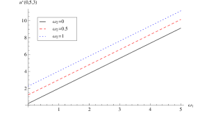
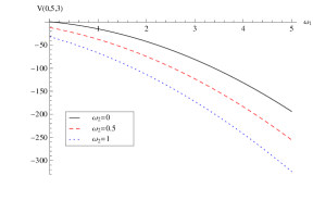
(a) $t=0$

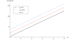
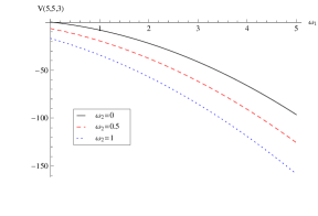
(b) $t=5$

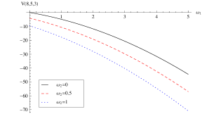
(c) $t=8$

Figure 5.1: Equilibrium strategy and equilibrium value function versus $\omega_{1}$

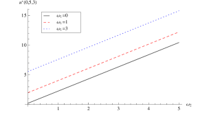
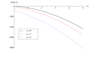
(a) $t=0$

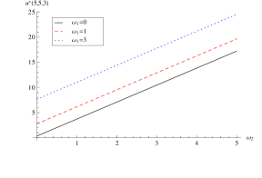
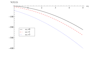
(b) $t=5$

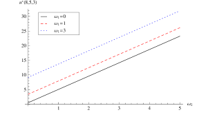
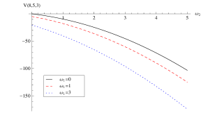
(c) $t=8$

Figure 5.2: Equilibrium strategy and equilibrium value function versus $\omega_{2}$

Appendix

Consider a special case of Wei et al. (2012) with one regime, one bound and one risk asset. The equilibrium strategy is given by

$$\hat{u}(t,s,l) = \frac{\beta(t)\rho(t)}{\sigma(t)}\left[1-e^{-\int_{t}^{T}r(y)\mathrm{d}y}b(t)\right]l+\frac{\theta(t)}{\gamma\sigma^{2}(t)}e^{-\int_{t}^{T}r(y)\mathrm{d}y},$$

where $b(t)$ satisfies the linear of ODE:

$$\begin{cases}\dot{b}(t)&=-\left[\alpha(t)-\frac{\theta(t)\beta(t)\rho(t)}{\sigma(t)}\right]b(t)-\left[\eta(t)+\frac{\theta(t)\beta(t)\rho(t)}{\sigma(t)}\right]e^{\int_{t}^{T}r(y)\mathrm{d}y},\\ b(T)&=0.\end{cases}$$

The solution to the above ODE is given by

$$b(t) = e^{\int_{t}^{T}\left[\alpha(y)-\frac{\theta(y)\beta(y)\rho(y)}{\sigma(y)}\right]\mathrm{d}y}\int_{t}^{T}e^{-\int_{z}^{T}\left[\alpha(y)-\frac{\theta(y)\beta(y)\rho(y)}{\sigma(y)}\right]\mathrm{d}y}\left[\eta(z)+\frac{\theta(z)\beta(z)\rho(z)}{\sigma(z)}\right]e^{\int_{z}^{T}r(y)\mathrm{d}y}\mathrm{d}z$$

$$= e^{\int_{t}^{T}r(y)\mathrm{d}y}\int_{t}^{T}\left[\eta(z)+\frac{\theta(z)\beta(z)\rho(z)}{\sigma(z)}\right]e^{\int_{z}^{t}\left[\eta(y)+\frac{\theta(y)\beta(y)\rho(y)}{\sigma(y)}\right]\mathrm{d}y}\mathrm{d}z.$$

Now consider the special case of our model with $\omega_{1}=0$. Note that the risk aversion in Wei et al. (2012) is $\gamma=\frac{1}{\omega_{2}}$. Thus we have

$$f_{1}(t) =0,$$

$$f_{3}(t) =\frac{\rho(t)\beta(t)}{\sigma(t)}\left[1-\int_{t}^{T}\left[\eta(z)+\frac{\theta(z)\rho(z)\beta(z)}{\sigma(z)}\right]e^{\int_{z}^{t}\left[\eta(y)+\frac{\theta(y)\rho(y)\beta(y)}{\sigma(y)}\right]\mathrm{d}y}\mathrm{d}z\right]$$

$$=\frac{\rho(t)\beta(t)}{\sigma(t)}\left[1-e^{-\int_{t}^{T}r(y)\mathrm{d}y}b(t)\right],$$

$$f_{4}(t) =\frac{\theta(t)}{\gamma\sigma^{2}(t)}e^{-\int_{t}^{T}r(y)\mathrm{d}y}.$$

Thus, in this special case, we get the same equilibrium strategy.

References

• Björk and Murgoci [2010] T. Björk and A. Murgoci. A general theory of Markovian time inconsistent stochastic control problems. Working Paper, Stockholm School of Economics, 2010.
• Björk et al. [2012] T. Björk, A. Murgoci, and X.Y. Zhou. Mean-variance portfolio optimization with state-dependent risk aversion. Mathematical Finance, 2012. To appear.
• Chen and Yang [2011] P. Chen and H. Yang. Markowitz’s mean-variance asset-liability management with regime switching: A multi-period model. Applied Mathematical Finance, 18(1):29–50, 2011.
• Chen et al. [2008] P. Chen, H. Yang, and G. Yin. Markowitz’s mean-variance asset-liability management with regime switching: A continuous-time model. Insurance: Mathematics and Economics, 43:456–465, 2008.
• Chiu and Li [2006] M. C. Chiu and D. Li. Asset and liability management under a continuous-time mean-variance optimization framework. Insurance: Mathematics and Economics, 39:330–355, 2006.
• Ekeland and Lazrak [2006] I. Ekeland and A. Lazrak. Being serious about non-commitment: subgame perfect equilibrium in continuous time. Preprint. University of British Columbia, 2006.
• Ekeland and Pirvu [2008] I. Ekeland and T.A. Pirvu. Investment and consumption without commitment. Mathematics and Financial Economics, 2(1):57–86, 2008.
• Hu et al. [2012] Y. Hu, H. Jin, and X. Y. Zhou. Time-inconsistent stochastic linear-quadratic control. SIAM Journal on Control and Optimization, 50(3):1548–1572, 2012.
• Keel and Müller [1995] A. Keel and H. Müller. Efficient portfolios in the asset liability context. Astin Bulletin, 25:33–48, 1995.
• Leippold et al. [2004] M. Leippold, F. Trojani, and P. Vanini. A geometric approach to multi-period mean variance optimization of assets and liabilities. Journal of Economic Dynamics and Control, 28:1079–1113, 2004.
• Li and Ng [2000] D. Li and W. Ng. Optimal dynamic portfolio selection: Multi-period mean-variance formulation. Mathematical Finance, 10:387–406, 2000.
• Markowitz [1952] H. Markowitz. Portfolio selection. Journal of Finance, 7:77–91, 1952.
• Samuelson [1969] P. A. Samuelson. Lifetime portfolio selection by dynamic stochastic programming. Rev. Econ. Statist., 51:239–246, 1969.
• Sharpe and Tint [1990] W.F. Sharpe and L.G. Tint. Liabilities-a new approach. Journal of Portfolio Management, 16:5–10, 1990.
• Strotz [1955] R. Strotz. Myopia and inconsistency in dynamic utility maximization. Rev. Econ. Stud., 23:165–180, 1955.
• Wei et al. [2012] J.Q. Wei, K.C. Wong, S.C.P. Yam, and S.P. Yung. Markowitz’s mean-variance asset-liability management with regime switching: A time-consistent approach. Preprint, 2012.
• Zhou and Li [2000] X.Y. Zhou and D. Li. Continuous-time mean-variance portfolio selection: A stochastic LQ framework. Appl. Math. Optim., 42:19–33, 2000.