Constrained $\gamma Z$ interference corrections to parity-violating electron scattering

Abstract

We present a comprehensive analysis of $\gamma Z$ interference corrections to the weak charge of the proton measured in parity-violating electron scattering, including a survey of existing models and a critical analysis of their uncertainties. Constraints from parton distributions in the deep-inelastic region, together with new data on parity-violating electron scattering in the resonance region, result in significantly smaller uncertainties on the corrections compared to previous estimates. At the kinematics of the $Q_{\text{weak}}\,\,$experiment, we determine the $\gamma Z$ box correction to be $\Re e\,\square_{\gamma Z}^{V}=(5.57\pm 0.36)\times 10^{-3}$. The new constraints also allow precise predictions to be made for parity-violating deep-inelastic asymmetries on the deuteron.

I Introduction

Modern low-energy experiments at the precision frontier provide important alternatives to high-energy tests of the Standard Model currently being performed at the Large Hadron Collider (for recent reviews, see Refs. Sirlin and Ferroglia (2013); Kumar et al. ; Erler and Su (2013)). One such experiment is the parity-violating (PV) elastic electron-proton scattering measurement that was recently carried out by the $Q_{\text{weak}}\,\,$collaboration at Jefferson Lab Armstrong et al. (2012), which aims to determine the proton’s weak charge $Q_{W}^{p}\,$​ to within 4%. At tree level, the weak charge is related to the weak mixing angle, $\sin^{2}\theta_{W}$, by $Q_{W}^{p}=1-4\sin^{2}\theta_{W}$. By scattering low-energy polarized electrons from an unpolarized hydrogen target, $Q_{\text{weak}}\,\,$measured the asymmetry between the cross sections for right- and left-handed electrons,

$$A_{\rm PV} = \frac{\sigma_{+}-\sigma_{-}}{\sigma_{+}+\sigma_{-}},$$ (1)

where $\sigma_{\lambda}$ is the cross section for a right-hand (helicity $\lambda=+1$) or left-hand (helicity $\lambda=-1$) electron. At small four-momentum transfer squared $t$, the asymmetry is related to $Q_{W}^{p}$ by Musolf et al. (1994)

$$A_{\rm PV} = \frac{G_{F}}{4\pi\alpha\sqrt{2}}\,t\,Q_{W}^{p},$$ (2)

where $G_{F}$ is the Fermi constant and $\alpha$ is the fine structure constant. Including radiative corrections, the proton’s weak charge can be written as Erler et al. (2003)

$$Q_{W}^{p} = \left(1+\Delta\rho+\Delta_{e}\right)\left(1-4\sin^{2}\theta_{W}(0)+\Delta_{e}^{{}^{\prime}}\right)+\square_{WW}+\square_{ZZ}+\square_{\gamma Z}(0),$$ (3)

where $\sin^{2}\theta_{W}(0)$ is the weak mixing angle at zero momentum, and the correction terms $\Delta\rho$, $\Delta_{e}$ and $\Delta_{e}^{{}^{\prime}}$ are well understood and have been computed to sufficient levels of precision Erler et al. (2003). Similarly, the work of Refs. Marciano and Sirlin (1983, 1984); Musolf and Holstein (1990) has established that the electroweak box diagrams $\square_{WW}$ and $\square_{ZZ}$ are known within $Q_{\text{weak}}\,\,$uncertainty limits.

Until recently it was also believed that the interference $\gamma Z$ contribution, illustrated in Fig. 1, was known to sufficient accuracy for the $Q_{\text{weak}}\,\,$experiment. This correction is defined in terms of the electroweak amplitudes as Arrington et al. (2011)

$$\square_{\gamma Z}(0) = Q_{W}^{p}\,{\Re e\left({\cal M}_{\gamma}^{*}{\cal M}_{\gamma Z}^{\rm(PV)}\right)\over\Re e\left({\cal M}_{\gamma}^{*}{\cal M}_{Z}^{\rm(PV)}\right)},$$ (4)

where ${\cal M}_{\gamma}$ is the electromagnetic Born amplitude, ${\cal M}_{Z}^{\rm(PV)}$ is the parity-violating part of the Born $Z$ exchange amplitude, and ${\cal M}_{\gamma Z}^{\rm(PV)}$ is the parity-violating part of the $\gamma Z$ interference amplitude (including the contributions with the $\gamma$ and $Z$ interchanged). A groundbreaking contribution was made by Gorchtein and Horowitz Gorchtein and Horowitz (2009), who showed, using a dispersion relations approach, that the $\square_{\gamma Z}\,$term was strongly energy dependent and was much larger at $Q_{\text{weak}}\,\,$energies ($\sim 1$ GeV) than previous estimates had assumed Erler et al. (2003). More importantly, the uncertainty on this correction was such that it could significantly affect the precision aims of the $Q_{\text{weak}}\,\,$measurement.

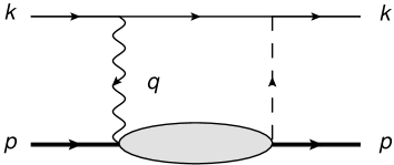
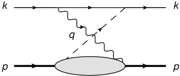
Figure 1: Interference $\gamma Z$ box (left) and crossed box (right) diagrams. The wavy and dashed lines represent the exchanged $\gamma$ and $Z$ bosons, with the electron, hadron and virtual photon momenta labeled by $k$, $p$, and $q$, respectively.

Subsequent analyses by Sibirtsev et al. Sibirtsev et al. (2010) and Rislow and Carlson Rislow and Carlson (2011) generally agreed with the overall scale of the correction found in Ref. Gorchtein and Horowitz (2009), but disputed the magnitude of the uncertainties. In a follow-up study, Gorchtein et al. Gorchtein et al. (2011) performed a more detailed analysis of the model dependence of the $\square_{\gamma Z}\,$contribution, correcting several errors from the original analysis Gorchtein and Horowitz (2009), but still quoted uncertainties twice as large as those in Refs. Sibirtsev et al. (2010); Rislow and Carlson (2011).

Since the interpretation of the $Q_{\text{weak}}\,\,$results depends on having a sound understanding of the $\square_{\gamma Z}\,$correction, the lack of consensus about the magnitude of its uncertainty is obviously problematic. To move beyond this impasse, in this paper we revisit this problem with the aim of resolving the disagreements.

We begin our discussion by outlining in Sec. II the dispersion relation formalism used to compute the $\gamma Z$ corrections in terms of $\gamma Z$ interference structure functions. The latter are the main input into the calculations and are reviewed in detail in Sec. III. In particular, we discuss the uncertainties in determining the $\gamma Z$ structure functions from electromagnetic data for both the resonance and nonresonant background contributions. Constraints from parton distribution functions in the deep-inelastic scattering (DIS) region and new data from the parity-violating electron-deuteron scattering experiment E08-011 at Jefferson Lab Wang et al. (2013) in the resonance region are used in Sec. IV to limit the uncertainty range in models for the $\gamma Z$ structure functions, and to provide more reliable bounds on the box corrections. The resulting $\square_{\gamma Z}^{V}$ correction is presented in Sec. V, where we contrast the revised uncertainties with those estimated in previous unconstrained analyses. Predictions are also made for parity-violating deuteron asymmetries in the deep-inelastic region, as well as for the recently completed inelastic measurement by the $Q_{\text{weak}}\,\,$Collaboration Carlini (2012). Finally, we draw some general conclusions from this analysis in Sec. VI and explore possibilities to further reduce the uncertainties on the $\gamma Z$ corrections in the future.

II Dispersive analysis of parity-violating electron-hadron scattering

The $\gamma Z$ interference correction $\square_{\gamma Z}$ can be decomposed into two parts, arising from the electron vector with hadronic axial-vector coupling to the $Z$ boson ($\square_{\gamma Z}^{A}$) and from the electron axial-vector with vector hadronic coupling to the $Z$ ($\square_{\gamma Z}^{V}$):

$$\square_{\gamma Z}(E) = \square_{\gamma Z}^{A}(E)\ +\ \square_{\gamma Z}^{V}(E).$$ (5)

At very low energies, such as those relevant for atomic parity violation experiments Wood et al. (1997); Dzuba and Flambaum (2012), the $\square_{\gamma Z}^{A}\,$term dominates, while the contribution from the $\square_{\gamma Z}^{V}\,$is negligible. At the energy of the $Q_{\text{weak}}\,\,$experiment, however, both terms provide significant contributions. The $\square_{\gamma Z}^{A}\,$corrections were first computed some time ago by Marciano and Sirlin Marciano and Sirlin (1983, 1984) and were updated recently within a dispersion relation framework by Blunden et al. Blunden et al. (2011, 2012), with reduced errors. The vector hadron correction, $\square_{\gamma Z}^{V}\,$, which is subject to significantly larger uncertainty, will be the focus of the rest of this analysis. We will consider only the inelastic contribution to $\square_{\gamma Z}\,$; the elastic contribution has previously been considered in Refs. Marciano and Sirlin (1983, 1984); Zhou et al. (2007); Tjon et al. (2009) and is strongly suppressed by an additional factor $Q_{W}^{p}$.

For forward scattering, the dispersion relation for the real part of $\square_{\gamma Z}^{V}\,$is given by

$$\Re e\,\square_{\gamma Z}^{V}(E) = \frac{2E}{\pi}{\cal P}\int_{0}^{\infty}dE^{\prime}{1\over E^{\prime 2}-E^{2}}\,\Im m\,\square_{\gamma Z}^{V}(E^{\prime}),$$ (6)

where ${\cal P}$ denotes the principal value integral, and we have used the fact that $\square_{\gamma Z}^{V}\,$is odd under the interchange $E^{\prime}\leftrightarrow-E^{\prime}$. From the optical theorem, the imaginary part of the PV $\gamma Z$ exchange amplitude can be written as Gorchtein and Horowitz (2009); Sibirtsev et al. (2010); Arrington et al. (2011)

$$2\,\Im m\,{\cal M}_{\gamma Z}^{\rm(PV)} = -4\sqrt{2}\pi MG_{F}\int\!\!{d^{3}k^{\prime}\over(2\pi)^{3}2E_{k^{\prime}}}\left({4\pi\alpha\over Q^{2}}\right){1\over 1+Q^{2}/M_{Z}^{2}}\,L_{\mu\nu}^{\gamma Z}\,W^{\mu\nu}_{\gamma Z},$$ (7)

where $Q^{2}=-q^{2}$ represents the virtuality of the exchanged boson, and the integration variable $k^{\prime}=k-q$. The $\gamma Z$ lepton tensor is given by

$$L_{\mu\nu}^{\gamma Z} = \bar{u}(k,\lambda)\,(g_{V}^{e}\gamma_{\mu}-g_{A}^{e}\gamma_{\mu}\gamma_{5})\!\not\!k^{\prime}\,\gamma_{\nu}\,u(k,\lambda),$$ (8)

where the vector and axial-vector couplings of the electron to the weak current are $g^{e}_{V}=-(1-4\sin^{2}\theta_{W})/2$ and $g^{e}_{A}=-1/2$, respectively, and $\lambda$ is the lepton helicity. The hadronic tensor for a nucleon initial state is defined as

$$W^{\mu\nu}(p,q)\ = {1\over 2M}\sum_{X}\langle N(p)|J^{\mu}(0)|X(p_{X})\rangle\langle X(p_{X})|J^{\nu}(0)|N(p)\rangle(2\pi)^{3}\delta^{(4)}(q+p-p_{X}),$$ (9)

where $J_{\gamma}^{\mu}$ and $J_{Z}^{\mu}$ are the electromagnetic and weak neutral currents, respectively, and $p_{X}$ is the four-momentum of the hadronic intermediate state $X$. Using isospin symmetry, the matrix elements of the vector component of the $Z$ current for a proton target can be related to the proton and neutron matrix elements of the electromagnetic current by

$$\langle X|J_{Z}^{\mu}\,|p\rangle = (1-4\sin^{2}\theta_{W})\langle X|J_{\gamma}^{\mu}\,|p\rangle\ -\ \langle X|J_{\gamma}^{\mu}\,|n\rangle,$$ (10)

neglecting the small contribution from strange quarks. In general, the hadronic tensor can be decomposed in terms of the $\gamma Z$ interference structure functions $F_{i}^{\gamma Z}$ as

$$MW^{\mu\nu}_{\gamma Z}\ = -g^{\mu\nu}F_{1}^{\gamma Z}+{p^{\mu}p^{\nu}\over p\cdot q}F_{2}^{\gamma Z}-i\epsilon^{\mu\nu\lambda\rho}{p_{\lambda}q_{\rho}\over 2p\cdot q}F_{3}^{\gamma Z},$$ (11)

where $p$ is the four-momentum of the target hadron. Note that the structure functions $F_{1}^{\gamma Z}$ and $F_{2}^{\gamma Z}$ contribute to the vector hadron contribution, while the $F_{3}^{\gamma Z}$ structure function appears only in the axial-vector hadron correction. Combining Eqs. (8) and (11), the imaginary part of the $\square_{\gamma Z}^{V}$ correction becomes Gorchtein and Horowitz (2009); Sibirtsev et al. (2010); Arrington et al. (2011)

$$\Im m\,\square_{\gamma Z}^{V}(E) = {1\over(s-M^{2})^{2}}\int_{W_{\pi}^{2}}^{s}dW^{2}\int_{0}^{Q^{2}_{\rm max}}dQ^{2}\,{\alpha(Q^{2})\over 1+Q^{2}/M_{Z}^{2}}$$ (12)

$$\hskip 128.0374pt\times\left[F_{1}^{\gamma Z}+{s\left(Q^{2}_{\rm max}-Q^{2}\right)\over Q^{2}\left(W^{2}-M^{2}+Q^{2}\right)}F_{2}^{\gamma Z}\right],$$

where $s=M^{2}+2ME$ is the total center of mass energy squared, $W_{\pi}^{2}=(M+m_{\pi})^{2}$ is the mass at the pion threshold, and $Q^{2}_{\rm max}=2ME(1-W^{2}/s)$. Following Ref. Blunden et al. (2011), we include in Eq. (12) the $Q^{2}$ dependence in $\alpha(Q^{2})$ arising from vacuum polarization contributions.

The most important inputs into Eq. (12) are the $\gamma Z$ interference structure functions $F_{i}^{\gamma Z}$, which are functions of two variables, usually taken to be $Q^{2}$ and the Bjorken scaling variable $x=Q^{2}/2p\cdot q$, or alternatively $Q^{2}$ and $W^{2}$. Unfortunately, these functions are not well determined experimentally. Although there are some data on $F_{1}^{\gamma Z}$ and $F_{2}^{\gamma Z}$ at high $W$ and $Q^{2}$, in the low-$W$ and $Q^{2}$ region, which is crucial to the dispersion integrals, there is little or no information. Unlike the electromagnetic structure functions, which can be fit to the ample data available, the $F_{i}^{\gamma Z}$ must be expressed through models. Given that it can be difficult to resolve the accuracy of the models, the controversy in the literature over the $\Re e\,\square_{\gamma Z}^{V}\$contribution is not surprising.

For later reference, we note here that the $F_{1}$ and $F_{2}$ structure functions, for either $\gamma Z$ or electromagnetic ($\gamma\gamma$) scattering, can be related to the transverse ($\sigma_{T}$) and longitudinal ($\sigma_{L}$) electroweak boson production cross sections as

$$F_{1}(W^{2},Q^{2}) = \left(\frac{W^{2}-M^{2}}{8\pi^{2}\alpha}\right)\sigma_{T}(W^{2},Q^{2}),$$ (13a)

$$F_{2}(W^{2},Q^{2}) = \left(\frac{W^{2}-M^{2}}{8\pi^{2}\alpha}\right)\frac{\nu}{M(1+\nu^{2}/Q^{2})}\left[\sigma_{T}(W^{2},Q^{2})+\sigma_{L}(W^{2},Q^{2})\right],$$ (13b)

where $\nu=E-E^{\prime}$ is the energy transfer. For convenience one often defines the longitudinal structure function as the combination of $F_{1}$ and $F_{2}$ structure functions given by

$$F_{L} = \left(1+\frac{Q^{2}}{\nu^{2}}\right)F_{2}\ -\ 2xF_{1},$$ (14)

where the prefactor can also be written as $(1+4x^{2}M^{2}/Q^{2})$.

III $\gamma Z$ interference structure functions

Most of the uncertainty in the calculation of the $\square_{\gamma Z}\,$correction arises from the incomplete knowledge of the $\gamma Z$ structure functions. There have been extractions of $F_{2}^{\gamma Z}$ and $xF_{3}^{\gamma Z}$ from neutral current DIS by the H1 Collaboration at DESY Aaron et al. (2012) at very high $Q^{2}$ ($60<Q^{2}<50,000$ GeV²) and small $x$ ($0.0008<x<0.65$) using longitudinally polarized lepton beams at HERA. However, these data have little overlap with the region of most relevance for the dispersion integral, which receives contributions primarily from high $x$ and low $Q^{2}$, where there are no direct measurements. Consequently, one must appeal to models of the interference structure functions to estimate $\square_{\gamma Z}\,$.

In this section we review the models used in the literature for the $\gamma Z$ structure functions, before presenting our constrained model, which we refer to as the Adelaide-Jefferson Lab-Manitoba (AJM) model. The construction of the models involves first choosing appropriate electromagnetic structure functions $F_{i}^{\gamma\gamma}$, and then transforming these to the $\gamma Z$ case. In describing the structure functions, or equivalently the virtual boson-proton cross sections $\sigma_{T,L}$ in Eqs. (13), it is convenient to separate the full range of kinematics into a resonance part and a smooth nonresonant background,

$$\sigma_{T,L} = \sigma_{T,L}^{\rm(res)}+\sigma_{T,L}^{\rm(bgd)}.$$ (15)

The $\sigma_{T,L}^{\rm(res)}$ term includes a sum over the prominent low-lying resonances, while $\sigma_{T,L}^{\rm(bgd)}$ is determined phenomenologically by fitting the inclusive scattering data Christy and Bosted (2010); Bosted and Christy (2008). Although such a separation is inherently model dependent, as only the total cross section is physical, it nevertheless provides a useful way to parametrize the somewhat different behaviors of the cross sections in the low- and high-$W$ regions.

For completeness, the following list summarizes the models for the $\gamma Z$ structure functions that have been discussed in the literature:

1. color-dipole model Cvetic et al. (2001, 2000), referred to as “Model I” in Gorchtein et al. (GHRM) Gorchtein et al. (2011);

2. vector meson dominance (VMD) + Regge model Sakurai and Schildknecht (1972); Alwall and Ingelman (2004), referred to as “Model II” by GHRM Gorchtein et al. (2011);

3. Sibirtsev et al. (SBMT) model Sibirtsev et al. (2010), based on the Regge parametrization of Capella et al. Capella et al. (1994);

4. Carlson and Rislow (CR) model Carlson and Rislow (2012); Rislow and Carlson (2011).

The models Gorchtein et al. (2011); Sibirtsev et al. (2010); Rislow and Carlson (2011); Carlson and Rislow (2012) differ primarily in the treatment of the background contributions $\sigma_{T,L}^{\rm(bgd)}$ for the $\gamma Z$ interference, the uncertainty on which is the main source of disagreement between the various estimates of $\square_{\gamma Z}\,$. For the resonance region, all of the models (with the exception of SBMT Sibirtsev et al. (2010)) use the Christy and Bosted (CB) parametrization Christy and Bosted (2010) of the electromagnetic structure functions at low $W$, but differ in how these are transformed to the $\gamma Z$ case. Note, however, in both Model I and Model II of GHRM some of the resonance parameters in the CB fit are modified to better match the choice of background contribution Gorchtein et al. (2011). In the following we discuss both the resonance and background content of these models in more detail.

III.1 Resonances

The CB parametrization Christy and Bosted (2010) of $F_{1,2}^{\gamma\gamma}$ fits the resonance region electron-proton scattering data in terms of the seven most important resonances ($P_{33}(1232)$, $P_{11}(1440)$, $D_{13}(1520)$, $S_{11}(1535)$, $S_{15}(1650)$, $F_{15}(1680)$ and an $l=3$ state with mass 1934 MeV), and generally agrees with the data to within $5\%$. The CB fit is used as the basis for the resonance models of Carlson and Rislow Carlson and Rislow (2012), and Gorchtein et al. Gorchtein et al. (2011), with the latter using slightly modified parameters for $\sigma_{T,L}^{\rm(res)}$ in their Models I and II. Sibirtsev et al. Sibirtsev et al. (2010), on the other hand, perform their own fit of the data, incorporating the four resonances $P_{33}(1232)$, $D_{13}(1520)$, $F_{15}(1680)$ and $F_{37}(1950)$, and also obtain a reasonably good description of the data.

Modifying the electromagnetic structure functions to obtain their interference analogs involves modifying the contribution from each resonance $R$ by a ratio that takes into account the differences between the electromagnetic and weak neutral transition amplitudes, according to Eq. (10). For the transverse cross section GHRM define this ratio for a proton as Gorchtein et al. (2011)

$$\xi_{R} \equiv \frac{\sigma_{T,R}^{\gamma Z}}{\sigma_{T,R}^{\gamma\gamma}}\ =\ (1-4\sin^{2}\theta_{W})-y_{R},$$ (16)

where

$$y_{R}=\frac{A_{R,\frac{1}{2}}^{p}\,A_{R,\frac{1}{2}}^{n^{*}}+A_{R,\frac{3}{2}}^{p}\,A_{R,\frac{3}{2}}^{n^{*}}}{\big{|}A_{R,\frac{1}{2}}^{p}\big{|}^{2}+\big{|}A_{R,\frac{3}{2}}^{p}\big{|}^{2}},$$ (17)

with $A_{R,\lambda}^{N}$ the transition amplitude from a proton or neutron to a resonance $R$ with helicity $\lambda=\frac{1}{2}$ or $\frac{3}{2}$. The amplitudes $A_{R,\lambda}^{N}$ are assumed by GHRM to be $Q^{2}$ independent, and their values determined from electromagnetic decays at $Q^{2}=0$ Nakamura et al. (2010). The ratio for the longitudinal cross section is taken to be equal to the transverse ratio in both Models I and II of GHRM.

Carlson and Rislow Carlson and Rislow (2012) use a similar ratio to that in Eq. (16) (which they label as $C_{R}$), but include in addition a $Q^{2}$ dependence in the amplitudes derived from the MAID unitary isobar model Tiator et al. (2011). For comparison, CR also calculate the transition amplitudes using a constituent quark model Rislow and Carlson (2011).

Finally, Sibirtsev et al. Sibirtsev et al. (2010) use the conservation of the vector current and isospin symmetry to set the ratio for isospin-3/2 states to $(1+Q_{W}^{p})\approx(2-4\sin^{2}\theta_{W})$. For the isospin-1/2 resonances, such as the $D_{13}(1520)$, SU(6) quark model wave functions are used to estimate the ratio of couplings. The similarity of the magnitudes of the weak and electromagnetic couplings was used by SBMT to justify approximating the ratio $\xi_{R}$ by 1.

III.2 Background

III.2.1 Electromagnetic structure functions

Although the CB parametrization Christy and Bosted (2010) includes a background $\sigma_{T,L}^{\rm(bgd)}$ at low $W$ ($W<3$ GeV), to describe the nonresonant contributions to the electromagnetic structure functions at $W>3$ GeV requires a model for the background which is also valid at large $W$. In the calculation of GHRM Gorchtein et al. (2011), the color dipole model from Cvetic et al. Cvetic et al. (2001, 2000) is used for Model I, while the VMD+Regge model of Alwall and Ingelman Alwall and Ingelman (2004) is employed for Model II. Since the latter was shown by GHRM to introduce the largest uncertainty in $\square_{\gamma Z}\,$, it will be the main focus of our attention.

According to the VMD hypothesis, the interaction of a photon $\gamma$ with a hadron proceeds through transitions to vector mesons $V$ (with $V=\rho$, $\omega$ or $\phi$), with strength $\sqrt{4\pi\alpha}/f_{V}$, where $f_{V}$ is the electromagnetic decay constant of $V$. The three vector mesons saturate around 80% of the total photoproduction cross section Sakurai and Schildknecht (1972). The remainder is usually attributed to contributions from higher masses, which are modeled by a continuum of states starting at mass $m_{0}\approx 1.4$ GeV Sakurai and Schildknecht (1972). (In the case of the color dipole model Cvetic et al. (2001, 2000); Kuroda and Schildknecht (2012), the photon is assumed to interact with the hadron through coupling to uncorrelated $q\bar{q}$ states instead of mesons.) Following Ref. Alwall and Ingelman (2004), we neglect the off-diagonal terms in the mass integral, which is known to be a good approximation for scattering from nucleons Fraas et al. (1975). The transverse and longitudinal virtual photon-nucleon cross sections can then be expressed as Alwall and Ingelman (2004)

$$\sigma_{T}^{\rm VMD} = \sigma_{\gamma N}\Bigg{[}\sum_{V}\,r_{V}\frac{1}{(1+Q^{2}/m_{V}^{2})^{2}}\ +\ r_{C}\,\frac{1}{1+Q^{2}/m_{0}^{2}}\Bigg{]},$$ (18a)

$$\sigma_{L}^{\rm VMD} = \sigma_{\gamma N}\Bigg{[}\sum_{V}\,r_{V}\,\xi_{V}\,\frac{Q^{2}/m_{V}^{2}}{(1+Q^{2}/m_{V}^{2})^{2}}$$ (18b)

$$\hskip 28.45274pt+\ r_{C}\,\xi_{C}\left(\frac{m_{0}^{2}}{Q^{2}}\ln(1+Q^{2}/m_{0}^{2})-\frac{1}{1+Q^{2}/m_{0}^{2}}\right)\Bigg{]},$$

where $\sigma_{\gamma N}$ is the real photon-nucleon cross section, and the constants $r_{V}\sim 1/f_{V}^{2}$ represent the relative contributions from the individual vector mesons $V$, with $r_{C}=1-\sum\limits_{V}r_{V}$ being the continuum fraction Alwall and Ingelman (2004). Phenomenologically, the $r_{V}$ values are determined as $r_{V}=\left\{0.67,\,0.062,\,0.059\right\}$ for $V=\rho$, $\omega$ and $\phi$, respectively Bauer et al. (1978). As we shall see below, $r_{C}$ plays a critical role in determining the uncertainty on the interference cross sections. The parameters $\xi_{V}$ and $\xi_{C}$ allow for different behavior of the transverse and longitudinal components of the vector mesons, although in practice these are usually set equal, $\xi_{V}=\xi_{C}$, in order to fit the available data. Note that despite the apparent $1/Q^{2}$ dependence in the second term of $\sigma_{L}^{\rm VMD}$ in Eq. (18b), one can verify by expanding the logarithm for small $Q^{2}$ that the longitudinal cross section does in fact vanish in the $Q^{2}\to 0$ limit. According to Regge theory, the real photon cross section can be parametrized as a sum of two terms Donnachie and Landshoff (1992),

$$\sigma_{\gamma N} = A_{\gamma}\,s_{\gamma}^{\epsilon}+B_{\gamma}\,s_{\gamma}^{-\eta},$$ (19)

where $s_{\gamma}\equiv W^{2}$, with the exponents $\epsilon$ and $\eta$ giving the energy dependence of the Pomeron and Reggeon terms, which have coefficients $A_{\gamma}$ and $B_{\gamma}$, respectively.

In the model of SBMT, the background is parametrized according to the structure function fit of Capella et al. Capella et al. (1994), with several parameters adjusted to better describe recent data, as discussed in Ref. Sibirtsev et al. (2010). The parametrization of the $F_{2}^{\gamma\gamma}$ structure function, which is valid for all $Q^{2}$, is again given by a sum of Pomeron ($P$) and Reggeon $R$ exchange terms,

$$F_{2}^{\gamma\gamma}(x,Q^{2}) = A_{\rm P}\,x^{-\Delta}(1-x)^{n+4}\left[\frac{Q^{2}}{Q^{2}+\Lambda_{\rm P}^{2}}\right]^{1+\Delta}\ +\ A_{\rm R}\,x^{1-\alpha_{\rm R}}(1-x)^{n}\left[\frac{Q^{2}}{Q^{2}+\Lambda_{\rm R}^{2}}\right]^{\alpha_{\rm R}},$$

where $\Delta$ and $n$ are both functions of $Q^{2}$, and $A_{\rm P}$, $\Lambda_{\rm P}$, $A_{\rm R}$, $\Lambda_{\rm R}$ and $\alpha_{\rm R}$ are fit parameters Capella et al. (1994). The $F_{1}^{\gamma\gamma}$ structure function is obtained by SBMT from a parametrization of the ratio of longitudinal to transverse cross sections. From Eqs. (13) this can be written as

$$\frac{\sigma_{L}}{\sigma_{T}} = \left(1+\frac{4M^{2}x^{2}}{Q^{2}}\right)\frac{F_{2}}{2xF_{1}}-1,$$ (21)

which is parametrized by a sum of exponentials Sibirtsev et al. (2010).

While the above models use the same background parametrization over the entire range of kinematics, CR Rislow and Carlson (2011); Carlson and Rislow (2012) on the other hand divide their dispersion integral into three distinct regions, each described by a different model. In particular, the resonance region at low $W$ is described in terms of the CB fit to $\sigma_{T,L}^{\rm(res)}$ and $\sigma_{T,L}^{\rm(bgd)}$ Christy and Bosted (2010), while for the high-$W$, low-$Q^{2}$ region, CR use the Capella et al. structure function parametrization. For high $W$ and high $Q^{2}$, a partonic description is employed using the CT10 global fit Lai et al. (2010) of parton distribution functions (PDFs).

III.2.2 $\gamma Z$ structure functions

To construct the nonresonant background contributions to the transverse and longitudinal $\gamma Z$ cross sections, the electromagnetic cross sections need to be rescaled by the ratio $\sigma_{T,L}^{\gamma Z}/\sigma_{T,L}^{\gamma\gamma}$, as for the resonance components. For Model II of GHRM Gorchtein et al. (2011), a generalization of the VMD model is used, assuming the $\gamma Z$ cross section for vector meson $V$ is given by the analogous $\gamma\gamma$ cross section scaled by the ratio $\kappa_{V}$ of weak and electric charges,

$$\sigma_{T,L}^{\gamma Z(V)} = \kappa_{V}\,\sigma_{T,L}^{\gamma\gamma(V)},$$ (22)

where

$$\kappa_{\rho} = 2-4\sin^{2}\theta_{W},$$ (23a)

$$\kappa_{\omega} = -4\sin^{2}\theta_{W},$$ (23b)

$$\kappa_{\phi} = 3-4\sin^{2}\theta_{W}$$ (23c)

correspond to the isovector, isoscalar and strange quark components of the electroweak current, respectively. This allows the ratio of $\gamma Z$ to $\gamma\gamma$ cross sections to be written as Gorchtein et al. (2011)

$$\frac{\sigma_{T,L}^{\gamma Z}}{\sigma_{T,L}^{\gamma\gamma}}=\frac{\kappa_{\rho}+\kappa_{\omega}\,R_{\omega}^{T,L}(Q^{2})+\kappa_{\phi}\,R_{\phi}^{T,L}(Q^{2})+\kappa_{C}^{T,L}\,R_{C}^{T,L}(Q^{2})}{1+R_{\omega}^{T,L}(Q^{2})+R_{\phi}^{T,L}(Q^{2})+R_{C}^{T,L}(Q^{2})},$$ (24)

where $R_{V}^{T,L}$ is the ratio of cross sections for $V$ and the $\rho$ meson,

$$R_{V}^{T,L} \equiv \frac{\sigma_{T,L}^{\gamma\gamma(V)}}{\sigma_{T,L}^{\gamma\gamma(\rho)}}\ =\ \frac{f_{\rho}^{2}}{f_{V}^{2}}\left(\frac{1+Q^{2}/m_{\rho}^{2}}{1+Q^{2}/m_{V}^{2}}\right)^{2}.$$ (25)

The corresponding ratio $R_{C}^{T,L}$ of the continuum to $\rho$ contributions is given by

$$R_{C}^{T} = \frac{r_{C}}{r_{\rho}}\left(\frac{1+Q^{2}/m_{\rho}^{2}}{1+Q^{2}/m_{0}^{2}}\right)^{2},$$ (26a)

$$R_{C}^{L} = \frac{r_{C}}{r_{\rho}}\left[\frac{m_{0}^{2}}{Q^{2}}\ln(1+Q^{2}/m_{0}^{2})\ -\ \frac{1}{1+Q^{2}/m_{0}^{2}}\right]\Big{/}\left[\frac{Q^{2}/m_{\rho}^{2}}{(1+Q^{2}/m_{\rho}^{2})^{2}}\right],$$ (26b)

with the continuum mass parameter set to $m_{0}=1.5$ GeV Gorchtein et al. (2011). The parameters $\kappa_{C}^{T,L}$ in Eq. (24) denote the ratios of the $\gamma Z$ and $\gamma\gamma$ continuum contributions to the cross section. Unlike for the discrete vector meson terms, the VMD model does not prescribe a simple charge ratio factor to modify the continuum part of the cross section. In view of this, GHRM proceed by assigning a 100% uncertainty on this contribution. As we will see below, this assumption gives the largest contribution to the uncertainty on $\square_{\gamma Z}\,$.

For Model I of GHRM, the same general form for the $\gamma Z$ cross sections is used as in Eq. (24), but with different individual contributions $R_{V}^{T,L}$. Whereas in Model II, the $R_{V}^{T,L}$ are functions of $Q^{2}$, in Model I these become constants with relative strengths determined by squares of quark electric charges, with the continuum contribution associated with the $J/\psi$ meson Gorchtein et al. (2011), $\{\rho:\omega:\phi:J/\psi\}=\{1:1/9:2/9:8/9\}$. Similarly, a 100% uncertainty is assumed for the $J/\psi$ term in Model I.

In the SBMT model Sibirtsev et al. (2010), the $\gamma Z$ structure functions at low $x$ are approximated by their electromagnetic counterparts. This is motivated by the approximate flavor independence of sea quark distributions in the low-$x$ region, and the similarity of the sum of the electroweak couplings for three quark flavors, $\left(\sum_{q}e_{q}\,g_{V}^{q}\right)/\left(\sum_{q}e_{q}^{2}\right)=2-4\sin^{2}\theta_{W}\approx 1$ Gorchtein and Horowitz (2009), where $e_{q}$ and $g_{V}^{q}$ are the electric and weak vector charges of quark $q$, respectively. At larger $x$ ($x\gtrsim 0.4$), however, SBMT compute $F_{i}^{\gamma Z}$ using a ratio of leading twist (LT) structure functions computed from the Martin-Roberts-Stirling-Thorne parton distribution functions Martin et al. (2003),

$$F_{i}^{\gamma Z} = \left(\frac{F_{i}^{\gamma Z}}{F_{i}^{\gamma\gamma}}\right)^{\rm LT}F_{i}^{\gamma\gamma}.$$ (27)

At these $x$ values, SBMT note that the flavor dependence of the parton distributions renders the interference function approximately $30\%\!-\!40\%$ smaller than the electromagnetic one. The functions $F_{i}^{\gamma\gamma}$ therefore provide an upper limit on $F_{i}^{\gamma Z}$.

Finally, for the CR model Carlson and Rislow (2012); Rislow and Carlson (2011) the method for modifying the $\gamma\gamma$ background cross sections depends on the kinematic region of $W$ and $Q^{2}$. In the resonance region, CR take the average of the high energy ($x\to 0$) limit ($u=d=s$), in which $F_{i}^{\gamma Z}/F_{i}^{\gamma\gamma}=2-4\sin^{2}\theta_{W}$, and the SU(6) quark limit ($u=2d,s=0$), in which $F_{i}^{\gamma Z}/F_{i}^{\gamma\gamma}=5/3-4\sin^{2}\theta_{W}$, to convert the electromagnetic background from the CB structure function parametrization Christy and Bosted (2010). For the low-$Q^{2}$, high-$W$ region, CR apply the same ratio to the Capella et al. Capella et al. (1994) parametrization as SBMT, while in the DIS region they compute the $F_{i}^{\gamma Z}$ structure functions directly from LT parton distributions Lai et al. (2010).

Using these models for the resonance and nonresonant background contributions to the $\gamma Z$ structure functions, the analyses of GHRM Gorchtein et al. (2011), SBMT Sibirtsev et al. (2010) and CR Rislow and Carlson (2011) estimate the $\square_{\gamma Z}\,$correction at the $Q_{\text{weak}}\,\,$energy to be

$$\Re e\,\square_{\gamma Z}^{V} = (5.4\pm 2.0)\times 10^{-3}\hskip 56.9055pt{\rm[GHRM]}$$ (28a)

$$\Re e\,\square_{\gamma Z}^{V} = (4.7_{\ -0.4\,}^{\ +1.1\,})\times 10^{-3}\hskip 64.01869pt{\rm[SBMT]}$$ (28b)

$$\Re e\,\square_{\gamma Z}^{V} = (5.7\pm 0.9)\times 10^{-3}\hskip 56.9055pt{\rm[CR]}$$ (28c)

respectively. The GHRM result for the central value of $\Re e\,\square_{\gamma Z}^{V}\$is the average of Models I and II, but with the dominant background error taken from the larger of the two, in this case Model II. The GHRM analysis also estimates the effect of the $t$ dependence of the $\square_{\gamma Z}\,$correction, from $t=0$ in the dispersion formalism to $t=-0.03$ GeV² in the $Q_{\text{weak}}\,\,$experiment, finding a decrease of approximately 1.3%, with a similar uncertainty on the correction at the $Q_{\text{weak}}\,\,$point.

The central values of all the calculations agree within the quoted uncertainties; however, the error on the GHRM value is twice as large as those on the SBMT and CR calculations, even though the SBMT estimate includes a fairly conservative uncertainty on the input $\gamma\gamma$ structure functions. Given the importance of the $\square_{\gamma Z}\,$correction to the extraction of the weak mixing angle from the $Q_{\text{weak}}\,\,$measurement, it is vital that the origin of this difference be understood, and ways of further reducing the uncertainty explored.

III.3 Adelaide-Jefferson Lab-Manitoba model

To proceed with our analysis of the $\gamma Z$ correction, we define here the ingredients of our AJM model, within which we will study in detail the various contributions to $\Re e\,\square_{\gamma Z}^{V}\$and their uncertainties. We draw on the valuable experience obtained with the existing models Gorchtein and Horowitz (2009); Gorchtein et al. (2011); Sibirtsev et al. (2010); Rislow and Carlson (2011); Carlson and Rislow (2012), and incorporate into the AJM model some of the more robust features of the previous analyses. Most importantly, we consider additional constraints from existing data on some of the model parameters which were unconstrained in the earlier work. We will find that indeed data on PDFs near the resonance-DIS transition, together with new results on inclusive parity-violating electron scattering asymmetries, place significant constraints on the models, in particular on the background contribution.

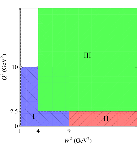
Figure 2: (color online) Kinematic regions contributing to the $\square_{\gamma Z}^{V}\,$integrals in the AJM model: Region I (blue shaded) at low $W$ and low $Q^{2}$ is described by the CB $F_{1,2}^{\gamma\gamma}$ fit Christy and Bosted (2010), transformed to the $\gamma Z$ case; Region II (red shaded) represents the high-$W$, low-$Q^{2}$ domain as in Ref. Alwall and Ingelman (2004) (or the GHRM Model II Gorchtein et al. (2011)), transformed to $\gamma Z$; and Region III (green shaded) at high $W$ and high $Q^{2}$ is described by global PDF fits to high-energy scattering data Alekhin et al. (2012).

III.3.1 $\gamma\gamma$ structure functions

Following CR Rislow and Carlson (2011); Carlson and Rislow (2012), we divide the integrals in Eq. (12) into distinct regions of $W^{2}$ and $Q^{2}$, using specific models to parametrize the $\gamma Z$ structure functions in each region. This is illustrated in Fig. 2, where the $W^{2}$ and $Q^{2}$ divisions and the models describing them are indicated. Although the boundaries between the regions are clearly defined, the models themselves overlap, allowing important checks to be made on the continuity of the descriptions across the boundaries.

Figure 3: (color online) Proton $F_{2}^{\gamma\gamma}$ structure function versus $W^{2}$ at fixed $Q^{2}=0.05$, 0.5, 1.5 and 2 GeV² for the CB fit Christy and Bosted (2010) at low $W$ (blue solid) and VMD+Regge parametrization Alwall and Ingelman (2004) at high $W$ (red dashed). The boundary between these (corresponding to Regions I and II in Fig. 2) is indicated by the vertical dashed line at $W^{2}=9$ GeV².

For the input $\gamma\gamma$ structure functions, we use the CB parametrization Christy and Bosted (2010) to describe the low-$W$ region (Region I) at $W_{\pi}<W<2$ GeV for all $Q^{2}$ up to 10 GeV². In fact, the strong suppression of the resonance transition form factors with increasing $Q^{2}$ results in negligible resonance contributions already beyond $Q^{2}\approx 2$ GeV². Since the CB fit also describes data up to $W^{2}=9$ GeV², we use it in the higher-$W$ region for $Q^{2}<2.5$ GeV², as indicated by the blue shaded area in Fig. 2.

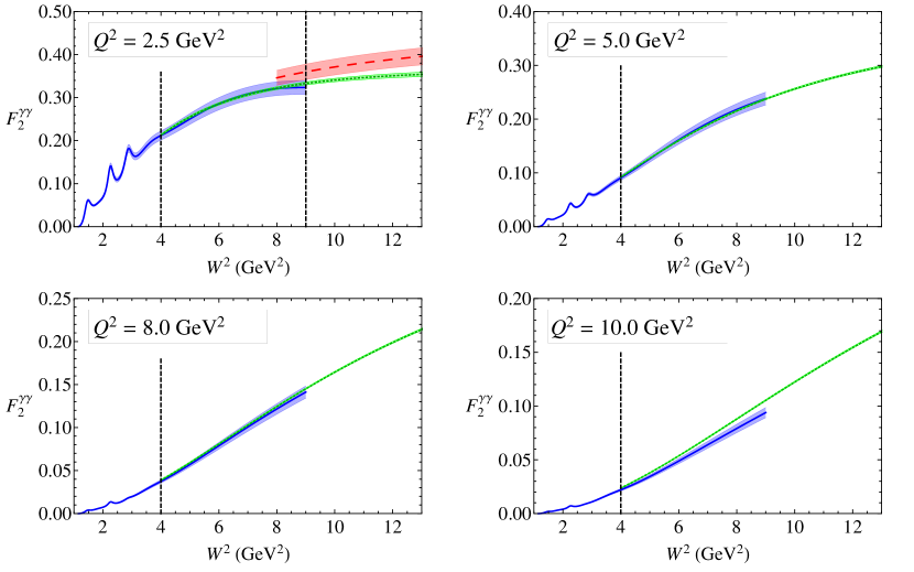
Figure 4: (color online) Proton $F_{2}^{\gamma\gamma}$ structure function versus $W^{2}$ at fixed $Q^{2}=2.5$, 5, 8 and 10 GeV² for the CB fit Christy and Bosted (2010) at low $W$ (blue solid) and the ABM11 PDF parametrization Alekhin et al. (2012) at high $W$ (green dotted), with the boundary between Regions I and III at $W^{2}=4$ GeV² indicated by the vertical line. For the $Q^{2}=2.5$ GeV² panel, the matching with the VMD+Regge model Alwall and Ingelman (2004) (red dashed), corresponding to the boundary between Regions I and II, is indicated by the vertical line at $W^{2}=9$ GeV².

At higher $W$, corresponding to kinematics where Regge theory is applicable, the VMD+Regge model of Alwall and Ingelman Alwall and Ingelman (2004) is combined with a modified CB resonance contribution (cf. Table II of Ref. Gorchtein et al. (2011)) to describe the structure functions for $W^{2}>9$ GeV² and $Q^{2}<2.5$ GeV² (Region II, red shaded area in Fig. 2). Of course, at these values of $W$ the resonances will contribute very little to the dispersion integral in Eq. (12), which will be contaminated by the background contribution. This model also forms the basis for Model II of GHRM Gorchtein et al. (2011). The matching of the CB and VMD+Regge parametrizations at the boundary between the low-$W$ and high-$W$ regions is illustrated in Fig. 3 for the $F_{2}^{\gamma\gamma}$ structure function as a function of $W^{2}$, at several fixed values of $Q^{2}$, from $Q^{2}=0.05$ to 2 GeV². The agreement between the two models in the region of overlap is clearly excellent. For the structure function in the VMD+Regge model, we have assumed a conservative 5% uncertainty, similar to that for the CB parametrization.

In the DIS region at high $W$ and high $Q^{2}$ (green shaded area in Fig. 2), the structure functions can be computed in terms of global PDFs, for which we use the next-to-next-to-leading order (NNLO) fit by Alekhin et al. (ABM11) Alekhin et al. (2012). This fit includes both leading twist and higher twist contributions, allowing for descriptions of data for $Q^{2}>2.5$ GeV² and $W>1.8$ GeV, which overlaps partially with the CB Christy and Bosted (2010) and VMD+Regge Alwall and Ingelman (2004) parametrizations. (Other similar global fits, such as those in Refs. Accardi et al. (2011); Owens et al. (2012); Ball et al. (2010); Jimenez-Delgado and Reya (2009); Martin et al. (2009), give very similar results, and differences between the parametrization generally lie within the PDF uncertainties.) The transition between DIS kinematics (Region III) and the models describing the lower-$W$ and $Q^{2}$ regions is illustrated in Fig. 4 for $F_{2}^{\gamma\gamma}$ at $Q^{2}=2.5$ GeV² (where the transitions between all three parametrizations are shown at $W^{2}=9$ GeV²) and at higher $Q^{2}$ values, up to $Q^{2}=10$ GeV², for the transition between Regions I and III. Again, the models generally match very well across these kinematic boundaries.

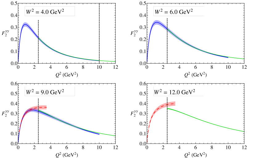
Figure 5: (color online) Proton $F_{2}^{\gamma\gamma}$ structure function versus $Q^{2}$ at fixed $W^{2}=4$, 6, 9 and 12 GeV² for the CB fit Christy and Bosted (2010) (blue solid), the ABM11 PDF parametrization Alekhin et al. (2012) (green dotted), and the VMD+Regge model Alwall and Ingelman (2004) (red dashed), with the boundaries between Regions I, II and III indicated by the vertical lines at fixed $Q^{2}$. Note that the small disagreement between the VMD+Regge model and the PDF parametrization for $Q^{2}=2.5$ GeV² appears only at larger $W^{2}$ values where the contribution to the dispersion integral is small.

The boundaries between the three regions can also be displayed for fixed $W^{2}$ as a function of $Q^{2}$, as illustrated in Fig. 5. The matching of Regions I and II for $W^{2}=4$ GeV² shows excellent agreement between the CB Christy and Bosted (2010) and ABM11 PDF Alekhin et al. (2012) parametrizations at $Q^{2}=2.5$ GeV². At the highest $W$ value at which the CB fit is valid, $W^{2}=9$ GeV², the agreement between the models describing all three regions is also quite good. For larger $W$ ($W^{2}\gtrsim 10$ GeV²) the VMD+Regge model Alwall and Ingelman (2004) slightly exceeds the PDF parametrization. However, this generally occurs at the edge of the kinematic boundary between Regions II and III, where the contribution to the imaginary part of $\square_{\gamma Z}\,$in Eq. (12) is very small.

III.3.2 $\gamma Z$ structure functions

Having detailed the forms of the electromagnetic structure functions, we now turn to their $\gamma Z$ interference analogs. For the low-$W$/low-$Q^{2}$ region dominated by the nucleon resonances, the transverse and longitudinal $\gamma\gamma$ cross sections parametrized in the CB fit Christy and Bosted (2010) are modified using the ratio $\xi_{R}$ in Eq. (16), with the parameter $y_{R}$ determined from the proton and neutron helicity amplitudes as in Eq. (17). This follows closely the approach adopted by GHRM Gorchtein et al. (2011), but, importantly, differs in the way the uncertainties on the helicity amplitudes $A_{R,\lambda}^{N}$ are determined.

In particular, GHRM combined the uncertainties on the amplitudes by adding extremal values of each, which implicitly assumes a uniform error distribution rather than the standard Gaussian one. Adding errors linearly clearly overestimates the uncertainties, and in the AJM analysis we adopt the more conventional Gaussian distribution to add the errors in quadrature. (When combining all of the uncertainties on the final $\Re e\,\square_{\gamma Z}^{V}\$value, however, GHRM add the errors in quadrature.) In Table 1 the $y_{R}$ values for the proton and their uncertainties computed using both methods are shown for comparison. For completeness, we also list the $y_{R}$ values for the neutron and deuteron, with uncertainties added in quadrature, which will be needed in subsequent sections. For the isospin-$\frac{3}{2}$ $P_{33}(1232)$ and $F_{37}(1950)$ resonances, the uncertainties on the helicity amplitudes are given by the Particle Data Group (PDG) Beringer et al. (2012) as zero. To be conservative, however, we follow GHRM Gorchtein et al. (2011) and include a 10% uncertainty on the $P_{33}(1232)$ and a 100% uncertainty on the $F_{37}(1950)$ resonance Christy and Bosted (2010); Bosted and Christy (2008).

Table 1: Electromagnetic to $\gamma Z$ resonance cross section transformation ratios $y_{R}$ from Eq. (17) for the proton, neutron and deuteron in the AJM model, compared with the proton ratio in the GHRM model Gorchtein et al. (2011). The AJM model values in parentheses use helicity amplitudes from the earlier 2010 PDG Nakamura et al. (2010), as utilized by GHRM. The errors labeled with the asterisks $(*)$ are values corrected Gorchtein (2012) from those in Ref. Gorchtein et al. (2011).

		$P_{33}(1232)$		$P_{11}(1440)$		$D_{13}(1520)$		$S_{11}(1535)$		$S_{11}(1665)$		$F_{15}(1680)$		$F_{37}(1950)$
	$p$ (AJM)	$-1.0\pm 0.1$		$-0.67\pm 0.17$		$-0.84\pm 0.17$		$-0.51\pm 0.35$		$-0.28\pm 0.41$		$-0.27\pm 0.08$		$-1\pm 1$
				$(-0.62\pm 0.16)$		$(-0.77\pm 0.08)$
	$p$ (GHRM)	$-1.0\pm 0.1$		$-0.62^{+0.19}_{-0.20}$		$-0.77^{+0.122}_{-0.125}$${}^{\ (*)}$		$-0.51^{+0.35}_{-0.71}$		$-0.28^{+0.45}_{-0.69}$${}^{\ (*)}$		$-0.27^{+0.10}_{-0.12}$		$-1\pm 1$
	$n$ (AJM)	$-1.0\pm 0.1$		$-1.50\pm 0.39$		$-0.85\pm 0.15$		$-1.96\pm 1.32$		$-3.53\pm 5.06$		$-2.50\pm 1.01$		$-1\pm 1$
	$d$ (AJM)	$-1.0\pm 0.1$		$-0.92\pm 0.27$		$-0.85\pm 0.14$		$-0.81\pm 0.64$		$-0.52\pm 0.78$		$-0.49\pm 0.14$		$-1\pm 1$

Note that in Table 1 and in our numerical calculations we make use of the latest values of the helicity amplitudes from the PDG Beringer et al. (2012). However, when comparing directly with the GHRM analysis Gorchtein et al. (2011) we will refer to the earlier, 2010 PDG values Nakamura et al. (2010) that were utilized by GHRM for the $D_{13}(1520)$ and $P_{11}(1440)$ resonances. The $y_{R}$ ratios using these earlier values are listed in parentheses in Table 1, but with errors evaluated using Gaussian distributions.

For the nonresonant background, the models describing the electromagnetic structure functions are transformed to the $\gamma Z$ case according to the kinematic region considered. For the region of low $Q^{2}$ but high $W$, the cross section in the VMD+Regge model Alwall and Ingelman (2004) is modified using the ratio in Eq. (24), in analogy with Model II of GHRM Gorchtein et al. (2011). However, instead of fixing the parameters $\kappa_{C}^{T,L}$ so that the $\gamma\gamma$ and $\gamma Z$ continuum pieces are equal Gorchtein et al. (2011), we allow these to be determined by demanding that the $\gamma Z$ structure functions be continuous across the boundaries of this region, that is, at $W=3$ GeV and $Q^{2}=2.5$ GeV². As we will see in the following section, this places strong constraints on $\kappa_{C}^{T,L}$, leading to significantly reduced uncertainties on the resulting value of $\Re e\,\square_{\gamma Z}^{V}\$.

Finally, the $\gamma Z$ structure functions in the DIS region, at $W^{2}>4$ GeV² and $Q^{2}>2.5$ GeV², are computed from the ABM11 PDF parametrization Alekhin et al. (2012); Alekhin (2012). The transformation from $\gamma\gamma$ to $\gamma Z$ is trivial at the parton level, amounting to a replacement of the quark electric charges $e_{q}$ multiplying the universal PDFs by the weak vector charges $g_{V}^{q}$. In the absence of $\gamma Z$ structure function data at low $Q^{2}$, the relative magnitude of the higher twist corrections to $F_{2}^{\gamma Z}$ was taken Alekhin (2012) to be the same as for $F_{2}^{\gamma\gamma}$. To account for this uncertainty, we therefore assign a conservative 5% uncertainty on $F_{1}^{\gamma Z}$ and $F_{2}^{\gamma Z}$ over the entire range of kinematics in Region III. Since it is given by a difference of the $F_{2}^{\gamma Z}$ and $F_{1}^{\gamma Z}$ structure functions (see Eq. (14)), the longitudinal structure function $F_{L}^{\gamma Z}$ will necessarily have a larger relative uncertainty.

IV Phenomenological constraints

As mentioned in the previous section, the central value of $\Re e\,\square_{\gamma Z}^{V}\$in Ref. Gorchtein et al. (2011) is given by the average of Models I and II, with the dominant nonresonant background contribution taken from Model II. If it were possible to reduce the background uncertainty, the error on the final $\Re e\,\square_{\gamma Z}^{V}\$correction could also be lowered significantly.

In their calculation of $\square_{\gamma Z}\,$, GHRM Gorchtein et al. (2011) estimate the $\gamma Z$ nonresonant background cross section by transforming the $\gamma\gamma$ cross section in the VMD+Regge model Alwall and Ingelman (2004) according to

$$\sigma_{T,L}^{\gamma Z\rm(bgd)} = \left(\frac{\sigma_{T,L}^{\gamma Z}}{\sigma_{T,L}^{\gamma\gamma}}\right)\,\sigma_{T,L}^{\rm VMD},$$ (29)

with the electromagnetic cross sections $\sigma_{T,L}^{\rm VMD}$ parametrized as in Eqs. (18a) and (18b), and the rescaling factor $(\sigma_{T,L}^{\gamma Z}/\sigma_{T,L}^{\gamma\gamma})$ given by Eq. (24). The uncertainties on the $\gamma Z$ cross section are obtained by comparing each $R_{V}^{T,L}$ ratio in Eq. (24) with HERA data on exclusive vector meson electroproduction Breitweg et al. (2000) (cf. Fig. 13 of Ref. Gorchtein et al. (2011)), with the uncertainty taken to be the difference between the two.

Figure 6: (color online) Comparison of the proton $F_{2}^{\gamma Z}$ structure function in the VMD+Regge model (Model II) of GHRM Gorchtein et al. (2011) (red dashed) with the ABM11 global parametrization Alekhin et al. (2012) (green dotted), for fixed $Q^{2}$ (top panels) and fixed $W^{2}$ (bottom panels). Note that the VMD+Regge model only includes uncertainties from the continuum part of the background, while the ABM11 parametrization includes an overall 5% error.

The final contribution to the background error comes from the values of $\kappa_{C}^{T,L}$ in Eq. (24). In the GHRM analysis Gorchtein et al. (2011) this term is equated with the electromagnetic continuum piece, assuming a 100% uncertainty. The resulting $F_{2}^{\gamma Z}$ structure function is illustrated in Fig. 6 as a function of both $W^{2}$ and $Q^{2}$, and compared with the ABM11 global fit Alekhin et al. (2012). Note that the uncertainty band on the GHRM VMD+Regge calculation includes only the continuum part of the background, and will be larger once the resonant uncertainty is included. The comparison clearly shows that the GHRM uncertainties are significantly larger than those typically obtained from global QCD analyses, especially in the region of intermediate $W$ and $Q^{2}$ where both descriptions should be valid. Furthermore, as suggested already in Figs. 4 and 5, the central values lie systematically above the PDF parametrizations.

Although the VMD model itself does not provide any additional constraints on the interference continuum contribution, we shall examine in this section the possibility of constraining $\kappa_{C}^{T,L}$ using existing knowledge of parton distributions, as well as recent data on parity-violating inelastic scattering from the Jefferson Lab E08-011 experiment Wang et al. (2013). These constraints will make it possible to reduce the overall uncertainty in $\Re e\,\square_{\gamma Z}^{V}\$compared with those obtained in earlier analyses, Eq. (28).

IV.1 Constraints from PDFs

In the deep-inelastic region at high $W$ ($W\gtrsim 2$ GeV) and $Q^{2}$ ($Q^{2}\gtrsim 1$ GeV²), structure functions can be described in terms of leading twist PDFs, with corrections from target mass and higher twist contributions included to account for residual, $1/Q^{2}$-suppressed nonperturbative effects. While a PDF-based description will eventually break down at low $W$ and $Q^{2}$, the region where the continuum contributions to the cross sections are relevant overlaps with the typical reach of global PDF parametrizations Accardi et al. (2011); Owens et al. (2012); Alekhin et al. (2012); Ball et al. (2010); Jimenez-Delgado and Reya (2009); Martin et al. (2009). One can therefore constrain the nonresonant part of the $\gamma Z$ structure functions by requiring consistency of the model in the overlap region with the PDF parametrizations.

Our fit of the parameters $\kappa_{C}^{T,L}$ involves equating the cross section ratios $\sigma_{T,L}^{\gamma Z}/\sigma_{T,L}^{\gamma\gamma}$ in Eq. (24) with the structure function ratios computed from global QCD fits in the DIS region [see Eqs. (13) and (14)],

$$\frac{\sigma_{T}^{\gamma Z}}{\sigma_{T}^{\gamma\gamma}} = \left.\frac{F_{1}^{\gamma Z}}{F_{1}^{\gamma\gamma}}\right|_{\rm DIS},\hskip 42.67912pt\frac{\sigma_{L}^{\gamma Z}}{\sigma_{L}^{\gamma\gamma}}\ =\ \left.\frac{F_{L}^{\gamma Z}}{F_{L}^{\gamma\gamma}}\right|_{\rm DIS},$$ (30)

where the DIS structure functions $F_{1,L}^{\gamma\gamma,\gamma Z}$ are taken from the ABM11 parametrization Alekhin et al. (2012). As discussed in Sec. III, in fitting $\kappa_{C}^{T,L}$ in the DIS region, to be conservative we assume an overall 5% uncertainty on $F_{1}^{\gamma Z}$, and a 40% uncertainty on $F_{L}^{\gamma Z}$, which exceeds the uncertainties quoted in Ref. Alekhin et al. (2012) over the kinematics relevant for the $\Re e\,\square_{\gamma Z}^{V}\$calculation.

For the constrained fit we determine the values of $\kappa_{C}^{T,L}$ that minimize the $\chi^{2}$ for each point in $W^{2}$ and $Q^{2}$, over a range of $W^{2}$ values at fixed $Q^{2}$ near the boundary between the DIS region (Region III) and the other regions in Fig. 2. To test the stability of the fitted $\kappa_{C}^{T,L}$ values with respect to the matching scale, we consider several different values of $Q^{2}$ ($Q^{2}=2.5$, 6 and 10 GeV²). The resulting fits in Fig. 7 indicate relatively mild dependence on the scale, which becomes negligible with increasing $Q^{2}$ for $\kappa_{C}^{T}$, but with the expected larger uncertainties for $\kappa_{C}^{L}$.

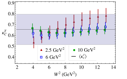
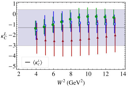
Figure 7: (color online) Continuum parameters $\kappa_{C}^{T}$ (left) and $\kappa_{C}^{L}$ (right) fitted to the DIS data, parametrized by the ABM11 global QCD fit Alekhin et al. (2012), as a function of $W^{2}$ for fixed $Q^{2}=2.5$ GeV² (red triangles), 6 GeV² (blue squares), and 10 GeV² (green circles). The average values $\langle\kappa_{C}^{T,L}\rangle$ are indicated by the solid lines, with the shaded band giving their uncertainty. Note that some of the points have been slightly offset for clarity.

The central values of $\kappa_{C}^{T,L}$ are computed by averaging over the three sets of $Q^{2}$ values, and the uncertainty determined by taking into account both the $W^{2}$ dependence of the fits and the PDF error. Because the $\kappa_{C}^{T,L}$ values at the different $Q^{2}$ are correlated, performing a simple $\chi^{2}$ fit to all the sets may underestimate the errors. As a more reliable error estimate, we combine in quadrature the uncertainties arising from (i) the $W^{2}$ dependence, for which we take the average of the difference between the central values of the lowest and highest points for the $Q^{2}$ set giving the strongest $W^{2}$ dependence (namely, for $Q^{2}=2.5$ GeV² for $\kappa_{C}^{T}$, and $Q^{2}=10$ GeV² for $\kappa_{C}^{L}$); and (ii) the PDF error, the uncertainty for which is given by the data point with the largest error in the entire set (which occurs for $Q^{2}=2.5$ GeV² for both $\kappa_{C}^{T}$ and $\kappa_{C}^{L}$). The final fitted values of the continuum parameters are found to be

$$\kappa_{C}^{T}=0.65\pm 0.14\,,\qquad\qquad\kappa_{C}^{L}=-1.3\pm 1.7\,.$$ (31)

Compared with the uncertainties assumed by GHRM Gorchtein et al. (2011) our uncertainty on the transverse parameter $\kappa_{C}^{T}$ is about five times smaller, while that on the longitudinal parameter $\kappa_{C}^{L}$ is almost two and a half times larger. However, the error on $\kappa_{C}^{L}$ has minimal effect on the $\gamma Z$ cross section at these kinematics because of the relatively small contribution of the longitudinal structure function.

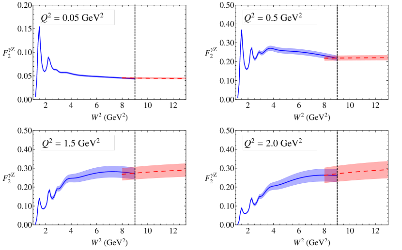
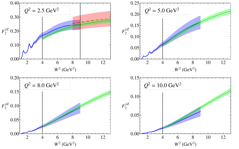
Figure 8: (color online) Proton $F_{2}^{\gamma Z}$ structure function versus $W^{2}$ at various fixed $Q^{2}$ values for the low-$W$ CB fit Christy and Bosted (2010) (blue solid) and the high-$W$ VMD+Regge Alwall and Ingelman (2004) (red dashed) and ABM11 Alekhin et al. (2012) (green dotted) parametrizations. The boundaries between the Regions I, II and III are indicated by the vertical lines at $W^{2}=4$ and 9 GeV².

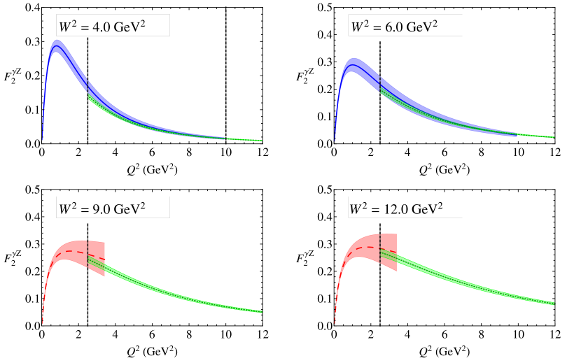
Figure 9: (color online) Proton $F_{2}^{\gamma Z}$ structure function versus $Q^{2}$ at fixed $W^{2}=4$, 6, 9 and 12 GeV² for the CB fit Christy and Bosted (2010) (blue solid), the ABM11 PDF parametrization Alekhin et al. (2012) (green dotted), and the VMD+Regge model Alwall and Ingelman (2004) (red dashed), with the boundaries between Regions I, II and III indicated by the vertical lines at fixed $Q^{2}$.

The resulting $F_{2}^{\gamma Z}$ structure function with the constrained $\kappa_{C}^{T,L}$ values is shown in Fig. 8 for fixed $Q^{2}$, ranging from $Q^{2}=0.05$ to 10 GeV². The models of the $\gamma Z$ structure functions are seen to match very well at the boundaries between the Regions I, II and III. As for the interference $F_{2}^{\gamma Z}$ structure function in Fig. 6, only the continuum uncertainty is included in these examples; this allows a direct comparison with the uncertainty in the GHRM model input which dominates all other uncertainties. The comparison between Figs. 6 and 8 at the corresponding kinematics illustrates the significant reduction in the $F_{2}^{\gamma Z}$ uncertainty that results from constraining the structure functions by the global QCD fits of PDFs. A similarly large reduction in the uncertainty can be seen in Fig. 9 for $F_{2}^{\gamma Z}$ as a function of $Q^{2}$ at fixed $W^{2}$ values.

The remaining uncertainty on the background contribution is associated with the $R_{\omega}^{T,L}$ and $R_{\phi}^{T,L}$ terms in Eq. (24). Following GHRM Gorchtein et al. (2011), we take the difference between these ratios calculated in the VMD+Regge model at $Q^{2}=7$ GeV² and the experimental vector meson cross sections from HERA Breitweg et al. (2000), assuming $R_{\omega}^{T}=R_{\omega}^{L}$ and $R_{\phi}^{T}=R_{\phi}^{L}$ (see Fig. 13 of Gorchtein et al. (2011)). This uncertainty is then added in quadrature with the continuum uncertainty, along with the resonance contribution discussed in Sec. III, to obtain the total error on the $\gamma Z$ structure functions used in estimating $\Re e\,\square_{\gamma Z}^{V}\$.

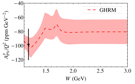
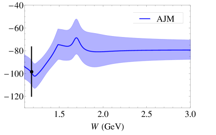
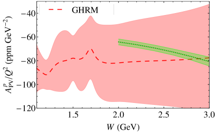
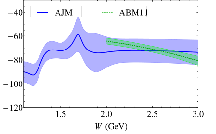
Figure 10: (color online) Proton parity-violating inelastic asymmetry $A_{\rm PV}/Q^{2}$ as a function of $W$, at fixed incident energy $E=0.69$ GeV and $Q^{2}=0.34$ GeV², for the GHRM Model II Gorchtein et al. (2011) (left) and the AJM model (right). The data point at $W=1.18$ GeV (black circle) is from the Jefferson Lab G0 experiment Androic et al. (2012).

Figure 11: (color online) Proton parity-violating inelastic asymmetry $A_{\rm PV}/Q^{2}$ as a function of $W$, at fixed incident energy $E=6$ GeV and $Q^{2}=2.5$ GeV², for the GHRM Model II Gorchtein et al. (2011) (left) and the AJM model (right). The asymmetry computed directly from PDFs Alekhin et al. (2012) is represented by the green band.

The impact of the total uncertainty reduction is illustrated in Figs. 11 and 11 for the parity-violating inelastic asymmetry for the proton,

$$A_{\rm PV} = g_{A}^{e}{\left(\frac{G_{F}Q^{2}}{2\sqrt{2}\pi\alpha}\right)\frac{xy^{2}F_{1}^{\gamma Z}+\left(1-y-\displaystyle{x^{2}y^{2}M^{2}\over Q^{2}}\right)F_{2}^{\gamma Z}+\displaystyle{g_{V}^{e}\over g_{A}^{e}}\left(y-\frac{1}{2}y^{2}\right)xF_{3}^{\gamma Z}}{xy^{2}F_{1}^{\gamma\gamma}+\left(1-y-\displaystyle{x^{2}y^{2}M^{2}\over Q^{2}}\right)F_{2}^{\gamma\gamma}}},$$ (32)

where $y=\nu/E$ is the fractional energy transferred to the target. In addition to the vector $F_{1,2}^{\gamma Z}$ structure functions, the asymmetry $A_{\rm PV}$ depends also on the axial-vector $F_{3}^{\gamma Z}$ structure function. For the the resonance contribution to $F_{3}^{\gamma Z}$ we use the parametrization of the axial-vector transition form factors of Lalakulich et al. Lalakulich and Paschos (2005); Lalakulich et al. (2006, 2007). For the background we follow Ref. Carlson and Rislow (2012) and rescale the electromagnetic cross sections Christy and Bosted (2010) by the average of the $x\to 0$ and SU(6) quark model limits, which gives $F_{3}^{\gamma Z}=5/3\,F_{1}^{\gamma\gamma}$. (Note that for the deuteron this average becomes $F_{3}^{\gamma Z}=9/5\,F_{1}^{\gamma\gamma}$.)

The asymmetries calculated in the AJM and GHRM models are shown in Fig. 11 at an incident energy $E=0.69$ GeV and $Q^{2}=0.34$ GeV², corresponding to the kinematics of the recent G0 measurement at Jefferson Lab near the $\Delta$ resonance region Androic et al. (2012). The central values of both models agree well with the data, although the experimental uncertainty is too large to enable meaningful constraints to be placed on the $\gamma Z$ structure functions. The constraint on the $\kappa_{C}^{T}$ value from matching to the DIS structure functions in the AJM model renders the uncertainty band somewhat smaller than the GHRM uncertainty Gorchtein et al. (2011) at higher values of $W$. (Note that the uncertainty on $A_{\rm PV}$ is computed by taking the upper and lower values of the input $\gamma Z$ structure functions, and is therefore asymmetric.)

The difference in the error bands becomes more pronounced at larger $Q^{2}$, as seen in Fig. 11 at $E=6$ GeV and $Q^{2}=2.5$ GeV², which are representative of typical kinematics at Jefferson Lab (see Sec. IV.2 below). Here the uncertainty on the GHRM model asymmetry at $W\sim 2$ GeV is around four times larger than the corresponding uncertainty on the constrained AJM model asymmetry. For comparison, we also show in Fig. 11 the asymmetry computed directly from PDFs Alekhin et al. (2012) in the region $W>2$ GeV where a partonic description is expected to be valid.

The uncertainty in the PDF-based calculation is slightly smaller than, but qualitatively similar to, that in the AJM model, while the GHRM model uncertainty is significantly overestimated in the region of overlap. We stress that although the DIS region makes only a modest contribution to $\Re e\,\square_{\gamma Z}^{V}\$, the requirement that the $\gamma Z$ cross sections match across the DIS-resonance region boundary imposes strong constraints on the $\gamma Z$ structure functions also at lower $W$ and $Q^{2}$. In the following section we confront this against new data on parity-violating electron-deuteron scattering in the resonance region.

IV.2 Deuteron asymmetry

The E08-011 experiment Zheng (2013); Wang et al. (2013) at Jefferson Lab recently measured the parity-violating asymmetry in inclusive electron-deuteron scattering over a range of $W$ and $Q^{2}$ in both the resonance and DIS regions. While the DIS region data are currently still being analyzed Zheng (2013), the available resonance region data Wang et al. (2013) can be used to provide an independent test of the procedure for estimating the $\gamma Z$ structure functions. This is particularly important for $\Re e\,\square_{\gamma Z}^{V}\$, since the integrals in Eq. (12) are dominated by Region I in Fig. 2.

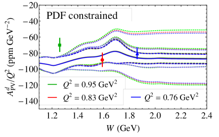
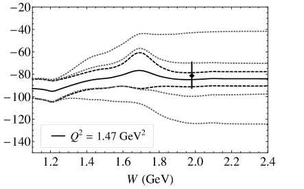
Figure 12: (color online) Deuteron parity-violating asymmetry $A_{\rm PV}^{d}/Q^{2}$ as a function of $W$ for incident electron energy $E=4.9$ GeV (left) and $E=6.1$ GeV (right). The data points from the Jefferson Lab E08-011 experiment Wang et al. (2013) at $W=1.26$ (green square), 1.59 (red circle), 1.86 (blue triangle) and 1.98 GeV (black diamond) correspond to average values of $Q^{2}=0.95$, 0.83, 0.76 and 1.47 GeV², respectively. The AJM model uncertainties (inner dashed band) are constrained by matching the continuum parameters $\kappa_{C}^{T,L}(d)$ to the DIS region $\gamma Z$ structure functions Alekhin et al. (2012), and are compared with those computed with errors on $\kappa_{C}^{T,L}(d)$ of 100% (outer dotted bands) and 25% (inner dotted bands).

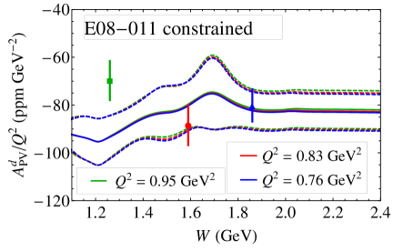
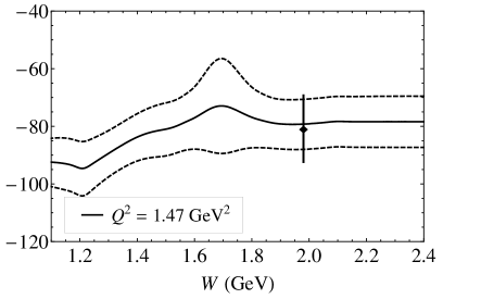
Figure 13: (color online) As in Fig. 12, but with the AJM model asymmetries (solid) and their uncertainties (dashed) constrained by the E08-011 data Wang et al. (2013). Note the different scale on the ordinate to that in Fig. 12.

The measured parity-violating asymmetry $A_{\rm PV}^{d}$, scaled by $1/Q^{2}$, is shown in Fig. 12 at $W=1.26$, 1.59, 1.86 and 1.98 GeV, with $Q^{2}$ values ranging from 0.76 to 1.47 GeV². (The $1/Q^{2}$ scaling factor enables the various points to be shown on the same graph.) The deuteron asymmetries in the AJM model are computed with the continuum parameters constrained by the DIS region structure functions computed from global PDFs Alekhin et al. (2012), as for the proton asymmetry in the previous section (see Fig. 11). The resulting fit gives for the transverse continuum parameter $\kappa_{C}^{T}(d)=0.79\pm 0.05$, and is in excellent agreement with the E08-011 data Wang et al. (2013) for all kinematics, except at the $\Delta$ region point at $Q^{2}=0.95$ GeV², where it lies slightly below the data. Since the calculation of the $\Delta$ resonance contribution to $A_{\rm PV}^{d}$ relies only on isospin symmetry and the conservation of the vector current, its uncertainty is smaller than that for higher-mass resonances. The discrepancy may reflect stronger isospin dependence of the nonresonant background for $\Delta$ production Mukhopadhyay et al. (1998), although the difference is at the $\lesssim 2\sigma$ level. Also, as seen in Fig. 11 above, the models agree well with the G0 data Androic et al. (2012) in the $\Delta$ region, albeit within larger errors.

By using the longitudinal structure function from the global QCD fit in Ref. Alekhin et al. (2012), we find for the longitudinal continuum parameter $\kappa_{C}^{L}(d)=0.2\pm 3.4$. Although the specific implementation of the CB parametrization Christy and Bosted (2010) prevents this uncertainty from being propagated directly into $A_{\rm PV}^{d}$, we nevertheless can use the $\kappa_{C}^{T,L}$ values for the proton to ensure that the uncertainty in the longitudinal piece is taken into account. For comparison, we also show in Fig. 12 the uncertainty that would be obtained with a similar 100% error on the continuum parameters as was assumed by GHRM for the proton, with the VMD+Regge model Alwall and Ingelman (2004) used for the entire kinematic region Gorchtein et al. (2011). In this case the uncertainties on $A_{\rm PV}^{d}$ in the $W\gtrsim 1.8$ GeV region are $\approx 6$ times larger than the AJM model asymmetries. Using a reduced 25% uncertainty on $\kappa_{C}^{T}(d)$ results in asymmetries with a significantly smaller error band, which is nevertheless slightly larger than in the AJM model.

As a check, the parameter $\kappa_{C}^{T}(d)$ was also constrained by performing a $\chi^{2}$ fit to the E08-011 data points. This fit constrains the dominant, transverse continuum parameter to be $\kappa_{C}^{T}(d)=0.69\pm 0.13$. [Omitting the $\Delta$ datum from the fit would yield a marginally larger value, $\kappa_{C}^{T}(d)=0.72\pm 0.13$.] For the longitudinal contribution, the CB parametrization of the deuteron structure function provides only $F_{1}^{\gamma\gamma}$, while $F_{L}^{\gamma\gamma}$ is obtained through the longitudinal to transverse cross section ratio $\sigma_{L}^{\gamma\gamma}/\sigma_{T}^{\gamma\gamma}$ [see Eq. (21)], with the deuteron ratio assumed to be the same as for the proton. Within this parametrization, a direct constraint on $\kappa_{C}^{L}(d)$ as for the proton case is therefore not possible. However, as for the PDF-constrained asymmetry, we can still propagate the uncertainty on $\sigma_{L}/\sigma_{T}$ through the final asymmetry by including the uncertainties in the $\kappa_{C}^{T,L}$ values of the proton which serve as inputs into the $\sigma_{L}^{\gamma Z}/\sigma_{T}^{\gamma Z}$ ratio.

Table 2: Parity-violating deuteron asymmetries in the AJM model at the kinematics of the E08-011 experiment Zheng (2013); Wang et al. (2013). The asymmetries are computed with the continuum parameters $\kappa_{C}^{T,L}(d)$ constrained by the E08-011 data, or by matching to the DIS region described in terms of PDFs. Note that the points marked with asterisks (^∗) are predictions.

$E$	$W$	$Q^{2}$	$A_{\rm PV}/Q^{2}$ (ppm GeV-2)
(GeV)	(GeV)	(GeV2)	PDF constraint	E08-011 constraint
4.9	1.26	0.95	$-93.7_{-9.0}^{+8.8}$	$-93.1_{-9.0}^{+8.8}$
4.9	1.59	0.83	$-82.7_{-9.9}^{+9.7}$	$-80.1_{-10.3}^{+10.1}$
4.9	1.86	0.76	$-86.2_{-6.9}^{+6.7}$	$-82.4_{-8.0}^{+7.9}$
6.1	1.98	1.47	$-84.7_{-6.4}^{+6.2}$	$-79.2_{-8.8}^{+8.6}$
6.1	2.03	1.28	$-84.9_{-6.4}^{+6.2}$${}^{\ (*)}$	$-79.7_{-8.6}^{+8.4}$${}^{\ (*)}$
6.1	2.07	1.09	$-85.2_{-6.4}^{+6.2}$${}^{\ (*)}$	$-80.3_{-8.3}^{+8.2}$${}^{\ (*)}$
6.1	2.33	1.90	$-82.7_{-6.5}^{+6.3}$${}^{\ (*)}$	$-76.5_{-9.3}^{+9.3}$${}^{\ (*)}$

The resulting asymmetries are again in very good agreement with the E08-011 data, as is seen in Fig. 13. Moreover, the uncertainties (dashed curves) are three to four times smaller in the $W\gtrsim 1.8$ GeV region than those obtained by assuming a 100% uncertainty on the parameters, and remain smaller than even for the reduced, 25% uncertainty case. The consistency between the data and the results given by the constrained expressions gives us confidence in the reliability of the $\gamma Z$ structure functions in the AJM model in the region of low to intermediate $W$ and $Q^{2}$ that is of greatest importance for the $\Re e\,\square_{\gamma Z}^{V}\$calculation.

Finally, the values of the calculated asymmetries and their uncertainties, using both the resonance region data and the PDF constraints, are summarized in Table 2 at each of the kinematic points from the E08-011 experiment Wang et al. (2013). In addition, we list the AJM model predictions for $A_{\rm PV}^{d}$ at the measured DIS region points at $W>2$ GeV (marked by asterisks), which will be discussed further in the next section.

V Results

V.1 $\gamma Z$ box corrections for $Q_{\text{weak}}\,\,$

The detailed examination of the $\gamma Z$ interference structure functions and their uncertainties, constrained by data in the DIS region and parity-violating asymmetries in the resonance region, allows us to compute the $\Im m\,\square_{\gamma Z}^{V}\$correction in Eq. (12), and through the dispersion relation (6) to make a reliable determination of the $\gamma Z$ box correction to $Q_{W}^{p}$. The dependence of $\Re e\,\square_{\gamma Z}^{V}\$on the incident energy $E$ is illustrated in Fig. 14, which also shows the individual contributions of the various $W$ and $Q^{2}$ regions in Fig. 2.

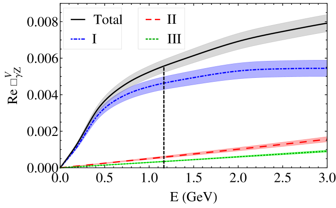
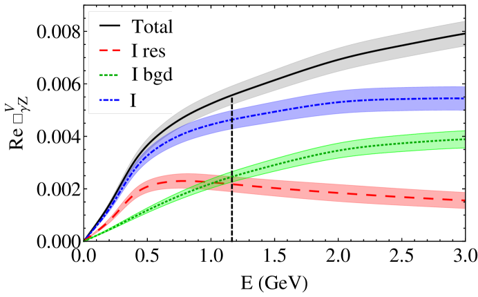
Figure 14: (color online) Energy dependence of the contributions to $\Re e\,\square_{\gamma Z}^{V}\$from the various regions in $W$ and $Q^{2}$ displayed in Fig. 2 in the AJM model (top), and the breakdown of Region I into its resonant and nonresonant background components (bottom).

At low energy ($E\lesssim 1$ GeV), the total correction $\Re e\,\square_{\gamma Z}^{V}\$is dominated by the low-$W$, low-$Q^{2}$ region (Region I in Fig. 2). As found in earlier analyses Gorchtein and Horowitz (2009); Tjon et al. (2009); Sibirtsev et al. (2010); Rislow and Carlson (2011); Gorchtein et al. (2011), the resonant contribution [mainly from the $\Delta(1232)$ resonance] peaks at around $E\approx 0.7$ GeV, and gradually decreases at higher energies. The nonresonant and resonant components of Region I are approximately equal at $E\sim 1$ GeV, with the nonresonant part growing with increasing energy. The higher-$W$, higher-$Q^{2}$ regions play a relatively minor role in the $\square_{\gamma Z}^{V}\,$correction, with Regions II and III contributing $\approx 20\%$ and 10% of the total, at $E=3$ GeV, respectively.

Table 3: Contributions to $\Re e\,\square_{\gamma Z}^{V}\$from various regions in $W$ and $Q^{2}$ in the AJM model (see Fig. 2) at the $Q_{\text{weak}}\,\,$energy $E=1.165$ GeV.

Region	$\Re e\,\square_{\gamma Z}^{V}\$ ($\times 10^{-3}$)
I (res)	$2.18\pm 0.29$
I (bgd)	$2.46\pm 0.20$
I (total)	$4.64\pm 0.35$
II	$0.59\pm 0.05$
III	$0.35\pm 0.02$
Total	$5.57\pm 0.36$

At the $Q_{\text{weak}}\,\,$energy, $E=1.165$ GeV, the breakdown of the $\Re e\,\square_{\gamma Z}^{V}\$correction into its individual contributions is summarized in Table 3. Including uncertainties from all regions, the total correction is found to be

$$\Re e\,\square_{\gamma Z}^{V}=(5.57\pm 0.21_{\,\rm[bgd]}\pm 0.29_{\,\rm[res]}\pm 0.02_{\,\rm[DIS]})\times 10^{-3},$$ (33)

where the uncertainties listed are from the nonresonant background, the resonances, and the DIS region, respectively. Adding the errors in quadrature gives $\Re e\,\square_{\gamma Z}^{V}=(5.57\pm 0.36)\times 10^{-3}$ at the $Q_{\text{weak}}\,\,$energy. The $\approx 7\%$ relative uncertainty on this correction remains largely energy independent, even at large energies, where the contributions from larger $W$ and $Q^{2}$ become more important; since the structure functions are constrained by DIS data, the uncertainty in $\Re e\,\square_{\gamma Z}^{V}\$does not grow with $E$.

The AJM model value of the $\gamma Z$ box correction is similar to the result, $\Re e\,\square_{\gamma Z}^{V}=(5.40\pm 0.54)\times 10^{-3}$, obtained using the $\gamma Z$ structure functions from Region II extended over all kinematics, as in the GHRM Model II Gorchtein et al. (2011), but with the $\kappa_{C}^{T,L}$ parameters constrained by matching to the DIS region structure functions Alekhin et al. (2012). This constraint renders the uncertainty $\sim$ four times smaller than that in Ref. Gorchtein et al. (2011), but still slightly larger than in the AJM model calculation.

V.2 Predictions for parity-violating asymmetries

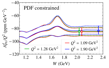
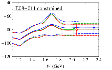
Figure 15: (color online) Predictions for the parity-violating deuteron asymmetry $A_{\rm PV}^{d}/Q^{2}$ as a function of $W$ (solid) for the DIS region kinematics of the Jefferson Lab E08-011 experiment Zheng (2013) at $Q^{2}=1.28$ GeV² (green), 1.09 GeV² (red) and 1.90 GeV² (blue) (see also Table 2). The uncertainties (dashed) are computed in the AJM model with the continuum parameters $\kappa_{C}^{T,L}$ constrained by DIS structure functions (left), and by the E08-011 resonance region data (right). The predictions at the experimental $W$ values Zheng (2013) are shown as pseudo-data points (open symbols).

The $\gamma Z$ structure functions can be further constrained by additional parity-violating asymmetry data from the E08-011 experiment at Jefferson Lab Zheng (2013); Wang et al. (2013). The deep-inelastic region data are currently being analyzed Zheng (2013), and the predictions from the AJM model are shown in Fig. 15 as a function of $W$ for the three experimental $Q^{2}$ values (see also Table 2). The uncertainties on the predictions are computed both by fitting the continuum parameters $\kappa_{C}^{T,L}$ to the DIS structure functions Alekhin et al. (2012) and the E08-011 resonance region data Wang et al. (2013). The asymmetries with the E08-011 data constraints are marginally higher than those with the parameters constrained by PDFs, with slightly larger uncertainties. As for the resonance region comparison in Figs. 12 and 13, these uncertainties are $\approx$ four to five times smaller than they would be without the constraints on $\kappa_{C}^{T,L}$, assuming 100% errors along the lines of the proton calculation in Ref. Gorchtein et al. (2011). The upcoming data will therefore be extremely useful in determining the uncertainties on the $\gamma Z$ structure functions and on the resulting $\Re e\,\square_{\gamma Z}^{V}\$correction.

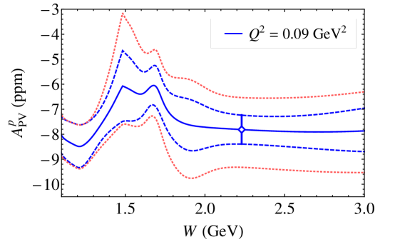
Figure 16: (color online) AJM model prediction for the proton parity-violating asymmetry $A_{\rm PV}^{p}$ as a function of $W$ for the $Q_{\text{weak}}\,\,$inelastic measurement Carlini (2012) at $Q^{2}=0.09$ GeV² (solid line and open symbol). The AJM model uncertainties (dashed) are compared with those from the GHRM model with 100% uncertainty on the continuum parameters (dotted).

A further constraint will be provided by the inelastic $Q_{\text{weak}}\,\,$measurement Carlini (2012), which was a special run of the $Q_{\text{weak}}\,\,$experiment tuned to the inelastic region at an average $W=2.23$ GeV. The AJM model prediction for the proton asymmetry $A_{\rm PV}^{p}$ and its uncertainty are shown in Fig. 16, where we find $A_{\rm PV}^{p}=(-7.8\pm 0.6)$ ppm at the experimental $Q^{2}=0.09$ GeV² value. The uncertainty in the AJM model, with the continuum parameters $\kappa_{C}^{T,L}$ constrained by the DIS structure functions, is $\approx$ two times smaller at the inelastic $Q_{\text{weak}}\,\,$kinematic point than that from the GHRM model Gorchtein et al. (2011) without these constraints. Note also that in the resonance region, $W\sim 1.5$ GeV, the uncertainty in the GHRM model almost doubles by taking extrema values instead of the more conventional addition in quadrature. The inelastic $Q_{\text{weak}}$, and similar measurements of the parity-violating inelastic asymmetries, will be valuable for constraining the $\gamma Z$ structure functions and the $\Re e\,\square_{\gamma Z}^{V}\$corrections in the future.

VI Conclusion

We have performed a comprehensive analysis of the $\gamma Z$ box contribution to the forward electron-proton elastic parity-violating asymmetry. Our primary result is a new determination of the uncertainty on $\Re e\,\square_{\gamma Z}^{V}\$ at the beam energy of the $Q_{\text{weak}}\,\,$experiment. In comparison with previous estimates, we report a significant reduction in this uncertainty, driven largely by data on structure functions in the DIS region, and measurements of parity-violating asymmetries in the resonance region.

To isolate the dependence on the various inputs required in the evaluation of $\Re e\,\square_{\gamma Z}^{V}\$, we have divided the dispersion integral into three kinematic regions. Region I, which includes resonance contributions at low $W$ and $Q^{2}$, is identified to totally dominate the value of $\Re e\,\square_{\gamma Z}^{V}\$. The total uncertainty is therefore largely driven by how well the $\gamma Z$ interference structure functions $F_{i}^{\gamma Z}$ can be constrained in this region.

The resonance region $\gamma Z$ structure functions are determined by an isospin transformation of the corresponding $\gamma\gamma$ structure functions. The input $F_{i}^{\gamma\gamma}$ functions are determined by a fit Christy and Bosted (2010) to the world’s inclusive electron-nucleon scattering data in terms of resonance contributions and a nonresonant background. For the resonance components, the isospin transformation can be performed using the conservation of the vector current and the isospin dependence of the couplings, as reported by the PDG, with relatively modest contribution to the overall uncertainty. For the background, following the approach of Ref. Gorchtein et al. (2011), the transformation is estimated using a prescription based on the VMD model Alwall and Ingelman (2004). For the low-mass vector meson components the isospin rotation is determined by isospin symmetry of the electroweak interactions, while the transformation of the high-mass continuum part is not fixed within the VMD formalism, and consequently contributes a larger uncertainty.

At larger $Q^{2}$ values ($Q^{2}>1.5$ GeV²) the continuum piece totally dominates the nonresonant background. We use this fact to constrain the continuum component of the isospin rotation by matching this to the DIS structure functions in the transition region. The model dependence from using a particular continuum form at lower $Q^{2}$ (away from the PDF constraint) is less important, since this region is dominated by the low-mass vector mesons $\rho$, $\omega$ and $\phi$. It is the constraint on this rotation that drives the significant reduction in uncertainty in the present AJM model as compared to that reported by GHRM Gorchtein et al. (2011).

Combined with the relatively well-determined contributions from Regions II and III at higher $W$ and $Q^{2}$ (see Fig. 2), we find the final value for $\gamma Z$ correction to be $\Re e\,\square_{\gamma Z}^{V}\$$=(5.57\pm 0.36)\times 10^{-3}$. Importantly, this precision maintains confidence in the interpretation of the $Q_{\text{weak}}\,\,$experiment as a standard model test.

The reliability of our constraint procedure has been confirmed by a comparison with the corresponding inclusive $\gamma Z$ interference asymmetries recently measured on the deuteron by the E08-011 experiment at Jefferson Lab Wang et al. (2013). Conversely, using the E08-011 resonance region data as a constraint on the $\gamma Z$ structure functions, the resulting asymmetries are found to be very similar to those in the AJM model with the PDF constraints, albeit with slightly larger uncertainties. Upcoming data on the deuteron asymmetry in the DIS region Zheng (2013) should reduce these uncertainties.

Beyond this, the most promising means by which one could further constrain the $\gamma Z$ structure functions would be to perform a systematic experimental study of parity-violating electron scattering on hydrogen across Region I. While the recent deuterium measurements Wang et al. (2013) have proven useful in providing confidence in the procedure of matching to PDFs at intermediate $Q^{2}$ and $W$, because the deuteron requires a knowledge of the neutron structure function as well as of the proton, this has limited value as a means to reduce the uncertainty in $F_{i}^{\gamma Z}$. A dedicated study of the proton itself would directly constrain the model and lead to a reduction in the uncertainty of the radiative correction arising from the $\gamma Z$ box.

References

- Sirlin and Ferroglia (2013) A. Sirlin and A. Ferroglia, Rev. Mod. Phys. 85, 263 (2013).
- (2) K. S. Kumar, S. Mantry, W. J. Marciano, and P. A. Souder, eprint arXiv:1302.6263 [Annu. Rev. Nucl. Part. Sci. (to be published)].
- Erler and Su (2013) J. Erler and S. Su, Prog. Part. Nucl. Phys. 71, 119 (2013).
- Armstrong et al. (2012) D. S. Armstrong et al., eprint arXiv:1202.1255.
- Musolf et al. (1994) M. J. Musolf, T. W. Donnelly, J. Dubach, S. J. Pollock, S. Kowalski, and E. J. Beise, Phys. Rep. 239, 1 (1994).
- Erler et al. (2003) J. Erler, A. Kurylov, and M. J. Ramsey-Musolf, Phys. Rev. D 68, 016006 (2003).
- Marciano and Sirlin (1983) W. J. Marciano and A. Sirlin, Phys. Rev. D 27, 552 (1983).
- Marciano and Sirlin (1984) W. J. Marciano and A. Sirlin, Phys. Rev. D 29, 75 (1984).
- Musolf and Holstein (1990) M. J. Musolf and B. R. Holstein, Phys. Lett. B 242, 461 (1990).
- Arrington et al. (2011) J. Arrington, P. G. Blunden, and W. Melnitchouk, Prog. Part. Nucl. Phys. 66, 782 (2011).
- Gorchtein and Horowitz (2009) M. Gorchtein and C. J. Horowitz, Phys. Rev. Lett. 102, 091806 (2009).
- Sibirtsev et al. (2010) A. Sibirtsev, P. G. Blunden, W. Melnitchouk, and A. W. Thomas, Phys. Rev. D 82, 013011 (2010).
- Rislow and Carlson (2011) B. C. Rislow and C. E. Carlson, Phys. Rev. D 83, 113007 (2011).
- Gorchtein et al. (2011) M. Gorchtein, C. J. Horowitz, and M. J. Ramsey-Musolf, Phys. Rev. C 84, 015502 (2011).
- Wang et al. (2013) D. Wang et al., eprint arXiv:1304.7741.
- Carlini (2012) R. Carlini (private communication).
- Wood et al. (1997) C. S. Wood, S. C. Bennett, D. Cho, B. P. Masterson, J. L. Roberts, C. E. Tanner, and C. E. Wieman, Science 275, 1759 (1997).
- Dzuba and Flambaum (2012) V. A. Dzuba and V. V. Flambaum, Int. J. Mod. Phys. E21, 1230010 (2012).
- Blunden et al. (2011) P. G. Blunden, W. Melnitchouk, and A. W. Thomas, Phys. Rev. Lett. 107, 081801 (2011).
- Blunden et al. (2012) P. G. Blunden, W. Melnitchouk, and A. W. Thomas, Phys. Rev. Lett. 109, 262301 (2012).
- Zhou et al. (2007) H. Q. Zhou, C. W. Kao, and S. N. Yang, Phys. Rev. Lett. 99, 262001 (2007).
- Tjon et al. (2009) J. A. Tjon, P. G. Blunden, and W. Melnitchouk, Phys. Rev. C 79, 055201 (2009).
- Aaron et al. (2012) F. D. Aaron et al. (H1 Collaboration), J. High Energy Phys. 09 (2012) 061.
- Christy and Bosted (2010) M. E. Christy and P. E. Bosted, Phys. Rev. C 81, 055213 (2010).
- Bosted and Christy (2008) P. E. Bosted and M. E. Christy, Phys. Rev. C 77, 065206 (2008).
- Cvetic et al. (2001) G. Cvetic, D. Schildknecht, B. Surrow, and M. Tentyukov, Eur. Phys. J. C 20, 77 (2001).
- Cvetic et al. (2000) G. Cvetic, D. Schildknecht, and A. Shoshi, Eur. Phys. J. C 13, 301 (2000).
- Sakurai and Schildknecht (1972) J. J. Sakurai and D. Schildknecht, Phys. Lett. B 40, 121 (1972).
- Alwall and Ingelman (2004) J. Alwall and G. Ingelman, Phys. Lett. B 596, 77 (2004).
- Capella et al. (1994) A. Capella, A. Kaidalov, C. Merino, and J. Tran Thanh Van, Phys. Lett. B 337, 358 (1994).
- Carlson and Rislow (2012) C. E. Carlson and B. C. Rislow, Phys. Rev. D 85, 073002 (2012).
- Nakamura et al. (2010) K. Nakamura et al. (Particle Data Group), J. Phys. G 37, 075021 (2010).
- Tiator et al. (2011) L. Tiator, D. Drechsel, S. S. Kamalov, and M. Vanderhaeghen, Eur. Phys. J. ST 198, 141 (2011).
- Kuroda and Schildknecht (2012) M. Kuroda and D. Schildknecht, Phys. Rev. D 85, 094001 (2012).
- Fraas et al. (1975) H. Fraas, B. J. Read, and D. Schildknecht, Nucl. Phys. B86, 346 (1975).
- Bauer et al. (1978) T. H. Bauer, R. D. Spital, D. R. Yennie, and F. M. Pipkin, Rev. Mod. Phys. 50, 261 (1978).
- Donnachie and Landshoff (1992) A. Donnachie and P. V. Landshoff, Phys. Lett. B 296, 227 (1992).
- Lai et al. (2010) H.-L. Lai, M. Guzzi, J. Huston, Z. Li, P. M. Nadolsky, J. Pumplin, and C.-P. Yuan, Phys. Rev. D 82, 074024 (2010).
- Martin et al. (2003) A. D. Martin, R. G. Roberts, W. J. Stirling, and R. S. Thorne, Eur. Phys. J. C 28, 455 (2003).
- Alekhin et al. (2012) S. Alekhin, J. Blumlein, and S. Moch, Phys. Rev. D 86, 054009 (2012).
- Accardi et al. (2011) A. Accardi, W. Melnitchouk, J. F. Owens, M. E. Christy, C. E. Keppel, L. Zhu, and J. G. Morfín, Phys. Rev. D 84, 014008 (2011).
- Owens et al. (2012) J. F. Owens, A. Accardi, and W. Melnitchouk, Phys. Rev. D 87, 094012 (2013).
- Ball et al. (2010) R. D. Ball, L. D. Debbio, S. Forte, A. Guffanti, J. I. Latorre, J. Rojo, and M. Ubiali, Nucl. Phys. B838, 136 (2010).
- Jimenez-Delgado and Reya (2009) P. Jimenez-Delgado and E. Reya, Phys. Rev. D 80, 114011 (2009).
- Martin et al. (2009) A. D. Martin, W. J. Stirling, R. S. Thorne, and G. Watt, Eur. Phys. J. C 63, 189 (2009).
- Gorchtein (2012) M. Gorchtein (private communication).
- Beringer et al. (2012) J. Beringer et al. (Particle Data Group), Phys. Rev. D 86, 010001 (2012).
- Alekhin (2012) S. Alekhin (private communication).
- Breitweg et al. (2000) J. Breitweg et al., Phys. Lett. B 487, 273 (2000).
- Lalakulich and Paschos (2005) O. Lalakulich and E. A. Paschos, Phys. Rev. D 71, 074003 (2005).
- Lalakulich et al. (2006) O. Lalakulich, E. A. Paschos, and G. Piranishvili, Phys. Rev. D 74, 014009 (2006).
- Lalakulich et al. (2007) O. Lalakulich, W. Melnitchouk, and E. A. Paschos, Phys. Rev. C 75, 015202 (2007).
- Androic et al. (2012) D. Androic et al. (G0 Collaboration), eprint arXiv:1212.1637.
- Zheng (2013) X. Zheng (private communication).
- Mukhopadhyay et al. (1998) N. C. Mukhopadhyay, M. J. Ramsey-Musolf, J. Pollock, S. J. Liu, and H.-W. Hammer, Nucl. Phys. A633, 481 (1998).