The Coyote Universe Extended: Precision Emulation of the Matter Power Spectrum

Abstract

Modern sky surveys are returning precision measurements of cosmological statistics such as weak lensing shear correlations, the distribution of galaxies, and cluster abundance. To fully exploit these observations, theorists must provide predictions that are at least as accurate as the measurements, as well as robust estimates of systematic errors that are inherent to the modeling process. In the nonlinear regime of structure formation, this challenge can only be overcome by developing a large-scale, multi-physics simulation capability covering a range of cosmological models and astrophysical processes. As a first step to achieving this goal, we have recently developed a prediction scheme for the matter power spectrum (a so-called emulator), accurate at the 1% level out to $k\sim 1~{}$Mpc^-1 and $z=1$ for $w$CDM cosmologies based on a set of high-accuracy N-body simulations. It is highly desirable to increase the range in both redshift and wavenumber and to extend the reach in cosmological parameter space. To make progress in this direction, while minimizing computational cost, we present a strategy that maximally re-uses the original simulations. We demonstrate improvement over the original spatial dynamic range by an order of magnitude, reaching $k\sim 10~{}h$Mpc^-1, a four-fold increase in redshift coverage, to $z=4$, and now include the Hubble parameter as a new independent variable. To further the range in $k$ and $z$, a new set of nested simulations run at modest cost is added to the original set. The extension in $h$ is performed by including perturbation theory results within a multi-scale procedure for building the emulator. This economical methodology still gives excellent error control, $\sim 5\%$ near the edges of the domain of applicability of the emulator. A public domain code for the new emulator is released as part of the work presented in this paper.

1 Introduction

1.1 Background

The discovery of the accelerated expansion of the Universe by Riess et al. (1998) and Perlmutter et al. (1999), now confirmed by multiple observations, has had a tremendous impact on the field of observational and theoretical cosmology. Due to our near-complete ignorance regarding the origin of cosmic acceleration, the initial task is to better characterize the nature of the underlying cause, first by observational means. The primary focus in this endeavor is to decide whether the acceleration is caused by some form of dark energy, a cosmological constant being the simplest realization of this idea, or by some modification of general relativity on large cosmological scales.

Unfortunately, carrying out controlled experiments in cosmology is impossible – therefore, information relevant to the above task must be obtained by combining inferences from different kinds of observations. These observations include the measurement of the temperature anisotropy of the cosmic microwave background (CMB), the luminosity distance relation from supernova observations, and large scale structure probes, such as baryon acoustic oscillations (BAO), weak lensing, clustering of galaxies, and the abundance of galaxy clusters. Despite the impressive power of the observations, all cosmological probes are plagued with a large number of sources of systematic error. These can be broken up into two kinds, (i) those related to the observational techniques – shape measurements in weak lensing and the determination of cluster masses being two prominent examples, and (ii) those related to the uncertainties in the theoretical predictions and the (related) errors in solving cosmological statistical inverse problems. An important member of this latter class is the prediction accuracy of the matter power spectrum, the central theme of this paper.

Because robust results in cosmology must rely on combining a number of observational probes, each possessing their individual strengths and weaknesses (not all of which can be fully predicted in advance), the current strategy is to proceed with several survey missions. In the spectroscopic realm, ongoing or recently completed surveys focusing on the measurement of BAO and galaxy clustering include the Sloan Digital Sky Survey (SDSS) (Zehavi et al., 2011), the WiggleZ survey (Drinkwater et al., 2010) and the Baryon Oscillation Spectroscopic Survey (BOSS) (Schlegel, White, & Eisenstein, 2009) component of SDSS-III; planned next-generation missions include the Mid-Scale Dark Energy Spectroscopic Instrument (MS-DESI) and SuMIRe. Imaging surveys include SDSS, the Canada-France-Hawaii Telescope Legacy Survey (CFHTLS), the Kilo Degree Survey (KiDS) (de Jong et al. 2013), the recently started Dark Energy Survey (DES), and in the future, Subaru Measurement of Images and Redshifts (SuMIRe) (Sugai, 2012), the Large Synoptic Survey Telescope (LSST) (Abell et al., 2009), and Euclid (Refregier et al., 2010). The most recent constraints from weak lensing have been obtained by the CFHTLenS team (Kilbinger et al., 2012), analysis of SDSS data (Huff et al. 2011, Lin et al. 2011), and the Deep Lens Survey (DLS) (Jee et al. 2013). In the x-ray the next planned mission is eROSITA (Merloni et al., 2012), which will provide a significant update to results from prior surveys, such as the 400d cluster survey (Vikhlinin et al., 2009). In the CMB, high-resolution measurements by the Atacama Cosmology telescope (ACT) (Das et al., 2012) and the South Pole Telescope (SPT) (van Engelen et al., 2012) have confirmed the sensitivity of the CMB to the large scale distribution of matter (CMB lensing). Significantly, first results from the Planck mission have been recently released (Ade et al., 2013). For a comprehensive review of the current state-of-the-art (pre-Planck) we refer the reader to Weinberg et al. (2012).

With the advent of ambitious large-scale observational programs, emphasis on statistical errors will no longer be the sole driving force. The understanding, control, and reduction of systematic errors is the next major challenge – there are several cases where measurements are already systematics-limited. Additionally, in the nonlinear regime of structure formation, state of the art measurements are pushing up against the limits of available prediction accuracy from theoretical computations and associated modeling. Major simulation campaigns, in concert with observational inputs, will be needed to control the error budgets. The simulation-based theoretical modeling process – consisting of a combination of first-principles calculations and parameterized models – will have to account accurately, and robustly, for the nonlinear evolution of structure formation, gas physics, and complex feedback effects.

Two examples will suffice to provide illustrations of the sort of difficulties that have to be faced. The first is cluster cosmology – it was recently shown by Cunha & Evrard (2010) and Wu, Zentner, & Wechsler (2010) that the halo mass function has to be predicted at the 1% level of accuracy for a DES-like survey in order to avoid errors on dark energy parameters. At the same time, an error in the prediction of halo masses at the 2% level will translate into mass function uncertainties in the cluster mass range of 5-10% (Cf. Bhattacharya et al. 2011). The effect is particularly strong because of the exponential fall-off of the mass function at high masses. The second example relates to prediction error requirements for weak lensing shear. These are also severe – for the matter power spectrum, predictions at the percent level accuracy at $k\sim 10~{}h^{-1}$Mpc are needed to extract all available information on dark energy (Huterer & Takada, 2005). A more recent study by Hearin & Zentner (2011) concludes that the accuracy requirements are even more stringent – for imaging surveys such as LSST and Euclid, the power spectrum needs to be predicted at 0.5% accuracy out to $k\sim 5~{}h^{-1}$Mpc.

1.2 Fitting Functions vs. Emulators

Currently, it is common practice to use fitting functions motivated by theoretical heuristics and matched to simulations to provide the required modeling input. For instance, analyses of weak lensing measurements employ fitting functions for the matter power spectrum. Semboloni et al. (2006) used the Peacock and Dodds fitting function (Peacock & Dodds, 1996) as well as Halofit (Smith et al., 2003) for their analysis of the CFHTLS cosmic shear measurements. Lin et al. (2011) used Halofit for their recent SDSS analysis, as do Kilbinger et al. (2012) in the most recent CFHTLens analysis (they point out that an emulator would be more accurate but one was not available over the required redshift range) and Jee et al. (2013) for the DLS analysis. Over a limited $k$ range, the fitting functions are accurate at the $\sim 5-10\%$ level for $\Lambda$CDM models (see, e.g., Heitmann et al. 2010). The latest improvement of Halofit is provided by Takahashi et al. 2012; a comparison of our results with theirs is provided in Section 6.3.

For next-generation applications, the fitting function approach suffers from two deficiencies, first, error-control is non-uniform over cosmological model parameter space, and, second, the fitting process degrades the actual accuracy of the simulations used to build the parameterized fit. Moreover, because the fitting forms become essentially arbitrary as the accuracy requirements become more stringent, this strategy is difficult – if not impossible – to implement systematically across a large number of freely floating cosmological and modeling parameters.

Cluster mass functions provide another example of these difficulties – obtaining dark energy constraints from the abundance of clusters of galaxies as carried out in, e.g., Vikhlinin et al. (2009), employs fitting forms for the mass function; to extend these fits across cosmological models, the assumption of universality (Jenkins et al., 2001) is required. However, as shown in, e.g., Bhattacharya et al. (2011), universality for $w$CDM models only holds at the $\sim 10$% level of accuracy. It appears quite unlikely that a simple mass function fit – valid for a large class of dark energy models, covering a wide redshift range, and satisfying percent level accuracy requirements – will ever be attainable.

We have recently developed the “Cosmic Calibration Framework” (CCF) to provide accurate prediction schemes for cosmological observables (Heitmann et al. 2006, Habib et al. 2007) seeking to avoid the shortcomings of the fitting function approach mentioned above. The CCF contains error-controlled direct numerical oracles for the predicted quantities, as opposed to (potentially uncontrolled) analytic fitting forms. It aims to make tools available that provide essentially instantaneous predictions of large scale structure observables, e.g., the nonlinear power spectrum, mass functions for different halo definitions, or the halo concentration-mass relation.

At the heart of the CCF lies a sophisticated sampling scheme for optimally placing a given finite number of cosmological models in parameter space. Simulations are carried out at these parameter values (we use orthogonal-array Latin hybercubes as well as symmetric Latin hybercube designs). The next step is an efficient representation that translates the measurements from the simulations into functions that are conveniently interpolated (we use a principal component basis to provide a reduced data representation), and finally an accurate interpolation scheme over the basis functions (our choice here is Gaussian process modeling). For an introduction to the general framework, see, e.g., Santner et al. 2003.

The CCF was first described in Heitmann et al. (2006), with details and examples given in Habib et al. (2007). In a series of three papers (Coyote Universe I-III), we described the development of a precision emulator for the matter power spectrum over a five-dimensional parameter space ($\theta=\{\omega_{b},\omega_{m},n_{s},w,\sigma_{8}\}$). This emulator provides predictions for the power spectrum for $w$CDM cosmologies out to $k\sim 1$ Mpc^-1 at the 1% accuracy level for a redshift range of $0\leq z\leq 1$, over a relatively wide range of cosmological parameters (see Section 3). Since then, similar approaches have been followed in Schneider, Holm, & Knox (2011) and Agarwal et al. (2012) with some differences in the sampling and interpolation schemes used to build power spectrum emulators.

The CCF framework was extended in Schneider et al. (2008) to derive an approximate statistical model for the sample variance distribution of the nonlinear matter power spectrum. Eifler (2011) used the emulator to generate a weak-lensing prediction code to calculate various second-order cosmic shear statistics, e.g., shear power spectrum, shear-shear correlation function, ring statistics and Complete Orthogonal Set of EB-mode Integrals (COSEBIs). The emulator we presented in Lawrence et al. (2010) was used by Huff et al. (2011) in their analysis of SDSS weak lensing (where it was combined with Halofit to obtain the power spectrum at larger $k$ values). More CCF-based emulators are under development; a recent example is an emulator for the halo concentration-mass relation (Kwan et al., 2013).

Observational requirements, such as those for DES weak lensing, and the work by Eifler (2011) and Huff et al. (2011) have prompted us to extend the Lawrence et al. (2010) power spectrum emulator in three directions: (i) making the Hubble parameter $h$ freely choosable (in the original emulator the value for $h$ in each model is fixed by the CMB distance to last scattering constraint); (ii) extending the $k$ range out to $k=8.6~{}$Mpc^-1; (iii) extending the $z$ range out to $z=4$. As described in Section 3 below, these extensions are nontrivial – a brute force approach would require simulations of size $L=1.5-2$ Gpc with at least $N_{p}^{3}=10,000^{3}$ particles to fulfill the requirements for 1% accuracy, as derived in Heitmann et al. (2010). The most stringent requirement is due to the fact that the power spectrum should not be measured further out than half of the particle Nyquist frequency, $k_{\rm Ny}=\pi/\Delta_{p}$ with $\Delta_{p}$ being the initial particle separation $L/N_{p}$, and at the same time the linear modes should be well resolved in the simulation volume. In addition, at high redshift and large $k$, particle shot noise becomes a significant issue (see the discussion in Section 3).

Running a large number of the brute force simulations described above is currently impractical. In order to extend our prediction scheme we therefore choose another route, by using a set of nested simulations of various volumes, and matching the results together at different values of $k$ and $z$. The box lengths are chosen to be $L=1300$ Mpc (these are the simulations from the original Coyote Universe project as described in Lawrence et al. 2010) and $L=365$ Mpc below $z\sim 0.7$. For higher redshifts and smaller scales we use simulations of size $L=180$ Mpc, and for redshifts $z>2$, $L=90$ Mpc. The specific choices for the box size are explained in more detail in Section 3. In short, these choices ensure good overlap between the resulting power spectra at different scales and redshifts and limit inaccuracies due to shot noise and finite box size effects.

A nested approach in the same spirirt, and with similar matching scales in $k$ and redshift, has been successfully employed by Takahashi et al. (2012). Based on their simulation results, these authors have developed an improved version of Halofit for predicting the nonlinear power spectrum. We compare their results to ours in detail in Section 6.3. The nested box approach has its deficiencies, as discussed further in Section 3. Nevertheless, carrying out a battery of tests we can demonstrate that our predictions hold at the level of better than 5% error over the full $k$ range. Appendix A shows one example of a large, high resolution simulation that spans most of the $k$-range covered by the new emulator and the comparative error is $\sim\pm 2\%$.

1.3 The Power Spectrum at Small Scales: Baryonic Effects

At small length scales, complex baryonic processes become important. Because these are difficult to model, a relatively large uncertainty in the power spectrum exists over the upper $k$ range treated in this paper. (Massive neutrinos also have a small effect, see, e.g., Bird, Viel, & Haehnelt 2012.) White (2004) estimated the effect of baryonic cooling on the mass power spectrum using the halo model, finding an increase in power at $k\sim 10~{}h$Mpc^-1 at the level of a few percent at $z=0$. An analogous approach by Zhan & Knox (2004) to study the effect of the intracluster medium (hot baryons) found a suppression in the power spectrum at roughly similar levels.

Shortly after these papers appeared, simulations were carried out to study these effects in more detail. Jing et al. (2006) carried out two simulations with the smoothed-particle hydrodynamics (SPH) code Gadget-2, a non-radiative gas simulation and another including radiative cooling and star formation, with a third gravity-only simulation serving as a reference. At $k\simeq 10~{}h$Mpc^-1 they found an effect on the total matter power spectrum at the few percent level in the non-radiative gas simulation and at the 10% level in the gas simulation with radiative cooling and star formation at $z=0$ (the effects are smaller at higher redshifts – for the radiative cooling/star formation simulation, they are at the 2-3% level at $z=1$). In both cases, the baryonic effects led to an enhancement in the power spectrum. A similar campaign was later carried out by Rudd et al. (2008): gravity-only, non-radiative gas dynamics, and a third simulation including radiative heating and cooling of baryons, star formation, and supernova feedback. This set of simulations used the Adaptive Refinement Tree (ART) code, combining an N-body method and an Eulerian hydrodynamics solver on an adaptive mesh. For the non-radiative gas simulation they found a similar effect as Jing et al. (2006) on the overall matter power spectrum, though effects on the baryon and dark matter components separately were different. The results from their third simulation showed a dramatic increase of the matter power spectrum well beyond the effect that Jing et al. (2006) observed (at the 50% level at $k\simeq 5~{}h$Mpc^-1) – but as noted by the authors, this result was not meant to be definitive.

More recent studies have been carried out by van Daalen et al. (2011), again using Gadget-2 (the authors also provide a much more comprehensive discussion of results from other groups than we have space to do here). The main difference in this study is the inclusion of feedback from active galactic nuclei (AGN). They observe a strong effect on the power spectrum in the opposite direction than found by the previous studies: a decrease in the matter power spectrum at 1% at $k\simeq 0.3~{}h$Mpc^-1, at 10% at $k\simeq 1~{}h$Mpc^-1, and at 30% at $k\simeq 30~{}h$Mpc^-1. As shown by these results, obtaining accurate first principles predictions for the power spectrum including baryonic effects will be very difficult. Multiple issues, ranging from physical effects to simulation uncertainties, remain to be sorted out.

A strategy to properly deal with these difficulties is still emerging, but it will definitely require methods to incorporate information from observations, baryonic simulations, and an accurate calibration of the gravity-only power spectrum (which has no free modeling parameters). The difficulty of accounting for all “gastrophysics” effects at the desired accuracies, almost certainly precludes using hydro simulations in a fully predictive mode. One possible pathway is to construct parameterized models for baryonic effects on top of predictive N-body simulation results (see e.g., Semboloni et al. 2011; Zentner et al. 2012 for some recent work) and combine these with (possibly multiple) observations (‘self-calibration’), to successfully extract cosmological information. In this paper, our target is to establish the bedrock on which all such analyses must rest – an accurate calibration of the gravity-only matter power spectrum.

The rest of the paper is organized as follows. After providing a brief summary of our power spectrum estimation from the simulations (Section 2), we describe the cosmological model space covered and the simulation suite used to build the emulator (Section 3). In Section 4 we outline our strategy to include the Hubble parameter $h$ as a free parameter, without adding more N-body simulations. Next we discuss the generation of smoothed predictions for the power spectra for each model; this process underlies the interpolation scheme for constructing the emulator. In Section 6 we show some examples from the working emulator, including a brief comparison with Halofit. Finally, we end with a conclusion and outlook in Section 7. Appendix B B presents a short discussion of an improvement to the general Gaussian process approach employed here compared to that in the previous Coyote papers, including a minor numerical correction of the earlier results.

2 Power spectrum estimation

The key statistical observable in this paper is the density fluctuation power spectrum $P(k)$, the Fourier transform of the two-point density correlation function. We follow the same strategy for extracting the power spectra from the simulations as in Heitmann et al. (2010) and give a summary here for completeness.

In dimensionless form, the power spectrum may be written as

$$\Delta^{2}(k)\equiv\frac{k^{3}P(k)}{2\pi^{2}},$$ (1)

which is the contribution to the variance of the density perturbations per $\ln k$.

Because $N$-body simulations use particles, one does not directly compute $P(k)$ or equivalently, $\Delta^{2}(k)$. Our procedure is to first define a density field on a grid of size $N_{g}^{3}$ with a fine enough resolution such that the grid filtering scale is much higher than the $k$ scale of interest. This particle deposition step is carried out using Cloud-in-Cell (CIC) assignment. The application of a discrete Fourier transform (FFT) then yields $\delta(\bf{k})$ from which we can compute $P(\bf{k})=|\delta(\bf{k})|^{2}$, which in turn can be binned in amplitudes to finally obtain $P(k)$. Since the CIC assignment scheme is in effect a spatial filter, the smoothing can be compensated by dividing $P(\bf{k})$ by $W^{2}(\bf{k})$, where

$$W\left(\bf{k}\right)=j_{0}^{2}\left(\frac{k_{x}N_{g}}{2}\right)j_{0}^{2}\left(\frac{k_{y}N_{g}}{2}\right)j_{0}^{2}\left(\frac{k_{y}N_{g}}{2}\right).$$ (2)

Typically the effect of this correction is only felt close to the maximum (Nyquist) wavenumber for the corresponding choice of grid size. One should also keep in mind that particle noise and aliasing artifacts can arise due to the finite number of particles used in $N$-body simulations and due to the finite grid size which is used for the power spectrum estimation, as discussed further in Section 3.1. For an extensive suite of convergence tests addressing these issues, see, e.g., Heitmann et al. (2010).

We average $P(\bf{k})$ in bins linearly spaced in $k$ of width $\Delta k\simeq 0.001\,{\rm Mpc}^{-1}$, and report this average for each bin containing at least one grid point. We assign to each bin the $k$ associated with the unweighted average of the $k$’s for each grid point in the bin. Note that this procedure introduces a bias in principle, since for nonlinear functions $\langle f(x)\rangle\neq f(\langle x\rangle)$, but our bins are small enough to render this bias negligible. Throughout the paper we will show results for both $\Delta^{2}(k)$ and $P(k)$. The emulator itself provides results for both definitions as well.

3 Cosmological Models and Simulation Sets

The emulator is based on 37 cosmological models spanning the class of $w$CDM cosmologies. We allow for variations of the following six parameters:

$$\theta=\{\omega_{b},\omega_{m},n_{s},h,w,\sigma_{8}\}.$$ (3)

The 37 models are chosen to lie within the ranges:

$$\begin{array}[]{c}0.0215<\omega_{b}<0.0235,\\ 0.120<\omega_{m}<0.155,\\ 0.85<n_{s}<1.05,\\ 0.55<h<0.85,\\ -1.30<w<-0.70,\\ 0.616<\sigma_{8}<0.9,\end{array}$$ (4)

motivated by recent constraints from CMB measurements by WMAP (Komatsu et al., 2011).

Since our work is mainly aimed at current and near-future weak lensing measurements, we restrict our model space to $w$CDM cosmologies, not considering dynamical dark energy models. We will address these models in future work (for a more detailed discussion regarding the rationale behind the cosmological model choices see Heitmann et al. 2009).

In our original work we locked the value of the Hubble parameter $h$ to the best-fit value given a measurement of the distance to the surface of large scattering for each model (Lawrence et al., 2010). The values for $h$ in the original runs then ranged from $0.55<h<0.85$. While this range is larger than the currently available constraints on the Hubble parameter from, e.g., Riess et al. (2011) we decide to keep it in our new runs in order to include the best fit models. In Section 4 we explain how we extend the parameter range to include $h$ as a free variable in the new emulator without actually running more N-body simulations. In addition to the 37 models, we ran one $\Lambda$CDM model (M000 in Table 1) which is not used to build the emulator, but is instead used as a reference to test the emulator accuracy. All 37+1 models are specified in detail in Table 1.

Table 1: Parameters for the 37+1 models which define the sample space; $k_{\rm nl}$ is measured in Mpc^-1. See text for further details.

#	$\omega_{m}$	$\omega_{b}$	$n_{s}$	$-w$	$\sigma_{8}$	$h$	#	$\omega_{m}$	$\omega_{b}$	$n_{s}$	$-w$	$\sigma_{8}$	$h$
M000	0.1296	0.0224	0.9700	1.000	0.8000	0.7200	M019	0.1279	0.0232	0.8629	1.184	0.6159	0.8120
M001	0.1539	0.0231	0.9468	0.816	0.8161	0.5977	M020	0.1290	0.0220	1.0242	0.797	0.7972	0.6442
M002	0.1460	0.0227	0.8952	0.758	0.8548	0.5970	M021	0.1335	0.0221	1.0371	1.165	0.6563	0.7601
M003	0.1324	0.0235	0.9984	0.874	0.8484	0.6763	M022	0.1505	0.0225	1.0500	1.107	0.7678	0.6736
M004	0.1381	0.0227	0.9339	1.087	0.7000	0.7204	M023	0.1211	0.0220	0.9016	1.261	0.6664	0.8694
M005	0.1358	0.0216	0.9726	1.242	0.8226	0.7669	M024	0.1302	0.0226	0.9532	1.300	0.6644	0.8380
M006	0.1516	0.0229	0.9145	1.223	0.6705	0.7040	M025	0.1494	0.0217	1.0113	0.719	0.7398	0.5724
M007	0.1268	0.0223	0.9210	0.700	0.7474	0.6189	M026	0.1347	0.0232	0.9081	0.952	0.7995	0.6931
M008	0.1448	0.0223	0.9855	1.203	0.8090	0.7218	M027	0.1369	0.0224	0.8500	0.836	0.7111	0.6387
M009	0.1392	0.0234	0.9790	0.739	0.6692	0.6127	M028	0.1527	0.0222	0.8694	0.932	0.8068	0.6189
M010	0.1403	0.0218	0.8565	0.990	0.7556	0.6695	M029	0.1256	0.0228	1.0435	0.913	0.7087	0.7067
M011	0.1437	0.0234	0.8823	1.126	0.7276	0.7177	M030	0.1234	0.0230	0.8758	0.777	0.6739	0.6626
M012	0.1223	0.0225	1.0048	0.971	0.6271	0.7396	M031	0.1550	0.0219	0.9919	1.068	0.7041	0.6394
M013	0.1482	0.0221	0.9597	0.855	0.6508	0.6107	M032	0.1200	0.0229	0.9661	1.048	0.7556	0.7901
M014	0.1471	0.0233	1.0306	1.010	0.7075	0.6688	M033	0.1399	0.0225	1.0407	1.147	0.8645	0.7286
M015	0.1415	0.0230	1.0177	1.281	0.7692	0.7737	M034	0.1497	0.0227	0.9239	1.000	0.8734	0.6510
M016	0.1245	0.0218	0.9403	1.145	0.7437	0.7929	M035	0.1485	0.0221	0.9604	0.853	0.8822	0.6100
M017	0.1426	0.0215	0.9274	0.893	0.6865	0.6305	M036	0.1216	0.0233	0.9387	0.706	0.8911	0.6421
M018	0.1313	0.0216	0.8887	1.029	0.6440	0.7136	M037	0.1495	0.0228	1.0233	1.294	0.9000	0.7313

The specific model selection process for the Coyote Universe runs is described at length in Heitmann et al. (2009). It is based on Symmetric Latin Hypercube (SLH) sampling (Li & Ye, 2000). Following the SLH strategy guarantees good coverage of the parameter hypercube. In our specific case we chose an SLH design that has space filling properties in the case of two-dimensional projections in parameter space. In other words, if any two parameters are shown in a plane, the plane will be well covered by simulation points. An extensive discussion of optimal design choices is given in Heitmann et al. (2009). The interested reader is referred to that paper for details.

Table 2: Box sizes, particle numbers, force resolution, and corresponding values for shot noise limit, Nyquist frequency, and mass resolution.

Length	$N_{p}^{3}$	Number of	Force res.	Shot noise	$k_{\rm Ny}$	$m_{p}$	Scale factors
$[$Mpc$]$		Realizations	[kpc]	$[$Mpc${}^{3}]$	$[$Mpc${}^{-1}]$	$[$M${}_{\odot}]$
1300	$512^{3}$	16	1270	2.05	2.48	$5.7\cdot 10^{11}\omega_{m}$	0.2 – 1.0
1300	$1024^{3}$	3	635	2.05	2.48	$5.7\cdot 10^{11}\omega_{m}$	0.2 – 1.0
1300	$1024^{3}$	1	50	2.05	2.48	$5.7\cdot 10^{11}\omega_{m}$	0.2 – 1.0
365	$512^{3}$	2	10	0.36	4.41	$1.0\cdot 10^{11}\omega_{m}$	0.4 – 1.0
180	$512^{3}$	3	10	0.04	8.94	$1.2\cdot 10^{10}\omega_{m}$	0.2 – 0.6
90	$512^{3}$	4	10	0.005	17.87	$1.5\cdot 10^{9}\omega_{m}$	0.2 – 0.33

The emulator developed here is valid over the redshift range $z=\{0,4\}$ and the $k$ range extends out to $k=8.6$ Mpc^-1. In units of $h$Mpc^-1 this covers $k$ ranges between $k\sim 10~{}h$Mpc^-1 and $k\sim 15~{}h$Mpc^-1, depending on the particular cosmological model. In order to enable a smooth interpolation between redshifts, we store results at 11 outputs:

$$a= \{1.0,~{}0.9,~{}0.8,~{}0.7,~{}0.6,~{}0.5,0.4,$$ (5)

$$~{}~{}0.3333,~{}0.2857,~{}0.25,~{}0.2\}.$$

We use different box sizes to cover different ranges in $k$ and redshift space. A summary of the simulation sizes is given in Table 2. The largest set of simulations is from the original Coyote Universe suite as described in Lawrence et al. (2010). This set of runs (all carried out in a 1300 Mpc box) consists of – for each cosmological model – 16 realizations with 512³ particles using a particle mesh (PM) code with a 1024³ grid, 4 PM realizations with 1024³ particles run on a 2048³ grid, and one high resolution Gadget-2 TreePM run (Springel, 2005) with 1024³ particles. Many detailed tests of the high resolution simulations including initial condition and resolution tests are described in Heitmann et al. (2010). In addition, for the results reported here we run, for each model, simulations with 512³ particles and 10 kpc force resolution with Gadget-2 in a 365 Mpc box (one realization per model), a 180 Mpc box (three realizations per model), and a 90 Mpc box (4 realizations per model). The initial conditions for these smaller volume simulations are set up in a similar way to the large volume simulations: they are started at $z_{\rm in}=200$ using the Zel’dovich approximation. As we explain below, we do not run the 90 Mpc box to $z=0$ but stop at $z=2$. We will discuss the reasons for our specific choices and how we match the different boxes in the following section.

3.1 Nested Simulations

The extension of the original emulator beyond $k=1~{}$Mpc^-1 and $z=1$ at high accuracy is nontrivial due to two limiting factors: the spatial Nyquist frequency,

$$k_{\rm Ny}=\frac{\pi N_{p}}{L},$$ (6)

setting the largest viable $k$-value, and the particle shot noise limit:

$$P_{\rm shot}(k)=\left(\frac{L}{N_{p}}\right)^{3},$$ (7)

restricting the lowest amplitudes at which the power spectrum can be measured accurately. These issues have been known for a long time (see, e.g, Baugh, Gaztanaga, & Efstathiou 1995 for an early discussion). With the recent efforts to obtain very accurate results for the absolute measurement of the power spectrum out to small scales, it is worthwhile to briefly revisit the essential arguments.

Both the Nyquist limit and the shot noise level depend on the mass resolution and the size of the simulation volume and in both cases reasonable results can only be obtained for a large number of particles. Computational limits imply a necessarily finite number of particles; the obvious option is to shrink the simulation volume. But this option has its own pitfalls – lack of long-range power and increased sampling variance, for example – and will break down at some point as discussed quantitatively below.

The shot noise effect is particularly annoying at early times; at late times, once the power spectrum has risen substantially above the shot noise level, it becomes much less problematic. The Nyquist sampling issue, which essentially sets the dynamic range at which the initial condition can be produced, is worse for larger boxes with the same particle number. In addition, the impact of both problems depends on $\sigma_{8}$. For two simulations that differ only in their value of $\sigma_{8}$, the one with the higher $\sigma_{8}$ will contain more nonlinear structure and growth at the same redshift – this means that the shot noise problem is worse for low $\sigma_{8}$ runs while the issues with small volumes at lower redshift are more severe for high $\sigma_{8}$ models.

Table 3: Assembly 1, $\sigma_{8}>0.8$

$a$	RPT	1300 Mpc	365 Mpc	180 Mpc	90 Mpc
$0.2$	$k\leq 0.1$	$0.1<k\leq 0.4$		$0.4\leq k\leq 1.0$	$1\leq k\leq 8.6$
$0.25$	$k\leq 0.1$	$0.1<k\leq 0.4$		$0.4\leq k\leq 1.0$	$1\leq k\leq 8.6$
$0.2857$	$k\leq 0.1$	$0.1<k\leq 0.4$		$0.4\leq k\leq 1.0$	$1\leq k\leq 8.6$
$0.3333$	$k\leq 0.1$	$0.1<k\leq 0.4$		$0.4\leq k\leq 1.0$	$1\leq k\leq 8.6$
$0.4$	$k\leq 0.1$	$0.03<k\leq 0.4$	$0.4<k\leq 8.6$
$0.5$	$k\leq 0.03$	$0.03<k\leq 1.0$	$1.0<k\leq 8.6$
$0.6$	$k\leq 0.03$	$0.03<k\leq 1.0$	$1.0<k\leq 8.6$
$0.7$	$k\leq 0.03$	$0.03<k\leq 1.0$	$1.0<k\leq 8.6$
$0.8$	$k\leq 0.03$	$0.03<k\leq 1.0$	$1.0<k\leq 8.6$
$0.9$	$k\leq 0.03$	$0.03<k\leq 1.0$	$1.0<k\leq 8.6$
$1.0$	$k\leq 0.03$	$0.03<k\leq 1.0$	$1.0<k\leq 8.6$

Table 4: Assembly 2, $0.7\leq\sigma_{8}\leq 0.8$

$a$	RPT	1300 Mpc	365 Mpc	180 Mpc	90 Mpc
$0.2$	$k\leq 0.1$	$0.1<k\leq 0.4$		$0.4\leq k\leq 1.0$	$1\leq k\leq 8.6$
$0.25$	$k\leq 0.1$	$0.1<k\leq 0.4$		$0.4\leq k\leq 1.0$	$1\leq k\leq 8.6$
$0.2857$	$k\leq 0.1$	$0.1<k\leq 0.4$		$0.4\leq k\leq 1.0$	$1\leq k\leq 8.6$
$0.3333$	$k\leq 0.1$	$0.1<k\leq 0.4$		$0.4\leq k\leq 1.0$	$1\leq k\leq 8.6$
$0.4$	$k\leq 0.1$	$0.03<k\leq 0.4$		$0.4<k\leq 8.6$
$0.5$	$k\leq 0.03$	$0.03<k\leq 1.0$	$1.0<k\leq 8.6$
$0.6$	$k\leq 0.03$	$0.03<k\leq 1.0$	$1.0<k\leq 8.6$
$0.7$	$k\leq 0.03$	$0.03<k\leq 1.0$	$1.0<k\leq 8.6$
$0.8$	$k\leq 0.03$	$0.03<k\leq 1.0$	$1.0<k\leq 8.6$
$0.9$	$k\leq 0.03$	$0.03<k\leq 1.0$	$1.0<k\leq 8.6$
$1.0$	$k\leq 0.03$	$0.03<k\leq 1.0$	$1.0<k\leq 8.6$

Table 5: Assembly 3, $\sigma_{8}<0.7$

$a$	RPT	1300 Mpc	365 Mpc	180 Mpc	90 Mpc
$0.2$	$k\leq 0.1$	$0.1<k\leq 0.4$		$0.4\leq k\leq 1.0$	$1\leq k\leq 8.6$
$0.25$	$k\leq 0.1$	$0.1<k\leq 0.4$		$0.4\leq k\leq 1.0$	$1\leq k\leq 8.6$
$0.2857$	$k\leq 0.1$	$0.1<k\leq 0.4$		$0.4\leq k\leq 1.0$	$1\leq k\leq 8.6$
$0.3333$	$k\leq 0.1$	$0.1<k\leq 0.4$		$0.4\leq k\leq 1.0$	$1\leq k\leq 8.6$
$0.4$	$k\leq 0.1$	$0.03<k\leq 0.4$		$0.4<k\leq 8.6$
$0.5$	$k\leq 0.03$	$0.03<k\leq 1.0$		$1.0<k\leq 8.6$
$0.6$	$k\leq 0.03$	$0.03<k\leq 1.0$		$1.0<k\leq 8.6$
$0.7$	$k\leq 0.03$	$0.03<k\leq 1.0$	$1.0<k\leq 8.6$
$0.8$	$k\leq 0.03$	$0.03<k\leq 1.0$	$1.0<k\leq 8.6$
$0.9$	$k\leq 0.03$	$0.03<k\leq 1.0$	$1.0<k\leq 8.6$
$1.0$	$k\leq 0.03$	$0.03<k\leq 1.0$	$1.0<k\leq 8.6$

At the current levels of available computational power, it is impossible to carry out a brute force approach to obtain a sub-percent accurate answer for the power spectrum at the desired $k$-values. As discussed at length in Heitmann et al. (2010), the maximum value is set by $k_{\rm Ny}/2$. At the same time, in order to ensure that the largest modes in the box at $z=0$ are linear to high accuracy, a linear box size of 2000 Mpc would be a good choice. To reach a wavenumber value of 10 Mpc^-1 would imply a particle loading of $N_{p}^{3}\sim 12700^{3}\sim 2$ trillion particles. While it is possible to carry out a few such simulations (Habib et al., 2012), a large suite of them is clearly currently out of reach.

This notional set-up would lead to a shot noise level of $\sim 4\cdot 10^{-4}$. The model with the lowest $\sigma_{8}$ in our simulation set is M019 with $\sigma_{8}=0.6159$. The amplitude of the power spectrum at $z=4$ is $P(k=10,z=4)=0.025$ Mpc³, translating to $\sim 60$ times above the shot noise level and is, hence, safe. If we wanted to decrease the number of particles by choosing a smaller volume, 1000 Mpc would be barely large enough (for more detailed discussions of finite volume effects see e.g. Heitmann et al. 2010). In this case, $\sim$ 250 billion particles would be needed to push out the Nyquist limit far enough. This would lead to a shot noise level of $\sim 4\cdot 10^{-3}$, dangerously only a factor of 6.25 below the amplitude of the power spectrum at $k=10$ Mpc^-1 and $z=4$. Moreover, even this simulation size constitutes a currently prohibitive expense if a full suite of simulations has to be performed.

Due to these obstacles, a strategy for mixing and matching simulation sizes – differently for different redshifts – needs to be employed. Smaller simulation volumes are required for high redshift results while larger volumes will be used for lower redshifts. Although such a procedure is effective as we show below, because of the uncertainties induced by having to sew together multiple simulation results, and because the number of cosmological models used is still the same as in the original set, sub-percent accurate power spectra are not obtained over the new, much wider dynamic range in wavenumber and redshift. At the small spatial scales that the current emulator goes to, however, current uncertainties in characterizing baryonic effects clearly outweigh its inaccuracies. Therefore, over the extended dynamic range, the constraints on the accuracy of the dark matter power spectrum are not uniform, and not as stringent near the limits of the range probed in wavenumber and in redshift.

We quantify below some of the errors due to the fact that the power spectra at all $k$ and $z$ do not arise from a single overarching simulation. Over its full range, and across all cosmological models, the emulator is nevertheless accurate to better than $5\%$. We now describe the details of our matching strategy for the power spectra at each redshift. We store results at 11 scale factors ($a=0.2,0.25,0.2857,0.3333,0.4,0.5,0.6,0.7,0.8,0.9,1.0$, see also Tables 5 – 5) and then interpolate between those outputs to obtain results at any scale factor in between.

For the largest scales, we use renormalized perturbation theory [RPT, see Crocce & Scoccimarro (2006) and Crocce & Scoccimarro (2008) for details on the underlying idea] using the Copter code (Carlson, White, & Padmanabhan, 2009); the code has been modified to allow for $w\neq-1$. We start by breaking up the models into three groups, depending on the power spectrum normalization, $\sigma_{8}$:

$$\sigma_{8}<0.7,~{}{\rm Assembly~{}1},$$ (8)

$$0.7\leq\sigma_{8}\leq 0.8,~{}{\rm Assembly~{}2},$$ (9)

$$\sigma_{8}>0.8,~{}{\rm Assembly~{}3}.$$ (10)

We use RPT for all three cases in the same way up to the following $k$ values:

$$1.0\leq a\leq 0.5:~{}k=0.03~{}{\rm Mpc}^{-1}$$

$$0.4\leq a\leq 0.2:~{}k=0.1~{}{\rm Mpc}^{-1}.$$

(As described above, we do not store any outputs between $a=0.4$ and $a=0.5$.) The first cut is the same as was used in Lawrence et al. (2010), while the second is more aggressive. Since the power spectrum is more linear at higher redshifts, perturbation theory will be valid out to higher $k$. We exhibit the accuracy of RPT at the matching scales for the model with the highest $\sigma_{8}$, M037 ($\sigma_{8}=0.9$) – the most difficult case – in Fig. 1. The ratio of RPT is shown with respect to the simulation output (the average from our 20 realizations with $L=1300$ Mpc) at three different redshifts, $z=0,1.5,4$. The red vertical line shows our matching point for perturbation theory. In all cases, the error is below 1%, in very good agreement with the findings of Carlson, White, & Padmanabhan (2009).

Figure 1: Comparison of the simulations with renormalized perturbation theory for M037 (averaged over 20 realizations) at three redshifts. The black horizontal lines show the 1% error limits. The red lines show the matching points we choose for connecting perturbation theory to the simulation results. For $1.0\leq a\leq 0.5$ the matching value is at $k=0.03~{}$Mpc^-1 and for $0.4\leq a\leq 0.2$ it is at $k=0.1~{}$Mpc^-1.

Next, we must determine the maximum $k$ values out to which to use the results from each of the different volumes. The individual matching strategies for the three assemblies depending on $\sigma_{8}$ are summarized in Tables 5 – 5. As mentioned above, the matching point depends on the Nyquist wavenumber and, at higher redshifts, the shot noise level. As previously established in Heitmann et al. (2010) the results from the 1300 Mpc volume hold at the sub-percent level accuracy out to $k\sim 1~{}$Mpc^-1 between $0\leq z\leq 1$ or $0.5\leq a\leq 1.0$. Therefore, the power spectra for all three assemblies in this range are taken from these simulations (the simulations are also particularly valuable because of the large numbers of realizations for each of the boxes).

At higher redshifts, the shot noise level of the earlier simulations becomes too high and we can use them only to a lower $k$-value, consequently, in all three assemblies, for $0.2\leq a\leq 0.4$ we cut off the power spectra from the 1300 Mpc boxes at $k=0.4$ Mpc^-1. For $a\geq 0.5$, the upper $k$ value is taken to be 1.0 Mpc^-1. The following step is to match the results from the smaller boxes at these cutoff points. Shot noise level considerations play the dominant role in choosing the matching points for the power spectra from the different simulations.

In the case of Assembly 1 (high $\sigma_{8}$), the second-largest box (365 Mpc) is used to cover the remaining full range in wavenumber from $0.4\leq a\leq 1$. The next two smaller boxes of size 180 Mpc and 90 Mpc are used to fill in the higher $k$ range as shown in Table 5. The results of analogous strategies for Assembly 2 (medium $\sigma_{8}$) and Assembly 3 (low $\sigma_{8}$) are given in Table 5 and Table 5.

Figure 2: Two examples of how nested simulation volumes are used to cover a large range in $k$. Models shown have the most extreme values of $\sigma_{8}$, M019 with $\sigma_{8}=0.6159$ (right column) and M037 with $\sigma_{8}=0.9$ (left column). The upper row shows the full power spectra from the different simulations as well as the corresponding Nyquist limit (vertical line) and the shot noise limit (horizontal line). The lower row shows the different power spectra matched up (without any additional smoothing) at the $k$-values described in Tables 5 – 5. The power spectra results are shown at $z=0$ and $z=4$. In all cases the matching leads to a relatively smooth power spectrum covering the full $k$ range of interest. In the lower panel, at $z=0$, we show the good agreement between the 365 Mpc and 180 Mpc boxes at high $k$ by overlaying the two power spectra (see text for details). Note that in the lower plots at $z=0$ we used the original emulator predictions for the intermediate $k$ range shown in red.

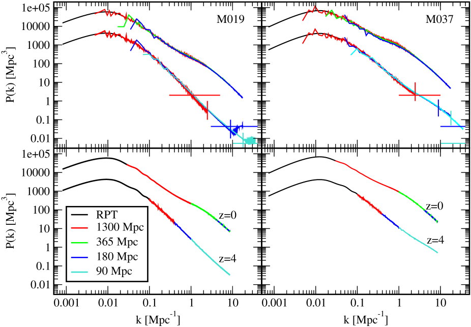
Figure 2 shows the matched power spectra for two example models, M019 and M037, representing the lowest and highest $\sigma_{8}$ in our model selection. The upper panels show the full power spectra from all boxes while the lower panels show the results with cut-offs applied at the appropriate $k$-values. The results in the lower panel demonstrate that the approach of using nested volumes is qualitatively satisfactory. In the next two sub-sections we discuss the main errors involved in the matching procedure, (i) finite mass resolution which leads us to push beyond $k_{\rm Ny}/2$ for the small boxes, and (ii) finite volume effects.

3.2 Finite mass resolution effects

In Heitmann et al. (2010) the effects of finite mass resolution on power spectrum estimation were discussed in some detail. Two effects investigated there act in opposite directions. The first is sampling noise, i.e., the effect on computing a power spectrum from a density field computed from a different number of particles. For this, a particle distribution at $z=0$ was down-sampled by factors of 8, 64, and 512 and the power spectra re-measured. The effect of the insufficient sampling of the density field led to an enhancement of the power spectrum larger than 1% beyond $k_{\rm Ny}/2$. The second is the effect of lower particle sampling in the initial conditions. This leads to a suppression of the power spectrum since the initial conditions now lack small-scale power. This effect decreases for simulations with larger Nyquist frequency since the number of modes in the box at small scales increases. In the test in Heitmann et al. (2010) it was shown that a simulation with $k_{\rm Ny}$=0.859 $h$Mpc^-1 has lost more than 10% of power at $k_{\rm Ny}/2$, while for $k_{\rm Ny}$=3.44 $h$Mpc^-1 it is well below 1% at $k_{\rm Ny}/2$.

In the current paper, we use the large volume simulations (1300 Mpc) only up to $k\leq 1~{}$Mpc^-1 at low redshift and $k\leq 0.4~{}$Mpc^-1 at high redshift, both values being well below $k_{\rm Ny}/2$. For the smallest volumes (90 Mpc) we also do not use any results beyond $k_{\rm Ny}/2$, simply because for the smallest boxes the Nyquist limit is much larger than $k\sim 10~{}$Mpc^-1. For the intermediate boxes (180 Mpc and 365 Mpc) we choose to be more aggressive. For the lowest redshifts we push the 365 Mpc limit to twice the Nyquist criterion and for intermediate redshifts we use the 180 Mpc box out to the Nyquist frequency. In principle, we could have avoided pushing the 365 Mpc box beyond the Nyquist limit by using the 180 Mpc box at large $k$ values instead. There are two reasons why we chose not to do this.

First, the comparison of inaccuracies due to finite box effects versus going beyond the Nyquist limit suggests that the finite box errors dominate. The quasi-linear regime in the small box simulations close to the final time step at which they are used is not accurate because of the missing large-scale power. In addition, the scatter in the overall amplitude is larger due to the small box size as discussed in the next sub-section. These two errors combine to outweigh the inaccuracy due to the Nyquist limit. This point is illustrated in Fig. 2. In the right upper panel (M037), at $z=0$, the green curve shows the result for the 365 Mpc box while the blue curve shows the result for the 180 Mpc box. It is apparent that the small box clearly does not capture the nonlinear turn-over behavior beyond $k\sim 0.1$ Mpc^-1 very well. On the other hand, both results are in close agreement at large $k$, so the accuracy of the 365 Mpc box results is still good at that point.

Second, the matching procedure described in Section 5 for melding the different power spectra pieces induces another small inaccuracy. This is again mainly due to finite box size effects, as the amplitude has to be adjusted to enable a matching of the boxes in the high $k$ region. It is therefore desirable to minimize the number of matching points, and hence to take the results from the 365 Mpc boxes out to higher $k$ values, rather than to introduce another matching point at intermediate scales. In order to verify that using the 365 Mpc box at higher $k$ does not introduce a major error, we also checked that the difference at high $k$ between the 365 Mpc box and the 180 Mpc box is small, as can be seen in Fig. 2. For M037 (high $\sigma_{8}$) we find differences of 2% and less beyond $k=6$ Mpc^-1 and for M019 (low $\sigma_{8}$) we find differences well below 1% in the high $k$ range.

To summarize this discussion, for the high redshift results, we do not use simulations beyond $k_{\rm Ny}/2$ (see Tables 5-5 for more details) and therefore estimate the error throughout the $k$ range as being well below 1%, based on the test results from Heitmann et al. (2010). For the low redshift cases, we use some results that go beyond the Nyquist limit. By comparing to the smaller boxes we estimate that the error does not exceed 2%.

3.3 Finite box size effects

Figure 3: Variations in power spectra due to different realizations from 127 simulations, each for a 325 Mpc box size. The upper panel shows the ratio of each of the 127 results at $z=0$ with respect to the average power spectrum. The lower panel shows an attempt to correct the results – here we adjust the amplitude of each power spectrum so that it matches the average power spectrum at the largest $k$-value. While at large $k$ this reduces the error somewhat, the procedure is not satisfactory overall and we do not use it in the final results. The scatter is roughly at the few percent level.

As outlined in the Introduction, ultimately one would want to carry out simulations in large box sizes, 1-2 Gpc, but this is currently impractical for a large suite of runs, each with sufficient mass resolution. Smaller simulation volumes have two drawbacks: (i) At redshifts close to $z=0$ the undersampling of large-scale power may be a problem (the precise extent depending on $\sigma_{8}$ and the box size). In smaller boxes, while the largest-scale modes might appear to be linear, their amplitude is actually suppressed by missing nonlinear power (in a large volume run, the same modes would have higher amplitudes). (ii) The realization scatter in small volumes is much larger due to the smaller number of large scale modes. The first of these points was considered in depth in Heitmann et al. (2010). There, we demonstrated the suppression of the power spectrum due to finite volume effects by comparing the average of 4 realizations in a 2000 $h^{-1}$Mpc box, 8 realizations in a 936 $h^{-1}$Mpc box, and 127 realizations in a a 234 $h^{-1}$Mpc box. Figure 6 in Heitmann et al. (2010) shows the suppression at mildly nonlinear scales. The realization scatter was not a significant issue in that paper since the final simulation volumes were large (1300 Mpc) and we averaged over 20 realizations.

Figure 4: Test of realization scatter on small scales. Shown are the results from six simulations that have the same realization on large scales but different realizations on small scales divided by the average of all six power spectra. The red line indicates the transition between the two regimes. Note that some of the realization noise from the small scales leaks back to larger scales.

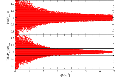
In the current paper, the realization scatter is of concern since we do resort to using small volumes. The mildly nonlinear regime is still very accurate since it is covered by large volume simulations, so the key question is to understand the high-$k$ behavior. In order to investigate this effect, we carry out two tests. First, we use the same 127 simulations used in Heitmann et al. (2010) to measure the overall dispersion in the power spectra between different realizations. These simulations were carried out in 325 Mpc volumes with a PM code almost matching the small simulation volumes used here. Since we are only interested in the relative effect, these lower resolution simulations are sufficient. The results are encapsulated in Fig. 3. The upper panel shows the ratio of the average of the 127 power spectra with respect to each individual spectrum; in the lower panel, we attempt to correct the run-to-run scatter by simply adjusting the amplitude of each power spectrum to the average value at the highest measured $k$ (which is well-sampled in each simulation). This procedure improves the scatter somewhat but is rather uncontrolled and we decided not to use it. Nevertheless, the result is somewhat interesting. Overall, the run-to-run scatter at small scales is up to about 5%, at the matching scale of $k\sim 1$ Mpc^-1, and up to 10% for the most extreme outliers. In order to reduce this problem, we carry out at least two realizations for each model, in some case up to four to obtain a realization in which the matching to the 1300 Mpc box is as close as possible. Since we match the even smaller volumes (180 Mpc and 90 Mpc) at larger $k$ values, the problem there is not quite as severe. Nevertheless, even in those cases we run up to four realizations per model to provide an accurate match to the larger boxes.

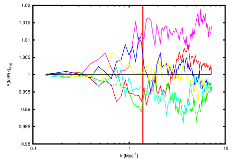
As a second check we carry out six simulations of the same cosmology each with box length $L=365~{}$Mpc and $N_{p}^{3}=512^{3}$ particles, which are chosen to exactly match the size and resolution of the smaller Coyote runs. The initial particle distribution is set with the same realization at $z=211$ on large scales for all six simulations, but on scales smaller than $k=1.39$ Mpc^-1, we allow the initial conditions to vary between runs by changing the random seed for each simulation. These are then evolved using Gadget-2 and we show the ratio of power spectra at $z=0$ with reference to a single simulation in the set in Fig. 4. The red line marks where the initial power spectrum differs between the realizations. Notice that the scatter in the power spectrum is less than $\sim 3\%$ and appears unbiased. This gives an estimate of the amount of mismatch between the 1300 Mpc and 365 Mpc Coyote simulations that we can expect after matching their power spectra. There is also a small amount of leakage of power from small to large scale modes, since the power spectra only match at $k\ll 1.39$ Mpc^-1, where they were seeded identically in the initial conditions.

In terms of the effects of the missing low-$k$ power, at z=0, for a $\sim 100$ Mpc box, the rms amplitude of the DC mode is at the level of $\sim 10$%, falling to a few percent at $\sim 300$ Mpc (see, e.g., Gnedin, Kravtsov, & Rudd 2011). These numbers are sufficiently small – given the level of accuracy we are aiming to attain here – that a more sophisticated correction procedure is not required. As previously mentioned, box sizes in the 1-2 Gpc range are sufficiently large to render these effects sub-dominant when targeting accuracy levels of $\sim 1$% Heitmann et al. (2010). As more computer power becomes available, construction of the next generation of emulators will profit from the increased volume and better mass resolution, both of which are essential to improve the accuracy at higher wavenumbers.

To summarize, finite box size effects are clearly an important issue. Some of the problems such as realization scatter can be overcome by generating a large number of realizations (though this is expensive) but some small inaccuracies in the power spectrum will be unavoidable until larger volume, high-particle loading simulations can be carried out.

4 Hubble Parameter Extension

In our original work, the value for the Hubble parameter was automatically determined from the other five cosmological parameters to be the best-fit CMB value. To allow for more flexibility, especially keeping in mind possible tensions in different observational values of $h$, we now aim to allow it to vary within the range that is covered by the original Coyote Universe runs, i.e., $0.55\leq h\leq 0.85$. This means that the sampled parameter space must be suitably extended.

A first idea might be to use the existing 37 models (all of which have different values of $h$) and rebuild the emulator keeping the Hubble parameter free. This naive approach is inadequate. Figure 6 in Heitmann et al. (2009) (seventh row) shows the distribution of $h$ values with respect to the other parameters. From that figure it is clear that the parameter space for $h$ is not well covered if we restrict ourselves to the 37 available models. The design has large holes, particularly for high values of $h$. Our tests confirmed that this sub-optimal design does not lead to an accurate emulator. We note that this result is in fact a successful demonstration of our overall approach, since it shows that the optimality of the sampling design is indeed a crucial factor.

Figure 5: Accuracy of the linear power spectrum emulator of the full six-dimensional parameter space. Shown is the ratio of the emulator to the linear power spectra for ten extra models not used for constructing the emulator itself. The error overall is within 1%. Note that we only included information on the Hubble parameter $h$ on large scales, with an upper cutoff at $k=0.03~{}$Mpc^-1.

The obvious alternate approach to include $h$ as a new parameter is to generate a new design over six parameters and increase the number of models to obtain sufficient accuracy. This is obviously undesirable for just one additional parameter since it would add a large computational cost and would not make use of the already available simulations. We therefore choose a quite different path.

The new idea implemented here is to exploit a certain flexibility in constructing emulators; this flexibility relates to the fact that emulators can be constructed by incorporating results from multiple models across different scales, i.e., where the result for each model does not necessarily have information available across the complete set of scales.

We proceed by generating 100 new predictions over a six-dimensional parameter space $\theta=\{\omega_{b},\omega_{m},n_{s},h,w,\sigma_{8}\}$ with RPT out to $k\leq 0.1~{}$Mpc^-1 for high redshift ($z\geq 2$) and out to $k\leq 0.03~{}$Mpc^-1 for low redshift ($z<2$). For larger $k$-values we use the results from the original 37 simulations for which we already have high-accuracy predictions in the nonlinear regime. The idea behind this approach is that a significant amount of information is readily available in the linear to mildly nonlinear regime covered by RPT. In addition, the very accurate predictions at low $k$, as provided by the 100 power spectra, helps to anchor the power spectra correctly on large scales. The information on small scales is then provided by the available 37 models that have been fully simulated.

Figure 6: Effects of the six different parameters within their respective prior ranges on the linear matter power spectrum. Shown is the ratio with respect to a model where each parameter is fixed at its median value: $\theta=\{0.0225,0.1375,0.95,0.7,-1.0,0.755\}$ and the sixth parameter (denoted at the top of each panel) is varied as a function of $k$ with $k_{0}$=1 Mpc^-1. Light blue colors show results for small values of the sixth parameter, while pink colors show results for large values. The change of the power spectrum when varying the Hubble parameter $h$ is independent of scale, the reason why in the case of the linear power spectrum the addition of $h$ as a free parameter works well, even when using information only on very large scales.

We modify the emulation procedure from Lawrence et al. (2010) to account for the inclusion of both ‘long’ power spectra over the entire $k$ range of interest and ‘short’ power spectra in the low $k$ range only. Recall that in Lawrence et al. (2010), the power spectra are modeled using a basis representation:

$$\mathcal{P}(k;z;\theta)=\sum_{i=1}^{n_{\mathcal{P}}}\phi_{i}(k;z)w_{i}(\theta),~{}~{}~{}\theta\in[0,1]^{n_{\mathcal{\theta}}},$$ (11)

where the $\phi_{i}(k;z)$ are the basis functions, the $w_{i}(\theta)$ are the corresponding weights, and the $\theta$ represent the cosmological parameters. The basis vectors are constructed from principal components and the weights are modeled as a Gaussian process. We again use Gaussian processes to model the weights, but construct the basis vectors slightly differently to better represent the variation in the long and short power spectra.

Two features inform our selection of basis vectors: the inclusion of RPT power spectra that cover only low $k$ and the combining of power spectra from $N$-body simulations that use different box sizes. First, we compute three principal component basis vectors using the 37 smoothed spectra resulting from combining $N$-body simulations of different sizes. Three basis vectors is sufficient to capture the systematic variation at high $k$ and the shorter RPT spectra yield well-behaved weights when projected on to these. Second, we remove the effects of the first three basis vectors and compute three additional PC basis vectors on the residuals of the 37 smoothed spectra, but only over the $k$ range of the original simulations. This improves the resulting prediction of spectra over this $k$ range, while avoiding extra variation at high $k$ resulting from the combination. Again, the residuals for the RPT power spectra project on these basis vectors in a well-behaved manner. Finally, we compute three additional basis vectors on the residuals from all 137 simulations over the $k$ range covered by the RPT power spectra. This further improves the modeling over this low $k$ region. For both sets of basis vectors that cover only part of the $k$ range, the basis vectors taper linearly to zero over their last 50 $k$ values to ensure continuity. This gives a total of nine basis vectors whose weights are modeled with a Gaussian process.

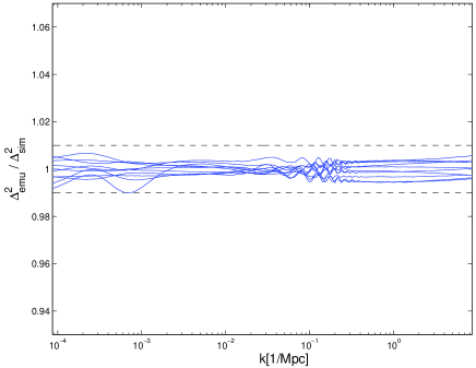
In order to test the build-strategy that allows us to combine a different number of simulations for small and large $k$, we carry out a test with the linear power spectrum. We generate 100 predictions for the linear power spectrum out to $k\leq 0.03~{}$Mpc^-1 and in addition 37 predictions following the original design over the full $k$ range out to $k\leq 10.0~{}$Mpc^-1. We then build an emulator over the full $k$ range allowing $h$ to vary. In order to test the accuracy of the new emulator, we generate a set of 10 additional power spectra over the full parameter range and compare the emulator prediction with those exact results. Figure 5 shows the ratio of the emulator prediction with the linear theory answer. Overall, the accuracy is around 1%, which is very satisfactory.

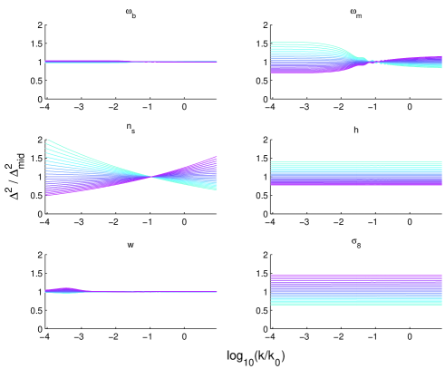
With the new emulator in hand, we briefly study the dependence of the power spectrum on the different cosmological parameters. For this we generate a set of sensitivity plots, shown in Fig. 6. The idea behind the sensitivity study is simple: we determine the power spectrum for a model in the center of the parameter hypercube and then vary one parameter at a time from its smallest to highest value. This illustrates concisely the effect of each parameter on the power spectrum on all scales studied. The Hubble parameter primarily shifts the amplitude of the power spectrum up and down (right panel, middle row), which explains why the simple addition scheme here works so well.

We also produce a second emulator that keeps $h$ fixed. This emulator does not use the additional RPT spectra, but does include the results from the smaller $N$-body simulations. This emulator was constructed in the usual manner, with $6$ PC basis functions computed from the 37 spectra over the whole $k$ range.

We will show in a future publication that the idea of combining different numbers of models at different length scales is also very useful in obtaining accurate predictions of the power spectrum on even smaller scales. As alluded to in the Introduction, computing power spectra on such scales is computationally very expensive. It is very helpful if the number of models needed for this can be kept to a minimum.

5 Smooth Power Spectrum Generation

The power spectra from the $N$-body simulations are smoothed with essentially the same process convolution model used in Lawrence et al. (2010), but with an important addition to account for vertical shifts where power spectra from different simulations are pasted together.

In Lawrence et al. (2010), the simulation of cosmology $c$, resolution $s$, and replicate $i$ produces a spectrum, $P^{c}_{s,i}$. We model this as a multivariate Gaussian variable with a known covariance $\Omega$, and a smooth mean described by a process convolution (Higdon, 2002). A process convolution is constructed by generating a latent stochastic process and smoothing it. In Lawrence et al. (2010), the spectra for each cosmology share a latent process, $u^{c}$, modeled as a Brownian motion observed on a sparse grid. These latent processes are smoothed by a common smoothing matrix, $K^{\sigma}$, made from Gaussian smoothing kernels whose kernel width varies across the domain in order to account for nonstationarity. The resulting model has a probability density function

$$f(P^{c}_{s,i}) \propto \left|A_{s}\Omega A_{s}^{\prime}\right|^{1/2}$$

$$\times \exp\left\{-\frac{1}{2}\left(P^{c}_{s,i}-A_{s}K^{\sigma}u^{c}\right)^{\prime}A_{s}\Omega A_{s}^{\prime}\left(P^{c}_{s,i}-A_{s}K^{\sigma}u^{c}\right),\right\},$$

where the matrix $A_{s}$ truncates the length of the spectrum depending on the resolution. The modeling details are given in Lawrence et al. (2010).

For the current work, we make a small addition to the mean function for the spectrum for each simulation. The spectra for the highest resolution simulations are augmented with spectra from the smaller boxes as described in the assembly tables. At each matching point, the spectra from each box may have a small vertical offset. However, we know that each simulation is approximating a smooth spectrum across the $k$ range. To account for this, we modify the mean structure for the simulation model. The mean structure is still built around a process convolution model, but includes additional terms that move each section of the simulated spectrum up or down.

Let $H^{c}$ be a matrix with a row for each $k$ value and three columns (one for each of the small boxes – no offset if estimated between the perturbation theory and the original set of simulations). Let the cosmology index $c$ also index redshift (although unstated, this is also true in Lawrence et al. 2010). This matrix describes the matching. At a particular $k$, if the simulated spectrum is represented by a result from perturbation theory or the original simulations, the matrix $H^{c}$ has a row of zeros. If the simulated spectrum uses the result from the 365 Mpc box, the row has a one in the first column. If the simulated spectrum uses a result from the 180 Mpc box or the 90 Mpc box, the row has a one in the second or third column respectively. Each can have at most a single non-zero entry. Let $b^{c}$ be a set of three coefficients that represent the offset of the simulated result from the unknown smooth mean. We add these terms to the model. Let $\mathcal{P}^{c}=K^{\sigma}u^{c}+H^{c}b^{c}$, which gives the density

$$f(P^{c}_{s,i}) \propto \left|A_{s}\Omega A_{s}^{\prime}\right|^{1/2}$$

$$\times \exp\left\{-\frac{1}{2}\left(P^{c}_{s,i}-A_{s}\mathcal{P}^{c}\right)^{\prime}A_{s}\Omega A_{s}^{\prime}\left(P^{c}_{s,i}-A_{s}\mathcal{P}^{c}\right)\right\}.$$

This model conveys the information that there is a smooth spectrum represented by $K^{\sigma}u^{c}$ and that we observe a noisy version of it that has vertical shifts over some ranges.

The offset parameters need a prior distribution to complete the specification. We give them a zero-mean Gaussian prior:

$$\pi(b)\propto\exp\left\{-\frac{\lambda_{b}}{2}b^{\prime}b\right\}.$$ (14)

The parameter $\lambda_{b}$ is a precision parameter that we set equal to the known precision of the simulated spectrum at the first matching point. Like the latent process $u^{c}$, the $b$ can be integrated out of the posterior and need not be drawn as part of the Markov chain Monte Carlo approach.

6 Emulator for the Matter Power Spectrum

Figure 7: Emulator predictions for the nonlinear power spectra for the best fit cosmologies for WMAP-7 and Planck (see text for details on the parameter choices) at $z=0$. Due to the higher values for $\omega_{m}$ and $\sigma_{8}$, the Planck results imply a noticeable change in the nonlinear regime.

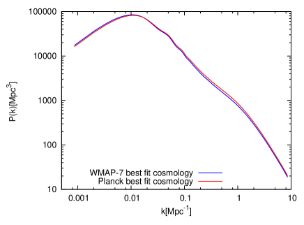
The construction of the new power spectrum emulator now follows the general methodology laid out in Heitmann et al. (2009) and Lawrence et al. (2010) with the small modifications discussed above to combine power spectra over different $k$ ranges. In this section we present some results from the emulator and tests of its accuracy. To start, we show the predictions of the emulator for the best-fit cosmology found by the WMAP-7 and Planck surveys in Fig. 7. Following the notation in Eq. (3) the parameters used are

$$\theta_{\rm\small WMAP-7} = \left\{0.0225,0.13328,0.97,0.7,-1.0,0.81\right\},$$ (15)

$$\theta_{\rm\small Planck} = \left\{0.02225,0.14026,0.968,0.6816,-1.0,0.8284\right\},$$

as obtained from CMB measurements alone. While the spectra are close, the Planck parameters lead to an enhancement of the power spectrum in the nonlinear regime.

Below we describe a number of tests of the emulator accuracy. We find that the emulator quality is better than 5% over a large $k$ and $z$ range, even when including the new free parameter, $h$. We also include a comparison against the latest improved version of Halofit as implemented in CAMB (see Takahashi et al. 2012 for details).

6.1 Power Spectrum Predictions

As explained in Section 2 the emulator is built using results from 37 cosmological models, specified in Table 1. In addition to these models, we have generated $P(k)$ results for a $\Lambda$CDM model (M000), which is close to the current best-fit measurements. Simulations for this model were carried out in exactly the same way as for the other models, using several realizations for each box size, and then matching them to produce a smoothed power spectrum. This reference $P(k)$ can be used as one test of the emulator’s accuracy.

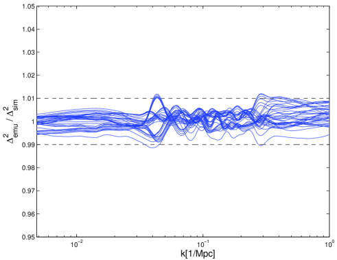
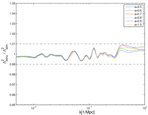
Figure 8 shows results for two emulator versions, one in which the value of $h$ is locked by the CMB distance to last scattering constraint for each model, as in the original emulator (Lawrence et al., 2010) (upper panel), and a second version where $h$ is allowed to be a free parameter following the approach presented in Section 4 (lower panel). Both panels show the ratio of the emulator to the simulation result as a function of $k$, the different solid curves correspond to eleven different redshifts between $z=4$ and $z=0$ used to build the emulator. In the $h$-fixed case, over a wide $k$ range, and for all redshifts, the emulator prediction is accurate at the 1% level, degrading slightly only at larger $k$ values, but still remaining better than 5%.

Figure 8: Accuracy of the emulator predictions for the reference $\Lambda$CDM model, M000, not used to construct the emulator. The ratio of the emulator prediction to the smoothed M000 simulation result is shown as a function of $k$. In the upper panel we show the predictions for the emulator with the Hubble parameter $h$ fixed to the best-fit CMB value for each model, in the lower panel, the results when $h$ is allowed to be an independent parameter. The different colors represent results at different redshifts: blue: $a=0.2$, green: $a=0.25$, red: $a=0.2857$, cyan: $a=0.3333$, purple: $a=0.4$, yellow: $a=0.5$, gray: $a=0.6$, blue: $a=0.7$, green: $a=0.8$, red: $a=0.9$, cyan: $a=1.0$. The sequence of $a$ values correspond to the redshifts, $z=4$, 3, 2.5, 2, 1.5, 1, 0.67, 0.43, 0.25, 0.11, 0.0. The dashed horizontal line indicates the $1\%$ accuracy limit. Allowing for $h$ to vary freely only mildly affects the emulator error behavior.

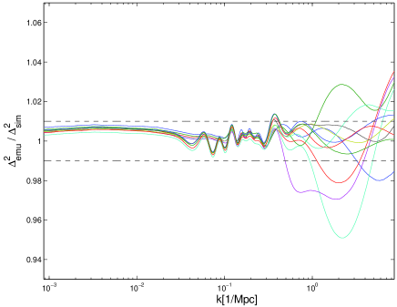
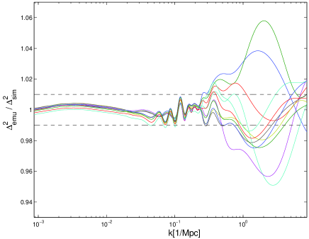
When $h$ is allowed to range freely (lower panel), then over the $k$ range where RPT is used (up to $k\sim 0.03~{}$Mpc^-1 for the low redshift results), the result is excellent, better than that in the top panel. This is not surprising since for this range we now have 100 models to predict the power spectrum. Beyond that matching point, the accuracy degrades slightly in the quasi-linear regime compared to the more restricted emulator, but is still around 1%. Finally, beyond $k\sim 1~{}$Mpc^-1, the predictions are less accurate, but the worst case error remains around 5%.

Figure 9: Holdout test for six models. For every test, the chosen model is excluded while building the emulator. The emulator prediction is then compared with that of the ‘held out’ model. The ratio of the emulator prediction to the smoothed simulation result for the six reference models is shown. As in Fig. 8, the top panel shows results with $h$-fixed emulators, while in the bottom panel, this constraint is relaxed. The different colors show results for different models (for each model we show results at all redshifts): blue: M004, green: M008, red: M013, cyan: M016, purple: M020, yellow: M026. The dashed horizontal line indicates the 1% accuracy limit, while the dashed vertical line shows $k=1$ Mpc^-1, the limit of our previous emulator (Lawrence et al., 2010).

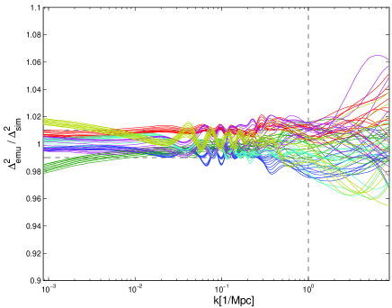
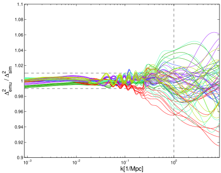
Next, we present results from a number of ‘holdout’ tests. In these tests, one model out of the 37 is excluded and an emulator is constructed based on the remaining 36 models. Then with this new emulator, a prediction for the excluded model is generated and the accuracy of the prediction determined. This test has an obvious caveat, particularly relevant in cases where not many models are available – degradation of the emulator quality because an important point in the parameter-space hypercube is omitted. This can be particularly serious if the excluded point is on the edge of the design, because now extrapolation to the edge of the hypercube is required, which has a much higher error. In order to avoid this additional complication, we restrict our holdout test to models that lie well within the hypercube. Nevertheless, it should be kept in mind that reported errors in the holdout tests can be larger than the actual values. The holdout test results, shown in Fig. 9 are similar to the ones found for M000, both in error amplitude and trends with increasing $k$. In the case where $h$ is allowed to be a free variable, the predictions are again less accurate, already in the quasi-linear regime, and degrade further beyond $k\sim 1~{}$Mpc^-1, to of order 5%. Note that the low-$k$ error band is consistent with that for the linear theory test case (Cf. Fig. 5).

To summarize, the accuracy of the new, extended, emulator is well-characterized at all redshifts. With $h$ fixed to the CMB constraint, the accuracy to $k\sim 1~{}$Mpc^-1 is at the $\sim 1\%$ level, degrading to $\sim 5\%$ for $k\sim 10~{}$Mpc^-1. When $h$ is allowed to be a free parameter, the degradation in accuracy is relatively modest.

In order to improve the accuracy of the emulator with $h$ included as a free parameter, a new design with more data points would have to be created. Based on the convergence tests in Habib et al. (2007), where the design space was varied between 32 and 128 models, a design with around 40 to 50 cosmological models should lead to percent level errors. We did not follow this strategy in the current paper because it would not allow us to use the simulation data already obtained in our previous work. Some of these questions (e.g., how to create nested designs that allow improvements of the emulator accuracy by adding more models in a systematic fashion) are currently under investigation, and will be addressed in future work.

6.2 Sensitivity Investigation

Figure 10: Same as in Fig. 6 but for the nonlinear power spectrum. The upper panel shows results at $z=4$ while the lower panel shows results at $z=0$.

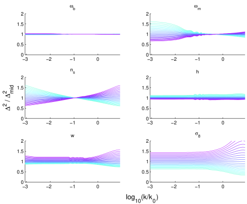
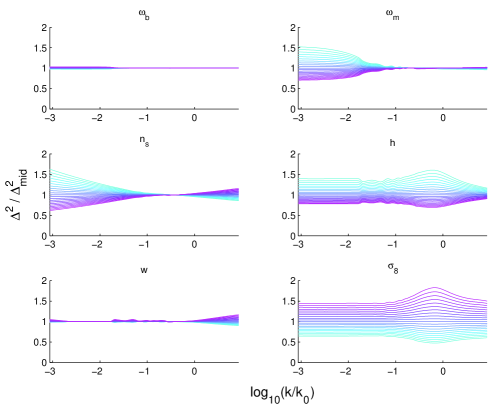
With the full emulator at hand we can now carry out a sensitivity analysis for the nonlinear power spectrum, along the same lines as conducted in Section 4 for the linear power spectrum. As before, we fix five of the six cosmological parameters at the midpoints of their range and then vary the sixth parameter between its minimum and maximum value. The results – for the lowest and highest redshift we consider – are shown in Fig. 10. The upper six panels show the results at $z=4$ and the lower six panels at $z=0$.

Some interesting features in the results can be noted. As to be expected, the baryon fraction $\omega_{b}$ does not affect the power spectrum significantly. The best constraints we have for $\omega_{b}$ come from CMB measurements; Planck determines this parameter to exquisite accuracy. The effect of the matter fraction $\omega_{m}$ dominates at large scales, here again, CMB results deliver very good estimates of this parameter. In general, it is important to allow for variations in $\omega_{m}$ due to degeneracy issues; $\omega_{m}$ influences the overall amplitude of the power spectrum as do $\sigma_{8}$ and $h$. The spectral index $n_{s}$, influencing the tilt of the power spectrum also mainly effects large scale behavior. The remaining three parameters, $h$, $w$, and in particular $\sigma_{8}$, alter the power spectrum on all scales and constraints on these parameters can therefore be improved by measurements of nonlinear scales.

In particular, the influence of $\sigma_{8}$ at the two redshifts shown in Fig. 10 on the power spectrum is noteworthy. At high redshift, nonlinearities for models with large $\sigma_{8}$ (pink) have already developed considerably, therefore the ratio with the midpoint power spectrum shows large values. The power spectra for small values of $\sigma_{8}$ (blue) show only mild nonlinear growth and therefore the ratio is still almost flat. Over time, the nonlinear turn-over moves in to smaller $k$ ranges (affecting larger and larger scales), causing the bump just before $k=1$ Mpc^-1 shown in the panel for $z=0$. At this epoch the overall difference between the models has decreased, since at this point all models have reached the nonlinear regime. A similar observation can be made for $w$ – at early times the differences between the models are more pronounced than at later times. It is easy to imagine using the new emulator as a convenient tool to investigate the effects of varying cosmological parameters and redshift on $P(k)$ in the nonlinear regime.

6.3 Comparison with Halofit

Figure 11: Performance of the emulator in comparison with Halofit from Takahashi et al. (2012) for M000 at $z=0$. Shown are the ratios of the emulator with fixed Hubble parameter and the smoothed simulation (blue), with the free Hubble parameter emulator (red), and with Halofit (black). (The emulator results are shown also in Fig. 8 in cyan and are here repeated for easy comparison with Halofit). The $h$-fixed emulator is accurate at the percent level out to $k\sim 1~{}$Mpc^-1 and at the 2% level at higher $k$, the $h$-free emulator is accurate at the 2% level throughout. Halofit on the other hand shows deviations at the 3% level at $k\sim 0.1~{}$Mpc^-1 and up to 6% in the higher $k$ regime.

Figure 12: Performance of the emulator in comparison with linear theory (dotted) supplied by CAMB and Halofit from Takahashi et al. (2012) (solid). Unless otherwise stated in the legend, the cosmological parameters are: $\omega_{m}=0.1296,\omega_{b}=0.0224,n_{s}=0.97,\sigma_{8}=0.8,w=-1,h=0.72$. The parameters for WMAP-7 and Planck are given in Eq. (15). See text for discussion.

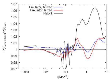
We now perform a comparison between the emulator and Halofit, a popular fitting formula for the matter power spectrum motivated by the halo model. We use the updated version with 35 fitting parameters provided by Takahashi et al. (2012), which is calibrated to larger volume and higher resolution N-body simulations than the original Smith et al. (2003) formula. It is based on simulations run on six WMAP cosmologies (years 1, 3, 5, 7, and two WMAP7 models, but with $w=-0.8$ and $w=-1.2$, instead of $w=-1$). The obtained fitting formula was checked against simulations run using the first 10 of the 37 Coyote models. This improved version of Halofit is stated to be accurate to $\sim 5\%$ in the range $0<k<1$ $h$Mpc^-1 and $\sim 10\%$ at $1<k<10$ $h$Mpc^-1, for $0<z<3$.

One important feature of the emulator-based approach is that, close to the parameter values of the underlying simulations, the emulator error is small, if not essentially the simulation error. However, this is not the case with a fitting formula. For instance, even though the N-body simulations that underlie the new Halofit formula agree with the original Coyote emulator at the $\sim 1-2\%$ level over its range of validity for the 10 Coyote models used as a reference in Takahashi et al. (2012) (se Fig. 2 of the cited reference), this good level of agreement drops to 8-13% (as a function of the $k$ range) when the fitting formula is used in the comparison. Depending on what one may be trying to achieve, this loss of accuracy in Halofit is significant.

We first compare the predictions of the emulator (both versions, $h$ free and $h$ fixed) at $z=0$ for M000 against the smooth simulations (in the same way as shown in Fig. 8) and the prediction of Halofit for the same model. Since the emulator was built without including this simulation, this is a good test of both prediction schemes, emulator and Halofit. The results are shown in Fig. 11. The emulator predictions for the $h$-fixed version are accurate at 1% out to $k\sim 1~{}$Mpc^-1 and then degrade very slightly to 2%. The $h$-free version of the emulator is accurate at the 1-2% level throughout. Halofit shows 3% deviations compared to the simulation in the mildly nonlinear regime ($k\sim 0.1~{}$Mpc^-1) and more than 6% in the nonlinear regime.

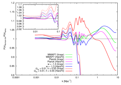
Next we show a comparison of the emulator ($h$-free version only) directly with Halofit for a variety of cosmologies at $z=0$. Figure 12 displays the ratio of the emulator with respect to linear theory power spectra from CAMB and Halofit as modified by Takahashi et al. (2012). We choose to test a WMAP7 (Komatsu et al., 2011) and a Planck (Ade et al., 2013) cosmology and two other cosmologies on the limits of the design of our emulator. The red and blue curves in particular are on the edge of the new design with $h$ as a free parameter. The cosmological parameters for these two model are the same as model M000: $\omega_{m}=0.1296,\omega_{b}=0.0224,n_{s}=0.97,\sigma_{8}=0.8,w=-1,h=0.72$ and in our comparison we vary one to two parameters at a time as noted on the legend.

At large scales, $k<0.01$ $h$Mpc^-1, all power spectra are consistent at the percent level; this is less trivial than it seems since Halofit and linear theory start diverging at $k\sim 0.003$ $h$Mpc^-1 and we use the full version of the emulator with extreme values of $h$ located at the edge of the design. On quasi-linear scales, there is $\sim 5$% deviation with some oscillatory structure from the BAO feature. On smaller scales, the accuracy is consistent with what is stated in Takahashi et al. (2012), apart from the matter dominated case with $\Omega_{m}$ = 0.51, in which the Halofit power spectrum is suppressed by more than 20%. The relatively uniform error behavior of an emulator – a result of the sampling theory and the Gaussian process based-regression methodology – is hard to reproduce in a fitting formula; the last result of the comparison provides an example of this.

7 Conclusion and Outlook

High accuracy predictions for cosmological observables in the nonlinear regime will be crucial in the future to exploit the power of ongoing and upcoming cosmological surveys. These predictions have to at least match, better yet, exceed the accuracy of the measurements themselves. Achieving this goal with first principles predictions or perturbation theory is impossible because of the highly nonlinear and dynamical nature of the problem. High-accuracy predictions must therefore be obtained from state of the art simulations.

In a series of recent papers (the Coyote Universe papers) we have shown how to build a prediction tool from a relatively small set of simulations (37 cosmological models) to generate the matter power spectrum out to $k\sim 1$ Mpc^-1 at the 1% accuracy out to $z=1$. In the current paper, using what we consider the ‘minimal’ amount of work, we have extended the emulator to significantly higher values of redshift and wavenumber. In addition, we have added one new free parameter, $h$.

With current computational resources, it is impossible to obtain high emulation accuracy out to large $k$ with a collection of single-box simulations, because the dynamic range requirements impose a very high computational cost. The use of nested boxes avoids the computational cost, at the expense of reduced accuracy, resulting from increased sampling variance as well as reduced accuracy in the region of the nonlinear turnover. Nevertheless, with this approach we have improved on the accuracy attained by any other existing prediction tool. Overall, our predictions for the power spectrum are accurate to better than 5%, and over smaller $k$ ranges around 1%, for $0<z<4$. In the high-$k$ regime, baryonic effects will have to be included in any case, so any future strategy should include methods for improving the accuracy of the gravity-only simulation results, as well as ways to model the baryonic contributions.

In a companion paper we will present a method for extrapolating the results beyond $k\sim 10$ Mpc^-1 (including estimates of the associated errors) and an emulator for the shear power spectrum and other weak lensing observables. More detailed work relevant for surveys (DES, LSST) is also underway.

For future surveys, the cosmological parameter space will have to be enlarged beyond what was considered here. In the case of DES, for example, predictions for dynamical dark energy models are needed. Increasing the sample space will further increase the associated computational costs. On the positive side, results from surveys such as Planck help to narrow down the parameter ranges substantially, which in turn will help to reduce the number of models we have to investigate. Multi-level sampling schemes can be devised to deal with these situations, one of our directions for future work.

Appendix A Appendix A: Test of the New Emulator Against Large High-resolution HACC Simulation

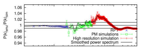
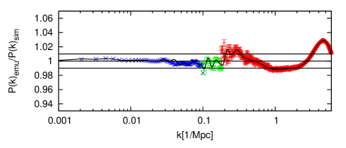
In this Appendix we present an additional test of our new $h$-free emulator set-up by using a simulation that covers a large range of the $k$ values of interest and uses a different N-body code, namely HACC (Hardware/Hybrid Accelerated Cosmology Code) (Habib et al., 2012). The cosmology for this test is the best-fit WMAP-7 cosmology ($\omega_{m}=0.1335,~{}\omega_{b}=0.02258,~{}n_{s}=0.963~{},w=-1.0,~{}\sigma_{8}=0.8~{},h=0.71$). With this final test we demonstrate that (i) the matching strategy described in Section 3.1 works well at the accuracy reported in the paper, (ii) the smoothing procedure described in Section 5 does not introduce any biases, and that (iii) the power spectrum calculation is robust under different N-body implementations. The last point had already been made in the Coyote-I paper (Heitmann et al. 2010) by comparing Gadget-2 results with the ART code (see Fig. 4 in Heitmann et al. 2010), and is here again confirmed with a third code out to higher $k$ values.

We show results for three redshifts, $z=0,1,2$ – at higher redshifts the large simulation volume leads to excess particle shot noise in the higher $k$ regime which is of most interest for this test. We cover a $k$ range between 0.001 to 6 Mpc^-1 via (i) renormalized perturbation theory out to $k\sim 0.04$ Mpc^-1 for $z=0,~{}1$ and $k\sim 0.14$ Mpc^-1 for $z=2$ as in the main paper; (ii) 16 realizations of PM simulations with 512³ particles on a 1024³ grid in a (1300 Mpc)³ volume out to $k\sim 0.25$ Mpc^-1 also as in the main paper; (iii) a (2100Mpc)³ volume, high-resolution simulation with 3200³ particles and 6.5 kpc force resolution to cover the remaining $k$-range. The difference with the main paper arises in the intermediate regime, where we drop the second set of PM simulations since the high-resolution simulation covers a significantly larger volume than the Gadget-2 runs. The realization scatter for the smaller $k$ values is reduced to a low-enough level that the single simulation spans the quasi-linear regime. Figure 13 shows the comparison of the emulator with the unsmoothed and smoothed simulations. This figure should be compared to Fig. 8, lower panel, where we show a similar cosmology (M000) but using the matching strategy of different size simulations that has been employed throughout the paper. The error level is very similar in both cases, demonstrating very good performance of the matching and smoothing strategy, as well as excellent agreement between HACC and Gadget-2.

Figure 13: Comparison of the $h$-free emulator with raw simulations, i.e., with no smoothing applied at three redshifts (upper panel: $z=0$, middle panel: $z=1$, lower panel: $z=2$). We show the results from resummed perturbation theory in blue, the average of 16 PM runs in green, and the result from one high resolution simulation in red. The black lines show the result from matching and smoothing all three pieces following the procedure described in detail in Section 5. Error bars describe the error in the simulations due to the finite number of modes, or cosmic variance. The predictions are well within the expected accuracy of the emulator.

Appendix B Appendix B: Improvement of Original Emulator

In the course of the work presented in this paper, some changes were made to previous versions of the CosmicEmu from Lawrence et al. (2010).

First, Taruya et al. (2012) present work on perturbation theory and compare their results to the CosmicEmu for the cosmologies that were simulated to build the CosmicEmu. Overall, they note a close match, but for M015, they find a notable difference. In the course of investigating this issue, we discovered a typographical error in the input files that were used to build the CosmicEmu. The file containing the input parameters differed from the input parameters used to run the actual simulations for three cosmologies: M015, M017, and M019. The effects of this error were quite local to the neighborhood of these three cosmologies.

Second, we experimented with the prior parameters for the Gaussian process emulation procedure. In order to explain this more fully, we must describe one more subtle detail in Gaussian process fitting. Appendix B in Heitmann et al. (2009) describes the statistical model for the Gaussian process emulation. Equation B1 in Heitmann et al. (2009) gives the Gaussian process distribution for the principal component weights with covariance matrix $\Sigma=\lambda_{w_{i}}^{-1}R(\theta,\theta^{\prime};\rho_{w_{i}})$. The function $R(\cdot)$, given in Equation B2, results in a response that interpolates and is extremely smooth. As a result, the model can be susceptible to estimation problems and overfitting. Thus, in practice, we include an additional term in the covariance specification to relax the interpolation requirement slightly. The actual covariance is given by $\Sigma=\lambda_{w_{i}}^{-1}R(\theta,\theta^{\prime};\rho_{w_{i}})+\lambda_{nug}^{-1}I$, where $I$ is the identity matrix. The new parameter $\lambda_{nug}$ is an additional precision term (the ‘nugget’) that governs how well the estimated response function interpolates the data. When this parameter is large, the response surface interpolates better. We estimate this parameter along with all of the others, so the data can inform about the smoothness of the model. Like the other precision parameters described in Heitmann et al. (2009), it has a Gamma prior distribution (see Equation B5 for an example). Unfortunately, the default prior parameters in the estimation software can prevent these precisions from being as large as the data would allow and prevent the response surface from capturing all of the behavior of the simulations. We now set these parameters at $a_{nug,i}=1$ and $b_{nug,i}=0$ where $i$ indexes the principal components. This prior gives the data much more control over the parameter estimate. The new estimates for $\lambda_{nug}$ are significantly larger than the previous estimates. The resulting response surface for each principal component basis is more accurate and more principal component basis functions can be used (seven instead of five).

Figure 14 shows the results of these two improvements on the holdout predictions and the prediction for the best fit cosmology M000. The fits, while good before, are now further improved.

Figure 14: Holdout (top) and M000 (bottom) results for the improved fit to the original CosmicEmu described in Lawrence et al. (2010). Compare to Figures 9 and 10 in that paper.

References

- Abell et al. (2009) Abell, P.A. et al. [LSST Science Collaborations and LSST Project Collaboration], arXiv:0912.0201 [astro-ph.IM]
- Ade et al. (2013) Ade, P.A.R. et al. [ Planck Collaboration], arXiv:1303.5076 [astro-ph.CO]
- Agarwal et al. (2012) Agarwal, S., Abdalla, F., Feldman, H., Lahav, O., & Thomas, S.A. 2012, MNRAS, 424, 1409
- Baugh, Gaztanaga, & Efstathiou (1995) Baugh, C.M., Gaztanaga, E., & Efstathiou, G. 1995, MNRAS, 274, 1049
- Bhattacharya et al. (2011) Bhattacharya, S., Heitmann, K., White, M., Lukić, Z., Wagner, C., & Habib, S. 2011, ApJ, 732, 211
- Bird, Viel, & Haehnelt (2012) Bird, S., Viel, M., & Haehnelt, M.G. 2012, MNRAS, 420, 2551
- Carlson, White, & Padmanabhan (2009) Carlson, J., White, M., & Padmanabhan, N. 2009, Phys. Rev. D80, 043531
- Cunha & Evrard (2010) Cunha, C.E. & Evrard, A.E. 2010, Phys. Rev. D., 81, 083509
- Crocce & Scoccimarro (2006) Crocce, M. & Scoccimarro, R. 2006, Phys. Rev. D73, 063519
- Crocce & Scoccimarro (2008) Crocce, M. & Scoccimarro, R. 2008, Phys. Rev. D77, 023533
- Das et al. (2012) Das, S. et al. 2011, Phys. Rev. Lett., 107, 021301
- de Jong et al. (2013) de Jong, J.T.A, et al. 2013, Experimental Astronomy, 35, 25
- Drinkwater et al. (2010) Drinkwater, M.J. et al. 2010, MNRAS, 401, 1429
- Gnedin, Kravtsov, & Rudd (2011) Gnedin, N.Y., Kravtzov, A.V., & Rudd, D.H. 2011, ApJS, 194, 46
- Eifler (2011) Eifler, T. 2011, MNRAS, 418, 536
- Habib et al. (2007) Habib, S., Heitmann, K., Higdon, D., Nakhleh, C., & Williams, B. 2007, Phys. Rev. D, 76, 083503
- Habib et al. (2012) Habib, S., Morozov, V., Finkel, H., Pope, A., Heitmann, K., Kumaran, K., Peterka, T., Insley, J., Daniel, D., Fasel, P., Frontiere, N., & Lukić, Z. 2012, Proc. SC12, arXiv:1211.4864
- Hearin & Zentner (2011) Hearin, A., Zentner, A.R., & Ma, Z. 2012, JCAP, 1204, 034
- Heitmann et al. (2006) Heitmann, K., Higdon, D., Nakhleh, C., & Habib, S. 2006, ApJ, 646, L1
- Heitmann et al. (2009) Heitmann K., Higdon D., White M., Habib S., Williams, B.J., & Wagner, C. 2009, ApJ, 705, 156
- Heitmann et al. (2010) Heitmann K., White M., Wagner C., Habib S., & Higdon D. 2010, ApJ, 715, 104
- Higdon (2002) Higdon, D. 2002, in Quantitative Methods for Current Environmental Issues, Space and Space-Time Modeling using Process Convolutions, ed. C. Anderson, V. Barnet, R.C. Chatwin, & A.H. El-Shaarawi (Berlin: Springer), 37
- Huff et al. (2011) Huff, E.M., Eifler, T., Hirata, M., Mandelbaum, R., Schlegel, D., & Seljak, U. 2011, arXiv:1112.3143 [astro-ph.CO]
- Huterer & Takada (2005) Huterer, D. & Takada, M. 2005, Astropart. Phys. 23, 369
- Jee et al. (2013) Jee, M. J., Tyson, J. A., Schneider, M.D., Wittman, D., Schmidt, S., & Hilbert, S. 2013, ApJ, 765, 26
- Jenkins et al. (2001) Jenkins, A. et al. 2001, MNRAS 321, 372
- Jing et al. (2006) Jing, Y.P., Zhang, P., Lin W.P., Gao L., & Springel V. 2006, ApJ, 640, L119
- Kilbinger et al. (2012) Kilbinger, M. et al. 2012, arXiv:1212.3338 [astro-ph.CO]
- Komatsu et al. (2011) Komatsu, E. et al. 2011, ApJS, 192, 18
- Kwan et al. (2013) Kwan, J., Bhattacharya, S., Heitmann, K., & Habib, S. 2013, ApJ, 768, 123
- Lawrence et al. (2010) Lawrence, E., Heitmann, K., White M., Higdon D., Wagner C., Habib S., & Williams, B. 2010, ApJ, 713, 1322
- Li & Ye (2000) Li, W. & Ye, K.Q. 2000, Journal of Statistical Planning and Inference, 90, 145
- Lin et al. (2011) Lin, H.; Dodelson, S., Seo, H.-J., Soares-Santos, M., Annis, J., Hao, J., Johnston, D., Kubo, J.M., Reis, R.R.R., & Simet, M. 2012, ApJ, 761, 15
- Merloni et al. (2012) Merloni, A. et al. 2012, arXiv:1209.3114 [astro-ph.CO]
- Peacock & Dodds (1996) Peacock, J.A. & Dodds, S.J. 1996, MNRAS, 280, L19
- Perlmutter et al. (1999) Perlmutter, S. et al. 1999, ApJ, 517, 565
- Refregier et al. (2010) Refregier, A., Amara, A., Kitching, T.D., Rassat, A., Scaramella, R., Weller, J. for the Euclid Imaging Consortium, 2010, arXiv:1001.0061 [astro-ph.IM]
- Riess et al. (1998) Riess, A.G. et al. 1998, AJ, 116, 1009
- Riess et al. (2011) Riess, A.G. et al. 2011, ApJ, 730, 119
- Rudd et al. (2008) Rudd, D., Zentner, A., & Kravtsov, A. 2008, ApJ, 672, 19
- Santner et al. (2003) Santner, T.J., Williams, B.J., & Notz, W.I. 2003, The Design and Analysis of Computer Experiments, Springer, New York
- Schlegel, White, & Eisenstein (2009) Schlegel, D., White, M. & Eisenstein, D. arXiv:0902.4680 [astro-ph.CO]
- Schneider et al. (2008) Schneider, M., Knox, L., Habib, S., Heitmann, K., Higdon, D., & Nakhleh, C. 2008, Phys. Rev. D, 78, 063529
- Schneider, Holm, & Knox (2011) Schneider, M., Holm, O., & Knox, L., 2011, ApJ, 728, 137
- Semboloni et al. (2006) Semboloni, E., Mellier, Y., van Waerbeke, L., Hoekstra, H., Tereno, I., Benabed, K., Gwyn, S.D.J., Fu, L., Hudson, M.J.; Maoli, R., & Parker, L.C. 2006, A&A, 452, 51
- Semboloni et al. (2011) Semboloni, E., Hoekstra, H., Schaye, J., van Daalen, M.P., & McCarthy, I.G. 2011, MNRAS 417, 2020
- Smith et al. (2003) Smith, R.E. et al. [The Virgo Consortium Collaboration], 2003, MNRAS 341, 1311
- Springel (2005) Springel, V. 2005, MNRAS, 364, 1105
- Sugai (2012) Sugai, H. et al. arXiv:1210.2719 [astro-ph.IM]
- Takahashi et al. (2012) Takahashi, R., Sato, M., Nishimichi, T., Taruya, A., & Oguri, M. 2012, ApJ, 761, 152
- Taruya et al. (2012) Taruya, A., Bernardeau, F., Nishimichi, T., & Codis S. 2012, Phys. Rev. D 86, 103528
- van Daalen et al. (2011) van Daalen, M.P., Schaye, J., Booth C.M., & Vecchia C.D. 2011, MNRAS, 415, 3649
- van Engelen et al. (2012) van Engelen, A. et al. 2012, ApJ, 756, 142
- Vikhlinin et al. (2009) Vikhlinin, A., Kravtsov, A.V., Burenin, R.A., Ebeling, H., Forman, W.R., Hornstrup, A., Jones, C., Murray, S.S., Nagai, D., Quintana, H., & Voevodkin, A. 2009, ApJ, 692, 1060
- Weinberg et al. (2012) Weinberg, D.H., Mortonson, M.J., Eisenstein, D.J., Hirata, C., Riess, A.G., & Rozo, E. 2012, arXiv:1201.2434 [astro-ph.CO]
- White (2004) White, M. 2004, Astropart. Phys., 22, 211
- Wu, Zentner, & Wechsler (2010) Wu, H.-Y., Zenter, A.R., & Wechsler, R. 2010, ApJ, 713, 856
- Zehavi et al. (2011) Zehavi, I. et al. 2011, ApJ, 726, 13
- Zentner et al. (2012) Zentner, A.R., Semboloni, E., Dodelson, S., Eifler, T., Krause, E., & Hearin, A.P. 2012, arXiv:1212.1177 [astro-ph.CO]
- Zhan & Knox (2004) Zhan, H. & Knox, L. 2004, ApJ, 616, L75