Information-theoretic tools for parametrized coarse-graining of non-equilibrium extended systems

Abstract

In this paper we focus on the development of new methods suitable for efficient and reliable coarse-graining of non-equilibrium molecular systems. In this context, we propose error estimation and controlled-fidelity model reduction methods based on Path-Space Information Theory, combined with statistical parametric estimation of rates for non-equilibrium stationary processes. The approach we propose extends the applicability of existing information-based methods for deriving parametrized coarse-grained models to Non-Equilibrium systems with Stationary States (NESS). In the context of coarse-graining it allows for constructing optimal parametrized Markovian coarse-grained dynamics within a parametric family, by minimizing information loss (due to coarse-graining) on the path space. Furthermore, we propose an asymptotically equivalent method–related to maximum likelihood estimators for stochastic processes–where the coarse-graining is obtained by optimizing the information content in path space of the coarse variables, with respect to the projected computational data from a fine-scale simulation. Finally, the associated path-space Fisher Information Matrix can provide confidence intervals for the corresponding parameter estimators. We demonstrate the proposed coarse-graining method in (a) non-equilibrium systems with diffusing interacting particles, driven by out-of-equilibrium boundary conditions, as well as (b) multi-scale diffusions and their well-studied corresponding stochastic averaging limits, comparing them to our proposed methodologies.

I Introduction

Non-equilibrium systems at transient or steady state regimes are typical in applied science and engineering, and are the result of coupling between different physicochemical mechanisms, driven by external couplings or boundary conditions. Typical examples include reaction-diffusion systems in heteroepitaxial catalytic materials, polymeric flows and separation processes in microporous materials, Stamatakis and Vlachos (2012); Padding and Briels (2011); Smit and Maesen (2008). In this paper we develop reliable model-reduction methods, i.e., having controlled fidelity of approximation, and capable to handle extended, non-equilibrium statistical mechanics models. These coarse-graining methods allow for constructing optimal parametrized Markovian coarse-grained dynamics within a parametric family, by minimizing information loss (due to coarse-graining) on the path space. Model-reduction (or coarse-graining) approaches can be often described in the context of parameter estimation in parametrized statistical models. However, atomistic models of materials lead to high-dimensional probability distributions and/or stochastic processes to which the standard methods of statistical inference and model discrimination are not directly applicable. The emphasis on information theory tools is also partly justified since often we are interested in probability density functions (PDF), typically non-Gaussian, due to the significance of tail events in complex systems. A primary focus of this paper is on systems with Non-Equilibrium Steady States (NESS), i.e., systems in which a steady state is reached but the detailed balance condition is violated and explicit formulas for the stationary distribution, e.g., in the form of a Gibbs distribution, are not available.

Information-theoretic methods for the analysis of stochastic models typically employ entropy-based tools for analyzing and estimating a distance between (probability) measures. In particular, the relative entropy (Kullback-Leibler divergence) of two probability measures $\mu(dx)=\mu(x)\,dx$ and $\nu(dx)=\nu(x)\,dx$

$$\mathcal{R}\left({\mu}{\,|\,}{\nu}\right)=\int\mu(x)\log\frac{\mu(x)}{\nu(x)}\,dx$$

allows us to define a pseudo-distance between two measures. A key property of the relative entropy $\mathcal{R}\left({P}{\,|\,}{Q}\right)$ is that $\mathcal{R}\left({P}{\,|\,}{Q}\right)\geq 0$ with equality if and only if $P=Q$, which allows us to view relative entropy as a “distance” (more precisely a semi-metric) between two probability measures $P$ and $Q$. Moreover, from an information theory perspective Cover and Thomas (1991), the relative entropy measures loss/change of information. Relative entropy for high-dimensional systems was used as measure of loss of information in coarse-graining Katsoulakis and Trashorras (2006); Katsoulakis et al. (2007); Arnst and Ghanem (2008), and sensitivity analysis for climate modeling problems Majda and Gershgorin (2010).

Using entropy-based analytical tools has proved essential for deriving rigorous results for passage from interacting particle models to mean-field descriptions, Kipnis and Landim (1999). The application of relative entropy methods to the error analysis of coarse-graining of stochastic particle systems have been introduced and studied in Katsoulakis et al. (2007, 2008, 2013); Katsoulakis, Majda, and Vlachos (2003); Katsoulakis and Vlachos (2003). Aside of this rigorous numerical analysis direction, entropy-based computational techniques were also developed and used for constructing approximations of coarse-grained (effective) potentials for models of large biomolecules and polymeric systems (fluids, melts). Optimal parametrization of effective potentials based on minimizing the relative entropy between equilibrium Gibbs states, e.g.,Chaimovich and Shell (2011); Carmichael and Shell (2012); Bilionis and Zabaras (2012), extended previously developed inverse Monte Carlo methods, primarily based on force matching approaches, used in coarse-graining of macromolecules (see, e.g., Tschöp et al. (1998); Müller-Plathe (2002)). In Espanol and Zuniga (2011) an extension to dynamics is proposed in the context of Fokker-Planck equations, by considering the corresponding relative entropy for discrete-time approximations of the transition probabilities. Furthermore, relative entropy was used as means to improve model fidelity in a parametric, multi-model approximation framework of complex dynamical systems, at least when the model’s steady-state distributions are explicitly known, Majda and Gershgorin (2011). Overall, such parametrization techniques are focusing on systems with a known steady state, such as a Gibbs equilibrium distribution. More specifically, computational implementations of optimal parametrization in the inverse Monte Carlo methods is relatively straightforward for equilibrium systems in which the best-fit procedure is applied to an explicitly known equilibrium distribution and where relative entropy is explicitly computable.

On the other hand, this is not the case in non-equilibrium systems, even at a steady state where typically we do not have a Gibbs structure and the steady-state distribution is unknown altogether, setting up one of the primary challenges for this paper. Indeed, here we show that, in non-equilibrium systems the general information theory ideas based on Kullback-Leibler divergence are still applicable but they have to be properly formulated in the context of Non-equilibrium Statistical Mechanics by focusing on the probability distribution of the entire time series, i.e., on the path space of the underlying stochastic processes. We show that, surprisingly, such a path-space relative entropy formulation is: (a) general in the sense that it applies to any Markovian models (e.g. Langevin dynamics, Kinetic Monte Carlo, etc), and (b) is easily computable as an ergodic average in terms of the Relative Entropy Rate  (RER), therefore allowing us to construct optimal parametrized Markovian coarse-grained dynamics for large classes of models. This procedure involves the minimization of information loss in path space, where information is inadvertently lost due to coarse-graining procedure. In fact, the proposed parametrization scheme in Espanol and Zuniga (2011) is mathematically justified by reformulating it on the path space using the Relative Entropy Rate and it is a specific, but reversible (i.e., it has a Gibbs steady state) example of our methodology. Furthermore, we propose an asymptotically equivalent method to RER minimization, which is related to to maximum likelihood estimators for stochastic processes, and where the optimal coarse-graining is obtained by optimizing the information content in path space of the coarse variables, with respect to the projected computational data from a fine-scale simulation. Finally, the path-space Fisher Information Matrix (FIM) derived from Relative Entropy Rate (RER) can provide confidence intervals for the corresponding statistical estimators of the optimal parameter obtained through the minimization problem.

The Relative Entropy Rate (RER) was earlier proposed as a (pseudo) metric in order to evaluate the convergence of adaptive sampling schemes for Markov State Models (MSM)Bowman, Ensign, and Pande (2010); the proposed coarse-graining perspective, which is related to Maximum Likelihood Estimators (MLE), e.g., (31), could provide new insights in comparing MSMs since it only requires fine-scale data–and not explicitly a fine-scale MSM for estimating the RER. Furthermore, RER and in particular the path-space FIM where introduced recently as gradient-free sensitivity analysis tools for complex, non-equilibrium stochastic systems with a wide range of applicability to reaction networks, lattice Kinetic Monte Carlo and Langevin dynamics Pantazis and Katsoulakis (2013). Unlike the coarse-graining setting we propose here and where models are set in different state spaces depending on their granularity, in the latter work the same state space is assumed between compared models.

The paper is structured as follows. In Section II we formulate the path-space information theory tools used in the paper, including the key concept of Relative Entropy Rate. In Section III we present the parameterization method of coarse-grained dynamics and the connections with maximum likelihood estimators and the Fisher Information Matrix. In Section IV we briefly discuss statistical estimators for RER and FIM. Finally, in Section V we demonstrate the proposed coarse-graining method in (a) non-equilibrium systems with diffusing interacting particles, driven by out-of-equilibrium boundary conditions, as well as (b) multi-scale diffusions and their well-studied corresponding stochastic averaging limits, comparing them to our proposed methodologies.

II Relative Entropy Rate, path space information theory and error quantification for non-equilibrium systems

First, we formulate a general entropy-based error analysis for coarse-graining, dimensional reduction and parametrization of high-dimensional Markov processes, simulated by Kinetic Monte Carlo (KMC) and Langevin Dynamics. Typically such systems have Non-Equilibrium Steady States (NESS) for which detailed balance fails as they are irreversible. The stationary distributions are not known explicitly and have to be studied computationally.

II.1 Coarse-grained models

We consider a parameterized class of coarse-grained Markov processes $\{\eta_{t}\}_{t\geq 0}$, associated with the fine scale stochastic process $\{\sigma_{t}\}_{t\geq 0}$. The coarse-graining procedure is based on projecting the microscopic space $\Sigma$ into a coarse space ${\bar{\Sigma}}$ with less degrees of freedom. We denote the coarse space variables

$$\eta=\mathbf{T}\sigma\,,\quad\mbox{where}\quad\mathbf{T}:\Sigma\to\bar{\Sigma}$$ (1)

is a coarse-graining (projection) operator, see also (37) for a specific example. In general, given a fine-scale probability measure ${\mu}_{N}(d\sigma)$ defined on the fine-grained configuration space $\Sigma$, then we can define the exact (renormalized) coarse-grained probability measure $\bar{\mu}_{M}^{\rm app}(d\eta)$ on the coarse space $\bar{\Sigma}$:

$$\bar{\mu}_{M}(d\eta)=\int_{\{\sigma:\mathbf{T}\sigma=\eta\}}{\mu}_{N}(d\sigma)\,.$$ (2)

However, the exact CG probability cannot be explicitly calculated , except in trivial cases. Typically, we consider classes of parametric CG models which approximate the exact CG model, see for instance the quantification of such approximations using relative entropy Katsoulakis et al. (2007).

In the case of continuous time processes such as Kinetic Monte Carlo, the coarse-grained stochastic process is defined in terms of coarse transition rates ${\bar{c}}(\eta,\eta^{\prime})$ which captures macroscopic information from the fine scale rates $c(\sigma,\sigma^{\prime})$. For example, for stochastic lattice systems, approximate coarse rate functions are explicitly known from coarse graining (CG) techniques of Katsoulakis, Majda, and Vlachos (2003); Katsoulakis and Vlachos (2003); Dai, Seider, and Sinno (2008), see (36). Similarly, when we consider temporally discretized stochastic processes such as Langevin Dynamics, the coarse-grained process is given in terms of transition probabilities ${\bar{p}}(\eta,\eta^{\prime})$ which capture macroscopic information from the fine scale transition probabilities $p(\sigma,\sigma^{\prime})$.

Interpolated dynamics. Given coarse-grained dynamics we can always construct corresponding microscopic dynamics. For example, given coarse-grained transition probabilities ${\bar{p}}(\eta,\eta^{\prime})$ with corresponding stationary distribution ${\bar{\mu}}$, where the latter is typically unknown in non-equilibrium systems, we define the corresponding fine-scale rates

$$q(\sigma,\sigma^{\prime}):=U(\sigma^{\prime}|\mathbf{T}\sigma^{\prime}){\bar{p}}(\mathbf{T}\sigma,\mathbf{T}\sigma^{\prime})\,,$$ (3)

where $U(\sigma^{\prime}|\eta^{\prime})={1\over|\{\sigma:\mathbf{T}\sigma=\eta^{\prime}\}|}$ ($|\cdot|$ denotes the cardinality) is the uniform conditional distribution over all fine-scale states $\sigma$ corresponding to the same coarse-grained state $\eta^{\prime}$. Clearly (3) is properly normalized, while a more general formulation can be found in Appendix A, (48). In (3) we apply a piece-wise constant interpolation for all microscopic states $\sigma$ (reps. $\sigma^{\prime}$) corresponding to the same coarse state $\eta$ (reps. $\eta^{\prime}$) and thus transitions to these states occur with the same probability rates. The reconstruction step (3) is necessary when we want to compare fine and coarse processes on the path space in terms of the relative entropy rate, since both processes need to be defined on the same probability space, see for example (17) below. In this paper, for the sake of simplicity, we assume that all reconstructions are based on (3). The reconstruction is obviously not unique and we refer to Appendix A for the mathematical details, see also Trashorras and Tsagkarogiannis (2010).

II.2 Relative Entropy and Error Quantification in Non-equilibrium Systems

Although all systems we consider here are ergodic, i.e., they have a unique steady state distribution, we typically assume they only have a Non-Equilibrium Steady State (NESS) due to a lack of detailed balanceBonetto, Lebowitz, and Rey-Bellet (2000). Inevitably, in such systems the stationary distribution is not known explicitly and can be studied primarily computationally, at least in systems which are not small perturbations from equilibrium. Quantifying and controlling the coarse-graining error in such high-dimensional stochastic systems can be achieved by developing computable and efficient methods for estimating distances of probability measures on the path space. The relative entropy between two path measures $P_{[0,T]}$ and $Q_{[0,T]}$ (see (6) for a specific example) for the processes on the interval $[0,T]$ is

$$\mathcal{R}\left({P_{[0,T]}}{\,|\,}{Q_{[0,T]}}\right)={\mathbb{E}}_{P_{[0,T]}}\left[\log\frac{dP_{[0,T]}}{dQ_{[0,T]}}\right]\,,$$ (4)

where $\tfrac{dP_{[0,T]}}{dQ_{[0,T]}}$ is the Radon-Nikodym derivative of $P_{[0,T]}$ with respect to $Q_{[0,T]}$. If these probability measures have probability densities $p$, $q$ respectively, (4) becomes $\mathcal{R}\left({{P_{[0,T]}}}{\,|\,}{{Q_{[0,T]}}}\right)=\int p\log\left(\tfrac{p}{q}\right)$. In the setting of coarse-graining or model-reduction the measure $P_{[0,T]}$ is associated with the exact process and $Q_{[0,T]}$ with the approximating (coarse-grained) process.

From an information theory perspective, the relative entropy measures the loss of information as we approximate the exact stochastic process $P_{[0,T]}$ with the coarse-grained one $Q_{[0,T]}$. In general the relative entropy (4) in this dynamic setting is not a computable object; we refer for instance to related formulas in the Shannon-MacMillan-Breiman Theorem, Cover and Thomas (1991). However, as we show next, in practically relevant cases of stationary Markov processes we can work with the relative entropy rate

$$\mathcal{H}({P}{\,|\,}{Q})=\lim_{T\to\infty}\frac{1}{T}\mathcal{R}\left({P_{[0,T]}}{\,|\,}{Q_{[0,T]}}\right)\,,$$ (5)

where $P$ and $Q$ denote the distributions of the corresponding stationary processes.

Relative Entropy Rate for Markov Chains. In order to explain the basic concept we restrict to the case of two Markov chains, $\{\sigma_{n}\}_{n\geq 0}$, $\{\tilde{\sigma}_{n}\}_{n\geq 0}$ on the countable state space $\Sigma$, defined by the transition probability kernels $p(\sigma,\sigma^{\prime})$ and $q(\sigma,\sigma^{\prime})$. A typical example would be the embedded Markov chain used for KMC simulations of a continuous time Markov chain. Similarly, in the case of a continuous state space, a temporal discretization of a Langevin process, leads to a Markov process with the transition kernel $p(\sigma,d\sigma^{\prime})=p_{\Delta t}(\sigma,\sigma^{\prime})\,dx^{\prime}$ defined by the time-discretization scheme of the underlying stochastic dynamics. We assume that the initial states are from the invariant distributions $\mu(\sigma)$ and $\nu(\sigma)$. The path measure defining the probability of a path $(\sigma_{0},\sigma_{1},\dots,\sigma_{T})$ is then

$$P(\sigma_{0},\dots,\sigma_{T})=\mu(\sigma_{0})p(\sigma_{0},\sigma_{1})\dots p(\sigma_{T-1},\sigma_{T})\,,$$ (6)

and similarly for the measure $Q(\sigma_{0},\dots,\sigma_{T})$. The Radon-Nikodym derivative is easily computed

$$\frac{dP}{dQ}=\frac{\mu(\sigma_{0})\prod_{i=0}^{T-1}p(\sigma_{i},\sigma_{i+1})}{\nu(\sigma_{0})\prod_{i=0}^{T-1}q(\sigma_{i},\sigma_{i+1})}\,.$$

Using the fact that the processes are stationary with invariant measures $\mu$ and $\nu$, we obtain an expression for the relative entropy

$$\mathcal{R}\left({P}{\,|\,}{Q}\right)=T\,{\mathbb{E}}_{\mu}\left[\sum_{\sigma^{\prime}\in\Sigma}p(\sigma,\sigma^{\prime})\log\frac{p(\sigma,\sigma^{\prime})}{q(\sigma,\sigma^{\prime})}\right]+\mathcal{R}\left({\mu}{\,|\,}{\nu}\right)\,,$$ (7)

and thus the relative entropy rate is given explicitly as

$$\mathcal{H}({P}{\,|\,}{Q})=\sum_{\sigma\in\Sigma}\mu(\sigma)\sum_{\sigma^{\prime}\in\Sigma}p(\sigma,\sigma^{\prime})\log\frac{p(\sigma,\sigma^{\prime})}{q(\sigma,\sigma^{\prime})}]\,.$$ (8)

We will refer from now on to the quantity (8) as the Relative Entropy Rate (RER), which can be thought as the change in information per unit time. Notice that RER has the correct time scaling since it is actually independent of the interval $[0,T]$. Furthermore, it has the following key features that make it a crucial observable for simulating and coarse-graining complex dynamics:

(i)

The RER formula (8) provides a computable observable that can be sampled from the steady state $\mu$ in terms of conventional Kinetic Monte Carlo (KMC), bypassing the need for a histogram or an explicit formula for the high-dimensional probabilities involved in (4).

(ii)

In stationary regimes, when $T\gg 1$ in (7), the term $\mathcal{R}\left({\mu}{\,|\,}{\nu}\right)$ becomes unimportant. This is especially convenient since $\mu$ and $\nu$ are typically not known explicitly in non-reversible systems, for instance in reaction-diffusion or driven-diffusion KMC or non-reversible Langevin dynamics.

In view of these features, we readily see that if we consider a Markov chain $\{\tilde{\sigma}_{n}\}_{n\geq 0}$ as an approximation, e.g., a coarse-graining, of the chain $\{\sigma_{n}\}_{n\geq 0}$, we can estimate the loss of information at long times by computing $\mathcal{H}({P}{\,|\,}{\tilde{P}})$ as an ergodic average. This observation is the starting point of the proposed methodology and relies on the fact that the observable $\mathcal{H}({P}{\,|\,}{Q})$ is computable; efficient statistical estimators for (8) are discussed in Section IV. A similar calculation can be carried out for continuous time Markov Chains, as we see next.

Continuous Time Markov Chains and Kinetic Monte Carlo. In models of catalytic reactions or epitaxial growth the systems are often described by continuous time Markov chains (CTMC) that are simulated by KMC algorithms. For example, the microscopic Markov process $\{\sigma_{t}\}_{t\geq 0}$ describes the evolution of molecules on a substrate lattice. Mathematically the continuous time Markov chain is defined completely by specifying the local transition rates $c^{\theta}(\sigma,\sigma^{\prime})$ where $\theta\in\mathbb{R}^{k}$ is a vector of the model parameters. The transition rates determine the updates from any current state (configuration) $\sigma_{t}=\sigma$ to a (random) new state $\sigma^{\prime}$. In the context of the spatial models considered here, the transition rates take the form $c^{\theta}(\sigma,\sigma^{\prime})=c^{\theta}(x,\omega,\sigma)$, denoting by $x\in{\Lambda}_{N}$ a lattice site on a $d$-dimensional lattice ${\Lambda}_{N}$ and $\omega\in{\mathcal{S}_{N}}_{x}$, where ${\mathcal{S}_{N}}_{x}$ is the set of all possible configurations that correspond to an update in a neighborhood of the site $x$. From local transition rates one defines the total rate $\lambda^{\theta}(\sigma)=\sum_{x\in{\Lambda}_{N}}\sum_{\omega\in{\mathcal{S}_{N}}_{x}}c^{\theta}(x,\omega,\sigma)$, which is the intensity of the exponential waiting time for a jump from the state $\sigma$. The transition probabilities for the embedded Markov chain $\{S_{n}\}_{n\geq 0}$ are $p(\sigma,\sigma^{\prime};\theta)=\frac{c(x,\omega,\sigma;\theta)}{\lambda(\sigma;\theta)}$. In other words once the exponential “clock” signals a jump, the system transitions from the state $\sigma$ to a new configuration $\sigma^{\prime}$ with the probability $p(\sigma,\sigma^{\prime})$. In the context of coarse-graining we are led to finding an optimal parametrization for the rates $\tilde{c}(\sigma,\sigma^{\prime};\theta)$ of a processes that approximates the dynamics given by the microscopic process $c(\sigma,\sigma^{\prime})$. A similar calculation as in the case of Markov chains gives the analogue of the formula (8)

$$\mathcal{H}({P}{\,|\,}{Q})=\mathbb{E}_{\mu}\left[\lambda(\sigma)-\tilde{\lambda}(\sigma;\theta)-\sum_{\sigma^{\prime}}c(\sigma,\sigma^{\prime})\log\frac{c(\sigma,\sigma^{\prime})}{\tilde{c}(\sigma,\sigma^{\prime};\theta)}\right]\,,$$ (9)

where $\mu$ is the stationary distribution of the microscopic process and $\lambda$ denotes the total transition rate. In Kalligiannaki et al. (2012) we used this quantity in order to quantify error in a two-level coarse-grained kinetic Monte Carlo method. Based on these considerations, we show in Section III that minimizing the error measured by (9) leads to a CTMC coarse-grained dynamics that best approximates long-time behavior of the microscopic process projected to the coarse degrees of freedom.

Remark II.1.

We consider the special case where the transition probability function of the Markov chain is sampled directly from the invariant measure, i.e.,

$$p(\sigma,\sigma^{\prime})=\mu(\sigma^{\prime}),\;\mbox{and $q(\sigma,\sigma^{\prime})=\nu(\sigma^{\prime})$, for all $\sigma,\sigma^{\prime}\in\Sigma$.}$$

This sampling is equivalent to the fact that the path space samples in (7) are independent and identically distributed from the stationary probability distributions. Then the RER between the path probabilities becomes the usual relative entropy between the stationary distributions:

$$\mathcal{H}({P}{\,|\,}{Q})=\mathcal{R}\left({\mu}{\,|\,}{\nu}\right)\,.$$ (10)

Estimating RER using (8) is far simpler than directly estimating the relative entropy $\mathcal{R}\left({\mu}{\,|\,}{\nu}\right)$, since (8) only involves local dynamics rather than the full steady state measure, which typically may not be available. Furthermore even when it is available in the form of a Gibbs state it will require computations that will typically involve a full Hamiltonian, Chaimovich and Shell (2011); Katsoulakis et al. (2008).

Remark II.2.

We also note that the RER can be written as a relative entropy, inheriting all its properties Cover and Thomas (1991), e.g., non negativity, convexity, etc. In fact, we can rewrite (8) as

$$\mathcal{H}({P}{\,|\,}{Q})=\mathcal{R}\left({\mu\otimes p}{\,|\,}{\mu\otimes q}\right)\,,$$ (11)

where we define the product probability measures as $\mu\otimes p(A\times B)=\sum_{\sigma\in A}\mu(\sigma)\sum_{\sigma^{\prime}\in B}p(\sigma,\sigma^{\prime})$.

Estimation and error of observables. The estimates on relative entropy and RER can provide an upper bound for a large family of observable functions through the Pinsker (or Csiszar-Kullback-Pinsker) inequality. The Pinsker inequality states that the total variation norm between $P_{[0,T]}$ and $Q_{[0,T]}$ is bounded in terms of the relative entropy, Cover and Thomas (1991). The Pinsker inequality gives an estimate for a difference of the mean computed with respect to the distribution $P$ and $Q$

$$|\mathbb{E}_{P_{[0,T]}}[f]-\mathbb{E}_{Q_{[0,T]}}[f]|\leq||f||_{\infty}\sqrt{2\mathcal{R}\left({P_{[0,T]}}{\,|\,}{Q_{[0,T]}}\right)}\,,$$ (12)

where $||f||_{\infty}=\max|f|$. An important conclusion that is immediately drawn from the above inequality is that if the relative entropy of a distribution with respect to another distribution is small then the error between any bounded observable functions is also accordingly small. Using (7) we readily obtain the estimate

$$|\mathbb{E}_{P_{[0,T]}}[f]- \mathbb{E}_{Q_{[0,T]}}[f]|\leq$$ (13)

$$||f||_{\infty}\sqrt{2T}\sqrt{\mathcal{H}({P}{\,|\,}{Q})+{1\over T}\mathcal{R}\left({\mu}{\,|\,}{\nu}\right)}\,,$$

involving the relative entropy rate (8) or (9). As in virtually all numerical analysis estimates for stochastic dynamical systems, the bound (13) may not be sharp, but it is indicative of the error in the observables when the distribution $Q$ approximates $P$.

III Parametrization of coarse-grained dynamics and Inverse Dynamic Monte Carlo

III.1 Inverse Dynamic Monte Carlo methods.

In many applications the coarse-grained models are defined by effective potentials or effective rates which are sought in a family of parameter-dependent functions, Tschöp et al. (1998); Müller-Plathe (2002); Lyubartsev et al. (2003). The parameters are then fitted by minimizing certain functionals that attempt to capture different aspects of modeling errors, e.g., radial distribution functions in Müller-Plathe (2002). Compared to such Inverse Monte Carlo methods applied to equilibrium systems we cannot work directly with equilibrium distributions since the NESS is not explicitly known. Thus we apply the information-theoretic framework on the path space, i.e., on the approximating measure $Q_{[0,T]}\equiv{{Q}^{\theta}_{[0,T]}}$ that depends on the parameters $\theta\in\mathbb{R}^{k}$, and which are subsequently fitted using entropy based criteria for the best approximation.

The optimal parametrized coarse-grained transition probabilities $q^{\theta^{*}}(\sigma,\sigma^{\prime})$ are constructed as follows. First, given the parametrized coarse-grained transition probabilities ${\bar{p}}^{\theta}(\eta,\eta^{\prime})$ we define the fine-scale projected rates $q^{\theta}(\sigma,\sigma^{\prime})$, which can be defined, for instance, by (3) as

$$q^{\theta}(\sigma,\sigma^{\prime})=U(\sigma^{\prime}|\mathbf{T}\sigma^{\prime}){\bar{p}}^{\theta}(\mathbf{T}\sigma,\mathbf{T}\sigma^{\prime})\,,$$ (14)

and the corresponding coarse-grained path-distribution is

$$Q^{\theta}(\sigma_{0},\dots,\sigma_{T})={\bar{\mu}}(\mathbf{T}\sigma_{0})q^{\theta}(\sigma_{0},\sigma_{1})\dots q^{\theta}(\sigma_{T-1},\sigma_{T})\,.$$ (15)

Subsequently the best-fit can be obtained by minimizing the relative entropy rate, i.e., finding a solution

$$\theta^{*}=\mathrm{arg}\min_{\theta}\mathcal{H}({P}{\,|\,}{Q^{\theta}})\,,$$ (16)

where now we have that the RER is

$$\mathcal{H}({P}{\,|\,}{Q^{\theta}})=\sum_{\sigma\in\Sigma}\mu(\sigma)\sum_{\sigma^{\prime}\in\Sigma}p(\sigma,\sigma^{\prime})\log\frac{p(\sigma,\sigma^{\prime})}{q^{\theta}(\sigma,\sigma^{\prime})}]\,.$$ (17)

This optimization problem on one hand is similar to more common parametric inference in which the log-likelihood function is maximized, and this perspective will be further clarified in Section III.2. Furthermore, due to the parametric identification of the coarse-grained dynamics, i.e., transition probabilities, or rates in the case of (9), we refer to the proposed methodology as an Inverse Dynamic Monte Carlo method in analogy to the Inverse Monte Carlo methods for equilibrium systems, Tschöp et al. (1998); Müller-Plathe (2002); Lyubartsev et al. (2003).

The optimization algorithm for (16) is based on iterative procedures that locate a solution $\theta^{*}$ of the optimality condition $\nabla_{\theta}\mathcal{H}({P}{\,|\,}{Q^{\theta}})=0$

$$\theta^{(n+1)}=\theta^{(n)}-\frac{\alpha}{n}G^{(n+1)}\,,$$ (18)

for some $\alpha>0$ and $G^{(n+1)}$ being a suitable approximation of the gradient $\nabla_{\theta}\mathcal{H}({P}{\,|\,}{Q^{\theta}})$, more precisely ${\mathbb{E}}[G^{(n+1)}{\,|\,}G^{(0)},\theta^{(0)},\dots,G^{(n)},\theta^{(n)}]=\nabla_{\theta}\mathcal{H}({P}{\,|\,}{Q^{\theta}})$. The crucial ingredient of this algorithm is an efficient and reliable estimator for the sequence $G^{(n)}$ of the gradient estimates. Similar to the deterministic case the minimization can be accelerated by combining this step with the Newton-Raphson method and choosing the vector $G$ as

$$G^{n}=\mathrm{Hess}(\mathcal{H}({P}{\,|\,}{Q^{\theta^{n}}}))^{-1}\nabla_{\theta}\mathcal{H}({P}{\,|\,}{Q^{\theta^{n}}})\,.$$ (19)

While the evaluation of the Hessian $\mathrm{Hess}(\mathcal{H}({P}{\,|\,}{Q^{\theta^{n}}}))$ presents an additional computational cost, it also offers additional information about the parametrization, sensitivity and identifiability of the approximating model, Pantazis and Katsoulakis (2013). Indeed the first and the second derivatives of the rate function $\mathcal{H}({P}{\,|\,}{Q^{\theta^{n}}})$ are of the form:

$$\nabla_{\theta}(\mathcal{H}({P}{\,|\,}{Q^{\theta}}))=-\mathbb{E}_{\mu}\left[\sum_{\sigma^{\prime}}p(\sigma,\sigma)\nabla_{\theta}\log q^{\theta}(\sigma,\sigma^{\prime})\right]\,,$$ (20)

and $\mathbf{F_{\mathcal{H}}}\big{(}{{Q^{\theta}}}\big{)}=\mathrm{Hess}(\mathcal{H}({P}{\,|\,}{Q^{\theta}}))$, where

$$\mathbf{F_{\mathcal{H}}}\big{(}{{Q^{\theta}}}\big{)}=-\mathbb{E}_{\mu}\left[\sum_{\sigma^{\prime}}p(\sigma,\sigma)\nabla^{2}_{\theta}\log q^{\theta}(\sigma,\sigma^{\prime})\right]\,.$$ (21)

The Hessian can be interpreted as a dynamic analogue of the Fisher Information Matrix (FIM) $\mathbf{F_{\mathcal{H}}}\big{(}{{Q^{\theta}}}\big{)}$ on the path space. A similar quantity, in the context of sensitivity analysis, was recently considered in Pantazis and Katsoulakis (2013), where the authors also developed efficient statistical estimators for the derivatives of RER $\partial_{\theta_{k}}\mathcal{H}({P}{\,|\,}{Q^{\theta}})$ and $\partial^{2}_{\theta_{i}\theta_{j}}\mathcal{H}({P}{\,|\,}{Q^{\theta}})$. We discuss related estimators in Section IV.

Remark III.1.

The proposed approach carries sufficient level of generality in order to be applicable to a wide class of stochastic processes, e.g., Langevin dynamics and KMC, without restriction to the dimension of the system, provided scalable efficient simulators are available to simulate the observables, (8) and (9). The proposed parametrized coarse-graining is applicable to any system for which a parametrized coarse-grained models are available, e.g., in coarse-graining of macromolecules and biomembranes, Padding and Briels (2011); Tschöp et al. (1998); Müller-Plathe (2002). An obvious obstacle is that the path measure $P_{[0,T]}$ is absolutely continuous with respect to $Q_{[0,T]}$, however, it does not significantly restrict the class of relevant applications as we typically deal with KMC or Markov Chain approximations resulting from a discretization of Molecular Dynamics with noise. In the latter case, Markov chains obtained by numerical approximations of stochastic differential equations (SDEs) allow us to compute RER through (8) and can be used for quantification of errors or inverse Monte Carlo fitting for non-equilibrium or irreversible models in Section III.

For example, the overdamped molecular dynamics with positions $x\in\mathbb{R}^{d}$ and the forcefield $a(x)\in\mathbb{R}^{d}$ at the inverse temperature $\beta>0$ is a diffusion process $X_{t}$ given by the stochastic differential equations driven by the $d$-dimensional Wiener process $W_{t}$

$$dX_{t}=a(X_{t})\,dt+\sqrt{2\beta^{-1}}dW_{t}\,,\;\;\;X_{0}=x\,.$$

We assume that the drift field $a(x)$ satisfies standard conditions that guarantee existence of solutions for all $X_{0}=x$ and the process is ergodic with the stationary distribution $\mu(x)\,dx$. The stochastic differential equation can be discretized by the Euler scheme with the time-step $h$

$$X^{n+1}=X^{n}+a(X^{n})h+\sqrt{2\beta^{-1}}Z\sqrt{h}\,,$$ (22)

where $Z\sim N(0,1)$ is a random increment from the standard normal distribution. The Euler scheme discretization defines the Markov chain $X^{n}$ with the transition kernel

$$p_{h}(x,x^{\prime})dx^{\prime}\sim e^{-\frac{\beta}{h}|x^{\prime}-x-ha(x)|^{2}}dx^{\prime}\,.$$

The time-continuous case presents technical difficulties that we do not address here, instead we demonstrate application of the proposed method at the level of the approximating Markov chain only. The case where the process is driven by a multiplicative noise $\sigma(X_{t})dW_{t}$ can be handled in a similar way using a discrete scheme. For the sake of simplicity we define the coarse-graining operator $\mathbf{\Pi}$ as an orthogonal projection from the state space $\mathbb{R}^{d}$ to a subspace $\mathbb{R}^{m}$, and we write $x=\mathbf{\Pi}x+\mathbf{\Pi}^{\perp}x$, denoting $\bar{x}\equiv\mathbf{\Pi}x\in\mathbb{R}^{m}$, $\tilde{x}\equiv\mathbf{\Pi}^{\perp}x\in\mathbb{R}^{d-m}$. The reduced model is then viewed as an approximation of the projected Markov chain

$$\mathbf{\Pi}X^{n+1}=\mathbf{\Pi}X^{n}+\mathbf{\Pi}a(X^{n})h+\sqrt{2\beta^{-1}}\mathbf{\Pi}Z\sqrt{h}\,,$$ (23)

by

$$\bar{X}^{n+1}=\bar{X}^{n}+\bar{a}(\bar{X}^{n};\theta)h+\sqrt{2\beta^{-1}}\bar{Z}\sqrt{h}\,,$$ (24)

where the Gaussian increments are $\bar{Z}\sim N(0,\mathbf{\Pi}\mathbf{\Pi}^{T})$. Denoting $\Delta(x)\equiv x+a(x)h$ and $\Delta^{\theta}(\bar{x})\equiv\bar{x}+\bar{a}(\bar{x};\theta)h$ the drift increments in (22) and (24) respectively we have the transition kernel of $\bar{X}^{n}$ given by $\bar{p}_{h}(\bar{x},\bar{x}^{\prime};\theta)\sim e^{-\frac{\beta}{h}|\bar{x}^{\prime}-\Delta^{\theta}(\bar{x})|^{2}}\,d\bar{x}^{\prime}$. Given the transition kernel $\bar{p}_{h}$ of the coarse-grained chain $\bar{X}^{n}$ we define, similarly as in (14), the transition kernel of a reconstructed chain on the original state space $\mathbb{R}^{d}$

$$q_{h}(x,x^{\prime};\theta)=\bar{p}_{h}(\mathbf{\Pi}x,\mathbf{\Pi}x^{\prime};\theta)\nu(x^{\prime}|\mathbf{\Pi}x^{\prime})\,.$$

As long as the reconstruction measure $\nu$ does not depend on the parameters $\theta$ the particular choice of $\nu$ does not enter the optimality condition for $\mathcal{H}({P}{\,|\,}{P^{\theta}})$. Hence the relative entropy rate is given by

$$\mathcal{H}({P}{\,|\,}{P^{\theta}})=\int\int\mu(x)p_{h}(x,x^{\prime})\log{\frac{p_{h}(x,x^{\prime})}{q_{h}(x,x^{\prime};\theta)}}dx^{\prime}dx\,.$$ (25)

Note that due to the choice of the orthogonal projection $\mathbf{\Pi}$ the transition kernel for (22) of the full model becomes

$$p_{h}(x,x^{\prime})=\frac{1}{\bar{Z}}e^{-\frac{\beta}{h}|\mathbf{\Pi}x^{\prime}-\mathbf{\Pi}\Delta(x)|^{2}}\,d\bar{x}^{\prime}\times\frac{1}{\tilde{Z}}e^{-\frac{\beta}{h}|\mathbf{\Pi}^{\perp}x^{\prime}-\mathbf{\Pi}^{\perp}\Delta(x)|^{2}}\,d\tilde{x}^{\prime}\,,$$

and this factorization into a product simplifies the evaluation of the necessary condition for a minimizer of $\min_{\theta}\mathcal{H}({P}{\,|\,}{P^{\theta}})$. Removing the terms that are independent of $\theta$ we have

$$\nabla_{\theta}\int\!\int\frac{\beta}{h\bar{Z}}e^{-\frac{\beta}{h}|\mathbf{\Pi}x^{\prime}-\mathbf{\Pi}\Delta(x)|^{2}}|\mathbf{\Pi}x^{\prime}-\mathbf{\Pi}\Delta^{\theta}(\mathbf{\Pi}x)|^{2}\,d\bar{x}^{\prime}\,\mu(x)dx=\nabla_{\theta}\int|\Delta^{\theta}(\mathbf{\Pi}x)-\mathbf{\Pi}\Delta(x)|^{2}\mu(x)\,dx=0\,.$$ (26)

In other words the minimization of $\mathcal{H}({P}{\,|\,}{P^{\theta}})$ is equivalent to the minimization

$$\min_{\theta\in\mathbb{R}^{n}}\int|\mathbf{\Pi}a(x)-\bar{a}(\mathbf{\Pi}(x);\theta)|^{2}\mu(x)\,dx\,.$$ (27)

The minimization becomes particularly straightforward when the parametrization of the coarse-grained drift is chosen as an approximation over the set of polynomials $\{\phi_{k}(\bar{x})\}_{k=1}^{n}$, i.e., $\bar{a}(\bar{x};\theta)=\sum_{k}\theta_{k}\phi_{k}(\bar{x})$. In such a case the minimization of the entropy rate functional defines the projection on the subspace $\mathrm{span}\{\phi_{k}(\bar{x})\}_{k=1}^{n}$ in the space $L^{2}(\mu)$, i.e., the least-square fit with respect to the stationary measure $\mu$. The functional $\mathcal{H}({P}{\,|\,}{P^{\theta}})$ is then convex in $\theta$ and the problem has the unique solution $\mathbf{\theta}^{*}=(\theta_{1}^{*},\dots,\theta_{n}^{*})$ which is the solution of the linear system

$$\mathbf{\Phi}\mathbf{\theta}=\mathbf{a}\,,\;\;\mbox{where $\mathbf{\Phi}_{ij}={\mathbb{E}}_{\mu}[\phi_{i}\phi_{j}]$ and $\mathbf{a}_{i}={\mathbb{E}}_{\mu}[\mathbf{\Pi}a\phi_{i}]$.}$$

The expected values can then be estimated as ergodic averages on a single trajectory realization of the original process $X_{t}$ as $t\to\infty$. The parametrization scheme in Espanol and Zuniga (2011) proposed in the context of the Fokker-Planck equation is an example of the proposed method for reversible stochastic differential equations, i.e., those having a Gibbs steady state. Application of the proposed method to the diffusion process also shows that widely applied “force-matching” method, Izvekov and Voth (2005a, b); Noid et al. (2008), used in computational coarse-graining is the best-fit in the sense of entropy rate minimization.

III.2 Path-space likelihood methods and data-based parametrization of coarse-grained dynamics

A different, and asymptotically equivalent perspective on parametrizing coarse-grained dynamics relies on viewing the microscopic simulator as means of producing statistical data in the form of a time-series. Although the proposed method can be applied to systems simulated by Langevin-type dynamics we demonstrate its application in the Kinetic Monte Carlo algorithms in Section V. The primary new element of the presented coarse-graining approach lies in deriving the parametrization by optimizing the information content (in path-space) compared to the available computational data from a fine-scale simulation, taking advantage of computable formulas for relative entropy discussed earlier.

More specifically, we consider a fine-scale data set of configurations $\mathcal{D}=\{\sigma_{1},\sigma_{2},...,\sigma_{N}\}$ obtained for example from a fine-scale KMC algorithm. As is typical in the KMC framework, we assume that the atomistic model can be described by a spatial, continuous-time Markov jump process, Stamatakis and Vlachos (2012). The path-space measure of this KMC process, see for the Markov Chain analogue of the path measure (6), is parametrized as $P=P^{\theta}$. In this sense we assume that for the particular data set $\mathcal{D}$ the “true” parameter value is $\theta=\theta^{*}$. Identifying $\theta^{*}$ amounts, mathematically, to minimizing the pseudo-distance given by the relative entropy, $\min_{\theta}\mathcal{R}(P^{\theta^{*}}|Q^{\theta})$. Furthermore, following (7) it suffices to minimize $\mathcal{H}({P^{\theta^{*}}}{\,|\,}{Q^{\theta}})$. On the other hand, using the ergodicity of the fine scale process associated with the data set $\mathcal{D}=\{\sigma_{1},\sigma_{2},...,\sigma_{N}\}$, we have the estimators

$$\mathcal{H}({P^{\theta^{*}}}{\,|\,}{Q^{\theta}})=\lim_{N\to\infty}\hat{\mathcal{H}}_{N}(P^{\theta^{*}}|\,Q^{\theta})$$ (28)

where we define the unbiased estimator for RER, see Section IV,

$$\hat{\mathcal{H}}_{N}(P^{\theta^{*}}|\,Q^{\theta}):=\frac{1}{N}\sum_{i=1}^{N}\log\frac{p^{\theta^{*}}(\sigma_{i},\sigma_{i+1})}{q^{\theta}(\sigma_{i},\sigma_{i+1})}\,,$$ (29)

and $q^{\theta}(\sigma,\sigma^{\prime})$ is defined in (15). For simplicity in notation we only demonstrate the estimator (28) for the Markov Chain case, where $p^{\theta}(\sigma,\sigma^{\prime})$ denotes the transition probability. The continuous-time case, which is relevant to the coarse-grained KMC simulations in Section V, is obtained similarly using (9).

Therefore, the minimization of RER becomes

$$\min_{\theta}\hat{\mathcal{H}}_{N}(P^{\theta^{*}}|\,Q^{\theta})= \max_{\theta}\frac{1}{N}\sum_{i=1}^{N}\log q^{\theta}(\sigma_{i},\sigma_{i+1})$$ (30)

$$-\frac{1}{N}\sum_{i=1}^{N}\log p^{\theta^{*}}(\sigma_{i},\sigma_{i+1})\,,$$

which does not require (a) a priori the knowledge of $\theta^{*}$, (b) the microscopic reconstruction defined by $U(\sigma^{\prime}|\mathbf{T}\sigma^{\prime})$ in (14) since $U(\sigma^{\prime}|\mathbf{T}\sigma^{\prime})$ is independent of $\theta$. Therefore, we define the coarse-grained path space Likelihood maximization as

$$\max_{\theta}L(\theta;\{\sigma_{i}\}_{i=0}^{N}):=\max_{\theta}\frac{1}{N}\sum_{i=1}^{N}\log{\bar{p}}^{\theta}(\mathbf{T}\sigma_{i},\mathbf{T}\sigma_{i+1})\,.$$ (31)

Note that if the transition probabilities in (31) are replaced with a stationary measure and $N$ corresponding independent samples $\mathcal{D}=\{\sigma_{1},\sigma_{2},...,\sigma_{N}\}$, then (31) becomes the classical Maximum Likelihood Principle (MLE). In this sense (31) is a Maximum Likelihood for the coarse-graining of the stationary time series, ${\bar{\mathcal{D}}}=\{\mathbf{T}\sigma_{1},\mathbf{T}\sigma_{2},...,\mathbf{T}\sigma_{N}\}$ of the fine-scale process, and thus includes dynamics information. Furthermore, due to the stationarity of the time series, it allows us (if necessary) to obtain the Markovian best-fit from the dynamical simulation and observations on a single, long-time realization of the process.

Fisher Information Matrix and Confidence Intervals. The Fisher Information Matrix (FIM) in (21) is clearly computable as an ergodic average and can provide confidence intervals for the corresponding estimator $\hat{\theta}_{N}\approx\theta^{*}$, based on the asymptotic normality of the MLE estimator $\hat{\theta}_{N}$. Indeed, under additional mild hypotheses on the samples $\mathcal{D}=\{\sigma_{1},\sigma_{2},...,\sigma_{N}\}$, this general procedure guarantees convergence in analogy to the central limit theorem, by employing a martingale formulation, Crowder (1976). In a much simpler context, when consecutive pairs $\sigma_{i},\sigma_{i+1}$ in the FIM estimator, e.g., (34), are sampled beyond the decorrelation time of the time series, the usual central limit theorem applies and yields the asymptotic normality result

$$\hat{\theta}_{N}\to\theta^{*}\;\mbox{a.s.}\;\mbox{and $N^{1/2}(\hat{\theta}_{N}-\theta^{*}){\rightharpoonup}N(0,\mathbf{F_{\mathcal{H}}}^{-1}(Q^{\theta^{*}}))$,}$$ (32)

where the variance is determined by the Fisher Information Matrix $\mathbf{F_{\mathcal{H}}}\big{(}{{Q^{\theta^{*}}}}\big{)}$, or asymptotically by $\mathbf{F_{\mathcal{H}}}\big{(}{{Q^{\hat{\theta}_{N}}}}\big{)}$. Thus estimating the FIM $\mathbf{F_{\mathcal{H}}}\big{(}{{Q^{\hat{\theta}_{N}}}}\big{)}$ using (21) provides rigorous error bars on computed optimal parameter values $\theta^{*}$.

IV Statistical estimators for RER and FIM

The Relative Entropy Rate (17), as well as the Fisher Information Matrix (21) are observables of the stochastic process and can be estimated as ergodic averages. Thus, both observables are computationally tractable since they depend only on the local transition quantities. We give explicit formulas for the case of the continuous-time Markov chain.

The first estimator for RER is given by

$$\widehat{\mathcal{H}}_{1}^{(n)}(P{\,|\,}Q^{\theta})=\frac{1}{T}\sum_{i=0}^{n-1}\Delta\tau_{i}\Big{[}\sum_{\sigma^{\prime}\in E}c(\sigma_{i},\sigma^{\prime})$$ (33)

$$\times\log\frac{c(\sigma_{i},\sigma^{\prime})}{c^{\theta}(\sigma_{i},\sigma^{\prime})}-\big{(}\lambda(\sigma_{i})-\lambda^{\theta}(\sigma_{i})\big{)}\Big{]}\,,$$

where $\Delta\tau_{i}$ is an exponential random variable with parameter $\lambda(\sigma_{i})$ while $T=\sum_{i}\Delta\tau_{i}$ is the total simulation time. The sequence $\{\sigma_{i}\}_{i=0}^{n}$ is the embedded Markov chain with transition probabilities $p(\sigma_{i},\sigma^{\prime})=\frac{c(\sigma_{i},\sigma^{\prime})}{\lambda(\sigma_{i})}$ at the step $i$ and $c^{\theta}(\sigma_{i},\sigma^{\prime})$ are the rates of the parametrized process, e.g., the coarse-grained rates $c^{\theta}(\mathbf{T}\sigma_{i},\sigma^{\prime})$. Notice that the weight $\Delta\tau_{i}$ which is the waiting time at the state $\sigma_{i}$ at each step, is necessary for the correct estimation of the observable, Gillespie (1976). Similarly, the estimator for the FIM is

$$\widehat{\bf F}_{1}^{(n)}=\frac{1}{T}\sum_{i=0}^{n-1}\Delta\tau_{i}\sum_{\sigma^{\prime}\in E}c^{\theta}(\sigma_{i},\sigma^{\prime})\nabla_{\theta}\log c^{\theta}(\sigma_{i},\sigma^{\prime})\nabla_{\theta}\log c^{\theta}(\sigma_{i},\sigma^{\prime})^{T}\ .$$ (34)

The computation of the local transition rates $c(\sigma_{i},\sigma^{\prime})$ for all $\sigma^{\prime}\in E$ is needed for the simulation of the jump Markov process when Monte Carlo methods such as stochastic simulation algorithm (SSA), Gillespie (1976) is utilized. Thus, the estimators $\widehat{\mathcal{H}}_{1}^{(n)}$ and $\widehat{\bf F}_{1}^{(n)}$ present only a minor additional computational cost in the simulation.

The second numerical estimator for RER is based on the Girsanov representation of the Radon-Nikodym derivative and it is given by

$$\widehat{\mathcal{H}}_{2}^{(n)}(P{\,|\,}Q^{\theta})= \frac{1}{n}\sum_{i=0}^{n-1}\log\frac{c(\sigma_{i},\sigma_{i+1})}{c^{\theta}(\sigma_{i},\sigma_{i+1})}$$ (35)

$$-\frac{1}{T}\sum_{i=0}^{n-1}\Delta\tau_{i}\big{(}\lambda(\sigma_{i})-\lambda^{\theta}(\sigma_{i})\big{)}\,.$$

Similarly we can construct an FIM estimator. The term in (35) involving logarithms should not be weighted since the counting measure is approximated with this estimator. Unfortunately, the estimator (35) has the same computational cost as (33) due to the need for the computation of the total rate which is the sum of the local transition rates. Furthermore, in terms of the variance, the latter estimator has worse performance due to the discarded sum over the states $\sigma^{\prime}$. For more details we also refer to Pantazis and Katsoulakis (2013).

V Benchmarks

Example I: coarse-grained driven Arrhenius diffusion of interacting particles. Non-equilibrium systems at transient or steady state regimes are typical in applied science and engineering, and are the result of coupling between different physicochemical mechanisms, driven by external couplings or boundary conditions. For example reaction-diffusion systems in heteroepitaxial catalytic materials, Stamatakis and Vlachos (2012) are typically non-reversible, i.e., their steady state is not a Gibbs distribution. This is due to the fact that different mechanisms between species (reaction, diffusion, adsorption, etc.) do not have a common Hamiltonian and thus a common invariant distribution. Instead, a steady state distribution exists but it is a NESS and is typically not known. Similarly separation processes in microporous materials are typically driven by boundary conditions and/or coupled flows Smit and Maesen (2008), so the steady state is not necessarily a Gibbs state, but it is again an unknown NESS.

We demonstrate the proposed methodology by selecting a simple but illustrative system in the latter class of non-equilibrium problems. We consider an example of a driven, non-equilibrium diffusion process of interacting particles formulated as a lattice gas model with spin variables $\sigma(x)\in\{0,1\}$, corresponding to occupied or empty lattice sites $x\in\Lambda_{N}$; here $\Lambda_{N}$ denotes a uniform one dimensional lattices with $N$ sites. This is a prototype driven system introduced as a model problem for the influence of microscopic dynamics to macroscopic behavior in driven separations problems in Vlachos and Katsoulakis (2000). This model problem is also intimately related to works on the structure of non-equilibrium steady states (NESS),Eckmann, Pillet, and Rey-Bellet (1999); Rey-Bellet and Thomas (2002), as well as to the general formalism of non-equilibrium statistical mechanics, Bonetto, Lebowitz, and Rey-Bellet (2000); Jakšić, Pillet, and Rey-Bellet (2011).

The evolution of particles is described in the context of the lattice-gas model as an exchange dynamics with the Arrhenius migration rate from the site $x\in{\Lambda}_{N}$ to the nearest-neighbor sites $|y-x|=1$

$$c(x,y,\sigma)=d\,e^{-\beta U(x,\sigma)}\sigma(x)(1-\sigma(y))\,,$$

which describes the diffusion of a particle at $x$ moving to $y$ and interacting through a two-body potential $J(x-y)$ and an external field $h$, defining an energy barrier $U(x,\sigma)=\sum_{z\neq x}J(x-z)\sigma(z)-h$. The continuous-time Markov chain is defined by its rates and updates to new configurations $\sigma^{x,y}$ in which the spin variables $\sigma(x)$ and $\sigma(y)$ exchanged its values. Finally, the system is driven by the concentration gradient given by different concentrations at the boundary sites $x=0$ and $x=N$. In the long time behavior the distribution converges to a stationary distribution that gives rise to a NESS concentration profile across the computational domainVlachos and Katsoulakis (2000), see also Figure 1.

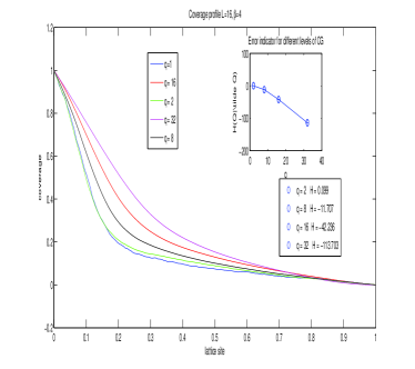
(a)   Stationary concentration profiles for different cell sizes $q$ with mean-field interactions. The inset depicts errors at different $q$ estimated by $\mathcal{H}$

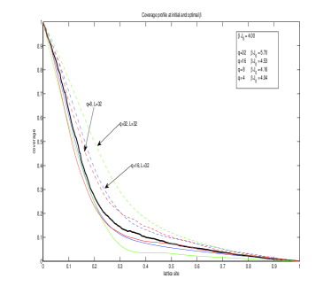
(b)   Stationary concentration profiles with fitted $\bar{J}(k;\theta^{*})$.

Figure 1: Coarse-grained simulations of driven diffusion of interacting particles without (a) and with (b) fitted effective interactions.

Next we discuss the parametric family of coarse-grained models we will use. Under the assumption of a local equilibrium a straightforward local averaging yields the coarse-grained rates, Katsoulakis and Vlachos (2003),

$$\bar{c}(k,l,\eta)=\frac{1}{q}\eta(k)(q-\eta(l))d\,e^{-\beta\bar{U}(k,\eta)}\,,$$ (36)

for the lattice-gas model with local concentrations $\eta(k)$ defined as the number of particles in a coarse cell $C_{k}$ of (lattice) size $q$. Thus we have $M$ coarse cells, where $N=qM$. In fact, according to (1) we define the coarse graining operator

$$\eta(k)=\mathbf{T}\sigma(k)=\sum_{x\in C_{k}}\sigma(x)\,,$$ (37)

where $\eta(k)\in\{0,\dots,q\}$. Keeping the two-body interactions as a basis for the coarse-grained approximation the effective potentials between block spins $k$ and $l$ are obtained by a straightforward spatial averaging

$$\bar{J}(k,l) =\frac{1}{q^{2}}\sum_{x\in C_{k}}\sum_{y\in C_{l}}J(x-y)\,,$$ (38)

$$\bar{J}(k,k) =\frac{1}{q(q-1)}\sum_{x\in C_{k}}\sum_{y\in C_{k}}J(x-y)\,.$$

Assuming that the approximating dynamics is of Arrhenius type we obtain the energy barriers

$$\bar{U}(k,\eta)=\sum_{l}\bar{J}(k,l)\eta(k)+\bar{J}(0,0)(\eta(k)-1)-\bar{h}\,.$$

The resulting dynamics is a Markovian approximation of the coarse-grained evolution and it is defined as CTMC with the rates $\bar{c}(k,l,\eta)$.

As a prototype example of the interactions we consider the constant potential $J(x)=J_{0}$ for $|x|\leq L$ and $J(x)=0$ otherwise. This coarse-grained potential is parametrized by a single parameter $\theta\equiv\bar{J}_{0}$ corresponding to the strength of the coarse-grained interactions.

First we note that he local mean-field approximation which defines the interaction potential $\bar{J}(k-l)$ in (38) between two block spins $\eta(k)$ and $\eta(l)$ by averaging contributions from all spin-spin interactions in the cells does not provide a good approximation as demonstrated in Figure 1(a), where the inset depicts the error estimated in terms of the entropy rate $\mathcal{H}({P}{\,|\,}{\tilde{P}})$. However, the mean-field potential $\bar{J}$ is a good initial datum for (18).

In this benchmark we stay in the family of two-body potentials and chose to fit only a single parameter that defines the total strength of the interaction. Thus the rates are parametrized by the effective potential $\bar{J}(\cdot;\theta)$ using the single parameter $\theta\equiv\bar{J}_{0}$, keeping the interaction range $L$ fixed in each set of simulations. Clearly we could consider much richer families with parametrized potentials, e.g., of Morse or Lennard-Jones type, however, we opt for the simplest parametrizations in order to demonstrate with clarity the proposed methods. The best-fit was obtained by solving the optimization problem (31), hence, minimizing the error defined by $\mathcal{H}({P}{\,|\,}{\tilde{P}^{\theta}})$, see Figure 2(a) and Figure 2(b). Figure 1(b) depicts concentration profiles for different sizes $q$ of the coarse cells. The dashed lines represent results from simulations with mean-field interactions between cells only (i.e., the initial guess in the optimization), while the solid lines represent simulations with the parametrized effective interactions.

Comparison with the profile obtained from the microscopic simulation (the solid black line) clearly indicates that when the coarse-graining size $q$ becomes close to the interaction range $L$ of the microscopic potential $J$ the best-fit in a one-parameter family is not sufficient for obtaining good approximation and a better candidate class of models, in this case coarse-grained (CG) dynamics $\bar{c}(k,l,\eta)$, needs to be found for improved parametrization. Indeed, in Are et al. (2008); Katsoulakis et al. (2013) we showed that coarse grained, multi-body cluster Hamiltonians provide such a parametrization. More specifically, in Katsoulakis et al. (2013) we demonstrated, through rigorous cluster expansions that (typical in the state-of-the-art) two-body CG approximations break down in lower temperatures and/or for short range particle-particle interactions, and additional multi-body CG terms need to be included in the models in order the CG model to capture accurately phase transitions and other physical important properties. Hence, a specific parametrization cannot consistently address this issue on its own, unless the proper classes of parametric models are first identified. The RER computations such as the one depicted in Figure 2(b) can assess the accuracy of different coarse-grained dynamics within the same parametric family (shown here), as well as determine the comparative coarse-graining accuracy of different parametric families.

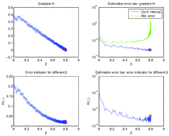
(a)   Convergence of the estimator $\hat{\theta}_{n}$ to the optimal value $\theta^{*}$.

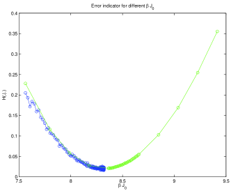
(b)   Dependence of $\mathcal{H}$ on the parameter $\theta$.

Figure 2: Minimization of $\mathcal{H}$. The figure (a) depicts convergence of the estimators for $\hat{\theta}_{n}$ and the gradient (derivative) $\nabla_{\theta}\mathcal{H}$ to the optimal value $\theta^{*}$ and the optimality condition $\nabla_{\theta}\mathcal{H}(\theta^{*})=0$. The right plots depict convergence of confidence intervals for the estimators. The figure (b) demonstrates the convexity of $\mathcal{H}$ with respect to $\theta$ which holds due to the particular choice $\theta\equiv\beta\bar{J}_{0}$ in the benchmark.

Example II: Two-scale diffusion process and averaging principle. In the second example we demonstrate the parametric approximation of the coarse-grained process on a system of two stochastic differential equations with slow and fast time scales

$$dX^{\epsilon}_{t}=a(X^{\epsilon},Y^{\epsilon})dt+dW^{1}_{t}$$ (39)

$$dY^{\epsilon}_{t}=\epsilon^{-1}b(X^{\epsilon},Y^{\epsilon})dt+\epsilon^{-1/2}dW^{2}_{t}\,,$$ (40)

where $W^{1}_{t}$, $W^{2}_{t}$ are independent standard Wiener processes. Under suitable assumptions on $a$, $b$ (see E, Liu, and Vanden-Eijnden (2005); Freidlin and Wentzell (2012)) the dynamics $Y^{\epsilon}_{t}$ with $x$ held fixed has a unique invariant measure $\mu^{\epsilon}_{x}(dy)$ and as $\epsilon\to 0$ we have the effective dynamics for the process $\bar{X}_{t}$ given by

$$d\bar{X}_{t}=\bar{a}(\bar{X}_{t})+dW_{t}\,.$$ (41)

The drift $\bar{a}$ is given by the averaging principle

$$\bar{a}(x)=\lim_{\epsilon\to 0}\int a(x,y)\,\mu_{x}^{\epsilon}(dy)\,.$$

In this example we choose the component $x$ as the coarse variable and compute an approximation of the drift $\bar{a}^{\epsilon}(x)$ for the coarse-grained (projected) process $X^{\epsilon}_{t}$. The averaging principle suggests that $\bar{a}^{\epsilon}\to\bar{a}$ as $\epsilon\to 0$.

For the specific choice

$$a(x,y)=-y\,,\;\;\mbox{and}\;\;\;b(x,y)=y-x\,,$$

we have that $\mu_{x}^{\epsilon}(dy)=\frac{1}{Z}\exp(-\frac{1}{2}(y-x)^{2})dy$ where $Z$ is the normalizing constant and thus $\bar{a}(x)=-\frac{1}{Z}\int y\exp(-\frac{1}{2}(y-x)^{2})dy=-x$ which yields the effective dynamics in the limit $\epsilon\to 0$. In the computational benchmarks we thus compare stationary processes resulting as $t\to\infty$ in solving

$$dX^{\epsilon}_{t}=-Y^{\epsilon}_{t}dt+dW^{1}_{t}\,,\;\;\mbox{the two-scale model,}$$ (42)

$$dY^{\epsilon}_{t}=\epsilon^{-1}(Y^{\epsilon}_{t}-X^{\epsilon}_{t})dt+\epsilon^{-1/2}dW^{2}_{t}\,,$$

$$d\bar{X}^{\epsilon}_{t}=-\sum_{k=1}^{K}\theta_{k}\phi(\bar{X}^{\epsilon}_{t})\,dt+dW_{t}\,,\;\;\mbox{CG model,}$$ (43)

$$d\bar{X}_{t}=-\bar{X}_{t}dt+dW_{t}\,,\;\;\mbox{asymptotic at $\epsilon\to 0$.}$$ (44)

The proposed method for approximating the coarse-grained dynamics constructs an effective potential $\bar{a}^{\epsilon}(x)=\sum_{k}\theta_{k}\phi_{k}(x)$ for a finite value $\epsilon>0$. The set of interpolating polynomials has been chosen to be $\{1,x,x^{2},x^{3},x^{4}\}$ in this example. It is expected that as $\epsilon\to 0$, the approximation $\bar{a}^{\epsilon}$ approaches the averaged coefficient $\bar{a}(x)=-x$.

The simulation results depicted in Figure 3 demonstrate that in the case of sufficient time-scale separation, $\epsilon=0.005$, the coarse-grained model well approximates the invariant distribution as well as the autocorrelation function for stationary dynamics of the component $X_{t}$. Furthermore, the drift $\bar{a}^{\epsilon}(x)$ of the coarse-grained dynamics deviates by a small error (see Figure 5) from the drift $\bar{a}(x)$ of the averaged model. On the other hand, for a larger value $\epsilon=0.5$, where the averaging principle does not apply, the proposed method yields a coarse-grained model (an “effective dynamics”) which still approximates reasonably well the invariant distribution. However, the dynamics of the stationary process $\bar{X}^{\epsilon}_{t}$ does not approximate properly the stationary behaviour of the slow component $X^{\epsilon}_{t}$ of the original process, as demonstrated in Figure 4 by comparison of autocorrelation functions.

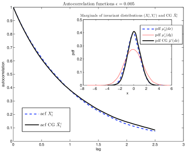
Figure 3: Autocorrelation function of the coarse-grained stationary process $\bar{X}^{\epsilon}_{t}$ solving (44) for $\epsilon=0.005$ and the autocorrelation function of the process $X^{\epsilon}_{t}$ solving (42). The inset depicts the invariant distribution for $\bar{X}^{\epsilon}_{t}$ and marginals of the invariant distribution of $X^{\epsilon}_{t},Y^{\epsilon}_{t}$.

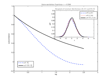
Figure 4: Autocorrelation function of the coarse-grained stationary process $\bar{X}^{\epsilon}_{t}$ solving (44) for $\epsilon=0.5$ and the autocorrelation function of the process $X^{\epsilon}_{t}$ solving (42). The inset depicts the invariant distribution for $\bar{X}^{\epsilon}_{t}$ and marginals of the invariant distribution of $X^{\epsilon}_{t},Y^{\epsilon}_{t}$.

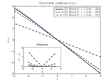
Figure 5: Comparison of fitted coefficients $\bar{a}^{\epsilon}(x)$ in the coarse-grained model (44) for different values of $\epsilon$ with the averaged drift $\bar{a}(x)$ in the asymptotic model (43).

Remark V.1.

The fact that the approximating coarse-grained process $\bar{X}^{\epsilon}_{t}$ is asymptotically close to the process $\bar{X}_{t}$ resulting from the averaging principle is a natural consequence of the proposed fitting method. We give here only a brief heuristic justification: the invariant distribution of the system (39) is $\mu^{\epsilon}(dx\,dy)=\bar{\mu}^{\epsilon}(dx)\mu(dy|x)$ where $\bar{\mu}^{\epsilon}$ is the (unknown) stationary distribution of a hidden effective dynamics. Under the assumption $\epsilon\ll 1$ we have $\mu^{\epsilon}(dx\,dy)\approx\bar{\mu}(dx)\mu_{x}(dy)$ where $\mu_{x}(dy)$ is the invariant distribution of the process $Y^{\epsilon}_{t}$ for fixed $x$. Thus the optimization problem (27) becomes for $\epsilon\to 0$

$$\min_{\bar{a}}\int|a(x,y)-\bar{a}(x)|^{2}\mu_{x}(dy)\bar{\mu}(x)\,dx\,,$$ (45)

which has the unique minimizer

$$\bar{a}(x)=\int a(x,y)\mu_{x}(dy)\,.$$ (46)

VI Conclusions

We developed parametrized model reduction methods with controlled-fidelity for the efficient and reliable coarse-graining of non-equilibrium molecular systems. Such systems are commonplace across all molecular and multi-physics models and arise as the result of coupling between different physical mechanisms, scales, external forcing, and boundary conditions. The methodology is based on concepts from path space information theory such as the Relative Entropy Rate (RER) and allows for constructing optimal parametrized Markovian coarse-grained dynamics within a given parametric family. The identification of the optimal parameters is achieved by minimizing information loss–due to coarse-graining–on the path space. Furthermore, a path-space analogue of the Fisher Information Matrix can be derived from RER and provides confidence intervals for the corresponding parameter estimators. We demonstrate the proposed coarse-graining methods in (a) non-equilibrium systems with diffusing interacting particles, driven by out-of-equilibrium boundary conditions, and (b) multi-scale diffusions and their corresponding stochastic averaging limits, and show that the proposed RER-based methodology can assess and improve the accuracy of different coarse-grained dynamics within the same parametric family. Finally, we expect that by employing systematically derived, e.g., via cluster expansions, Are et al. (2008); Katsoulakis et al. (2013), classes of parametric families of models, we can systematically assess accuracy vs. computational cost of more complex coarse-grained models, e.g., by including computationally costly multi-body interactions. The latter issue will be addressed in upcoming work.

Appendix A Microscopic reconstruction

In this Appendix we discuss the reconstruction procedure in (3). Reversing the coarse-graining, i.e., reproducing microscopic (fine-scale) properties, directly from coarse-grained (CG) simulations is an issue that arises extensively in the coarse-graining literature, e.g., Müller-Plathe (2002). The principal idea is that computationally inexpensive CG simulations will reproduce the large-scale structure and subsequently microscopic information will be added through microscopic reconstruction. Current approaches address primarily the equilibrium case and rely on conditioning on CG variables and subsequently carrying out a local equilibrium relaxation of the microscopic system.

We next provide a general mathematical framework for the reconstruction of fine-scale distributions or transition probabilities (3), from coarse-scale models. For concreteness we focus on reconstructing a fine-scale probability measure ${\mu}_{N}(d\sigma)$ defined on the fine-grained configuration space $\Sigma$, from a CG probability measure $\bar{\mu}_{M}^{\rm app}(d\eta)$ defined on the coarse space $\bar{\Sigma}$.

First we define

$$\bar{\mu}_{M}(d\eta)=\int_{\{\sigma:\mathbf{T}\sigma=\eta\}}{\mu}_{N}(d\sigma)$$

as the exact coarse-grained measure defined also in (2). Then, through the relation

$${\mu}_{N}(d\sigma)\equiv\,\mu_{N}(d\sigma|\eta)\bar{\mu}_{M}(d\eta)\,,$$ (47)

we define the conditional probability $\mu_{N}(d\sigma|\eta)$. In the sense of (2), we can view $\mu_{N}(d\sigma|\eta)$ as the (perfect) reconstruction of $\mu_{N}(d\sigma)$ from the exactly CG measure $\bar{\mu}_{M}(d\eta)$ defined in (2). Although many fine-scale configurations $\sigma$ correspond to a single CG configuration $\eta$, the “reconstructed” conditional probability measure $\mu_{N}(d\sigma|\eta)$ is uniquely defined, given the microscopic and the coarse-grained measures $\mu_{N}(d\sigma)$ and $\bar{\mu}_{M}(d\eta)$ respectively.

A coarse-graining scheme provides an approximation $\bar{\mu}_{M}^{\rm app}(d\eta)$ for $\bar{\mu}_{M}(d\eta)$. The approximation $\bar{\mu}_{M}^{\rm app}(d\eta)$ could be, for instance, the schemes discussed in Section V. To provide a reconstruction we need to lift the measure $\bar{\mu}_{M}^{\rm app}(d\eta)$ to a measure $\mu_{N}^{\rm app}(d\sigma)$ on the microscopic configurations. That is, we need to specify a conditional probability $\nu_{N}(d\sigma|\eta)$ and set

$$\mu_{N}^{\rm app}(d\sigma)\,:=\,\nu_{N}(d\sigma|\eta)\bar{\mu}_{M}^{\rm app}(d\eta)\,.$$ (48)

In the spirit of our earlier discussion on using relative entropy to quantify the quality of approximation in CG schemes, it is natural to measure the efficiency of the reconstruction by the specific relative entropy ${\cal R}\left(\mu_{N}^{\rm app}|{\mu}_{N}\right)$. A simple computationCover and Thomas (1991) shows that

$${\cal R}\left(\mu_{N}^{\rm app}{\,|\,}{\mu}_{N}\right)\,=\,{\cal R}\left(\bar{\mu}_{M}^{\rm app}{\,|\,}\bar{\mu}_{M}\right)+\int{\cal R}\left(\nu_{N}(\cdot|\eta){\,|\,}\mu_{N}(\cdot{\,|\,}\eta)\right)\bar{\mu}_{M}^{\rm app}(d\eta)\,,$$ (49)

i.e., relative entropy splits the total error at the microscopic level into the sum of the error at the coarse level and the error made during the reconstruction.

The first term in (49) can be controlled, for example, by error analysis results on the coarse variablesKatsoulakis et al. (2007, 2013). In order to obtain a suitable reconstruction we then need to construct $\nu_{N}(d\sigma\,|\,\eta)$ such that (a) it is easily computable and implementable, and (b) the error ${\cal R}\left(\nu_{N}(d\sigma\,|\,\eta){\,|\,}\mu_{N}(d\sigma{\,|\,}\eta)\right)$ should be of the same order as the first term in (49).

Example: The simplest example of reconstruction for a microscopic system $\mu(d\sigma)$ with a coarse-grained probability distribution $\bar{\mu}_{M}^{\rm app}(d\eta)$ is obtained by

$$\mu^{\rm app}(\sigma)\,:=\,U(\sigma|\eta)\bar{\mu}^{\rm app}(\eta)\,,$$ (50)

where $U(\sigma^{\prime}|\eta^{\prime})={1\over|\{\sigma:\mathbf{T}\sigma=\eta^{\prime}\}|}$ is the uniform conditional distribution over all fine-scale states $\sigma$ corresponding to the same coarse-grained state $\eta^{\prime}$. i.e., we first sample the CG variables $\eta$ using the CG probability; then we reconstruct the microscopic configuration $\sigma$ by distributing the particles uniformly on the coarse cell, conditioned on the value of $\eta$. More accurate, but computationally more demanding schemes were proposed in Trashorras and Tsagkarogiannis (2010); Kalligiannaki et al. (2012).

References

- Are et al. (2008) Are, S., Katsoulakis, M. A., Plecháč, P., and Rey-Bellet, L., SIAM J. Sci. Comput. 31, 987 (2008).
- Arnst and Ghanem (2008) Arnst, M. and Ghanem, R., Comp. methods in applied mech. and eng. 197, 3584 (2008).
- Bilionis and Zabaras (2012) Bilionis, I. and Zabaras, N., “A stochastic optimization approach to coarse-graining using a relative-entropy framework,” Tech. Rep. (Cornell University, 2012).
- Bonetto, Lebowitz, and Rey-Bellet (2000) Bonetto, F., Lebowitz, J. L., and Rey-Bellet, L., in Mathematical physics 2000 (Imp. Coll. Press, London, 2000) pp. 128–150.
- Bowman, Ensign, and Pande (2010) Bowman, G. R., Ensign, D. L., and Pande, V. S., Journal of Chemical Theory and Computation 6, 787 (2010).
- Carmichael and Shell (2012) Carmichael, S. P. and Shell, M. S., J. Phys. Chem. B 116, 8383 (2012).
- Chaimovich and Shell (2011) Chaimovich, A. and Shell, M. S., 134, 094112 (2011).
- Cover and Thomas (1991) Cover, T. and Thomas, J., Elements of Information Theory (John Wiley & Sons, 1991).
- Crowder (1976) Crowder, M. J., J. of the Royal Stat. Soc. Ser. B 38, 45 (1976).
- Dai, Seider, and Sinno (2008) Dai, J., Seider, W. D., and Sinno, T., The Journal of Chemical Physics 128, 194705 (2008).
- E, Liu, and Vanden-Eijnden (2005) E, W., Liu, D., and Vanden-Eijnden, E., Comm. Pure Appl. Math. 6, 1544 (2005).
- Eckmann, Pillet, and Rey-Bellet (1999) Eckmann, J.-P., Pillet, C.-A., and Rey-Bellet, L., Comm. Math. Phys. 201, 657 (1999).
- Espanol and Zuniga (2011) Espanol, P. and Zuniga, I., Phys. Chem. and Chem. Phys. 13, 10538 (2011).
- Freidlin and Wentzell (2012) Freidlin, M. I. and Wentzell, A. D., Random Perturbations of Dynamical Systems, 3rd ed. (Springer, 2012).
- Gillespie (1976) Gillespie, D. T., J. of Comp. Phys. 22, 403 (1976).
- Izvekov and Voth (2005a) Izvekov, S. and Voth, G. A., J. Phys. Chem. B 109, 2469 (2005a).
- Izvekov and Voth (2005b) Izvekov, S. and Voth, G. A., J. Chem. Phys. 123, 134105 (2005b).
- Jakšić, Pillet, and Rey-Bellet (2011) Jakšić, V., Pillet, C.-A., and Rey-Bellet, L., Nonlinearity 24, 699 (2011).
- Kalligiannaki et al. (2012) Kalligiannaki, E., Katsoulakis, M. A., Plechac, P., and Vlachos, D. G., J. Comp. Physics 231, 2599 (2012).
- Katsoulakis et al. (2007) Katsoulakis, M., Plecháč, P., Rey-Bellet, L., and Tsagkarogiannis, D., ESAIM: Math Model. Num. Anal. 41, 627 (2007).
- Katsoulakis, Majda, and Vlachos (2003) Katsoulakis, M. A., Majda, A., and Vlachos, D., Proc. Natl. Acad. Sci 100, 782 (2003).
- Katsoulakis et al. (2008) Katsoulakis, M. A., Rey-Bellet, L., Plecháč, P., and K.Tsagkarogiannis, D., J. Non Newt. Fluid Mech. (2008).
- Katsoulakis et al. (2013) Katsoulakis, M. A., Rey-Bellet, L., Plecháč, P., and Tsagkarogiannis, D. K., Math. Comp. (2013).
- Katsoulakis and Trashorras (2006) Katsoulakis, M. A. and Trashorras, J., J. Stat. Phys. 122, 115 (2006).
- Katsoulakis and Vlachos (2003) Katsoulakis, M. A. and Vlachos, D. G., Journal of Chemical Physics 119, 9412 (2003).
- Kipnis and Landim (1999) Kipnis, C. and Landim, C., Scaling Limits of Interacting Particle Systems (Springer-Verlag, 1999).
- Lyubartsev et al. (2003) Lyubartsev, A. P., Karttunen, M., Vattulainen, P., and Laaksonen, A., Soft Materials 1, 121 (2003).
- Majda and Gershgorin (2010) Majda, A. J. and Gershgorin, B., Proc. of the National Academy of Sciences 107, 14958 (2010).
- Majda and Gershgorin (2011) Majda, A. J. and Gershgorin, B., Proc. of the National Academy of Sciences 108, 10044 (2011).
- Müller-Plathe (2002) Müller-Plathe, F., Chem. Phys. Chem. 3, 754 (2002).
- Noid et al. (2008) Noid, W. G., Chu, J. W., Ayton, G. S., Krishna, V., Izvekov, S., Voth, G. A., Das, A., and Andersen, H. C., J. Chem. Phys. 128, 244114 (2008).
- Padding and Briels (2011) Padding, J. T. and Briels, W. J., Journal of Physics: Condensed Matter 23, 233101 (2011).
- Pantazis and Katsoulakis (2013) Pantazis, Y. and Katsoulakis, M., J. Chem. Phys. 138, 054115 (2013).
- Rey-Bellet and Thomas (2002) Rey-Bellet, L. and Thomas, L. E., Comm. Math. Phys. 225, 305 (2002).
- Smit and Maesen (2008) Smit, B. and Maesen, T. L. M., Chem. Reviews 108, 4125 (2008).
- Stamatakis and Vlachos (2012) Stamatakis, M. and Vlachos, D. G., ACS Catalysis 2, 2648 (2012).
- Trashorras and Tsagkarogiannis (2010) Trashorras, J. and Tsagkarogiannis, D. K., SIAM Journal on Numerical Analysis 48, 1647 (2010).
- Tschöp et al. (1998) Tschöp, W., Kremer, K., Hahn, O., Batoulis, J., and Bürger, T., Acta Polym. 49, 61 (1998).
- Vlachos and Katsoulakis (2000) Vlachos, D. G. and Katsoulakis, M. A., Phys. Rev. Lett. 85, 3898 (2000).