The XMM Deep survey in the CDFS V. Iron K lines from active galactic nuclei in the distant Universe

Abstract

Context. X-ray spectroscopy of active galactic nuclei (AGN) offers the opportunity to directly probe the inner regions of the accretion disk. Reflection of the primary continuum on the circumnuclear accreting matter produces features in the X-ray spectrum that help to explore the physics and the geometry of the innermost region, close to the central black hole.

Aims. We present the results of our analysis of average AGN XMM-Newton X-ray spectra in the Chandra Deep Field South observation (hereafter, XMM CDFS), in order to explore the Fe line features in distant AGN up to z$\sim$3.5.

Methods. We computed the average X-ray spectrum of a sample of 54 AGN with spectroscopic redshifts and signal-to-noise ratio in the 2-12 keV rest-frame band larger than 15 in at least one EPIC camera (for a total of 100 X-ray spectra and 181623 net counts in the 2-12 keV rest-frame band). We have taken the effects of combining spectra from sources at different redshifts and from both EPIC-pn and EPIC-MOS cameras into account, as well as their spectral resolution; we checked our results using thorough simulations. We explored the iron line components of distant AGN focusing on the narrow core which arises from material far from the central BH and on the putative relativistic component emitted in the accretion disk.

Results. The average spectrum shows a highly significant iron feature. Estimating its equivalent width (EW) with a model-independent method suggests a higher EW in a broader range. The line, modelled as an unresolved Gaussian, is significant at 6.8$\sigma$ and has an EW=$95\pm 22$ eV for the full sample. We find that our current data can be fitted equally well adding a relativistic profile to the narrow component (in the full sample, EW=$140\pm 120$ eV and 67$\pm 28$ eV respectively for the relativistic and narrow lines).

Conclusions. Thanks to the high quality of the XMM CDFS spectra and to the detailed modelling of the continuum and instrumental effects, we have shown that the most distant AGN exhibit a highly significant iron emission feature. It can be modelled both with narrow and broad lines which suggest that the EW becomes higher when a broader energy range around the line centroid is considered, provides tantalising evidence for reflection by material both very close and far away from the central engine. The EW of both features are similar to those observed in individual nearby AGN, hence they must be a widespread characteristic of AGN, since otherwise the average values would be smaller than observed.

1 Introduction

X-ray spectroscopy of active galactic nuclei (AGN) provides one of the most useful probes of the properties of the accretion disks in the vicinity of the super massive black holes (SMBHs). In particular, the iron K_α line is widely used to study the SMBH relativistic effects, therefore giving unique information about the location and the kinematics of the accreting material. Relativistic effects produce a line deformation when fluorescence occurs in regions a few gravitational radii away from the central SMBH. Given that the inner radius of the accretion disk is 6$R_{g}$ around a non-rotating black hole (BH) and 1.23 $R_{g}$ ($R_{g}$=$\frac{GM}{c^{2}}$) if the BH is maximally rotating (Bardeen et al. 1972), the velocities involved approach the speed of light and, furthermore, the strong gravitational field of the BH itself will cause a gravitational redshift effect. Since the theoretical predictions on AGN relativistic lines (Fabian et al. 1989), such features have been found in the X-ray spectra of several Seyferts, being MGC-6-30-15 the best studied one (Tanaka et al. 1995).

A broad Fe K$\alpha$ line can be diluted in the continuum if the signal-to-noise ratio (S/N) is low (Guainazzi et al. 2006). This demonstrates the necessity of high S/N data with good counts statistics to detect the relativistic features in the iron lines, (Guainazzi et al. 2011; de la Calle Pérez et al. 2010; Nandra et al. 2007). Theoretical predictions (Ballantyne 2010) supported this scenario, showing that the majority of relativistic iron lines have equivalent widths (EW) of just 100 eV, highlighting the importance of high sensitivity surveys to explore them. In cases where the individual X-ray observations have a limited S/N, statistical methods like integrating or averaging the spectra can be used for their analysis. Nandra et al. (1997) used for the first time a statistical approach to study the ASCA X-ray spectra of an AGN survey: they found that a broad line is present not only in the majority of their Seyfert sample, but also in their average spectrum, with a shape similar to those of the individual source spectra probing therefore that these features are common in the low redshift universe. Their more recent work (Nandra et al. 2006) on an XMM-Newton broad line survey confirmed this result, finding that in 1/3 of their sample the iron lines are well described by the sum of a narrow line likely coming from reflection in distant cold matter in the inner edge of the torus, and a relativistic line coming from the accretion disk, much closer to the SMBH.

The deep observation with XMM-Newton of the Lockman Hole was studied with a statistical approach, showing a broad stacked iron line, with a relativistic shape (Streblyanska et al. 2005). Some further tantalising evidence for a broad iron line was also found in Brusa et al. (2005) and Civano et al. (2005): they computed the stacked X-ray spectra of the Chandra Deep Fields, cautioning that their large EW and broad profile significantly depend on the modelling of the underlying continuum. In fact, the EW of the lines found in these early works were much higher (of the order of many 100 eV) than those found in local individual AGN, which casted some doubts on their reality.

Unlike these first spectroscopic studies of the AGN surveys with stacking, many recent papers have successfully detected narrow iron lines, while the broad lines are not clearly seen. Examples of such detections include the XMM-Newton X-ray observations of the AXIS (Carrera et al. 2007) and XWAS samples studied by Corral et al. (2008) and the subsample with 0.2-12 keV counts greater than 1000 of the 2XMM X-ray source catalogue (Watson et al. 2008) studied by Chaudhary et al. (2010, 2012). Therefore, the detection of broad Fe lines in stacked spectra of distant AGN remains controversial.

More recently, Iwasawa et al. (2012) found evidence for ionised iron lines in the stacked spectrum of the COSMOS sample. Broad symmetrical lines were found in the low luminosity - low redshift AGN in the deep Chandra Fields (Falocco et al. 2012). Taking the COSMOS results into account, such symmetrically broadened lines were interpreted as the combination of a relativistic profile and several narrow lines centred at 6.4 keV and higher energies, from iron at a variety of ionisation states. Consequently the total iron line emission will appear symmetrically smoothed (Falocco et al. 2012).
In this paper, we present the result of an X-ray spectral analysis of the deepest XMM-Newton survey made so far: the 3 Ms observation centred in the Chandra Deep Field South (Comastri et al. 2011). This survey enables a much more detailed spectroscopic study than earlier data on this or other deep surveys and allows us to study the accretion at the epoch of the peak of the activity in the history of galaxy evolution at z$\sim$1-2 (Ueda et al. 2003; Ebrero et al. 2009). It covers three orders of magnitude in luminosity ($10^{41.5}-10^{44.5}\rm erg$ $\rm s^{-1}$), which allows us to study the behaviour of the spectral features coming from the accretion disk in X-rays, and the trend found between the Fe line EW with the luminosity (Iwasawa & Taniguchi 1993).

The paper is organised as follows. The properties of the sample are described in Sect. 2, the method used to average the spectra in Sect. 3; our results are illustrated in Sect. 4; and in Sect. 5 we discuss the implications, summarising our conclusions in Sect. 6. Throughout this paper, we adopt the cosmological parameters: $H_{\ 0}$=70 km s^-1 Mpc^-1, $\Omega_{matter}$=0.3 and $\Omega_{\Lambda}$=0.7; all the counts refer to the net number of counts between 2 and 12 keV rest-frame, unless explicitly stated otherwise. We used xspec v. 12.5 (Arnaud 1996) for the X-ray spectral analysis; the error estimates correspond to 90% confidence level for one interesting parameter.

2 X-ray sample

We present in this section the XMM-Newton observation in the CDFS and its spectral analysis in 2.1, the definition of the 54 sources sample in 2.2, and the definition of the various subsamples in 2.3.

Table 1: Properties of the full sample with S/N$>15$ and its subsamples

Sample	$N_{sp}$	Ns	$N_{2-12}$	$N_{5-8}$	$\langle z\rangle$	$\langle\log(L)\rangle$	$\langle N_{\rm H,22}\rangle$	$N_{\rm H,22}$	$\langle S/N\rangle$	$\alpha$	$\Sigma_{6}$
						(erg s-1)	($10^{22}$ cm-2)	($10^{22}$ cm-2)			(eV)
(1)	(2)	(3)	(4)	(5)	(6)	(7)	(8)	(9)	(10)	(11)	(12)
Full	100	54	181623	40863	1.34	43.74	1.48	0.08	29.8	0.35	119
Unabs	52	32	110523	21071	1.27	43.78	0.02	0.0	33.60	0.34	122
Abs	29	17	45896	14373	1.28	43.64	4.90	2.41	24.88	0.37	116
z$<1$	39	20	72672	18148	0.64	43.21	1.61	0.17	30.0	0.35	95
z$\geq 1$	61	34	108951	22715	1.80	44.07	1.39	0.04	28.8	0.35	134
Sey	61	33	91511	20987	0.91	43.35	1.35	0.11	26.2	0.34	108
QSO	39	21	90111	19876	2.02	44.34	1.68	0.04	34.1	0.36	138

2.1 The X-ray data

The XMM CDFS survey is an observation of the Chandra Deep Field South with XMM-Newton for a total of 3.3 Ms of full exposure time. Exposure times from the EPIC pn and MOS cameras are 2.5 Ms and 2.8 Ms respectively. The bulk of the observations were performed between July 2008 and March 2010, and have been combined with archival data taken between July 2001 and January 2002. The details on data reduction and analysis and the source detection algorithm are presented in Ranalli et al. (2013).

In this work, we used the high quality X-ray spectra for sources detected with a significance above 8 sigma in the 2-10 keV source catalogue, corresponding to a flux limit of $\sim$ 2 $\times$ $10^{-15}$erg s^-1cm^-2.

We looked for spectroscopic identifications of these sources in the literature making use of several spectroscopic campaigns (Le Fèvre et al. 2004; Szokoly et al. 2004; Le Fèvre et al. 2005; Mignoli et al. 2005; Ravikumar et al. 2007; Kriek et al. 2008; Vanzella et al. 2008; Taylor et al. 2009; Treister et al. 2009; van der Wel et al. 2005; Balestra et al. 2010; Silverman et al. 2010; Casey et al. 2011; Cooper et al. 2011). To avoid possible spurious broad line detections caused by errors in the redshift estimate, which could produce a false line broadening, we used only sources with spectroscopic redshifts defined as secure in the literature.

To characterise the spectra and to estimate their intrinsic luminosities, after grouping the XMM-Newton EPIC MOS and PN spectra at 20 counts per bin, the spectra were fitted with xspec using the $\chi^{2}$ statistics between 1 and 12 keV rest-frame in order to fit the broadest possible band avoiding the background-dominated E$>$12 keV rest-frame band (for this spectral region our grouping of 20 counts per bin would not probably be a suitable choice due to the background); we do not consider the soft X-ray band (E$<$1keV) due to the onset of complex spectral features (warm absorption and soft excess). We used a simple powerlaw modified by Galactic absorption, frozen at a column density $\sim 8\leavevmode\nobreak\ \times\leavevmode\nobreak\ 10^{19}\leavevmode\nobreak\$cm^-2 (Stark et al. 1992), and variable intrinsic absorption. We analysed the background spectrum and found an emission feature coincident with the position of the Al line characterising many background spectra at observed-frame energy $\sim$ 1.5 keV (Carter & Read 2007). However, this feature is not expected to influence significantly our iron line analysis, as there is only one object at z higher than 3.27, value which would shift the Al feature to 6.4 keV. To assess whether this systematic feature influences the output of our fits, we repeated the fits removing the channels corresponding to $1.5\pm 0.1$ keV. The fit results show that the presence of this background feature does not really influence the output fit parameters very much: comparing for example the intrinsic absorption estimated in X-rays, we found that the difference is negligible in the majority of the sample, with the exception of a handful of spectra (seven, for which we used the fit parameters obtained ignoring these channels). The luminosities were estimated from the best fit models of each spectrum, corrected for Galactic and intrinsic absorption, and calculated between 2 and 10 keV rest-frame. These are the luminosities used in the remainder of this paper for each spectrum. In the case of sources with both EPIC MOS and pn spectra, when a single value per source is presented (e.g. Fig. 3), we have used the value corresponding to the spectrum with the highest S/N.

In the remainder of the paper, the luminosities are always indicated in ${\rm erg}\,{\rm s}^{-1}$ and the intrinsic absorption will always be in units of cm^-2.

2.2 Sample definition and properties

It has been found empirically that a good S/N is essential for a significant detection of a broad line with the EPIC cameras (de la Calle Pérez et al. 2010; Guainazzi et al. 2011).

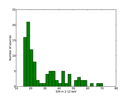
Figure 1: Spectral signal-to-noise-ratio between 2-12 keV of the full (100 spectra) sample.

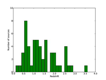
Figure 2: Redshift distribution of the full (54 X-ray sources) sample.

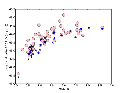
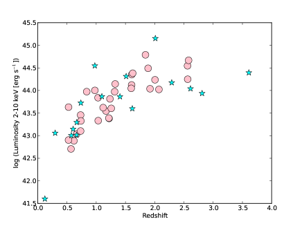
Figure 3: Top panel: Distribution in the Luminosity-redshift plane of the 54 XMM CDFS sources (pink circles) and of the 33 Chandra Deep Field South sources (blue stars) by Falocco et al. (2012). Bottom panel: Distribution in the Luminosity-redshift plane of the 17 absorbed (cyan stars) and 32 unabsorbed (pink circles) subsamples.

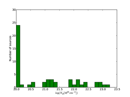
Figure 4: $\log{\left(N_{\rm H}\right)}$ distribution of the full sample. $N_{\rm H}$ is in units of $10^{22}$ cm^-2; all the values $\log{\left(N_{\rm H}\right)}<20$ have been replaced with $\log(N_{\rm H})=20$ for plotting purposes only.

To maximise the average S/N of the sample, taking the level of the background of the XMM-Newton observation into account, we limited our investigation to the 100 spectra corresponding to 54 unique sources (49 spectra from the EPIC-MOS cameras and 51 spectra from the EPIC-pn camera) characterised with S/N$>$15 estimated between 2 and 12 keV rest-frame (the band used in the analysis of the average spectra described below). This selection of the sample represents a compromise between the need to avoid including noisy sources and the necessity to have a high enough number of sources in the sample for good statistics. We discarded the two brightest sources whose number of counts (about 20000 net counts each) is significantly higher than those characterising the other sources (each of the sources analysed here have less than 10000 net counts in the 2-12 keV rest-frame band and the total accumulated counts by the 54 sources is about 180000). In this way we avoid the estimated average spectra being dominated by the two brightest sources, which would be contributing 10% of the total counts each. These sources are: PID 319 and PID 203 (Ranalli et al. 2013), the latter shows a remarkable and variable iron line.

The high quality of the spectra can be seen in the Fig. 1, where the distribution of the S/N (in 2-12 keV) of the 100 selected spectra is shown. We can see in Fig. 2 the distribution of the spectroscopic redshifts of the sources included in the sample: 21 AGN in our sample are located at redshifts z$\sim$1-2 and a dozen AGN at earlier epochs ($z\sim 2-3$). Note, from this distribution, that the rest-frame 2-12 keV band used in this paper, corresponds to an observed band of 1-6 keV at a typical z$\sim$1, therefore avoiding strong fluorescent signatures in the detectors’ background.

Figure 3 shows the distribution of the sample sources in the luminosity - redshift plane. In this figure, only one entry per physical source is presented: in sources where both the spectra from MOS and from pn are available, we display the result for the highest S/N spectrum. The CDFS observation by XMM-Newton allows a better coverage of the luminosity-redshift plane than our previous work on the Chandra spectra of the sources detected in the deep Chandra fields (see top panel of Fig. 3). The XMM CDFS survey is able to characterise with the highest significance reached so far the properties of distant X-ray selected AGN over three orders of magnitude of continuum luminosity and a broad span of redshifts, up to $\sim 3.6$. Despite the good counting statistics of the individual spectra, the kind of analysis of the iron line we carry out in this paper requires much higher statistics, hence we perform stacking.

2.3 Subsample definition

The sample characteristics and properties are listed in Table 1. We constructed two luminosity subsamples with similar number of counts in each, resulting in a Seyfert subsample with $\log{\left(L\right)}<44$ (hereafter, we call refer to this subsample as Sey) and a quasi stellar object (QSO) subsample with $\log{\left(L\right)}\geq 44$ (hereafter, we call this subsample QSO).

We also segregated the full sample in two redshift subsamples with the same number of counts. The low-z subsample includes all the sources with z $<$ 1. The high-z subsample includes all the sources with z$\geq 1$. We did not define more than two subsamples because we preferred to have as many source counts in each to attempt a sensitive assessment of the iron line trend with these parameters.

Finally, we separated the full sample in two subsamples of different intrinsic column density estimated in X-rays (’$N_{\rm H}$ subsamples’) setting the threshold at $\log{\left(N_{\rm H}\right)}=21.5$. This is often used as the threshold below which the interstellar medium of the galaxies hosting the AGN could provide the obscuration of broad lines in optical spectra (Caccianiga et al. 2007). The $N_{\rm H}$ distribution (see Fig. 4) extends from $\log{\left(N_{\rm H}\right)}<20$ to $\log{\left(N_{\rm H}\right)}\sim 23$. The $\rm N_{H}$ shown in the figure have been obtained from the fits to the individual spectra. For sources with both MOS and pn spectrum, we present the result from the best S/N spectrum. We can also appreciate in this Figure that around $\log{\left(N_{\rm H}\right)}\sim 21.5$ there is a clear gap between lower and higher absorption sources, making this value a ‘natural’ choice for our sample.

The two $N_{\rm H}$ subsamples have been constructed considering the errors $\Delta N_{\rm H}$ on the $N_{\rm H}$ obtained in the fits to the individual spectra. The sample, which includes the sources for which at 90 % of confidence $\log{\left(N_{\rm H}+\Delta N_{\rm H}\right)}<21.5$ (hereafter called ’Unabs’ subsample) accumulates about 111000 net counts in the 2-12 keV rest-frame band, while the sample with $\log{\left(N_{\rm H}-\Delta N_{\rm H}\right)}\geq 21.5$ at 90 % of confidence (called hereafter ’Abs’ subsample) contains about 46000 net counts in the same band. Nineteen spectra have not been included in the two above mentioned subsamples (i.e., the 90% error bars around the best fit $N_{\rm H}$ values cross the $\log{\left(N_{\rm H}\right)}=21.5$ borderline that separates ’Abs’ from ’Unabs’ sources). These unclassified spectra contain 25204 and 5419 counts respectively in the 2-12 keV and the 5-8 keV rest-frame bands.

We note that, despite its name, the ’Abs’ subsample consists mostly of moderately absorbed AGN (median $N_{\rm H}\sim 2.4\times 10^{22}\rm cm^{-2}$). Our sample does not contain any Compton thick sources, so we do not expect to detect in the average spectra of the absorbed sample any strong absorption feature in the iron line region. The two $N_{\rm H}$ subsamples are characterised by a similar distribution in the luminosity-redshift plane (see bottom panel of Fig. 3), allowing to assess whether the intrinsic absorption alone can influence the detection of the X-ray spectral features of the AGN. In the Fig. 3, one entry per each physical source is shown (if the spectra from both MOS and pn are available, we plot the best S/N spectrum). In the Fig. 3, the 54 XMM CDFS sources have higher luminosities at the same redshift range than the 33 Chandra CDFS AGN. According to the Iwasawa-Taniguchi effect, a higher luminosity corresponds to a lower iron line EW, thus the spectra from the XMM CDFS will not be particularly advantaged in the iron feature detection.

3 Analysis method

The averaging method used here was presented for the first time (Corral et al. 2008, 2011) in the study of XMM-Newton spectra of the XMS-XWAS surveys (Carrera et al. 2007; Mateos et al. 2008) and for the XBS survey (Della Ceca et al. 2004); later, it was adapted and tested for the deep Chandra Fields by Falocco et al. (2012). In this work we refined the technique of analysis introducing new methodologies that will be described in Sect. 3.3 and 4.1.

3.1 Averaging method

After fitting the spectra of every individual source as described in Sect. 2.1, we read into xspec again each unbinned, background-subtracted spectrum, and we used the corresponding best-fit (to the binned spectrum) model to extract the unfolded spectrum compensating for the effective area of the instrument (eufspec command in xspec). The unfolded spectra depend on the model used for this operation. In Falocco et al. (2012), we have checked the effect of the correction for detector response on the average spectrum, demonstrating the independence on the model used in the unfolding process above $\sim$2 keV, even for models clearly different from the input spectrum. Our simulations (as explained in Sects. 3.2 and 3.3) take any effect of the uncertainty in the continuum shape into account, since each simulated spectrum is fitted and the corresponding best fit model is used for the unfolding, instead of the input shape.

Once we obtained all the unfolded spectra, in analogy to what was done in Falocco et al. (2012) and in Corral et al. (2008), we applied the following procedure:

1. Correction for Galactic absorption,

2. Shift the spectra to rest-frame,

3. Re-normalise each spectrum by dividing by its integrated flux in the 2-5, 8-10 keV spectral range

We used the 2-10 keV rest-frame band in the last step (excluding the 5-8 keV rest-frame range were the putative iron line is expected to contribute most) to avoid giving too much weight to absorbed sources, which are in much higher proportion of the full sample with respect to our previous work in Falocco et al. (2012), where we used only the 2-5 keV rest-frame band for the normalisation.

To minimise the effect of the Al spike at 1.5 keV in the spectra from XMM CDFS (discussed in Sect. 2.1), we ignored the bins corresponding to rest-frame energy in the range 1.4-1.6 keV observed frame (compensating for the lost flux by interpolating linearly to the full band) when estimating the continuum for the normalisation and also in the final average of both the real and the simulated data.

We binned the spectra using an energy grid with 100 eV-wide bins and we finally averaged them. The errors were estimated as the dispersion of the fluxes around the average.

We have found that if we use instead error bars obtained from error propagation of the individual source bins, as we did in Falocco et al. (2012), the combined error bars were smaller, resulting in very high reduced $\chi^{2}$ values. We believe that this is because, with these new data with more net counts, the intrinsic spectral dispersion dominates over the counting noise.

3.2 Simulations of the continuum

We have estimated the expected shape of the underlying continuum in our spectra using comprehensive simulations.

We simulated the spectrum of each source 110 times using the best-fit parameters of the simple absorbed power law model from the individual fits to the real spectra (see Sect. 2.1). To each of these 110 simulated samples we applied the same method as the one used for the observed sample (spectral fitting, unfolding to correct for the instrument’s energy-dependent response, correcting for Galactic absorption, shift to rest-frame, normalising, averaging and calculation of errors from the dispersion). After this, we adopted as the underlying continuum the median of the simulated continua. The median is preferred over a simple average because it is a more robust estimate of the central value of a distribution.

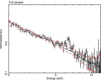
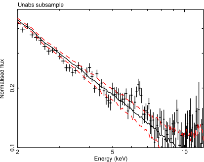
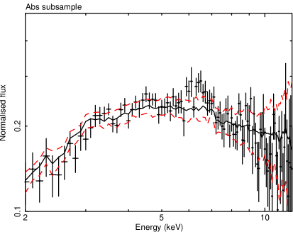
Figure 5: Average observed spectrum (data points) with its simulated continuum (continuous line) and the $1\sigma$ confidence levels of our simulations (dashed lines). From top to bottom: full sample, Unabs subsample, Abs subsample. The dotted line in the top panel represents the intrinsic resolution at 6.4 keV obtained from the simulations of the iron line described in Sect. 3.3.

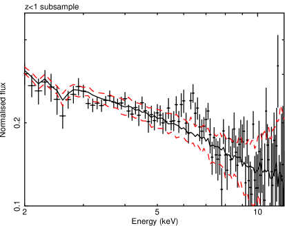
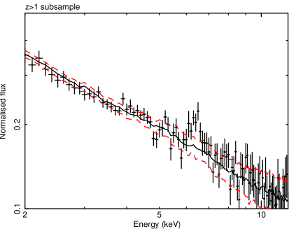
Figure 6: Average observed spectrum with its simulated continuum and the $1\sigma$ confidence lines. Top panel: z$<$1 subsample, bottom panel: z$\geq$1 subsample. Symbols and line styles as in Fig. 5.

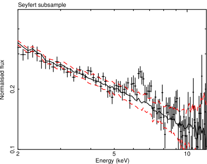
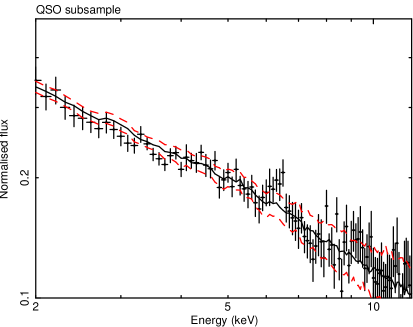
Figure 7: Average observed spectrum with its simulated continuum and the $1\sigma$ confidence lines. Top panel: Sey subsample, bottom panel: QSO subsample. Symbols and line styles as in Fig. 5.

We present in Figs. 5, 6, 7 our average spectra together with their corresponding simulated continua. In those figures we present: the average observed spectrum (data points), our simulated continuum (continuous line) and the $1\sigma$ confidence lines of our continuum simulations (dashed lines). The latter were estimated from the 68% percentiles around the median.

An intense iron line characterises the observed spectra of the sample and all the subsamples that we constructed. Its profile appears visually broader than the instrumental resolution, in the full sample (shown in the top panel of Fig. 5).

3.3 Simulations of the Fe Line

The spectral resolution of the X-ray detectors and the averaging process can widen any narrow spectral features in the X-ray spectra making them to appear artificially broader than they actually are. The resulting effective spectral dispersion changes with energy and, consequently, our ability to resolve spectral features will change along the spectrum. To properly study the iron line profile in the XMM CDFS, we need to estimate our effective spectral dispersion in the energy band we are analysing. To do this, we ran high S/N simulations of unresolved ($\sigma=0$) Gaussian emission lines centred at rest-frame energies between 1 and 10 keV, in steps of 1 keV with input EW of 200 eV (one simulation for each source -at its observed redshift-, and for each energy). The input continuum model was a powerlaw with $\Gamma=1.9$ without any intrinsic absorption. We corrected the spectra for detector response (modelling them with a powerlaw with photon index 1.9) as done in Corral et al. (2008) and Falocco et al. (2012); then we applied the same treatment described in Sect. 3. We then studied how the width of the simulated lines changes with the central energy. In addition, in analogy with what we did in Falocco et al. (2012), we simulated lines centred at 6.4 keV and 6.9 keV to estimate the resolution at the peak energy of the line from neutral and ionised iron. We recovered the input parameters of the continuum very well, reproducing a powerlaw continuum with $\Gamma\sim$1.9, while the Gaussian lines appear broadened by $\Sigma\sim$ 100 eV. A similar value of the spectral resolution given by the stacking procedure and the X-ray instruments was found in the study of the XMM-Newton X-ray spectra in the COSMOS sample (Iwasawa et al. 2012).

We studied the width of the average simulated lines as a function of their centroid energies: the result shows, for the full sample, $\Sigma=119\leavevmode\nobreak\ \rm eV\leavevmode\nobreak\ \left(\frac{E}{6\leavevmode\nobreak\ \rm keV}\right)^{0.34}$. The values of the $\Sigma$ obtained in this work include the contributions from the spectral dispersion of the instruments, $\Sigma\sim$ 55 eV (Haberl et al. 2002), as well as the widening introduced by the averaging method. The parameters of this $\Sigma(E)$ dependence (the slope and the $\Sigma$ at 6 keV) for the full sample and its subsamples are in Table 1. This energy-dependent instrumental response has been taken into account in the spectral fitting of the average spectra.

We emphasise that this limited spectral resolution essentially means that any features narrower than about 0.1 keV are very likely due to statistical fluctuations.

4 Results

We discuss in this section the results of our analysis of the average XMM-Newton X-ray spectra of several subsamples in the XMM CDFS, estimating in particular the iron line significance and shape. A new way to estimate the line EW independent of the fits to the average spectra has been applied and it is described in 4.1. We describe the detailed spectral fits to the data in the Sect. 4.2.

4.1 Model-independent estimate of the line EW

We compared the features found in our average observed spectrum with the average simulated spectra to estimate the line EW (see Table 2). To do this, we used the following energy ranges: 5.5-7 keV (that we call, for convention, bulk), 6-6.8 keV (called neutral), 6.2-6.6 keV (called narrow), 6.8-7 keV (called ionised), chosen to represent several spectral features from relativistically-broadened neutral Fe-K lines (5.5-7. keV), and from narrow neutral Fe lines (6.2-6.6 keV), to symmetrically broadened lines (6.0-6.8 keV) to lines from H-like Fe (6.8-7.0 keV), taking our spectral resolution ($\Sigma\sim 0.1$ keV) into account. We did not considered an interval centred at 6.7 keV to represent the line from He-like Fe because the average spectra do not visually display this feature (see Figs. 6-8).

We estimated the EW of the iron line using the 110 simulated continua and used the same energy bands described above. For each simulation we calculated the integral: EW=$\int_{E_{1}}^{E_{2}}dE\frac{T(E)-C(E)}{C(E)}\sim\sum\Delta(E_{i})\frac{T(E_{i})-C(E_{i})}{C(E_{i})}$ where $\Delta(E_{i})$ is the width of the bin with centre $E_{i}$; $T(E_{i})$ represents the average observed spectrum, $C(E_{i})$ the average continuum. The values of the median of the EW for each subsample and energy range are shown in Table 2. The confidence levels in that Table are calculated from the 68% percentiles around the corresponding medians.

There is evidence for a significant decrease of the EW of the narrow line with increasing average luminosity, in agreement with the ’Iwasawa-Taniguchi effect’ (Iwasawa & Taniguchi 1993). No significant trend with redshift has been found. The EW estimated in the ’bulk’ range is higher for the Unabs subsample than for the Abs subsample, as expected (because unabsorbed AGN are seen preferentially face-on), we should note that the N_H values covered by the absorbed sample that we defined in this work are too low to affect significantly the continuum above 6 keV, thus the iron line region. The same consideration should be applied to understand also the lower EW estimated in the ’neutral range’ for the Abs subsample, despite a higher EW of the narrow core expected when absorption is significant.

Table 2: Median of the EW calculated in different energy ranges using the simulations.

Energy band	Bulk	Neutral	Narrow	Ionised
sample	5.5-7.	6.0-6.8	6.2-6.6	6.8-7.
Full	$203_{-30}^{+33}$	$160_{-23}^{+21}$	$117_{-16}^{+14}$	$26_{-11}^{+15}$
Unabs	$252_{-38}^{+48}$	$194_{-38}^{+42}$	$156_{-26}^{+40}$	$38_{-24}^{+18}$
Abs	$192_{-26}^{+26}$	$150_{-30}^{+38}$	$86_{-46}^{+46}$	$18^{+16}_{-12}$
z$<$1	$254_{-53}^{+50}$	$166_{-34}^{+38}$	$119_{-29}^{+28}$	$37_{-18}^{+19}$
z$\geq$1	$176_{-47}^{+37}$	$160_{-31}^{+28}$	$118_{-22}^{+20}$	$21_{-17}^{+16}$
Sey	$283_{-48}^{+51}$	$213_{-37}^{+26}$	$148_{-21}^{+22}$	$47_{-20}^{+20}$
QSO	$71_{-29}^{+40}$	$87_{-25}^{+25}$	$66_{-15}^{+21}$	$<32$

4.2 Spectral fits to the full sample and subsamples

To characterise the spectral features of our average spectra and to understand their physical origin, we fitted them in the full rest-frame 2-12 keV band (ignoring the E$<$2 keV rest-frame band in this analysis because we are not interested here in studying the soft excess).

In our analysis of the deep Chandra fields of Falocco et al. (2012) the average simulated spectrum was employed as a continuum in the spectral fits. That approach does not take the uncertainty in the shape of the underlying continuum into account. In the current work, we preferred to construct an empirical continuum with a flexible, smooth shape. To take the instrumental line broadening discussed in Sect. 3.3 into account, we smoothed the input spectral model with a Gaussian convolution model (gsmooth in xspec). This model smooths the spectral features with a Gaussian with a variable sigma, which changes as a function of the energy (the powerlaw slope and the $\Sigma$ found in our simulations of the unresolved lines in Sect. 3.3 and summarised in Table 1 are used), hence, all the parameter values given below are ’intrinsic’ values, i.e., with the instrumental/method resolution already subtracted.

Our continuum is an absorbed powerlaw plus a Compton reflection component (both represented by a pexrav model in xspec), fitted individually to the average spectrum of the full sample and each subsample, excluding initially the 5-7.2 range (to avoid the iron feature region).

We reintroduced the channels between 5 and 7.2 keV and we show in Col. 2 of Table 3 the corresponding $\chi^{2}$. The simple continuum model fits the overall continuum reasonably well in all cases, as the values of $\chi^{2}_{\nu}$ indicate. We found an excess in the iron line region that we model with a simple phenomenological Gaussian (see 4.2.1) and with a more realistic model (see 4.2.2). The significance of any fit improvement is calculated, from the $\chi^{2}$, using $P(\Delta\nu,\Delta\chi^{2})={\mathbf{P}}(\Delta\nu/2,\Delta\chi^{2}/2)$, where ${\mathbf{P}}(\Delta\nu/2,\Delta\chi^{2}/2)$ is the incomplete gamma function (Press et al. 1992).

4.2.1 Iron line fitting with phenomenological models

After having re-introduced the bins between 5 and 7.2 keV, that contain the iron line, we wanted to model the excess found in the iron line region. The first model we used is a simple phenomenological Gaussian.

We set the parameters of the Gaussian as follows:

• Fixed $\sigma$=0 and fixed centroid energy at 6.4 keV: this allows us to estimate the significance of the narrow component of a neutral Fe K line (hereafter ’$E_{fixed}-\sigma_{fixed}$’, in the first line of each sample in Table 3)

• Fixed centroid energy at 6.4 keV and free $\sigma$: it studies the significance of a possible broad component and estimates its width (hereafter ’$E_{fixed}-\sigma_{free}$’, in the second line of each sample in Table 3)

• Free centroid energy and fixed $\sigma$=0: it considers the presence of a narrow Fe component centred at energies $\geq$6.4 keV and estimates its centroid energy (hereafter ’$E_{free}-\sigma_{fixed}$’, in the third line of each sample in Table 3)

• Free centroid energy and free $\sigma$: considers both iron emission centred at energies $\geq$ 6.4 keV and broad line emission (hereafter ’$E_{free}-\sigma_{free}$’, in the fourth line of each sample in Table 3)

In Col. 4 of Table 3 the probability of any fit improvement with $\sigma_{fixed}-E_{fixed}$ with respect to the fit with the continuum only is presented (in the first line of each sample). The probability of the improvement of $E_{free}-\sigma_{fixed}$, $E_{free}-\sigma_{fixed}$ and $E_{free}-\sigma_{free}$ with respect to $\sigma_{fixed}-E_{fixed}$ model is shown instead in the second, third, fourth line corresponding to each sample.

The $\sigma$ given in Table 3 is intrinsic, since our effective spectral resolution has already been taken into account through the convolution model gsmooth.

The values of the photon index of the average spectra are rather flat in all cases with the exception of the Unabs subsample. Fitting the simulated continuum of the full sample with the model gsmooth(pha * pex) we found continuum parameters consistent with those reported in Table 3 ($\Gamma=1.66\pm 0.01$ for the simulated continuum).

The values of the column density $\rm N_{H}$ obtained in the fits to the average observed spectra are moderate (see Table 3 and Fig. 4 for details), recovering the moderate absorption in individual spectra (see Table 1). The significance of the emission line at 6.4 keV is $6.8\sigma$ in the full sample and always higher than 3.9 $\sigma$ in its subsamples (Col. 4 of Table 3). Leaving the Gaussian width and/or the central energy free in the spectral fitting is not required by our data in our full sample and the majority of the subsamples that we constructed. Given that the fit with free centroid energies gives output central energies equal to 6.4 keV, we do not add in the following analysis a further line from ionised iron.

The QSO subsample has a worse statistical description with respect to the other subsamples (see the $\chi^{2}/dof$ in Table 3), due to relatively strong residuals above about 8-9 keV rest-frame which cannot be accounted for by the actual modelling. Moreover, the QSO subsample is characterised by a relatively low spectral dispersion and thus flux errors significantly smaller than the other subsamples.

4.2.2 Fits with physical models

Having established in the previous Sections the presence of Fe K emission features in the average spectra of our full sample and subsamples, we will now use physically motivated models to characterise its shape. The iron line model is overlaid to the same continuum model considered in the previous section; its profile is modelled by a Gaussian with fixed energy at 6.4 keV and no intrinsic width described in the previous section (that represents fluorescence from material far from the central BH) and a laor component (representing fluorescence from the accretion disk around a rotating BH). The laor model used here was developed by Laor (1991) to test the accretion disk hypothesis and it assumes a Kerr metric, valid in an accretion disk around a rotating BH. Several other models are available in the literature but we chose to fit our average iron lines with one of the simplest ones because, as shown below, our data clearly does not warrant a more sophisticated modelling. We set the laor parameters making simple considerations about the geometry and the physics expected in our sources.

The model adopted assumes emission from an accretion disk with emissivity index -3, in the hypothesis that the continuum source is located in the disk axis and at low height from the disk surface. Since our sample is dominated by unabsorbed sources that constitute 59 % of the full sample (see Table 1), we expect that the accretion disks are seen preferentially face-on, under the hypothesis that the accretion disk and the torus axes are aligned. The accretion disk is assumed to extend from 1.23 to 400 R_g as it is the case for a disk around a maximally rotating BH. Hereafter, we will refer to the continuum plus the fluorescent lines (both narrow Gaussian and laor) as to the ’two-component model’.

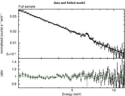
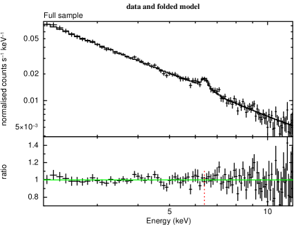
Figure 8: Full sample. Top panel: Fit with $E_{fixed}-\sigma_{fixed}$. Bottom panel: fit with the ’two-component model’.

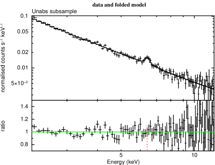
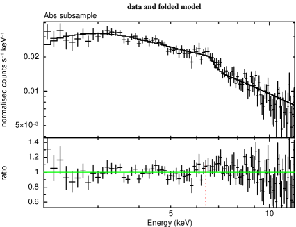
Figure 9: Fit with the ’two-component model’. Top panel: fit of the Unabs subsample. Bottom panel: fit to the Abs subsample.

Figure 10: Fit with the ’two-component model’. Top panel: subsample with z$<$1. Bottom panel: subsample with z$\geq$1.

Figure 11: Fit with the ’two-component model’. Top panel: Sey subsample. Bottom panel: QSO subsample.

The fits to our data and the ratios between data and model are shown in Figs. from 8 to 10; the corresponding fit results are given in Table 4. In the figures, a dotted vertical line has been placed at 6.4 keV energy for reference. In Fig. 8, we present, for comparison, the fits to the narrow Gaussian centred at 6.4 keV (the $E_{fixed}-\sigma_{fixed}$ described in the previous paragraph) in the top panel and the fits to the two-component model in the second panel. The fit is visually very similar in both cases. This impression is confirmed by looking at the first row of Table 4 that shows that, although the fit is better including both components, the improvement is statistically significant only at $2.1\sigma$.

The formal 90% confidence levels on the EW of both components almost reach zero in all cases, this is a consequence of the very strong coupling between their fluxes, as will be discussed below (see also Fig. 12).
We show in the last two columns of Table 4 the $\chi^{2}/\nu$ and the EW of the relativistic component obtained after setting the flux of the narrow component to zero.

4.2.3 Fits with comprehensive models

We finally made a test using a full-inclusive model that considers the entire set of spectral components expected in AGNs: the iron K_α at 6.4 keV, the Fe K_β at 7.05 keV, the Ni K_α at 7.47 keV, the Compton shoulder to the Fe K_α (approximated to be a Gaussian at 6.3 keV with width 35 eV) and the Compton reflection component of the continuum. This last component describes reflection in a slab geometry. The full-inclusive model, namely pexmon, was presented by Nandra et al. (2007). We used two pexmon components to consider reprocessing from material close to the central engine and far away from it. If the emission comes from the innermost regions, the pexmon will be smeared by the relativistic effects due to the proximity of the central SMBH. To account for these effects we convolved one pexmon component with the relativistic kernel kdblur2 which smears both the fluorescent lines and the Compton reflection. The resulting model will be absorbed by circumnuclear material (pha model). The second pexmon component, instead, will not be smeared or absorbed because it originates in external regions.

The convolution model kdblur2 used here has a similar set-up to that of Nandra et al. (2007) to allow a useful comparison with iron lines detected in individual spectra of AGN with high spectral quality. The model considers two emissivity laws, with slopes of 0 and 3, and a break radius which defines the border between the two regions initially fixed to 20 $R_{g}$ for simplicity. We considered an accretion disk around a maximally rotating BH, extended from 1.235 to 400 $R_{g}$, to allow a comparison with the results presented in the previous paragraph. We then thawed the inner radius and the break radius, but the results do not change significantly: in the first case we found an inner radius of $<62R_{g}$ with $\chi^{2}/dof=83.9/93$ ; in the second case we obtained a break radius of $<131R_{g}$ with $\chi^{2}/dof=84.1/93$.

The comprehensive model just described allows a description of the continuum more accurate than the phenomenological and the ’two component’ model. The values of the photon index increase from 1.63${}^{+0.03}_{-0.09}$ reported in Table 3 to the 1.71$\pm$0.06 value of Table 5, although they remain compatible within their error bars. The reflection factors and their 90% confidence limits, -0.35$\pm$0.18 and 0.45${}^{+0.38}_{-0.35}$, are both different from zero, suggesting that the two components have been found (see Sect. 5.4).

5 Discussion

We discuss in this Section the results obtained with the simulations, with the fits to a phenomenological model, and with the fits to physically-motivated models.

5.1 Discussion based on the simulations

Accurate modelling of the continuum is critical in determining the iron line properties of AGN and for this reason we developed a new method to do it independently of the spectral fitting. The EW discussed here are estimated with respect to a continuum integrated between 5.5 and 7. keV in the full sample (see Sect. 4.1). We expect at least two Fe line components within 5.5 and 7.0 keV: a narrow Fe line from neutral material with EW of 50-100 eV ubiquitously seen both in nearby and distant AGN (Nandra et al. 2007; Corral et al. 2008, 2011) and a broad line component with a distribution spanning from virtually zero to 300 eV and a median around 170 eV, as in the Seyferts sample of de la Calle Pérez et al. (2010). The EW of 203${}^{+33}_{-30}$ eV found in the full sample is therefore entirely consistent with having both components and, most importantly, not consistent with having only a narrow component (which is invariably smaller than 100 eV in AGN at low redshift). The estimates of the total EW in the subsamples also are compatible with the expected values, because the EW range from 71 eV (in the QSO subsample) to 283 eV (in the z$<$1 subsample).

In addition, the EW estimated with our simulations are generally higher when using a broader spectral window, which is compatible with the presence of a broad emission line.

5.2 Discussion based on phenomenological models

We considered a simple phenomenological Gaussian to fit the iron line and calculated the EW considering a monochromatic continuum at 6.4 keV. In these fits, we found that it is required by the data with high significance: from the spectral fitting to a simple Gaussian, the improvement of adding the Gaussian to the continuum is at $1-P(\Delta\nu,\Delta\chi^{2})=9\times 10^{-12}$ in the full sample (see Table 3), value that corresponds to a $6.8\sigma$ confidence level. The EW for the narrow line, is 95$\pm$22 eV for the full sample and lays between 77$\pm$35 eV (for the Abs subsample) and 167$\pm$67 eV (for the z$<1$ subsample): again, such values are consistent with those of fluorescent lines from material far away from the central BH.

Allowing for a broad neutral line ($E_{fixed}$-$\sigma_{free}$ second row of each subsample in Table 3), the errors on the line physical width could not be constrained in the full sample and in the majority of its subsamples: the upper limit of $\sim 300$ eV found in the full sample indicates that we cannot exclude the presence a broad line component in our detected lines although we are not able to constrain its properties. Looking at Table 3, Col. 4, the subsamples where a significance higher than $3\sigma$ is found in the fit with $E_{fixed}-\sigma_{free}$ (second row of each subsample) are the Abs subsample and QSO subsample. In both cases, there is a degeneracy between the iron line and the reflection component.

The EW values obtained from the fits with $E_{fix}$-$\sigma_{free}$ generally are in agreement with those found in previous works based on averaging methods, e.g. Corral et al. (2008), being of 107$\pm$50 eV in the full sample. A minimum of 36 % of this value is in principle the contribution from lines other than the K_α neutral iron line, such as the Fe K_β, the Ni K_α, the Compton Shoulder of the Fe K_α (Matt 2002), and that is expected to contribute to the detected line. The EW of 107$\pm$50 eV estimated for the full sample would mean that the contribution of the K_α iron line only is EW $\sim$69 eV. We expect EW encompassing a range of values from about 50 eV to 100 eV for non-obscured AGN, including the measurements presented here.

Investigating subsamples in luminosity and redshift, we found a hint of a difference in the line EW between the Seyferts subsample and the QSOs one: the line EW, for example in the second line of each sample in Table 3, is 88$\pm$32 eV in QSOs and 292$\pm$102 in Seyferts. Thus, the EW decreases with the increasing luminosity of the X-ray continuum in agreement with previous results for narrow (Iwasawa & Taniguchi 1993) and broad lines (Jiménez-Bailón et al. 2005). A similar result is found also from the model-independent estimates of the EW presented in the third column of Table 2.

In most cases, if the line width is left free to vary in the spectral fitting, its best fit value becomes higher than zero, as discussed above; on the contrary, if the centroid energy is left free, its output value does not differ from the input 6.4 keV energy (see second and third lines of Table 3). This indicates that the majority of the line flux is emitted for fluorescence from neutral iron.

The EW values (e.g. focusing on the $E_{fixed}-\sigma_{fixed}$ fitting presented in Col 9 of Table 3) are consistent with the ones calculated making use of the simulations, presented in Table 2, and explained in Sect. 4.1: this confirms that our estimates are robust.

The EW measured in this work are broadly consistent with the values of individual bright sources in the literature: this confirms that the iron lines are emitted by the majority of the sources in our sample because the EW of the minority Iron-line-emitting sources would be much higher than that observed in individual sources. Our resulting EW are also consistent with previous estimates made in iron line stacking, e.g. in Corral et al. (2008).

5.3 Discussion based on physical models

We used a model more specific than a simple Gaussian to fit our data and calculated the EW considering a monochromatic continuum. The ’physical’ model is composed by a narrow core centred at 6.4 keV and a relativistic component (diskline in xspec).

This two-component model is expected in AGN, where reflection of the primary emission is expected to occur both in axis-symmetric regions far away from the BH (such as the torus) and close enough to it for the detection of any line broadening, e.g. in the accretion disk (Fabian et al. 1989). Both components are in principle expected. Our values of the EW reported in Table 4 support this, being consistent with previous results based on averaging techniques and on the study of individual higher quality spectra of AGN in the local Universe. Moreover, our model-independent estimates between 173 and 236 eV (full sample, bulk range in Table 2) are inconsistent with having only a narrow component, which does not commonly exceed 100 eV in the local Universe. This provides an interesting indication, independent of the spectral fitting, of the presence of a relativistic line component in the XMM CDFS data. However, the improvement of the fit by including the relativistic component (Col. 3 in Table 4) is not statistically significant (e.g., for the full sample, 2.1 $\sigma$ confidence level), so we have not formally detected a broad component our samples. Having said that, the two line components are strongly correlated and we cannot really disentangle them: we can see the 1, 2, 3 $\sigma$ contours (for two interesting parameters) for the full sample in the space formed by the EW of the relativistic line and that of the narrow line in Fig. 12 (top panel). There are equally-good fits including only each of the components or a combination of both for most samples (see cols. 1, 2 and 9 of Table 4).

It is important to notice that our contours (shown for the full sample) exclude the point with zero EW simultaneously for both components at much more than three $\sigma$ confidence level. This indicates a very secure detection of an iron line feature.

For the full sample, the EW of the narrow line with no relativistic component is $95\pm 22$ eV (see first row of Table 3) while the EW of the relativistic line fixing the flux of the narrow line to zero is $347\pm 105$ eV (Col. 10 in Table 4, first row). These results are, within the uncertainties, compatible with the measurements and upper limits found in Corral et al. (2008) and Chaudhary et al. (2012). Taking into account that our values include contributions of fluorescence in material close to the central SMBH and in outer regions that we are not able to disentangle, they are also consistent, considering the error bars, with the ”average” EW=76-143 eV of the relativistic lines detected in individual sources in de la Calle Pérez et al. (2010).

5.4 Discussion based on comprehensive models

We fitted the average spectra with a more complete model with two reflection components. The first one is emitted from the innermost regions of AGN and smeared by relativistic effects due to the vicinity of the central SMBH, the second component is instead emitted from outer regions and is un-blurred. The reflection factor contours at 1, 2, 3 sigma, are shown in Fig. 12, bottom panel. The figure shows that the relativistic component is different from zero at two sigma confidence level, and the non-relativistic one at three sigma.The two components are coupled: like the above described ’two component’ model of the iron line, these cannot be accurately disentangled. Anyway, we should note that the point with zero reflection factor for both components is excluded at much more than three sigma confidence level, indicating a secure, highly significant detection of reflection features.

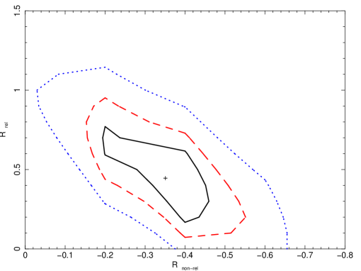
Figure 12: Contours at 1 (continuous line), 2 (dashed line), 3 (dotted line) sigma of the EW of the narrow and the relativistic line in the ’two-component model’ (top panel). Same contours for the reflection factor $R$ of both the non-relativistic and the relativistic components of the comprehensive model (bottom panel).

6 Conclusions

We studied a representative sample of 54 AGN (100 spectra from XMM-Newton) with the best spectral S/N in the ultra-deep observation of the Chandra Deep Field South. We investigated several subsamples: two subsamples of column density of the intrinsic absorber (borderline at $\log{\left(N_{\rm H}\right)}=21.5$), two subsamples in luminosity (with cut at $\log{\left(L\right)}=44$), and finally two in redshift (segregated at $z=1$).

We averaged the spectra of the full sample and subsamples developing further our own method previously used in Corral et al. (2008) and Falocco et al. (2012) to characterise the instrumental and averaging effects. To do this we made use of comprehensive simulations.

With our new methodology and best data quality so far we could find convincing and solid evidence, using X-ray stacking, for a highly significant iron line in distant AGN, taking into full account the instrumental and methodological effects. In the spectral fits we convolved our models with a gaussian smoothing with a variable $\Sigma(E)$ introduced by the limited spectral resolution of the X-ray instruments and the averaging process.

We can summarise our conclusions as follows:

• The iron feature is significantly detected in the full sample and in all its subsamples.

• The iron line, modelled with an unresolved Gaussian at 6.4 keV (as expected from neutral material far from the central BH), is detected at 6.8$\sigma$ in the full sample, with EW=$95\pm 22$ eV. In the subsamples, the EW measurement ranges from 77 eV for Abs (our objects with $\log{\left(N_{H}\right)}\geq 21.5$) and 167 eV for the sources with $z<1$ respectively. We find evidence for the Iwasawa-Taniguchi effect comparing the EW of the low luminosity (Seyfert) and high luminosity (QSO) samples. Allowing for a resolved Gaussian profile improves the fit slightly, but not significantly ($\la 2\sigma$).

• Using a combination of an unresolved line from neutral iron as above and a relativistic line, to take reflection in material far and close to the central BH into account, we found again that the broad component, despite improving the fit moderately in most cases, is not formally required. However, we also found that the fitted parameters of both components are strongly coupled, finding good fits with either or both components. We cannot really disentangle both contributions with our current data. Using a single relativistic component with no unresolved line, we find EW$=347\pm 105$ eV for the full sample.

• The EW of the narrow iron line and that of our tentative relativistic line are both broadly consistent with those (including the upper limits) estimated in previous works based on averaging and stacking methods (Corral et al. 2008; Chaudhary et al. 2012) and in individual bright sources in the literature (de la Calle Pérez et al. 2010), which leads to the conclusion that an iron feature must be widespread among spectra of AGN.

• The model-independent EW estimates made using our thorough simulations produce similar values as those from model fitting described above, confirming the robustness of the results presented in this paper. Interestingly, the EW is inconsistent with having a narrow line only and becomes higher when a broader energy range around the line centroid is considered. This suggests the presence of a broad iron feature.

Concluding, although the observed lines are well modelled as fluorescent lines at 6.4 keV in material far away from the primary emission, we found also some tentative evidence for a component emitted relatively close to the SMBH. Our work has confirmed that high S/N and a large amount of spectral counts are required to characterise average iron features in distant AGN. For a more detailed characterisation of its physical origin, it is necessary to accumulate a higher number of spectral counts in the average spectrum.

Although the complexity of the X-ray AGN spectra often makes challenging the determination of the properties of iron features, with the deepest XMM-Newton data available and a careful characterisation of methodological effects, we have confirmed that iron emission lines represent a universal feature of AGN in the distant Universe.

Table 3: Results of fits of the average spectrum of the full sample and its subsamples with gsmooth$\otimes$(pha$\times$pex+gauss).

Sample	$\chi^{2}$/$\nu$(c)	$\chi^{2}$/$\nu$(g)	$1-P(\Delta\nu,\Delta\chi^{2})$	$\mathrm{N_{\rm H}}$	$\Gamma$	$R$	E	$\sigma$	EW	$\langle z\rangle$	$\langle\log{\left(L\right)}\rangle$
				$10^{22}$cm-2	-		keV	eV	eV		erg s-1
(1)	(2)	(3)	(4)	(5)	(6)	(7)	(8)	(9)	(10)	(11)	(12)
Full	133.4/95	87.0/94	$9\times 10^{-12}$ ($6.8\sigma$)	$0.36^{+0.17}_{-0.27}$	$1.63^{+0.03}_{-0.09}$	$1.00^{+4.50}_{-0.65}$	$\equiv$6.4	$\equiv$0	95$\pm 22$	1.34	43.74
		86.2/93	[$0.4$ ($0.9\sigma$)]	$0.36\pm 0.22$	$1.63^{+0.04}_{-0.08}$	$1.0^{+3.8}_{-1.0}$	$\equiv$6.4	$92^{+236}_{-92}$	107$\pm 50$
		87.0/93	[$1$ ($0\sigma$)]	$0.36\pm 0.21$	$1.63\pm 0.06$	$1.0^{+4.1}_{-0.6}$	6.4$\pm$0.20	$\equiv 0$	94$\pm 22$
		85.9/92	[$0.6$ ($0.52\sigma$)]	$0.36\pm 0.21$	$1.63\pm 0.05$	$1.0^{+3.7}_{-1.0}$	6.44${}_{-0.10}^{+0.04}$	$91_{-87}^{+197}$	$109\pm 44$
Unabs	139.2/95	108.7/94	$3\times 10^{-8}$ ($5.5\sigma$)	$<0.82$	$1.87\pm 0.03$	$1.0\pm 0.4$	$\equiv$6.4	$\equiv$0	$107\pm 32$	1.27	43.78
		108.7/93	[$1$ ($0\sigma$)]	$<0.82$	$1.87\pm 0.03$	$1.0^{+0.2}_{-0.2}$	$\equiv$6.4	$1^{+822}_{-1}$	$107\pm 32$
		108.7/93	[$1$ ($0\sigma$)]	$<0.82$	$1.87\pm 0.03$	$1.0^{+0.2}_{-0.2}$	$6.4_{-0.1}^{-0.4}$	$\equiv$0	$107\pm 32$
		108.7/92	[$1$ ($0\sigma$)]	$<0.82$	$1.88\pm$0.03	$1^{+0.2}_{-0.2}$	$6.4_{-0.1}^{+0.3}$	$5_{-5}^{+800}$	$107\pm 32$
Abs	109.4/95	94.2/94	$1\times 10^{-4}$ ($3.9\sigma$)	$3.67\pm$0.55	$1.49\pm 0.08$	$1^{+3.6}_{-1}$	$\equiv$6.4	$\equiv$0	$77\pm 34$	1.28	43.74
		85.4/93	[$3\times 10^{-3}$ ($3\sigma$)]	$3.39\pm$0.53	$1.39\pm$0.08	$0.003^{+1.100}_{-0.001}$	$\equiv$6.4	$455^{+294}_{-187}$	$243\pm 123$
		94.2/93	[$1$ ($0\sigma$)]	$3.67\pm 0.55$	$1.52^{+0.10}_{-0.09}$	$1^{+3.7}_{-1}$	$6.4\pm 0.2$	$\equiv$0	$77\pm 32$
		85.6/92	[$3\times 10^{-3}$ ($2.9\sigma$)]	$3.42\pm 0.54$	$1.39\pm 0.08$	$0.003^{+1.050}_{-0.003}$	$6.47\pm 0.20$	$438^{+273}_{-192}$	$239\pm 109$
z$<$1	112.6/95	97.0/94	$8\times 10^{-5}$ ($3.9\sigma$)	$0.86\pm 0.40$	$1.58\pm 0.08$	$1.0^{+13.5}_{-1.0}$	$\equiv$6.4	$\equiv$0	167$\pm$67	0.64	43.21
		94.0/93	[$0.08$ ($1.7\sigma$)]	$0.92\pm 0.40$	$1.56\pm 0.08$	$1.0^{+7.5}_{-0.6}$	$\equiv$6.4	$4^{+150}_{-4}$	81$\pm 34$
		94.0/93	[$0.08$ ($1.7\sigma$)]	$0.92\pm 0.40$	$1.56\pm 0.08$	$1.0^{+7.5}_{-0.6}$	6.4${}^{+0.6}_{-0.4}$	$\equiv$0	81$\pm 34$
		94.0/92	[$0.22$ ($1.2\sigma$)]	$0.92\pm 0.40$	$1.56\pm 0.08$	$1.0^{+0.9}_{-0.6}$	6.40$\pm_{-0.13}^{+0.28}$	$2_{-2}^{+822}$	$81\pm 34$
z$\geq$1	109.9/95	78.5/94	$2\times 10^{-8}$ ($5.6\sigma$)	$<0.24$	$1.63\pm 0.06$	$0.3^{+1.6}_{-0.3}$	$\equiv$6.4	$\equiv$0	114$\pm 30$	1.80	44.07
		76.2/94	[$0.1$ ($1.5\sigma$)]	$<0.32$	$1.60\pm 0.05$	$0.008^{+1.300}_{-0.008}$	$\equiv$6.4	$150^{+100}_{-152}$	114$\pm 42$
		78.5/93	[$1$ (0$\sigma$)]	$<0.441$	$1.63^{+0.11}_{-0.04}$	$0.3^{+1.7}_{-0.3}$	6.40${}^{+0.25}_{-0.25}$	$\equiv$0	150$\pm 40$
		76.2/92	[$0.32$ ($1\sigma$)]	$<0.32$	$1.60^{+0.05}_{-0.04}$	$0.008_{-0.008}^{+1.400}$	6.40${}^{+0.10}_{-0.07}$	$151^{+117}_{-151}$	$150\pm 55$
Sey	129.9/95	93.9/94	$2\times 10^{-9}$ ($6\sigma$)	$0.36^{-0.30}_{-0.29}$	$1.58\pm 0.07$	$1.0^{+2.5}_{-0.8}$	$\equiv$6.4	$\equiv$0	103$\pm 27$	0.91	43.35
		90.6/93	[$0.066$ ($1.84\sigma$)]	$<0.47$	$1.51\pm 0.07$	$0.004_{-0.004}^{+1.800}$	$\equiv$6.4	$450^{+200}_{-200}$	293$\pm 102$
		93.9/93	[$1$ ($0\sigma$)]	$0.36^{+0.29}_{-0.29}$	$1.58\pm 0.07$	$1.0_{-0.8}^{+2.5}$	6.40${}_{-0.05}^{+0.05}$	$\equiv$0	103$\pm 27$
		90.4/92	[$0.17$ ($1.4\sigma$)]	$<0.56$	$1.51\pm 0.06$	$0.004_{-0.004}^{+1.800}$	$6.5_{-0.20}^{+0.09}$	425$\pm 187$	289$\pm 96$
QSO	204.2/95	178.2/94	$3\times 10^{-7}$ ($5.10\sigma$)	$0.11^{+0.23}_{-0.08}$	$1.60_{-0.02}^{+0.07}$	$0.14_{-0.14}^{+1.36}$	$\equiv$6.4	$\equiv$0	119$\pm 30$	2.02	44.34
		166.6/93	[$5.3\times 10^{-4}$ ($3.5\sigma$)]	$0.20\pm 0.15$	$1.65\pm 0.04$	$0.66^{+1.34}_{-0.04}$	$\equiv$6.4	$101^{+120}_{-100}$	88$\pm 32$
		167.3/93	[$9\times 10^{-4}$ ($3.3\sigma$)]	$0.24\pm 0.15$	$1.68\pm 0.4$	$0.9^{+1.3}_{-0.8}$	6.40${}_{-0.15}^{+0.05}$	$\equiv$0	75$\pm 22$
		164.9/92	[$0.0013$ ($3.22\sigma$)]	$0.19\pm 0.15$	$1.65\pm 0.04$	$0.61^{+0.30}_{-0.30}$	6.34${}_{-0.07}^{+0.07}$	$130^{+89}_{-112}$	$93\pm 31$

Table 4: Fits results of the average spectrum of the full sample and subsamples using gsmooth$\otimes[$pha$\times$(pex+laor)+gaus)$]$.

Sample	$\chi^{2}_{g}$/$\nu$	$\chi^{2}$/$\nu$	$1-P(\Delta\nu,\Delta\chi^{2})$	$\mathrm{N_{\rm H}}$	$\Gamma$	$Rel_{refl}$	EWrel	EWna	$\chi^{2}_{one-rel}$/$\nu$	EWone-rel
				1022cm-2			eV	eV		eV
(0)	(1)	(2)	(3)	(4)	(5)	(6)	(7)	(8)	(9)	(10)
Full	87.0/94	82.6/93	3.6$\times 10^{-2}$($2.1\sigma$)	$0.24\pm 0.24$	$1.61\pm 0.06$	$1.0_{-1.0}^{+2.3}$	$140\pm 120$	$67\pm 28$	98.4/94	$347\pm 105$
Unabs	108.7/94	108.7/93	1($0\sigma$)	$<0.82$	$1.87\pm 0.03$	$1_{-0.2}^{+0.4}$	$0_{-0}^{+1000}$	$107_{-32}^{+32}$	138.9/94	$0_{-0}^{+1000}$
Abs	94.2/94	92.6/93	0.2($1.3\sigma$)	$2.84\pm 0.60$	$1.29\pm 0.08$	$0._{-0}^{+2}$	$404\pm 140$	$<1000$	92.6/94	$404\pm 140$
z$<$1	97.0/94	95.2/93	0.2($1.3\sigma$)	$0.68\pm 0.40$	$1.55\pm 0.09$	$1_{-1}^{+4}$	$173\pm 173$	$104\pm 93$	99.7/94	$362\pm 210$
z$\geq$1	78.5/94	77.6/93	0.3($1\sigma$)	$<0.3$	$1.58\pm 0.04$	$0.007_{-0.007}^{+1.680}$	$84\pm 84$	$98_{-31}^{+31}$	94.6/94	$318\pm 119$
Sey	93.9/94	92.2/93	0.2($1.3\sigma$)	$0.26^{+0.32}_{-0.26}$	$1.57\pm 0.07$	$1_{-1}^{+6}$	$118\pm 118$	$82_{-35}^{+35}$	107.6/94	$380\pm 130$
QSO	178.2/94	166.7/93	7$\times 10^{-4}$($3.4\sigma$)	$<0.138$	$1.58\pm 0.08$	$0.13_{-0.13}^{+0.80}$	$228\pm 70$	$49\pm 45$	169.7/94	$316\pm 82$

Table 5: Fits results of the average spectrum of the full sample and subsamples using gsmooth$\otimes[$ pha $\times$ kdblur2 $\otimes$(pexm)+pexm)$]$ .

Sample	$\chi^{2}$/$\nu$	$\mathrm{N_{\rm H}}$	$\Gamma$	$R_{non-rel}$	$R_{rel}$
(0)	(1)	(2)	(3)	(4)	(5)
Full	84.1/94	0.46$\pm 0.03$	1.71$\pm$0.06	-0.35$\pm$0.18	0.45${}_{-0.35}^{+0.38}$
Unabs	104.0/94	$<$0.10	1.95$\pm$0.06	-0.50$\pm$0.27	0.43${}_{-0.43}^{+0.54}$
Abs	90.2/94	3.68 $\pm$0.53	1.56$\pm$0.09	-0.167${}_{-0.228}^{+0.168}$	$0.59_{-0.46}^{+0.51}$
z$<1$	91.5/94	1.01$\pm$0.40	1.65$\pm$0.10	-0.317$\pm$0.220	$0.46_{-0.43}^{+0.49}$
z$\geq 1$	80.5/94	0.343$\pm$0.290	1.76$\pm$0.07	-0.53$\pm$0.23	$0.08_{-0.08}^{+0.48}$
Sey	89.0/94	0.48$\pm$0.30	1.69$\pm$0.09	-0.39$\pm$0.22	$0.54\pm 0.45$
QSO	73.9/94	0.57$\pm$0.32	1.76$\pm$0.08	-0.33$\pm$0.26	0.16${}_{-0.16}^{+0.49}$

References

- Arnaud (1996) Arnaud, K. A. 1996, in Astronomical Society of the Pacific Conference Series, Vol. 101, Astronomical Data Analysis Software and Systems V, ed. G. H. Jacoby & J. Barnes, 17
- Balestra et al. (2010) Balestra, I., Mainieri, V., Popesso, P., et al. 2010, A&A, 512, A12
- Ballantyne (2010) Ballantyne, D. R. 2010, ApJ, 708, L1
- Bardeen et al. (1972) Bardeen, J. M., Press, W. H., & Teukolsky, S. A. 1972, ApJ, 178, 347
- Brusa et al. (2005) Brusa, M., Gilli, R., & Comastri, A. 2005, ApJ, 621, L5
- Caccianiga et al. (2007) Caccianiga, A., Severgnini, P., Della Ceca, R., et al. 2007, A&A, 470, 557
- Carrera et al. (2007) Carrera, F. J., Ebrero, J., Mateos, S., et al. 2007, A&A, 469, 27
- Carter & Read (2007) Carter, J. A. & Read, A. M. 2007, A&A, 464, 1155
- Casey et al. (2011) Casey, C. M., Chapman, S. C., Smail, I., et al. 2011, MNRAS, 411, 2739
- Chaudhary et al. (2010) Chaudhary, P., Brusa, M., Hasinger, G., Merloni, A., & Comastri, A. 2010, A&A, 518, A58
- Chaudhary et al. (2012) Chaudhary, P., Brusa, M., Hasinger, G., et al. 2012, A&A, 537, A6
- Civano et al. (2005) Civano, F., Comastri, A., & Brusa, M. 2005, MNRAS, 358, 693
- Comastri et al. (2011) Comastri, A., Ranalli, P., Iwasawa, K., et al. 2011, A&A, 526, L9
- Cooper et al. (2011) Cooper, M. C., Aird, J. A., Coil, A. L., et al. 2011, ApJS, 193, 14
- Corral et al. (2011) Corral, A., Della Ceca, R., Caccianiga, A., et al. 2011, A&A, 530, A42
- Corral et al. (2008) Corral, A., Page, M. J., Carrera, F. J., et al. 2008, A&A, 492, 71
- de la Calle Pérez et al. (2010) de la Calle Pérez, I., Longinotti, A. L., Guainazzi, M., et al. 2010, A&A, 524, A50
- Della Ceca et al. (2004) Della Ceca, R., Maccacaro, T., Caccianiga, A., et al. 2004, A&A, 428, 383
- Ebrero et al. (2009) Ebrero, J., Carrera, F. J., Page, M. J., et al. 2009, A&A, 493, 55
- Fabian et al. (1989) Fabian, A. C., Rees, M. J., Stella, L., & White, N. E. 1989, MNRAS, 238, 729
- Falocco et al. (2012) Falocco, S., Carrera, F. J., Corral, A., et al. 2012, A&A, 538, A83
- Guainazzi et al. (2011) Guainazzi, M., Bianchi, S., de La Calle Pérez, I., Dovčiak, M., & Longinotti, A. L. 2011, A&A, 531, A131
- Guainazzi et al. (2006) Guainazzi, M., Bianchi, S., & Dovčiak, M. 2006, Astronomische Nachrichten, 327, 1032
- Haberl et al. (2002) Haberl, F., Briel, U. G., Dennerl, K., & Zavlin, V. E. 2002, ArXiv Astrophysics e-prints (arXiv:astro-ph/0203235)
- Iwasawa et al. (2012) Iwasawa, K., Mainieri, V., Brusa, M., et al. 2012, A&A, 537, A86
- Iwasawa & Taniguchi (1993) Iwasawa, K. & Taniguchi, Y. 1993, ApJ, 413, L15
- Jiménez-Bailón et al. (2005) Jiménez-Bailón, E., Piconcelli, E., Guainazzi, M., et al. 2005, A&A, 435, 449
- Kriek et al. (2008) Kriek, M., van Dokkum, P. G., Franx, M., et al. 2008, ApJ, 677, 219
- Laor (1991) Laor, A. 1991, ApJ, 376, 90
- Le Fèvre et al. (2005) Le Fèvre, O., Guzzo, L., Meneux, B., et al. 2005, A&A, 439, 877
- Le Fèvre et al. (2004) Le Fèvre, O., Vettolani, G., Paltani, S., et al. 2004, A&A, 428, 1043
- Mateos et al. (2008) Mateos, S., Warwick, R. S., Carrera, F. J., et al. 2008, A&A, 492, 51
- Matt (2002) Matt, G. 2002, MNRAS, 337, 147
- Mignoli et al. (2005) Mignoli, M., Cimatti, A., Zamorani, G., et al. 2005, A&A, 437, 883
- Nandra et al. (1997) Nandra, K., George, I. M., Mushotzky, R. F., Turner, T. J., & Yaqoob, T. 1997, ApJ, 488, L91
- Nandra et al. (2007) Nandra, K., O’Neill, P. M., George, I. M., & Reeves, J. N. 2007, MNRAS, 382, 194
- Nandra et al. (2006) Nandra, K., O’Neill, P. M., George, I. M., Reeves, J. N., & Turner, T. J. 2006, Astronomische Nachrichten, 327, 1039
- Press et al. (1992) Press, W. H., Teukolsky, S. A., Vetterling, W. T., & Flannery, B. P. 1992, Numerical recipes in FORTRAN. The art of scientific computing (Cambridge: University Press, —c1992, 2nd ed.)
- Ranalli et al. (2013) Ranalli, P., Comastri, A., Vignali, C., et al. 2013, ArXiv e-prints (1304.5717)
- Ravikumar et al. (2007) Ravikumar, C. D., Puech, M., Flores, H., et al. 2007, A&A, 465, 1099
- Silverman et al. (2010) Silverman, J. D., Mainieri, V., Salvato, M., et al. 2010, ApJS, 191, 124
- Stark et al. (1992) Stark, A. A., Gammie, C. F., Wilson, R. W., et al. 1992, ApJS, 79, 77
- Streblyanska et al. (2005) Streblyanska, A., Hasinger, G., Finoguenov, A., et al. 2005, A&A, 432, 395
- Szokoly et al. (2004) Szokoly, G. P., Bergeron, J., Hasinger, G., et al. 2004, ApJS, 155, 271
- Tanaka et al. (1995) Tanaka, Y., Nandra, K., Fabian, A. C., et al. 1995, Nature, 375, 659
- Taylor et al. (2009) Taylor, E. N., Franx, M., van Dokkum, P. G., et al. 2009, ApJS, 183, 295
- Treister et al. (2009) Treister, E., Virani, S., Gawiser, E., et al. 2009, ApJ, 693, 1713
- Ueda et al. (2003) Ueda, Y., Akiyama, M., Ohta, K., & Miyaji, T. 2003, ApJ, 598, 886
- van der Wel et al. (2005) van der Wel, A., Franx, M., van Dokkum, P. G., et al. 2005, ApJ, 631, 145
- Vanzella et al. (2008) Vanzella, E., Cristiani, S., Dickinson, M., et al. 2008, A&A, 478, 83
- Watson et al. (2008) Watson, M. G., Schroder, A. C., Fyfe, D., et al. 2008, VizieR Online Data Catalog, 349, 30339