The prospects of forming ultracold molecules in ${}^{2}\Sigma$ states
by magnetoassociation of alkali-metal atoms with Yb

Abstract

We explore the feasibility of producing ultracold diatomic molecules with nonzero electric and magnetic dipole moments by magnetically associating two atoms, one with zero electron spin and one with nonzero spin. Feshbach resonances arise through the dependence of the hyperfine coupling on internuclear distance. We survey the Feshbach resonances in diatomic systems combining the nine stable alkali-metal isotopes with those of Yb, focussing on the illustrative examples of RbYb and CsYb. We show that the resonance widths may expressed as a product of physically comprehensible terms in the framework of Fermi’s Golden Rule. The resonance widths depend strongly on the background scattering length, which may be adjusted by selecting the Yb isotope, and on the hyperfine coupling constant and the magnetic field. In favorable cases the resonances may be over 100 mG wide.

I Introduction

The successes of cooling gases of atoms to ultracold temperatures have led to great interest in producing molecules at similar temperatures. Because molecules have a richer internal structure and more complex interactions than atoms, ultracold ($\mu$K) molecules offer the possibility of exploring a wide range of new research areas, including high-precision measurement Hudson et al. (2006); Kawall et al. (2004); Hudson et al. (2002), quantum information DeMille (2002); Jaksch et al. (1999) and quantum simulation Micheli et al. (2006).

Molecules may be formed in ultracold atomic gases either by photoassociation Jones et al. (2006) or by magnetoassociation Köhler et al. (2006). In the latter, cold atomic clouds are subjected to time-dependent magnetic fields that convert atom pairs into molecules by adiabatic passage across zero-energy Feshbach resonances Chin et al. (2010). Recent years have seen substantial progress in producing ultracold molecules made up of pairs of alkali-metal atoms Herbig et al. (2003); Regal et al. (2003); Strecker et al. (2003); Cubizolles et al. (2003); Jochim et al. (2003); Ni et al. (2008); Danzl et al. (2010); Lang et al. (2008); Heo et al. (2012). The molecules are left in high vibrational states and are susceptible to collisional trap loss. For KRb Ni et al. (2008), Cs₂ Danzl et al. (2010), and triplet Rb₂ Lang et al. (2008), it has been possible to transfer the molecules to the absolute ground state by Stimulated Raman Adiabatic Passage (STIRAP).

There is now great interest in the formation of cold molecules that have both electric and magnetic dipole moments Żuchowski et al. (2010); Ivanov et al. (2011); Hansen et al. (2011); Hara et al. (2011); Nemitz et al. (2009); Brue and Hutson (2012). Such molecules offer additional possibilities for manipulation, trapping, and control because they can be influenced by both electric and magnetic fields. In the present paper we investigate the prospects for magnetoassociation of alkali-metal atoms (Alk) with ¹S atoms (specifically Yb) to form ${}^{2}\Sigma$ heteronuclear diatoms with electron spin $S=1/2$.

Ytterbium is an excellent candidate for pairing with the alkali metals. It has 7 stable isotopes (5 zero-spin bosons, 2 fermions), and a closed-shell, singlet-spin electronic structure. Both bosonic Takasu et al. (2003); Fukuhara et al. (2007a, 2009); Sugawa et al. (2011) and fermionic Fukuhara et al. (2007b, c) isotopes have been cooled to quantum degeneracy. Different isotopic combinations have different scattering lengths, and produce molecules with different binding energies; they thus have Feshbach resonances at different magnetic fields.

The existence of magnetically tunable Feshbach resonances requires coupling between a continuum scattering state of the atomic pair and a molecular state that crosses it as a function of magnetic field. For pairs of alkali-metal atoms, this coupling is provided by the difference between the singlet and triplet potential curves and by the magnetic dipolar interaction between the electron spins. However, neither of these effects exists in systems of the type considered here. Instead, the most significant coupling between the atomic and molecular states is provided by the $R$-dependence in the hyperfine coupling constant of the alkali-metal atom Żuchowski et al. (2010). Such $R$-dependences exist in alkali dimers Strauss et al. (2010), but in that case they merely produce small shifts in bound state energies and resonance positions, rather than driving new resonances. If the closed-shell atom has non-zero nuclear spin, it can also couple to the unpaired electron spin. For the case of LiYb Brue and Hutson (2012), this coupling has been found to be much stronger than that due to the Li nucleus. However, this latter effect is less important for the heavier alkali-metal atoms considered here, where the coupling to the alkali-metal nucleus itself is stronger.

In previous work, we extracted resonance positions and widths for RbSr Żuchowski et al. (2010) and LiYb Brue and Hutson (2012) from coupled-channel quantum scattering calculations. In the present paper, we extend these studies to a range of heavier systems and show how the widths may be broken down into their contributing factors within the framework of Fermi’s Golden Rule.

The theoretical development presented here is applicable to any system made up of an alkali-metal atom paired with a closed-shell atom. In the present study, we have considered the whole range of Alk-Yb systems, but we focus our presentation on the illustrative examples of Rb-Yb, for which the scattering lengths are approximately known, and Cs-Yb, for which they are as yet unknown. In section II we describe the theoretical methods used. In section III we present our results, with discussion of system characteristics that lead to Feshbach resonances suitable for molecule formation.

II Theory

II.1 Collisions between alkali-metal and closed-shell atoms

The Hamiltonian for an alkali-metal atom $a$ in a ²S state, interacting with a closed-shell atom $b$ in a ¹S state, is

$$\hat{H}=\frac{\hbar^{2}}{2\mu}\left[-\frac{{\rm d^{2}}}{{\rm d}R^{2}}+\frac{\hat{L}^{2}}{R^{2}}\right]+\hat{U}(R)+\hat{H}_{a}+\hat{H}_{b}$$ (1)

where $\hat{L}$ is the two-atom rotational angular momentum operator and $\hat{U}(R)$ is the interaction operator. $\hat{H}_{a}$ and $\hat{H}_{b}$ are the single-atom hamiltonians,

$$H_{a} = \zeta_{a}\hat{i}_{a}\cdot\hat{s}+\left(g_{a}\mu_{\rm N}\hat{i}_{a,z}+g_{e}\mu_{\rm B}\hat{s}_{z}\right)B$$ (2)

$$H_{b} = g_{b}\mu_{\rm N}\hat{i}_{b,z}B,$$ (3)

where $\hat{s}$, $\hat{i}_{a}$ and $\hat{i}_{b}$ are the electron and nuclear spin operators, $g_{e}$, $g_{a}$ and $g_{b}$ are the electronic and nuclear $g$ factors, and $\mu_{\rm B}$ and $\mu_{\rm N}$ are the Bohr and nuclear magnetons. $\zeta_{a}$ is the hyperfine coupling constant for the alkali-metal atom and $B$ is the external magnetic field, whose direction defines the $z$ axis. In the present work we use lower-case angular momentum operators and quantum numbers for individual atoms and upper-case for the corresponding molecular quantities.

The interaction of a ²S atom with a ¹S atom produces only one molecular electronic state, of ${}^{2}\Sigma$ symmetry. However, the hyperfine coupling constant of the alkali-metal atom is modified by the presence of the closed-shell atom Żuchowski et al. (2010), and if $i_{b}\neq 0$ then there is also hyperfine coupling involving the nucleus of atom $b$ Brue and Hutson (2012),

$$\zeta_{a}(R) = \zeta_{a}+\Delta\zeta_{a}(R);$$ (4)

$$\zeta_{b}(R) = \Delta\zeta_{b}(R).$$ (5)

The interaction operator $\hat{U}(R)$ is thus

$$\hat{U}(R)=V(R)+\Delta\zeta_{a}(R)\hat{i}_{a}\cdot\hat{s}+\Delta\zeta_{b}(R)\hat{i}_{b}\cdot\hat{s},$$ (6)

where $V(R)$ is the electronic interaction potential. Most of the theory presented here remains applicable when atom $a$ is a non-alkali-metal atom in a multiplet-S state.

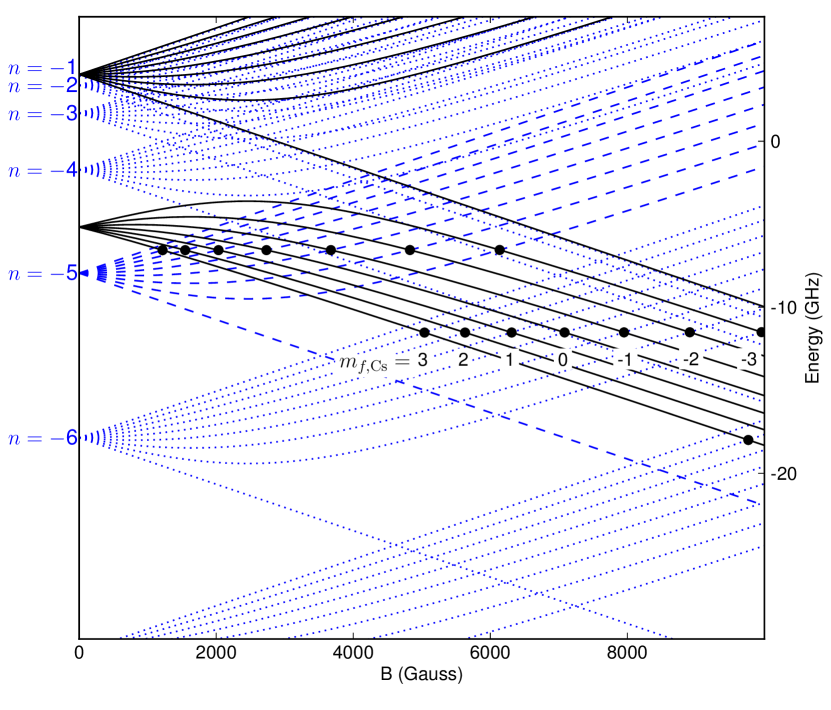
Figure 1: (color online). Hyperfine energy levels for ¹³³Cs in its ground ²S state (solid black lines) and for near-threshold states of CsYb arising from the upper hyperfine manifold $|\alpha_{2},m_{f,{\rm Cs}}\rangle$ (dashed blue lines), calculated for a potential with a scattering length of $-38$ bohr. The $n=-1$ level is almost hidden by the threshold. The solid circles mark the Feshbach resonances that occur at crossings between bound states and atomic thresholds with the same value of $m_{f,{\rm Cs}}$.

Figure 1 shows the energy levels of the ¹³³Cs atom, with $i_{a}=7/2$ (black solid lines). At zero field the levels may be labeled by quantum numbers $f_{a},m_{f,a}$, where $f_{a}=i_{a}\pm 1/2$, whereas at high field the nearly good quantum numbers are $m_{s,a}$ and $m_{i,a}$. In the present paper we indicate the lower and upper states for each $m_{f,a}=m_{s,a}+m_{i,a}$ as $|\alpha_{1},m_{f,a}\rangle$ and $|\alpha_{2},m_{f,a}\rangle$ respectively.

The Hamiltonian (1) may be written as the sum of a zeroth-order term $\hat{H}^{0}$ and a perturbation $\hat{H}^{\prime}$,

$$\hat{H}^{0} = \frac{\hbar^{2}}{2\mu}\left[-\frac{{\rm d}^{2}}{{\rm d}R^{2}}+\frac{\hat{L}^{2}}{R^{2}}\right]+V(R)+\hat{H}_{a}+\hat{H}_{b};$$ (7)

$$\hat{H}^{\prime} = \Delta\zeta_{a}(R)\hat{i}_{a}\cdot\hat{s}+\Delta\zeta_{b}(R)\hat{i}_{b}\cdot\hat{s}.$$ (8)

The zeroth-order Hamiltonian is separable, and its eigenfunctions are products of atomic functions $|\alpha_{i},m_{f,a}\rangle|i_{b},m_{i,b}\rangle$ and radial functions $\psi(R)$. The latter are eigenfunctions of the 1-dimensional Hamiltonian

$$\frac{\hbar^{2}}{2\mu}\left[-\frac{{\rm d}^{2}}{{\rm d}R^{2}}+\frac{L(L+1)}{R^{2}}\right]+V(R),$$ (9)

with eigenvalues $E_{n}$. The eigenvalues of $\hat{H}^{0}$ are $E_{n}+E_{a}+E_{b}$, where $E_{a}$ and $E_{b}$ are the eigenvalues of $\hat{H}_{a}$ and $\hat{H}_{b}$. By contrast with the alkali-metal dimers, the molecular states thus lie almost parallel to the atomic states as a function of magnetic field. They also have almost exactly the same spin character. The only terms in the Hamiltonian (1) that couple $|\alpha_{1},m_{f,a}\rangle|i_{b},m_{i,b}\rangle$ and $|\alpha_{2},m_{f,a}^{\prime}|i_{b},m_{i,b}^{\prime}\rangle\rangle$ are the weak couplings involving $\Delta\zeta_{a}(R)$ and $\Delta\zeta_{b}(R)$. The former couples states with $m_{f,a}^{\prime}=m_{f,a}$ and $m_{i,b}^{\prime}=m_{i,b}$, while the latter couples states with $m_{f,a}^{\prime}=m_{f,a}\pm 1$ and $m_{i,b}^{\prime}=m_{i,b}\mp 1$.

The Hamiltonian (1) is entirely diagonal in $L$, so resonances in s-wave scattering can be caused only by $L=0$ bound states. The only interactions off-diagonal in $L$ are spin-rotation and nuclear quadrupole interactions, which are neglected in the present work. This again contrasts with the alkali-metal dimers, where the magnetic dipolar interaction between the electron spins and second-order spin-orbit coupling provide relatively strong interactions that produce resonances from bound states with $L>0$ in s-wave scattering.

Figure 1 shows the highest few vibrational states for CsYb with spin character $|\alpha_{2},m_{f,a}^{\prime}\rangle$ and vibrational quantum numbers $n=-1$, $-2\ldots-7$ (with respect to threshold) as dashed blue lines, calculated for a potential $V(R)$ with an s-wave scattering length $a=-38$ bohr. The couplings involving $\Delta\zeta_{a}(R)$ give rise to Feshbach resonances at fields where bound states $|\alpha_{2},m_{f,a},n\rangle$ cross thresholds $|\alpha_{1},m_{f,a}\rangle$, shown as solid circles in Figure 1. In the present work we neglect couplings due to $\Delta\zeta_{b}(R)$ and set $i_{b}=0$ for all isotopes. This will give accurate results for resonances with $m_{f,a}^{\prime}=m_{f,a}$ but will suppress resonances with $m_{f,a}^{\prime}=m_{f,a}\pm 1$, which actually exist for ¹⁷¹Yb and ¹⁷³Yb.

II.2 Electronic Structure Calculations

II.2.1 Potential Energy Curves

We have constructed the electronic potential energy curves $V(R)$ by carrying out electronic structure calculations at short and medium range and switching to a form incorporating dispersion interactions at long range.

We obtained ground-state potential curves for NaYb, KYb, RbYb and CsYb from CCSD(T) calculations (coupled-cluster with single, double, and non-iterative triple excitations) using the Molpro package Werner et al. (2006). For Yb, we used the quasi-relativistic effective core potential (ECP) of Dolg et al. and its corresponding basis set Dolg et al. (1989), with 60 electrons in the inner 4 shells represented by the ECP and the remaining 10 electrons ($p^{6}s^{4}$) treated explicitly. ECPs Leininger et al. (1996) and their corresponding basis sets Stoll were also used for K, Rb, and Cs. An ECP was not used for Na; all 11 electrons were represented with the cc-pvqz basis set of Prascher et al. Prascher et al. (2011). For each system, CCSD(T) calculations were carried out at a series of points from 2 to 40 bohr and the potentials were then interpolated using the reproducing kernel Hilbert space (RKHS) method Ho and Rabitz (1995). The resulting potential curves are shown in Figure 2, together with the LiYb curve of Zhang et al. Zhang et al. (2010), obtained using similar methods but with a fully relativistic ECP for Yb. The well depths and equilibrium distances are given in Table 1.

At long range the potential curves were represented as

$$V(R)=-C_{6}R^{-6}-C_{8}R^{-6}-C_{10}R^{-10}.$$ (10)

The $C_{6}$ coefficients used for the long-range potential were obtained from Tang’s combination rule Tang (1969) based on the Slater-Kirkwood formula,

$$C_{6}^{ab}=\frac{C_{6}^{aa}C_{6}^{bb}\alpha^{a}(0)\alpha^{b}(0)}{C_{6}^{aa}(\alpha^{b}(0))^{2}+C_{6}^{bb}(\alpha^{a}(0))^{2}}$$ (11)

using the homonuclear $C_{6}$ coefficients for Alk-Alk Derevianko et al. (2010) and Yb-Yb Kitagawa et al. (2008) and the static polarizabilities $\alpha(0)$ for the alkali-metal atoms Derevianko et al. (2010) and Yb Zhang and Dalgarno (2007). Equation (11) gives $C_{6}$ coefficients well within 1% of the values of ref. Derevianko et al. (2010) for all the mixed alkali-metal pairs. The results for the Alk-Yb systems are included in Table 1. The $C_{8}$ and $C_{10}$ terms were omitted except when fitting to the experimental spectra for RbYb as described in section III.1 below. The short-range and long-range regions of the potential were joined using the switching function of Janssen et al. Janssen et al. (2009) between the distances 28 and 38 bohr.

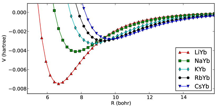
Figure 2: (color online). Electronic potential energy curves $V(R)$ from CCSD(T) calculations on the Alk-Yb systems.

System	$R_{e}$	$V(R_{e})$	$C_{6}$
	(bohr)	(${\rm mE}_{\rm h}$)	(${\rm E}_{\rm h}a_{0}^{6}$)
LiYb	6.65	$-7.48$	1594
NaYb	7.61	$-4.61$	1690
KYb	8.88	$-3.36$	2580
RbYb	9.28	$-2.99$	2830
CsYb	9.72	$-2.83$	3370

Table 1: Properties of the interaction potentials used in the present work. The well depths and equilibrium distances are from CCSD(T) calculations and the $C_{6}$ coefficients are from Eq. (11).

II.2.2 Hyperfine Coupling

The hyperfine coupling constant of an atom is a measure of the interaction between its nuclear spin and the electron spin density at the nucleus, which in the case of an alkali metal comes principally from the single valence electron. Approach of another atom perturbs the electronic wavefunction and alters the spin density at the nucleus, so that the coupling between the electron and nuclear spins becomes a function of internuclear distance $R$.

We have calculated the hyperfine coupling constants $\zeta_{a}(R)$ for the Alk-Yb systems, using density-functional theory with the KT2 functional Keal and Tozer (2003), as implemented in the ADF suite of programs ADF (2007). We fitted these results to a variety of functional forms and found that, in the range of $R$ for which the vibrational wavefunctions are non-zero, a Gaussian function $\Delta\zeta_{a}(R)=\zeta_{0}e^{-\beta(R-R_{c})^{2}}$ gave an adequate fit to the DFT results. These functions are shown in Figure 3 for each of the Alk-Yb systems and the parameters are given in Table 2.

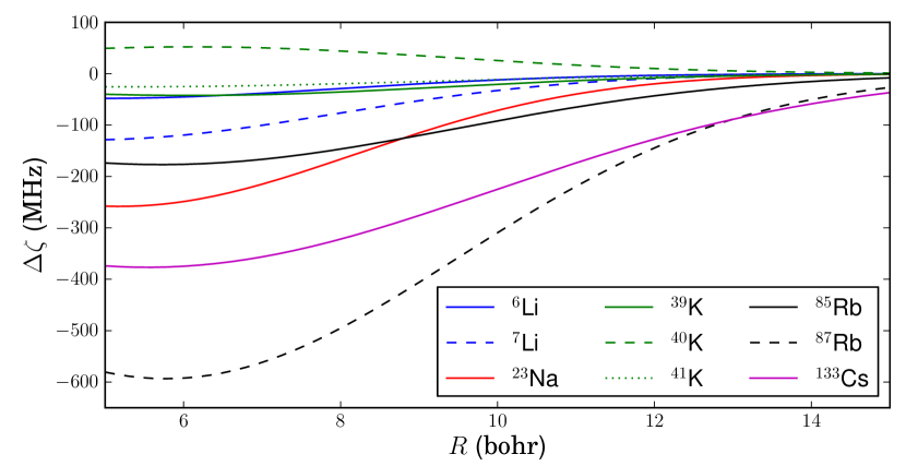
Figure 3: (color online). Distance dependence $\Delta\zeta_{a}(R)$ of the hyperfine coupling constants for the Alk-Yb systems.

	$\zeta_{0}$ (MHz)	$\beta$ (bohr${}^{-2})$	$R_{c}$ (bohr)
6Li	$-48.8$	0.0535	4.92
7Li	$-129.$	0.0535	4.92
23Na	$-258.$	0.0553	5.18
39K	$-42.4$	0.0474	6.09
40K	$52.5$	0.0474	6.09
41K	$-23.3$	0.0474	6.09
85Rb	$-177.$	0.0357	5.71
87Rb	$-597.$	0.0357	5.71
133Cs	$-377.$	0.0260	5.54

Table 2: Parameters of the Gaussian functions used to represent $\Delta\zeta_{a}(R)$, the distance-dependence of the hyperfine coupling constant of an alkali-metal atom interacting with Yb.

II.3 Resonance widths from coupled-channel calculations

Near resonance, the s-wave scattering length $a(B)$ as a function of magnetic field $B$ behaves as Moerdijk et al. (1995)

$$a(B)=a_{\rm bg}\left(1-\frac{\Delta}{B-B_{\rm res}}\right),$$ (12)

where $B_{\rm res}$ is the resonance position and $a_{\rm bg}$ is the background scattering length. The magnitude of the resonance width, $\Delta$, is critical for determining whether magnetoassociation is experimentally feasible. Defining $B_{\rm zero}$ as the field where $a(B)=0$ near resonance, Eq. (12) implies $\Delta=B_{\rm zero}-B_{\rm res}$.

In the present work, we obtained scattering lengths $a(B)$ principally from coupled-channel calculations. The coupled equations for each field $B$ were constructed in an uncoupled basis set $|s_{a}m_{s,a}\rangle|i_{a}m_{i,a}\rangle|LM_{L}\rangle$ and solved using the MOLSCAT package Hutson and Green (1994); González-Martínez and Hutson (2007). The s-wave scattering length was then obtained from the identity Hutson (2007) $a=(ik)^{-1}(1-S_{00})/(1+S_{00})$, where $S_{00}$ is the diagonal S-matrix element in the incoming channel, $k=\hbar^{-1}(2\mu E_{\rm col})^{1/2}$, and the collision energy $E_{\rm col}$ was taken to be 1 nK $\times{k_{\rm B}}$. MOLSCAT has an option to converge numerically on the fields corresponding to both poles and zeroes in $a(B)$, allowing the extraction of $\Delta$.

It should be noted that Eq. (12) characterizes the scattering length near resonance only for purely elastic scattering. If there exist lower-energy channels that allow decay, then $a(B)$ has a non-zero imaginary component and does not follow the simple pole formula (12) Hutson (2007). For $i_{b}=0$, the Hamiltonian (1) allows only elastic scattering even when the alkali-metal atom is in a magnetically excited state. However, when $i_{b}\neq 0$, couplings involving $\hat{i}_{b}\cdot\hat{s}$ can change $m_{f,a}$, and for alkali-metal atoms in magnetically excited states this provides additional couplings to lower-lying thresholds. We have previously described the behavior of $a(B)$ for resonances in such states for the LiYb systems Brue and Hutson (2012).

II.4 Resonance widths from Golden Rule

Coupled-channel calculations of resonance widths are straightforward but provide relatively little insight into the factors that affect resonance widths. We therefore develop here an alternative approach based on Fermi’s Golden Rule that allows us to understand the factors that determine the widths.

Fermi’s Golden Rule gives an expression for the width of a Feshbach resonance in terms of the off-diagonal matrix element of $\hat{H}^{\prime}$ (Eq. (8)) between the bound state $|\alpha_{2},m_{f,a},n\rangle$ (with vibrational quantum number $n$) and the continuum state $|\alpha_{1},m_{f,a},k\rangle$ (labeled by wavevector $k$, where $E_{\rm col}=\hbar^{2}k^{2}/2\mu$). The Breit-Wigner width in the energy domain, $\Gamma_{E}$, is

$$\Gamma_{E}(k)=2\pi\left|\middle<\alpha_{2},m_{f,a},n\middle|\hat{H}^{\prime}\middle|\alpha_{1},m_{f,a},k\middle>\right|^{2},$$ (13)

where the continuum function is normalized to a $\delta$-function of energy and has asymptotic amplitude $(2\mu/\pi\hbar^{2}k)^{1/2}$. At limitingly low collision energy, $\Gamma_{E}(k)$ behaves as Chin et al. (2010),

$$\Gamma_{E}(k)\xrightarrow{k\to 0}2ka_{\rm bg}\Gamma_{0}$$ (14)

where $a_{\rm bg}$ is the same background scattering length as in Eq. (12). $\Gamma_{0}$ is independent of energy and is related to the magnetic resonance width $\Delta$ of Eq. (12) by

$$\Delta=\frac{\Gamma_{0}}{\delta\mu_{\rm res}},$$ (15)

where $\delta\mu_{\rm res}$ is the difference between the magnetic moment of the molecular bound state and that of the free atom pair, which is simply the difference in slope of the crossing lines in Figure 1.

The expression for the magnetic resonance width $\Delta$ factorizes into spin-dependent and radial terms,

$$\Delta=\frac{\pi I_{m_{f,a}}(B)^{2}I_{nk}^{2}}{ka_{\rm bg}\delta\mu_{\rm res}},$$ (16)

where

$$I_{m_{f,a}}(B)=\left<\alpha_{2},m_{f,a}\right|\hat{i}_{a}\cdot\hat{s}\left|\alpha_{1},m_{f,a}\right>$$ (17)

and

$$I_{nk}=\int_{0}^{\infty}\psi_{n}(R)\Delta\zeta_{a}(R)\psi_{k}(R)\,{\rm d}R.$$ (18)

The quantity $I_{m_{f,a}}(B)$ is a purely atomic property, which arises because states $|\alpha_{i},m_{f,a}\rangle$ are eigenfunctions of $\hat{H}_{a}$. Pairs of states with the same $m_{f,a}$ are coupled through the operator $\Delta\zeta_{a}(R)\hat{i}_{a}\cdot\hat{s}$. At zero field, the states are eigenfunctions of $\hat{i}_{a}\cdot\hat{s}$, so that the perturbation has no off-diagonal matrix elements. At sufficiently high field, however, the states are well described by quantum numbers $m_{s,a}$ and $m_{i,a}$, such that for a given $m_{f,a}$ and $s_{a}=1/2$,

$$I_{m_{f,a}}(B)\xrightarrow{B\to\infty}\frac{1}{2}\left[i_{a}(i_{a}+1)-m_{f,a}^{2}+\textstyle{\frac{1}{4}}\right]^{\frac{1}{2}}.$$ (19)

The behavior of $I_{m_{f,a}}(B)$ between these two limits is shown as a function of magnetic field for ¹³³Cs in Figure 4. For positive $m_{f,a}$ the coupling increases monotonically before leveling off to the value (19), while for negative $m_{f,a}$ it increases with $B$, peaks, and then declines to the same value. At low fields, the coupling is approximately proportional to $B$, so that the resonance width is proportional to $B^{2}$ in this region. The range over which this behavior occurs is system-dependent; the coupling elements for lighter alkali metals level off at smaller $B$ than for Cs.

The factor $1/\delta\mu_{\rm res}$ in Eq.  (16) produces wider resonances when the difference in slope between the bound and continuum states at $B_{\rm res}$ is small. Particularly shallow crossings and wide resonances can occur when there is a “double crossing” involving a bound state that just dips below the threshold (as a function of $B$) before rising above it again. The magnetic fields at which this can occur are discussed in Section III.3 below.

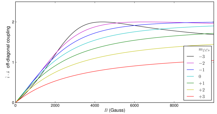
Figure 4: (color online). Off-diagonal matrix elements of $\hat{i}_{a}\cdot\hat{s}$ for ¹³³Cs between pairs of hyperfine states with the same value of $m_{f,a}$.

The bound and continuum functions, $\psi_{n}(R)$ and $\psi_{k}(R)$, are eigenfunctions that correspond to different eigenvalues of the 1-dimensional radial hamiltonian (9). They are thus orthogonal to one another, and the matrix element $I_{nk}$ of Eq. (18) is non-zero only because of the $R$-dependence of $\Delta\zeta_{a}(R)$.

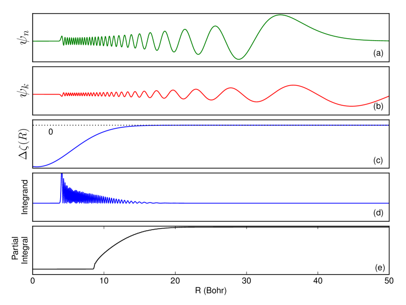
Figure 5: (color online). The functions contributing to the integral $I_{nk}$ of Eq. (18) for CsYb. (a) Wavefunction for the $n=-4$ bound state, $\psi_{n=-4}(R)$, which is the shallowest bound state for which crossings exist. (b) wavefunction for the low-energy continuum state, $\psi_{k}(R)$. (c) $\Delta\zeta_{\rm Cs}(R)$. (d) the integrand of the matrix element, $\psi_{n}\psi_{k}\Delta\zeta$. (e) The partial integral $\int_{0}^{R}\psi_{n}(R^{\prime})\psi_{k}(R^{\prime})\Delta\zeta(R^{\prime}){\rm d}R^{\prime}$.

Figure 5 shows how the integral $I_{nk}$ develops as a function of $R$ in a typical case. The upper three panels show $\psi_{n}(R)$, $\psi_{k}(R)$ and $\Delta\zeta_{a}(R)$. Figure 5(d) shows the integrand of Eq. (18), which is the product of the three. For weakly bound states, the bound and continuum functions remain almost in phase with one another across the width of the potential well, so that their product always maintains the same sign. The integral thus accumulates monotonically as shown in the bottom panel. Its value depends principally on $\Delta\zeta_{a}(R)$ between the inner turning point and the potential minimum. Deeply bound states lose phase with the continuum at shorter ranges; in principle this produces some cancelation that reduces the value of the integral, but the effect of this is small for the near-dissociation levels considered here.

Further insight may be gained by considering the integral $I_{nk}$ semiclassically. In the WKB (Wentzel-Kramers-Brillouin) approximation, the bound and continuum wavefunctions both oscillate with amplitudes proportional to $k(R)^{-1/2}$ in the classically allowed region, where $k(R)=[2\mu(E-V(R))/\hbar^{2}]^{1/2}$. For very weakly bound states and low collision energies, $E$ may be neglected, so

$$I_{nk}\propto\int_{r_{\rm in}}^{\infty}k(R)^{-1}\Delta\zeta(R)\,{\rm d}R,$$ (20)

where $r_{\rm in}$ is the inner classical turning point at $E=0$. This structure is clearly visible in Figure 5(d).

Near threshold, the WKB approximation gives an incorrect ratio between the short-range and long-range amplitudes of a scattering wavefunction. Quantum Defect Theory (QDT) Mies (1984) corrects for this using an energy-dependent function $C(k)$, which is 1 far from threshold but is given by

$$C(k)^{-2}=k\bar{a}\left[1+\left(1-\frac{a_{\rm bg}}{\bar{a}}\right)^{2}\right]$$ (21)

at limitingly low energy Chin et al. (2010). The correction amplifies the short-range wavefunction by a factor $C(k)^{-1}$, which has a minimum value of $(k\bar{a})^{1/2}$ when $a_{\rm bg}=\bar{a}$ but is approximately $(k/\bar{a})^{1/2}a_{\rm bg}$ when $|a_{\rm bg}|\gg\bar{a}$.

Combining all these effects gives a semiclassical expression for the Golden Rule width,

$$\Delta = \frac{\mu}{\hbar^{2}}\frac{\bar{a}}{a_{\rm bg}}\left[1+\left(1-\frac{a_{\rm bg}}{\bar{a}}\right)^{2}\right]\frac{[I_{m_{f,a}}(B)]^{2}}{N\delta\mu_{\rm res}}$$ (22)

$$\times \left[\int_{r_{\rm in}}^{\infty}k(R)^{-1}\Delta\zeta(R)\,{\rm d}R\right]^{2},$$

where $N$ is the normalization integral for the WKB bound-state wavefunction,

$$N=\frac{1}{2}\int_{R_{\rm in}}^{R_{\rm out}}k(R)^{-1}\,dR,$$ (23)

which is taken between the classical turning points $R_{\rm in}$ and $R_{\rm out}$ at energy $E_{n}$. Eq. (22) completely avoids the calculation of any quantal wavefunctions and gives results within 2% of the quantal Golden Rule width (16).

The semiclassical approach may be taken one step further, with a small approximation. For a near-dissociation vibrational state with an interaction potential that varies as $-C_{j}R^{-j}$ at long range, Le Roy and Bernstein Le Roy and Bernstein (1970) have shown that the integral (23) is

$$\int_{R_{\rm in}}^{R_{\rm out}}k(R)^{-1}\,dR\approx\left(\frac{\pi\hbar^{2}}{2\mu}\right)^{\frac{1}{2}}\frac{\Gamma\left(\frac{1}{2}+\frac{1}{j}\right)}{\Gamma\left(1+\frac{1}{j}\right)}\frac{C_{j}^{1/j}}{j}|E_{n}|^{-\frac{j+2}{2j}},$$ (24)

where $\Gamma(x)$ is the gamma function. For the present case, with $R^{-6}$, $\Delta$ is thus proportional to $|E_{n}|^{2/3}$. Deeper bound states thus produce broader resonances, though generally at higher magnetic field. For the bound states of interest here, Eq. (24) is accurate to within 6%.

As described below, different isotopes of Yb offer different values of the scattering length $a_{\rm bg}$. Eq. (22) shows that large values of $\Delta$ may occur when $|a_{\rm bg}|$ is either very large or very small: $\Delta$ is directly proportional to $a_{\rm bg}$ when $|a_{\rm bg}|\gg\bar{a}$, and inversely proportional to $a_{\rm bg}$ when $|a_{\rm bg}|\ll\bar{a}$.

Overall the Golden Rule approximation (22) produces resonance widths that agree within 2% with those from full coupled-channel calculations. It also produces important insights into the origins of the widths, and makes it much easier to select systems and isotopic combinations with experimentally desirable properties.

II.5 Sensitivity to the interaction potential

The Feshbach resonance positions and widths are strongly dependent on the s-wave scattering length of the system. The background scattering length $a_{\rm bg}$, the binding energies of high-lying vibrational levels $E_{n}$, and the non-integer quantum number at dissociation $v_{\rm D}$ can all be related to a semiclassical phase integral $\Phi(E)$,

$$\Phi(E)=\int_{R_{\rm in}}^{R_{\rm out}}k(R)\,{\rm d}R.$$ (25)

For a potential with long-range behavior $V(R)=-C_{6}R^{-6}$, the scattering length is

$$a_{\rm bg}=\bar{a}\left[1-\tan\left(\Phi(0)-\frac{\pi}{8}\right)\right]$$ (26)

where $\bar{a}$ is the mean scattering length of Gribakin and Flambaum Gribakin and Flambaum (1993), which is proportional to $(\mu C_{6})^{1/4}$. Values for $\bar{a}$ for all the alkali metals with Yb atoms are given for representative isotopes in Table 3. The non-integer quantum number at dissociation is

$$v_{\rm D}^{\rm GF}=\frac{\Phi(0)}{\pi}-\frac{5}{8},$$ (27)

where the superscript GF distinguishes the Gribakin-Flambaum value from the (less accurate) first-order WKB value (see section III.3). It should be noted that $a_{\rm bg}$ is a single-valued function of the fractional part of $v_{\rm D}^{\rm GF}$ and is independent of its integer part.

	168Yb	176Yb
6Li	36.29	36.31
7Li	37.66	37.68
23Na	50.50	50.57
40K	63.10	63.24
87Rb	74.52	74.82
133Cs	83.05	83.48

Table 3: Mean scattering lengths $\bar{a}$ (in bohr) for the Alk-Yb systems.

Potential energy curves from electronic structure calculations for heavy molecules are typically accurate to at best a few percent. For curves that support 35 to 70 bound states, such as those for the systems considered here, this uncertainty is enough to span more than 1 in $v_{\rm D}$. It is thus not possible to predict $a_{\rm bg}$ for these systems from electronic structure calculations alone. An experimental measurement is essential to limit the possible range of $a_{\rm bg}$.

If the uncertainty in $v_{\rm D}$ is much greater than 1 and we assume that the possible values of $\Phi(0)$ (and hence $v_{\rm D}$) are uniformly distributed over such a range of uncertainty in $V(r)$, we find from Eq. (26) that there is a 50% probability that $a_{\rm bg}$ is in the range $[0,2\bar{a}]$, and a 70.5% probability that it is in the range $[-\bar{a},3\bar{a}]$.

Different isotopologues of the same molecule have different reduced masses $\mu$. Since $k(R)$ is proportional to $\mu^{1/2}$, changing between different isotopes of Yb alters $\Phi(0)$, and hence $v_{\rm D}$ and $a_{\rm bg}$, in a very well-defined way, which depends only weakly on the potential well depth. For the case of LiYb, changing the heavy-atom isotope has very little effect on the reduced mass and therefore on $a_{\rm bg}$. For the heavier alkalis, by contrast, changing the Yb isotope allows the scattering length to be tuned over a wide range. Table 4 summarizes the number of bound states and the amount by which it may be tuned for all the alkali-metal + Yb systems.

	$v_{\rm D}$(172Yb)	$\Delta v_{\rm D}$(Yb)
6Li	23	0.02
7Li	25	0.02
23Na	35	0.10
40K	45	0.20
87Rb	62	0.49
133Cs	69	0.70

Table 4: The integer part of $v_{\rm D}$ for Alk-Yb systems, based on the potential curves from CCSD(T) calculations, together with the amount $\Delta v_{\rm D}$ by which $v_{\rm D}$ may be tuned by varying the isotope of Yb. Note that the number of bound states is $v_{\rm D}+1$.

III Results and Discussion

We have previously calculated resonance positions and widths for the LiYb systems Brue and Hutson (2012), using estimates of $a_{\rm bg}$ obtained from thermalization measurements for ⁶Li¹⁷⁴Yb Hara et al. (2011); Ivanov et al. (2011). In the following subsections, we present calculations of resonance positions and widths for two cases representative of the heavier alkali metals: RbYb, where the scattering lengths are approximately known, and CsYb, where the scattering lengths have yet to be measured.

III.1 RbYb

Interactions of RbYb mixtures have been studied by Görlitz and coworkers Baumer et al. (2011); Baumer (2010); Münchow et al. (2011); Münchow (2012). Baumer et al. Baumer et al. (2011); Baumer (2010) measured thermalization rates and density profiles for mixtures of ⁸⁷Rb with a variety of Yb isotopes, and interpreted the results in terms of background scattering lengths. In particular, ⁸⁷Rb¹⁷⁴Yb was found to have an extremely large scattering length, which produced phase separation of the atomic clouds, while ⁸⁷Rb¹⁷⁰Yb was found to have an extremely small one. Münchow et al. Münchow et al. (2011); Münchow (2012) measured 2-photon photoassociation spectra of high-lying vibrational states of the electronic ground state: for ⁸⁷Rb¹⁷⁶Yb, 6 states were observed with binding energies between about 300 MHz and 60 GHz Münchow et al. (2011); Münchow (2012), whereas for each of ¹⁷⁰Yb, ¹⁷²Yb and ¹⁷⁴Yb, two states were observed with binding energies between 100 and 1500 MHz. Münchow Münchow (2012) fitted the binding energies to a Lennard-Jones potential model and inferred from the mass scaling that the potential supports about 66 bound states for ⁸⁷Rb¹⁷⁴Yb and ⁸⁷Rb¹⁷⁶Yb, with one fewer state for lighter Yb isotopes. The presence of a bound state very close to dissociation in ⁸⁷Rb¹⁷⁴Yb produces its large positive scattering length.

The Lennard-Jones potential reproduces the experimental spectra satisfactorily, but the mass scaling determines only the number of bound states and there is no reason to expect the potential to have the correct well depth, equilibrium distance, or inner turning point. These features are however important in the calculation of resonance widths. We have therefore refitted the binding energies measured by Münchow Münchow (2012), together with the scattering length for ⁸⁷Rb¹⁷⁰Yb, to obtain a new potential curve based on our CCSD(T) results described above. Our best fit was obtained by multiplying the CCSD(T) potential by a scaling factor $\lambda_{\rm scl}=1.09581$ and adjusting $C_{6}$ to 2874.7 $E_{\rm h}a_{0}^{6}$, producing a potential that supports 66 bound states for ⁸⁷Rb¹⁷⁶Yb. We also introduced long-range $C_{8}$ and $C_{10}$ coefficients related to $C_{6}$ by a ratio $\gamma=C_{8}/C_{6}=C_{10}/C_{8}$, with an optimum value $\gamma=267.5$ bohr² for the potential above. Since the resulting long-range potential is valid to shorter distances than the pure $C_{6}R^{-6}$ potential used for the other systems, the switching function Janssen et al. (2009) was applied between 20 and 30 bohr in this case. It should be noted that adequate fits could also be obtained with one or two additional (or fewer) bound states: increasing $\lambda_{\rm scl}$ by 0.036 and $C_{6}$ by $37\ E_{\rm h}a_{0}^{6}$ produces a potential with one extra bound state at the bottom of the well but the high-lying states almost unchanged.

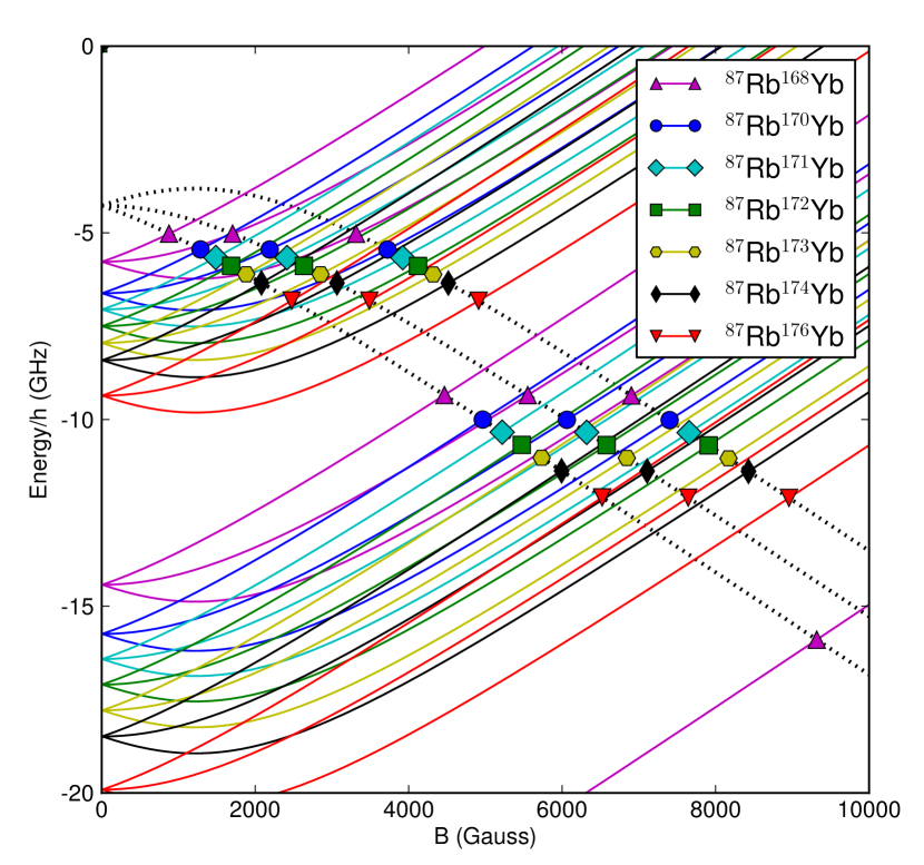
Figure 6: (color online). Resonance crossings for ⁸⁷Rb with the stable isotopes of Yb, demonstrating the mass-scaling effect. The threshold levels for $m_{f,{\rm Rb}}=-1,0,+1$ sublevels of the $f=1$ manifold are shown as dotted black lines, while the molecular bound state $m_{f,{\rm Rb}}=-1,0,+1$ sublevels for the $f=2$ manifolds are shown in different colors for the different isotopes of Yb. The bound states for $m_{f,{\rm Rb}}=-2$ and +2 are not shown. The highest bound state shown here is the $n=-4$ vibrational state for the combinations of ⁸⁷Rb with ¹⁶⁸Yb$\to^{173}$Yb, and $n=-5$ for ⁸⁷Rb¹⁷⁴Yb and ⁸⁷Rb¹⁷⁶Yb.

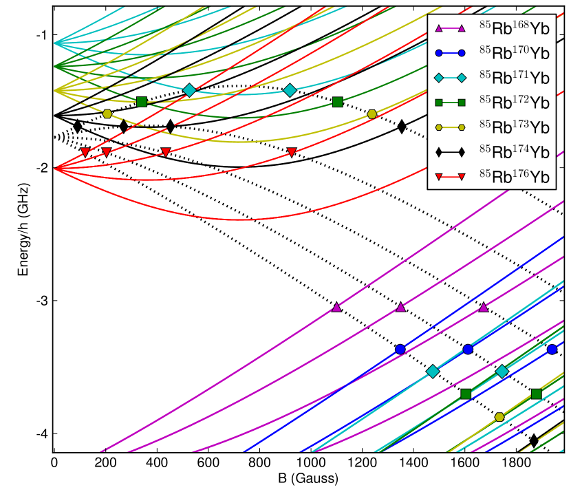
Figure 7: (color online). Resonance crossings for ⁸⁵Rb with the stable isotopes of Yb. The threshold levels for $m_{f,{\rm Rb}}=-2,-1,0,+1,+2$ sublevels of the $f=2$ manifold are shown as dotted black lines, while the corresponding molecular bound-state sublevels for the $f=3$ manifolds are shown in different colors for the different isotopes of Yb. The bound states for $m_{f,{\rm Rb}}=-3$ and +3 are not shown. The highest bound state shown here is the $n=-3$ vibrational state.

Rb-Yb	$m_{f,{\rm Rb}}$	$B_{\rm res}$	$\Delta$	$a_{\rm bg}$	$\frac{|\Delta|}{B_{\rm res}}$	$s_{\rm res}$
		(G)	(mG)	(bohr)	(ppm)
87-168	$-1$	3314	4.6	39	1.4	$8.4\times 10^{-4}$
	0	1705	2.0	39	1.1	$3.0\times 10^{-4}$
	1	877	0.3	39	0.4	$5.9\times 10^{-5}$
	1	4466	2.4	39	0.5	$5.9\times 10^{-4}$
87-170	$-1$	3723	$-31.1$	$-11$	8.3	$1.8\times 10^{-3}$
	0	2189	$-16.6$	$-11$	7.5	$8.2\times 10^{-4}$
	1	1287	$-3.8$	$-11$	2.9	$2.1\times 10^{-4}$
	1	4965	$-17.9$	$-11$	3.6	$1.3\times 10^{-3}$
87-171	$-1$	3923	$-10.9$	$-58$	2.7	$3.4\times 10^{-3}$
	0	2415	$-6.2$	$-58$	2.5	$1.7\times 10^{-4}$
	1	1487	$-1.6$	$-58$	1.0	$4.8\times 10^{-4}$
87-172	$-1$	4122	$-10.4$	$-156$	2.5	$8.9\times 10^{-3}$
	0	2636	$-6.2$	$-156$	2.3	$4.8\times 10^{-3}$
	1	1686	$-1.7$	$-155$	1.0	$1.5\times 10^{-3}$
87-173	$-1$	4320	$-20.7$	$-576$	4.7	$6.7\times 10^{-2}$
	0	2852	$-13.0$	$-571$	4.5	$3.8\times 10^{-2}$
	1	1883	$-3.9$	$-569$	2.0	$1.3\times 10^{-2}$
87-174	$-1$	4517	23.9	991	5.2	$1.4\times 10^{-1}$
	0	3066	16.0	1000	5.2	$8.5\times 10^{-2}$
	1	2081	5.2	1005	2.5	$3.0\times 10^{-2}$
87-176	$-1$	4912	3.5	224	0.7	$4.7\times 10^{-3}$
	0	3488	2.5	224	0.7	$3.2\times 10^{-3}$
	1	2476	0.9	224	0.4	$1.2\times 10^{-3}$

Table 5: Predicted positions and widths for resonances with $\Delta m_{f,{\rm Rb}}=0$ for ⁸⁷RbYb systems at fields $B_{\rm res}<5000$ G.

Rb-Yb	$m_{f,{\rm Rb}}$	$B_{\rm res}$	$\Delta$	$a_{\rm bg}$	$\frac{|\Delta|}{B_{\rm res}}$	$s_{\rm res}$
		(G)	(mG)	(bohr)	(ppm)
85-168	$1$	1350	0.17	219	0.12	$2.1\times 10^{-4}$
	$2$	1100	0.066	219	0.06	$8.8\times 10^{-5}$
85-170	$2$	1348	0.048	137	0.04	$4.1\times 10^{-5}$
85-171	$-2$	526	$-0.10$	116	0.18	$1.7\times 10^{-5}$
	$-2$	918	0.30	116	0.32	$5.4\times 10^{-4}$
	$2$	1475	0.048	116	0.03	$4.1\times 10^{-5}$
85-172	$-2$	340	$-0.019$	99	0.06	$5.4\times 10^{-6}$
	$-2$	1104	0.21	99	0.19	$6.1\times 10^{-5}$
85-173	$-2$	206	$-0.0055$	84	0.03	$1.5\times 10^{-6}$
	$-2$	1238	0.21	84	0.17	$6.4\times 10^{-5}$
85-174	$-2$	90	$-0.0009$	70	0.01	$2.9\times 10^{-7}$
	$-2$	1354	0.24	69	0.18	$7.0\times 10^{-5}$
	$-1$	270	$-0.11$	70	0.39	$4.4\times 10^{-6}$
	$-1$	452	0.30	69	0.18	$1.2\times 10^{-5}$
85-176	$-1$	925	0.43	39	0.46	$5.5\times 10^{-5}$
	0	434	0.14	39	0.32	$1.4\times 10^{-5}$
	1	203	0.021	39	0.10	$2.7\times 10^{-6}$
	2	120	0.0033	39	0.03	$5.7\times 10^{-7}$

Table 6: Predicted positions and widths for resonances with $\Delta m_{f,{\rm Rb}}=0$ for ⁸⁵RbYb systems at fields $B_{\rm res}<1500$ G.

We have carried out coupled-channel calculations for the RbYb systems using the fitted potential with 66 bound states. For the fermionic isotopes ¹⁷¹Yb and ¹⁷³Yb, we neglected couplings due to $\Delta\zeta_{\rm Yb}$. The crossings responsible for the resonances for ⁸⁷RbYb are shown in Figure 6 and the resonance positions and widths are given in Table 5 for all resonances located below 5000 G. The corresponding results for ⁸⁵RbYb are given in Figure 7 and Table 6 for resonances located below 1500 G. A full listing of all resonances below 10000 G is provided as Supplemental Material Sup . The resonance positions are generally within about 50 G of those obtained by Münchow Münchow (2012) with a Lennard-Jones model of the potential.

The pattern of widths for ⁸⁷RbYb closely follows expectations from Eq. (22). Only ⁸⁷Rb¹⁶⁸Yb has a resonance below 1000 G, and that has a very low width (300 $\mu$G), in part because of dropoff in $I_{m_{f,{\rm Rb}}}(B)$ at low fields. Nevertheless, resonances with calculated widths as narrow as 0.2 $\mu$G have been observed as 3-body loss features in Na Knoop et al. (2011), and resonances a few mG wide have been observed in LiNa at fields as high as 2050 G Schuster et al. (2012). ⁸⁷Rb¹⁷⁰Yb has particularly large widths as measured by $\Delta$ (up to 30 mG), but this is simply because $a_{\rm bg}$ is small in this case: the quantity $a_{\rm bg}\Delta$, which is a better measure of the suitability of a resonance for magnetoassociation Julienne et al. (2004); Góral et al. (2004), is not particularly large for this isotopologue. By contrast, ⁸⁷Rb¹⁷³Yb and ⁸⁷Rb¹⁷⁴Yb, which both have $|a_{\rm bg}|\gg\bar{a}$, have resonances up to 25 mG wide. Experimentally, ⁸⁷Rb¹⁷⁴Yb displays phase separation that will inhibit molecule formation even for low-temperature thermal clouds Baumer et al. (2011), but ⁸⁷Rb¹⁷³Yb does not Baumer (2010), and is a good candidate for magnetoassociation if the high fields in Table 5 can be achieved.

For ⁸⁵RbYb, there are no resonances with $\Delta/B_{\rm res}>10^{-7}$. This arises mostly because of the lower hyperfine coupling constant $\zeta$ for ⁸⁵Rb, which both reduces the magnitude of $\Delta\zeta(R)$ and further reduces the widths through the factor of $|E_{n}|^{2/3}$ described following Eq. (24) above. However, there are several resonances predicted below 1500 G, as shown in Table 6, and some of the broader ones (still below 1 mG width) may be suitable for molecule formation. In particular, our best-fit potential predicts a pair of resonances for $m_{f,{\rm Rb}}=-1$ for ⁸⁵Rb¹⁷⁴Yb, where the atomic and molecular states just intersect and undergo a double crossing as shown in Fig. 7. The precise positions and widths of these resonances are very sensitive to the potential details, and indeed Münchow’s Lennard-Jones model predicted that the atomic and molecular states just miss each other instead of just crossing Münchow (2012).

Tables 5 and 6 include only resonances driven by $\Delta\zeta(R)$ for Rb, which conserve $m_{f,\rm Rb}$. If the Yb isotope has nuclear spin, as for fermionic ¹⁷¹Yb and ¹⁷³Yb, additional resonances can occur at crossings with $\Delta m_{f,\rm Rb}=\pm 1$, driven by $\Delta\zeta(R)$ for Yb Brue and Hutson (2012). In particular, ⁸⁷Rb¹⁷¹Yb has a lower-field and therefore potentially more accessible group of resonances near 1210 G, where the molecular states with $m_{f,{\rm Rb}}=+2$ and $m_{i,{\rm Yb}}$ (not shown in Fig. 6) cross the thresholds with $m_{f,{\rm Rb}}=+1$ and $m_{i,{\rm Yb}}-1$.

All the resonances in Tables 5 and 6 are strongly closed-channel-dominated. This may be quantified using the dimensionless resonance parameter $s_{\rm res}=(a_{\rm bg}/\bar{a})(\delta\mu\Delta/\bar{E})$, where $\bar{E}=\hbar^{2}/(2\mu\bar{a}^{2})$. It may be seen that $s_{\rm res}$ is never greater than 0.2, and approaches such values only when $|a_{\rm bg}|$ is very large. In some cases $s_{\rm res}$ can be less than $10^{-6}$.

Molecule formation by magnetoassociation is usually carried out by preparing the atomic mixture close to a resonance, on the side where the atomic state lies below the molecular state, and then ramping the field over the resonance. However, for narrow resonances in Cs₂ (a few mG wide, at low fields), Mark et al. Mark et al. (2007) found it effective simply to hold the field on resonance for a few milliseconds. Nevertheless, the most efficient molecule production occurs with a field ramp that is slow enough to cross the resonance adiabatically Julienne et al. (2004); Góral et al. (2004); Hodby et al. (2005). Small field inhomogeneities are not a big problem, as they will simply cause different parts of the cloud to cross the resonance at slightly different times. However, field noise is potentially a problem, particularly high-frequency noise that causes nonadiabatic crossings through the resonance. It will therefore be important to design a molecule creation experiment with very careful field control. In this context it is worth noting that Zürn et al. Zürn et al. (2013) have recently carried out radiofrequency spectroscopy on Li₂ molecules at fields around 800 G with a field precision of $\pm 1$ mG, which is close to 1 part in $10^{6}$, while Heo et al. Heo et al. (2012) achieved molecule formation in ⁶LiNa, using a resonance 10 mG wide at 745 G, with active feedback stabilization of the current to achieve field noise less than 10 mG Heo et al. (2012).

III.2 CsYb

Cesium possesses several properties that make it favorable compared to the other alkali-metal elements for magnetoassociation with Yb. It has the highest mass of the alkali metals, which leads to greater mass scaling through changing the isotope of the closed-shell atom. Its larger mass also provides a higher density of bound states near threshold and thus offers better chances of resonances at low magnetic field. Additionally, its relatively large nuclear spin allows larger off-diagonal $\hat{i}_{a}\cdot\hat{s}$ elements. Finally, the effects of $\Delta\zeta(R)$ are larger for Cs than for most of the other alkali metals.

The CsYb potential shown in Fig. 2 supports 70 bound states for all Yb isotopes, and has a background scattering length $a_{\rm bg}=-38$ bohr for ¹³³Cs¹⁷⁴Yb. However, the electronic structure calculations have a degree of inaccuracy, and a plausible change of $\pm 10$% in the well depth would produce a change of $\pm 3$ in $v_{\rm D}$. Since the scattering length depends on the fractional part of $v_{\rm D}$, it cannot be predicted from these calculations. However, altering the Yb isotopic mass across its possible range from 168 to 176 changes $v_{\rm D}$ by about 0.70, so that a wide range of background scattering lengths will be accessible by varying the Yb isotope. We have therefore carried out calculations for CsYb as a function of $a_{\rm bg}$.

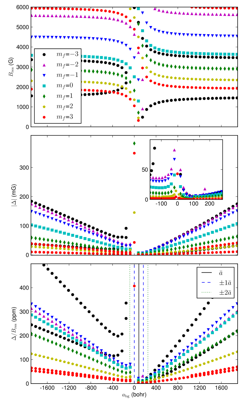
Figure 8: (color online). Resonance positions and widths for ¹³³Cs¹⁷⁴Yb, obtained from coupled-channel calculations, as a function of the background scattering length $a_{\rm bg}$. Top panel: Resonance position $B_{\rm res}$. Center panel: Width $|\Delta|$, with an inset showing an expanded view for values of $a_{\rm bg}$ near the mean scattering length, $\bar{a}$. Bottom panel: $\Delta/B_{\rm res}$ in parts per million.

The top panel of Figure 8 shows the resonance positions and widths for ¹³³Cs¹⁷⁴Yb as a function of $a_{\rm bg}$. The plot would be almost identical for any other Yb isotope (though different isotopes will have different scattering lengths). There are multiple resonances for each value of $m_{f,{\rm Cs}}$, which occur when bound states $|\alpha_{2},m_{f,{\rm Cs}},n\rangle$ cross the scattering threshold $|\alpha_{1},m_{f,{\rm Cs}}\rangle$. As $a_{\rm bg}$ increases, the binding energies decrease and the most of the crossings (those with positive $\delta\mu$) shift to lower magnetic fields. In the $m_{f,{\rm Cs}}=+3$ case, the position of one resonance changes from $B\approx 6000$ G to $B\approx 2000$ G as $a_{\rm bg}$ increases from $-2000$ to $+2000$ bohr. When a state becomes too shallow to cross the lower threshold at all, the corresponding resonance line either disappears through $B=0$ or (in the case of a double crossing, as for $m_{f,{\rm Cs}}=-3$) reaches a maximum $a_{\rm bg}$ where the two crossings coalesce.

The middle panel of Figure 8 shows $|\Delta|$ as a function of $a_{\rm bg}$. The spikes in $|\Delta|$ near $a_{\rm bg}=0$ occur because of the $a_{\rm bg}$ in the denominator of Eq. (22). However, the strength of the peak in $a(B)$ [Eq. (12)] is actually $a_{\rm bg}\Delta$ rather than $\Delta$ itself, so this situation does not offer particular advantages for molecule formation. For $|a_{\rm bg}\gg\bar{a}$, the widths vary linearly with $a_{\rm bg}$ as described in Section II.4. A particularly interesting feature of this plot is the spike in the $m_{f,{\rm Cs}}=-3$ widths near $a_{\rm bg}=-100$ bohr, which is physically significant. As noted above, the bound states for this magnetic sublevel experience a double crossing with the lower threshold in this region; as the two crossings approach one another, $\delta\mu_{\rm res}$ decreases and $\Delta$ increases as given by Eq. (16). A similar spike occurs in the $m_{f,{\rm Cs}}=-2$ resonance widths near 167 bohr. The inset shows an expanded view of $|\Delta|$ for the range of $a_{\rm bg}$ from $-\bar{a}$ to $3\bar{a}$; as described in section II.5, there is about a 70% probability that $a_{\rm bg}$ lies in this range for any particular isotope.

III.3 Choosing promising systems

The Fermi Golden Rule treatment developed above shows that the most important properties leading to large resonance widths are a large magnitude of the background scattering length and the occurrence of “double crossings” where the bound and continuum states have similar (small) magnetic moments. It is instructive to consider the conditions where these two enhancements can occur together.

At zero field, the hyperfine splitting of an alkali-metal atom in a ²S state is $E_{\rm hf}(0)=\zeta\left(i+\frac{1}{2}\right)$. As a function of magnetic field, the splitting between two states with the same value of $m_{f}$ (neglecting the nuclear Zeeman term) is

$$E_{\rm hf}(B)=\left[E_{\rm hf}(0)^{2}+\frac{4m_{f}E_{\rm hf}(0)}{2i+1}g_{e}\mu_{\rm B}B+(g_{e}\mu_{\rm B}B)^{2}\right]^{\frac{1}{2}}.$$ (28)

For negative values of $m_{f}$, this has a minimum value

$$E_{m_{f}}^{\rm close}=E_{\rm hf}(0)\left(1-\frac{4m_{f}^{2}}{(2i+1)^{2}}\right)^{\frac{1}{2}}$$ (29)

at a field

$$B_{m_{f}}^{\rm close}=\frac{-2m_{f}E_{\rm hf}(0)}{(2i+1)g_{e}\mu_{\rm B}}=\frac{-m_{f}\zeta}{g_{e}\mu_{\rm B}}.$$ (30)

The first-order WKB quantisation formula, expressed in terms of the phase integral of Eq. (25), is

$$\Phi(E)=\left(v+\frac{1}{2}\right)\pi.$$ (31)

Le Roy and Bernstein Le Roy and Bernstein (1970) showed that this implies that, for a long-range potential $V(R)=-C_{j}R^{-j}$ with $j>2$, near-dissociation levels exist at energies

$$E_{v}=-[H_{j}(v_{\rm D}^{\rm WKB}-v)]^{2j/(j-2)},$$ (32)

where

$$H_{j}=\left(\frac{\pi\hbar^{2}}{2\mu}\right)^{\frac{1}{2}}\frac{(j-2)}{C_{j}^{1/j}}\frac{\Gamma\left(1+\frac{1}{j}\right)}{\Gamma\left(\frac{1}{2}+\frac{1}{j}\right)}.$$ (33)

However, Eqs. (31) and (32) do not take account of the Gribakin-Flambaum correction Gribakin and Flambaum (1993), which replaces the $(v+\frac{1}{2})$ in Eq. (31) with $(v+\frac{1}{2}+\epsilon(v))$, where $\epsilon(v)$ is zero for deeply bound levels but is $\frac{1}{8}$ at dissociation for a long-range $R^{-6}$ potential. This correction may have a significant effect on the energy of the least-bound level Boisseau et al. (1998, 2000), which is responsible for the Feshbach resonances Li-Yb Brue and Hutson (2012) but is small for the slightly deeper levels that are responsible for the resonances in the heavier Alk-Yb systems. As a result, the near-dissociation levels (except $n=-1$) actually occur at energies close to

$$E_{v}=-H_{6}^{3}\left(v_{\rm D}^{\rm WKB}-v\right)^{3}=-H_{6}^{3}\left(v_{\rm D}^{\rm GF}-v+\frac{1}{8}\right)^{3},$$ (34)

where

$$v_{\rm D}^{\rm WKB}=\frac{\Phi(0)}{\pi}-\frac{1}{2}=v_{\rm D}^{\rm GF}+\frac{1}{8}$$ (35)

when expressed in terms of $v_{\rm D}^{\rm GF}$ from Eq. (27).

Very large values of $|a_{\rm bg}|$ correspond to near-integer values of $v_{\rm D}^{\rm GF}$, so the condition for a very large value of $|a_{\rm bg}|$ to coexist with a “double crossing” near $B_{m_{f}}^{\rm close}$ is that the dimensionless quantity

$$X_{m_{f}}=\left[\frac{E_{\rm hf}(0)}{H_{6}^{3}}\left(1-\frac{4m_{f}^{2}}{(2i+1)^{2}}\right)^{\frac{1}{2}}\right]^{1/3}-\frac{1}{8}$$ (36)

should be approximately an integer. The quantity $X_{m_{f}}$ may be interpreted as the vibrational quantum number (relative to threshold) that will just give a double crossing between a molecular state associated with the upper hyperfine level and an atomic state at the lower hyperfine threshold with the same $m_{f}$. It depends strongly on the alkali-metal isotope through the nuclear spin and hyperfine splitting, but is only very weakly dependent on the Yb isotope chosen. It is proportional to $C_{6}^{1/2}$ (through $H_{6}$), but is otherwise completely independent of the interaction potential. Values of $X_{m_{f}}$ slightly smaller than than an integer allow a very large value of $|a_{\rm bg}|$ to coexist with a double crossing further from $B_{m_{f}}^{\rm close}$, or a large negative value of $a_{\rm bg}$ to coexist with a double crossing near $B_{m_{f}}^{\rm close}$. In general, large negative values of $a_{\rm bg}$ may be more favorable for molecule formation than large positive ones, because negative values will not cause phase separation in condensates.

	$m_{f}$	$B_{m_{f}}^{\rm close}$ (G)	$X_{m_{f}}$	$a^{\max}_{m_{f}}$ (bohr)	$a^{\rm min}$ (bohr)
6Li	$-1/2$	27	0.20	86	84
7Li	$-1$	143	0.40	51	47
23Na	$-1$	316	1.06	297	175
39K	$-1$	82	0.90	$-122$	$-302$
40K	$-7/2$	357	1.17	173	87
40K	$-5/2$	255	1.29	111	87
40K	$-3/2$	153	1.35	94	87
40K	$-1/2$	51	1.38	88	87
41K	$-1$	45	0.71	14	$-1$
85Rb	$-2$	722	2.36	111	48
85Rb	$-1$	361	2.56	61	48
87Rb	$-1$	1219	3.32	123	78
133Cs	$-3$	2460	3.95	$-399$	71
133Cs	$-2$	1640	4.33	133	71
133Cs	$-1$	820	4.50	84	71

Table 7: The quantity $X_{m_{f}}$ of Eq. (36), which needs to be close to an integer for double crossings to exist for large values of $|a_{\rm bg}|$, together with the range of scattering lengths for which double crossings can exist for a pure $R^{-6}$ potential. The values are almost independent of the Yb isotope.

Values of $X_{m_{f}}$ for all the Alk-Yb systems are given in Table 7. They may be converted into values of the scattering length that just cause double crossings (for a pure $C_{6}/R^{6}$ potential) using

$$a^{\rm max}_{m_{f}}=\bar{a}\left\{1-\tan\left[\pi\left(X_{m_{f}}+\textstyle{\frac{1}{2}}\right)\right]\right\}.$$ (37)

Scattering lengths between $a^{\rm max}_{m_{f}}$ and $a^{\rm min}=a^{\rm max}_{0}$ will give rise to double crossings (where values of $a^{\rm min}>a^{\rm max}_{m_{f}}$ are to be interpreted as allowing the scattering length to be decreased from $a^{\rm max}_{m_{f}}$, through a pole and back down from $+\infty$ to $a^{\rm min}$). However, only values close to $a^{\rm max}_{m_{f}}$ result in double crossings close to $B_{m_{f}}^{\rm close}$, which are the ones with particularly large widths. Table 7 includes values of $a_{m_{f}}^{\rm max}$ and $a^{\rm min}$ for all the Alk-Yb systems. It immediately explains why ⁸⁵Rb¹⁷⁴Yb, with a background scattering length $a_{\rm bg}=70$ bohr that is reasonably close to $a^{\rm max}_{m_{f}}=61$ bohr, can have a double crossing near $B^{\rm close}=361$ G for $m_{f}=-1$. The fact that this occurs with $a_{\rm bg}$ slightly larger than $a_{m_{f}}^{\rm max}$ (rather than slightly smaller) reflects the approximations inherent in Eq. (37): it applies only to a pure $C_{6}/R^{6}$ potential and only approximately incorporates the Gribakin-Flambaum correction. Table 7 also explains why Figure 8 shows peaks in resonance widths for CsYb at moderately large negative $a_{\rm bg}$ for $m_{f}=-3$ and for moderately large positive $a_{\rm bg}$ for $m_{f}=-2$.

In general terms Yb is a favorable atom because it offers a large number of isotopes that facilitate tuning the reduced mass and hence $a_{\rm bg}$. The heavier alkali metals are more favorable than the light ones because their larger masses offer greater tunability by varying the Yb mass. The heavier alkali metals are also more favorable because the levels that offer crossings at moderate magnetic fields have larger binding energies ($|E_{n}|$ between $E_{\rm hf}^{\rm min}$ and $E_{\rm hf}(0)$). CsYb appears to be particularly favorable because the near-integer value of $X_{-3}$ makes it possible for shallow double crossings to coexist with large values of the scattering length.

As discussed above, the short-range amplitude of the bound-state wavefunction is proportional to $|E_{n}|^{1/3}$. In addition, $\Delta\zeta_{a}(R)$ is very roughly proportional to $\zeta_{a}$: for the Alk-Yb systems, $\zeta_{0}/\zeta_{a}$ is about 0.3 for Li and Na and between 0.16 and 0.20 for K, Rb and Cs. The integral $I_{nk}$ of Eq. (18) thus scales very roughly as $\zeta_{a}^{8/3}$ for resonances that occur at fields below $B^{\rm close}$. This effect itself accounts for a factor of nearly 20 between the resonance widths for ⁸⁷Rb and ⁸⁵Rb.

IV Conclusion

We have investigated Feshbach resonances in mixtures of alkali-metal atoms with Yb, in order to identify promising systems for magnetoassociation to form ultracold molecules with both electric and magnetic dipole moments. The resonances in these systems arise when molecular states associated with the upper hyperfine level of the alkali-metal atom cross atomic thresholds associated with the lower hyperfine level. They are due to coupling by the distance-dependence $\Delta\zeta(R)$ of the alkali-metal hyperfine coupling constant Żuchowski et al. (2010). The widths of the resonances range from a few microgauss to around 100 mG.

We have calculated the potential energy curves and $\Delta\zeta(R)$ for Yb interacting with Na, K, Rb and Cs. We have carried out coupled-channel calculations of the resonance positions and widths for all isotopologues of RbYb and CsYb, and have also developed a perturbative model of the resonance widths that gives good agreement with the coupled-channel results. Key conclusions of the model are (i) that resonance widths depend strongly on the atomic hyperfine coupling constant $\zeta$, with a general scaling as $\zeta^{8/3}$; (ii) that resonance widths are generally proportional to the background scattering length $a_{\rm bg}$ when it is larger than the mean scattering length $\bar{a}$; (iii) that resonance widths are proportional to $B^{2}$ in the low-field region where the atomic Zeeman effect is linear; (iv) that unusually wide resonances may occur when a molecular bound state only just crosses an atomic threshold as a function of $B$; (v) that, for the heavier alkali metals, varying the Yb isotope gives access to a wide range of background scattering lengths and thus to a range of different resonance positions and properties. Selecting the best isotope is likely to be crucial to the success of molecule production experiments.

Accurate predictions of resonance positions and widths for a given system require knowledge of the background scattering length, or equivalently of the binding energy of the least-bound vibrational state. This cannot be obtained reliably from electronic structure calculations alone, and requires an experimental measurement on at least one isotopologue. Once this is available, the potential energy curves from electronic structure calculations are accurate enough to allow mass-scaling to obtain predictions for all isotopologues. For RbYb, for which binding energies have been measured by 2-photon photoassociation spectroscopy Münchow (2012), we have adjusted our potential curve to reproduce the experimental results and used the result to calculate resonance positions and widths. We find that some isotopologues of ⁸⁵RbYb have resonances at fields below 1000 G, but these are all very narrow ($<0.5$ mG). Isotopologues of ⁸⁷RbYb have considerably wider resonances (some up to 30 mG wide), but the most promising resonances occur at fields above 2500 G.

For CsYb, no measurements of background scattering lengths or binding energies are yet available. We have therefore calculated the resonance positions and widths as a function of scattering length. CsYb is a particularly favorable combination because shallow double crossings may occur for isotopologues with large $a_{\rm bg}$, producing particularly broad resonances. The mapping from scattering length to positions and widths is almost independent of isotopologue, although the actual values of $a_{\rm bg}$ will be strongly isotope-dependent.

References

- Hudson et al. (2006) E. R. Hudson, H. J. Lewandowski, B. C. Sawyer, and J. Ye, Phys. Rev. Lett. 96, 143004 (2006).
- Kawall et al. (2004) D. Kawall, F. Bay, S. Bickman, Y. Jiang, and D. DeMille, Phys. Rev. Lett. 92, 133007 (2004).
- Hudson et al. (2002) J. J. Hudson, B. E. Sauer, M. R. Tarbutt, and E. A. Hinds, Phys. Rev. Lett. 89, 023003 (2002).
- DeMille (2002) D. DeMille, Phys. Rev. Lett. 88, 067901 (2002).
- Jaksch et al. (1999) D. Jaksch, H.-J. Briegel, J. I. Cirac, C. W. Gardiner, and P. Zoller, Phys. Rev. Lett. 82, 1975 (1999).
- Micheli et al. (2006) A. Micheli, G. K. Brennen, and P. Zoller, Nature Phys. 2, 341 (2006).
- Jones et al. (2006) K. M. Jones, E. Tiesinga, P. D. Lett, and P. S. Julienne, Rev. Mod. Phys. 78, 483 (2006).
- Köhler et al. (2006) T. Köhler, K. Góral, and P. S. Julienne, Rev. Mod. Phys. 78, 1311 (2006).
- Chin et al. (2010) C. Chin, R. Grimm, P. Julienne, and E. Tiesinga, Rev. Mod. Phys. 82, 1225 (2010).
- Herbig et al. (2003) J. Herbig, T. Kraemer, M. Mark, T. Weber, C. Chin, H.-C. Nägerl, and R. Grimm, Science 301, 1510 (2003).
- Regal et al. (2003) C. A. Regal, C. Ticknor, J. L. Bohn, and D. S. Jin, Nature 424, 47 (2003).
- Strecker et al. (2003) K. E. Strecker, G. B. Partridge, and R. G. Hulet, Phys. Rev. Lett. 91, 080406 (2003).
- Cubizolles et al. (2003) J. Cubizolles, T. Bourdel, S. J. J. M. F. Kokkelmans, G. V. Shlyapnikov, and C. Salomon, Phys. Rev. Lett. 91, 240401 (2003).
- Jochim et al. (2003) S. Jochim, M. Bartenstein, A. Altmeyer, G. Hendl, S. Riedl, C. Chin, J. Hecker Denschlag, and R. Grimm, Science 302, 2101 (2003).
- Ni et al. (2008) K.-K. Ni, S. Ospelkaus, M. H. G. de Miranda, A. Pe’er, B. Neyenhuis, J. J. Zirbel, S. Kotochigova, P. S. Julienne, D. S. Jin, and J. Ye, Science 322, 231 (10 Oct 2008).
- Danzl et al. (2010) J. G. Danzl, M. J. Mark, E. Hallar, M. Gustavsson, R. Hart, J. Aldegunde, J. M. Hutson, and H.-C. Nägerl, Nature Phys. 6, 265 (2010).
- Lang et al. (2008) F. Lang, K. Winkler, C. Strauss, R. Grimm, and J. Hecker Denschlag, Phys. Rev. Lett. 101, 133005 (2008).
- Heo et al. (2012) M.-S. Heo, T. T. Wang, C. A. Christensen, T. M. Rvachov, D. A. Cotta, J.-H. Choi, Y.-R. Lee, and W. Ketterle, Phys. Rev. A 86, 021602(R) (2012).
- Żuchowski et al. (2010) P. S. Żuchowski, J. Aldegunde, and J. M. Hutson, Phys. Rev. Lett. 105, 153201 (2010).
- Ivanov et al. (2011) V. V. Ivanov, A. Khramov, A. H. Hansen, W. H. Dowd, F. Münchow, A. O. Jamison, and S. Gupta, Phys. Rev. Lett. 106, 153201 (2011).
- Hansen et al. (2011) A. H. Hansen, A. Khramov, W. H. Dowd, A. O. Jamison, V. V. Ivanov, and S. Gupta, Phys. Rev. A 84, 011606 (2011).
- Hara et al. (2011) H. Hara, Y. Takasu, Y. Yamaoka, J. M. Doyle, and Y. Takahashi, Phys. Rev. Lett. 106, 205304 (2011).
- Nemitz et al. (2009) N. Nemitz, F. Baumer, F. Münchow, S. Tassy, and A. Görlitz, Phys. Rev. A 79, 061403 (2009).
- Brue and Hutson (2012) D. A. Brue and J. M. Hutson, Phys. Rev. Lett. 108, 043201 (2012).
- Takasu et al. (2003) Y. Takasu, K. Maki, K. Komori, T. Takano, K. Honda, M. Kumakura, T. Yabuzaki, and Y. Takahashi, Phys. Rev. Lett. 91, 040404 (2003).
- Fukuhara et al. (2007a) T. Fukuhara, S. Sugawa, and Y. Takahashi, Phys. Rev. A 76, 051604 (2007a).
- Fukuhara et al. (2009) T. Fukuhara, S. Sugawa, Y. Takasu, and Y. Takahashi, Phys. Rev. A 79, 021601 (2009).
- Sugawa et al. (2011) S. Sugawa, R. Yamazaki, S. Taie, and Y. Takahashi, Phys. Rev. A 84, 011610(R) (2011).
- Fukuhara et al. (2007b) T. Fukuhara, Y. Takasu, M. Kumakura, and Y. Takahashi, Phys. Rev. Lett. 98, 030401 (2007b).
- Fukuhara et al. (2007c) T. Fukuhara, Y. Takasu, S. Sugawa, and Y. Takahashi, J. Low Temp. Phys. 148, 441 (2007c).
- Strauss et al. (2010) C. Strauss, T. Takekoshi, F. Lang, K. Winkler, R. Grimm, J. Hecker Denschlag, and E. Tiemann, Phys. Rev. A 82, 052514 (2010).
- Werner et al. (2006) H.-J. Werner, P. J. Knowles, R. Lindh, M. Schütz, et al., “MOLPRO, version 2006.1: A package of ab initio programs,” (2006), see http://www.molpro.net.
- Dolg et al. (1989) M. Dolg, H. Stoll, A. Savin, and H. Preuss, Theoretical Chemistry Accounts 75, 173 (1989).
- Leininger et al. (1996) T. Leininger, A. Nicklass, W. Kächle, H. Stoll, M. Dolg, and A. Bergner, Chemical Physics Letters 255, 274 (1996).
- (35) H. Stoll, “Pseudopotentials, ECPs,” http://www.theochem.uni-stuttgart.de/~stoll/.
- Prascher et al. (2011) B. Prascher, D. E. Woon, K. A. Peterson, T. H. Dunning, Jr., and A. K. Wilson, Theoretical Chemistry Accounts 128, 69 (2011).
- Ho and Rabitz (1995) T.-S. Ho and H. Rabitz, J. Chem. Phys. 104, 2584 (1995).
- Zhang et al. (2010) P. Zhang, H. R. Sadeghpour, and A. Dalgarno, J. Chem. Phys. 133, 044306 (2010).
- Tang (1969) K. T. Tang, Phys. Rev. 177, 108 (1969).
- Derevianko et al. (2010) A. Derevianko, S. G. Porsev, and J. F. Babb, Atomic Data and Nuclear Data Tables 96, 323 (2010).
- Kitagawa et al. (2008) M. Kitagawa, K. Enomoto, K. Kasa, Y. Takahashi, R. Ciuryło, P. Naidon, and P. S. Julienne, Phys. Rev. A 77, 012719 (2008).
- Zhang and Dalgarno (2007) P. Zhang and A. Dalgarno, J. Phys. Chem A 111, 12471 (2007).
- Janssen et al. (2009) L. M. C. Janssen, G. C. Groenenboom, A. van der Avoird, P. S. Żuchowski, and R. Podeszwa, J. Chem. Phys. 131, 224314 (2009).
- Keal and Tozer (2003) T. W. Keal and D. J. Tozer, J. Chem. Phys. 119, 3015 (2003).
- ADF (2007) “ADF2007.01,” http://www.scm.com (2007), SCM, Theoretical Chemistry, Vrije Universiteit, Amsterdam, The Netherlands.
- Moerdijk et al. (1995) A. J. Moerdijk, B. J. Verhaar, and A. Axelsson, Phys. Rev. A 51, 4852 (1995).
- Hutson and Green (1994) J. M. Hutson and S. Green, MOLSCAT computer program, version 14 (CCP6, Daresbury, 1994).
- González-Martínez and Hutson (2007) M. L. González-Martínez and J. M. Hutson, Phys. Rev. A 75, 022702 (2007).
- Hutson (2007) J. M. Hutson, New J. Phys. 9, 152 (2007).
- Mies (1984) F. H. Mies, J. Chem. Phys. 80, 2514 (1984).
- Le Roy and Bernstein (1970) R. J. Le Roy and R. B. Bernstein, J. Chem. Phys. 52, 3869 (1970).
- Gribakin and Flambaum (1993) G. F. Gribakin and V. V. Flambaum, Phys. Rev. A 48, 546 (1993).
- Baumer et al. (2011) F. Baumer, F. Münchow, A. Görlitz, S. E. Maxwell, P. S. Julienne, and E. Tiesinga, Phys. Rev. A 83, 040702 (2011).
- Baumer (2010) F. Baumer, Isotope dependent interactions in a mixture of ultracold atoms, Ph.D. thesis, Heinrich-Heine Universität, Düsseldorf (2010).
- Münchow et al. (2011) F. Münchow, C. Bruni, M. Madalinskia, and A. Görlitz, Phys. Chem. Chem. Phys. 13, 18734 (2011).
- Münchow (2012) F. Münchow, 2-photon photoassociation spectroscopy in a mixture of Ytterbium and Rubidium, Ph.D. thesis, Heinrich-Heine-Universität, Düsseldorf (2012).
- (57) See Supplemental Material at [URL will be inserted by publisher] for a full listing of all the predicted positions and widths of all resonances below 10000 G for 87RbYb and 85RbYb.
- Knoop et al. (2011) S. Knoop, T. Schuster, R. Scelle, A. Trautmann, J. Appmeier, M. K. Oberthaler, E. Tiesinga, and E. Tiemann, Phys. Rev. A 83, 042704 (2011).
- Schuster et al. (2012) T. Schuster, R. Scelle, A. Trautmann, S. Knoop, M. K. Oberthaler, M. M. Haverhals, M. R. Goosen, S. J. J. M. F. Kokkelmans, and E. Tiemann, Phys. Rev. A 85, 042721 (2012).
- Julienne et al. (2004) P. S. Julienne, E. Tiesinga, and T. Köhler, J. Mod. Opt. 51, 1787 (2004).
- Góral et al. (2004) K. Góral, T. Köhler, S. A. Gardiner, E. Tiesinga, and P. S. Julienne, J. Phys. B 37, 3427 (2004).
- Mark et al. (2007) M. Mark, F. Ferlaino, S. Knoop, J. G. Danzl, T. Kraemer, C. Chin, H.-C. Nägerl, and R. Grimm, Phys. Rev. A 76, 042514 (2007).
- Hodby et al. (2005) E. Hodby, S. T. Thompson, C. A. Regal, M. Greiner, A. C. Wilson, D. S. Jin, E. A. Cornell, and C. E. Wieman, Phys. Rev. Lett. 94, 120402 (2005).
- Zürn et al. (2013) G. Zürn, T. Lompe, A. N. Wenz, S. Jochim, P. S. Julienne, and J. M. Hutson, Phys. Rev. Lett. 110, 135301 (2013).
- Boisseau et al. (1998) C. Boisseau, E. Audouard, and J. Vigué, Europhys. Lett. 41, 349 (1998).
- Boisseau et al. (2000) C. Boisseau, E. Audouard, J. Vigué, and V. V. Flambaum, Eur. Phys. J. D 12, 199 (2000).