Low-Reynolds number swimming in a capillary tube

Abstract

We use the boundary element method to study the low-Reynolds number locomotion of a spherical model microorganism in a circular tube. The swimmer propels itself by tangential or normal surface motion in a tube whose radius is on the order of the swimmer size. Hydrodynamic interactions with the tube walls significantly affect the average swimming speed and power consumption of the model microorganism. In the case of swimming parallel to the tube axis, the locomotion speed is always reduced (resp. increased) for swimmers with tangential (resp. normal) deformation. In all cases, the rate of work necessary for swimming is increased by confinement. Swimmers with no force-dipoles in the far field generally follow helical trajectories, solely induced by hydrodynamic interactions with the tube walls, and in qualitative agreement with recent experimental observations for Paramecium. Swimmers of the puller type always display stable locomotion at a location which depends on the strength of their force dipoles: swimmers with weak dipoles (small $\alpha$) swim in the centre of the tube while those with strong dipoles (large $\alpha$) swim near the walls. In contrast, pusher swimmers and those employing normal deformation are unstable and end up crashing into the walls of the tube. Similar dynamics is observed for swimming into a curved tube. These results could be relevant for the future design of artificial microswimmers in confined geometries.

1 Introduction

The locomotion of self-propelled microorganisms have recently attracted sizable attention in both the applied mathematics and biophysics communities (Lighthill, 1975, 1976; Brennen & Winet, 1977; Purcell, 1977; Yates, 1986; Berg, 2000; Fauci & Dillon, 2006; Lauga & Powers, 2009). A number of novel phenomena have been discovered, including the dancing behaviour of pair Volvox algae (Drescher et al., 2009), the collective motion of motile Bacillus subtilis bacteria (Dombrowski et al., 2004), and tumbling dynamics of flagellated Chlamydomonas (Polin et al., 2009; Stocker & Durham, 2009). One area of particularly active research addresses the variation in cell mobility as a response to complex environments, including the dependence on the rheological properties of the medium where cells swim  (Lauga, 2007; Fu et al., 2008; Elfring et al., 2010; Liu et al., 2011; Shen & Arratia, 2011; Zhu et al., 2011, 2012), the presence of an external shear flow (Hill et al., 2007; Kaya & Koser, 2012), gravity (Durham et al., 2009), or a sudden aggression (Hamel et al., 2011).

Many microorganisms swim close to boundaries, and as a result the effect of boundaries on fluid-based locomotion has been extensively studied. E. coli bacteria display circular trajectories near boundaries, clockwise when the wall is rigid (Lauga et al., 2006) and anti-clockwise near a free surface (Leonardo et al., 2011). Experiments, simulations, and theoretical analysis are employed to investigate locomotion near a plane wall (Katz, 1974, 1975; Ramia et al., 1993; Fauci & Mcdonald, 1995; Goto et al., 2005; Berke et al., 2008; Smith et al., 2009; Shum et al., 2010; Spagnolie & Lauga, 2012) explaining in particular the accumulation of cells by boundaries (Ramia et al., 1993; Fauci & Mcdonald, 1995; Berke et al., 2008; Smith et al., 2009; Shum et al., 2010; Drescher et al., 2011). Most of these past studies consider the role of hydrodynamic interaction in the kinematics and energetics of micro-scale locomotion, developing fundamental understanding of how microorganisms swim in confined geometries.

Although most past studies consider interactions with a single planar, infinite surface, microorganisms in nature are faced with more complex geometries. For example, mammalian spermatozoa are required to swim through narrow channel-like passages (Winet, 1973; Katz, 1974), Trypanosoma protozoa move in narrow blood vessels (Winet, 1973), and bacteria often have to navigate microporous environments such as soil-covered beaches and river-bed sediments (Biondi et al., 1998).

Locomotion of microorganisms in strongly confined geometries is therefore biologically relevant, and a few studies have been devoted to its study. An experimental investigation was conducted by Winet (1973) to measure the wall drag on ciliates freely swimming in a tube. Perturbation theory was employed to analyse the swimming speed and efficiency of an infinitely long model cell swimming along the axis of a tube (Felderhof, 2010). Numerical simulations using multiple-particle collision dynamics were carried out to study the motion of model microswimmers in a cylindrical Poiseuille flow (Zöttl & Stark, 2012). Recent experiments (Jana et al., 2012), which originally inspired the present paper, showed that Paramecium cells tend to follow helical trajectories when self-propelling inside a capillary tube.

In this article, we model the locomotion of ciliated microorganisms inside a capillary tube. Specifically, we develop a boundary element method (BEM) implementation of the locomotion of the squirmer model  (Lighthill, 1952; Blake, 1971) inside straight and curved capillary tubes. The boundary element method has been successfully used in the past to simulate self-propelled cell locomotion at low Reynolds numbers (Ramia et al., 1993; Ishikawa et al., 2006; Shum et al., 2010; Nguyen et al., 2011). Our specific computational approach is tuned to deal with strong geometrical confinement whereas traditional BEM show inaccuracy when the tube becomes too narrow (Pozrikidis, 2005).

After introducing the mathematical model, its computational implementation and validation, we calculate the swimming speed and power consumption of spherical squirmers with different swimming gaits inside a straight or curved capillary tube. The effect of tube confinement, swimming gait, and cell position is investigated. By studying trajectories of squirmers with varying initial cell positions and orientations, we show that cells end up either swimming parallel to the tube axis or performing wavelike motions with increasing/decreasing wave magnitudes. The dynamic stability of the cell motion is also analysed revealing the importance of the swimming gaits. In particular, squirmers employing the gait leading to minimum work against the surrounding fluid are seen to generically execute helical trajectories, in agreement with the experimental observation of swimming Paramecia inside a capillary tube (Jana et al., 2012).

2 Mathematical Model

2.1 Squirmer model

In this work we use steady squirming as a model for the locomotion of ciliated cells such as Paramecium – more specifically, as a model for the envelope of the deforming cilia tips at the surface of the cells. This steady model has been employed in the past to address fundamental processes in the physics of swimming microorganisms, such as nutrient uptake (Magar et al., 2003), locomotion in stratified and viscoelastic fluids (Doostmohammadi et al., 2012; Zhu et al., 2012), biomixing (Lin et al., 2011), and the collective behaviour of microorganisms (Ishikawa & Pedley, 2008; Underhill et al., 2008; Evans et al., 2011). Furthermore, simulations of two interacting Paramecium using the squirmer model showed good agreement with corresponding experiments (Ishikawa & Hota, 2006).

In the model, a non-zero velocity, $\mathbf{u}_{ST}$, is imposed at the surface of the spherical swimmer as first proposed by Lighthill (1952) and Blake (1971). In this work, we consider for the most part pure tangential surface deformation (normal surface deformation will be covered in §4.6 only) and adopt the concise formulation introduced in Ishikawa & Pedley (2008) where the imposed velocity on the surface of a squirmer centred at the origin is explicitly given as

$$\mathbf{u}_{ST}({\bf r})=\sum_{n\geq 1}\frac{2}{n(n+1)}B_{n}P_{n}^{\prime}\left(\frac{\hat{\bf{e}}\cdot\mathbf{r}}{r}\right)\left(\frac{\hat{\mathbf{e}}\cdot\mathbf{r}}{r}\frac{\mathbf{r}}{r}-\hat{\mathbf{e}}\right),$$ (1)

where $\hat{\mathbf{e}}$ is the orientation vector of the squirmer, $B_{n}$ is the $n$th mode of the tangential surface squirming velocity (Blake, 1971), $P_{n}$ and $P^{\prime}_{n}$ are the $n$th Legendre polynomial and its derivative with respect to the argument, $\mathbf{r}$ is the position vector, and $r=|\mathbf{r}|$. In a Newtonian fluid, the swimming speed of the squirmer in free space is $U_{ST}^{F}=2B_{1}/3$ (Blake, 1971) and thus dictated by the first mode only. The second mode, $B_{2}$, governs the signature of the flow field in the far field (stresslet). As in many previous studies (Ishikawa et al., 2006; Ishikawa & Pedley, 2008), we assume $B_{n}=0$ for $n>2$. In that case, the power consumption by the swimmer is $\mathcal{P}_{ST}^{F}={8}\pi\mu a\left(2B_{1}^{2}+B_{2}^{2}\right)/{3}$, where $\mu$ is the dynamic viscosity of the fluid and $a$ the radius of the sphere.

The tangential velocity on the sphere in the co-moving frame is therefore simply expressed, in spherical coordinates, as $u_{\theta}(\theta)=B_{1}\sin\theta+(B_{2}/2)\sin 2\theta$, where $\theta=\arccos(\hat{\mathbf{e}}\cdot\mathbf{r}/r)$ is the polar angle between the position vector $\mathbf{r}$ and the swimming direction $\hat{\mathbf{e}}$. We introduce an additional dimensionless parameter, $\alpha$, representing the ratio of the second to the first squirming mode, $\alpha=B_{2}/B_{1}$. When $\alpha$ is positive, the swimmer is called a puller and obtain the impetus from its front part. As $\alpha$ is negative, the cell is called a pusher and thrust is generated from the rear of the body. A puller (resp. pusher) generates jet-like flow away from (resp. towards) its sides, as shown in Ishikawa (2009) and references therein. A squirmer with $\alpha=0$ is termed a neutral squirmer, and it is associated with a potential velocity field.

We note that the model we consider does not capture the unsteadiness of the flow arising from the periodic beating of flagella and cilia in microorganisms such as Paramecium or Volvox (Guasto et al., 2010; Drescher et al., 2010). Here we assume that the steady, time-averaged, velocity dominates the overall dynamics, and will consider the underlying unsteadiness in future work.

2.2 Swimming in a tube

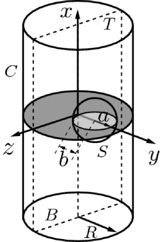
Figure 1: Schematic representation of a spherical squirmer of radius $a$ swimming in a tube of radius $R$. The centre of the squirmer is located at a distance $b$ from the tube axis. The origin of the Cartesian coordinates coincides with the centre of the tube. The bounding surfaces to the fluid are denoted $S$ (surface of squirmer), $B$ (bottom tube cap), $T$ (top tube ca,p) and $C$ (surface of the tube conduit).

The spherical squirmer (radius, $a$) is swimming in a cylindrical tube of radius $R$, as illustrated in figure 1. The centre of the squirmer is located at a distance $b$ from the tube axis. We use Cartesian coordinates with an origin at the centre of the tube and the $x$-direction along the tube axis. As in Higdon & Muldowney (1995) we introduce the nondimensional position $\beta$ as

$$\beta=b/(R-a),$$ (2)

so that $\beta=0$ indicates that the squirmer is at the centre of the tube while for $\beta=1$ the squirmer is in perfect contact with the tube wall.

3 Numerical method

3.1 Formulation

The boundary element method (BEM) has already been successfully adopted to study the hydrodynamics of swimming microorganisms in the Stokesian regime (Ramia et al., 1993; Ishikawa et al., 2006; Shum et al., 2010). Our current work mainly follows the approach in Pozrikidis (2002), the important difference being that we use quadrilateral elements instead of triangle elements as typically used and originally proposed. The method is introduced briefly here.

In the Stokesian realm, fluid motion is governed by the Stokes equation

$$-\nabla p+\mu\nabla^{2}\mathbf{u}=0,$$ (3)

where $p$ is the dynamic pressure and $\mathbf{u}$ the fluid velocity. Due to the linearity of the Stokes equation, the velocity field, $\mathbf{u}\left(\mathbf{x}\right)$, resulting from moving bodies with smooth boundary $S$ can be expressed as

$${}\mathbf{u}\left(\mathbf{x}\right)=\frac{1}{8\pi\mu}\int_{S}\mathbf{f}\left(\mathbf{x}^{\prime}\right)\cdot\mathbf{S}\left(\mathbf{x},\mathbf{x}^{\prime}\right)dS_{\mathbf{x}^{\prime}},$$ (4)

where $\mathbf{f}\left(\mathbf{x}^{\prime}\right)$ is the unknown force per unit area exerted by the body onto the fluid. The tensor $\mathbf{S}$ is the Stokeslet Green’s function

$$\mathbf{S}_{ij}\left(\mathbf{x},\mathbf{x}^{\prime}\right)=\left(\frac{\delta_{ij}}{d}+\frac{d_{i}d_{j}}{d^{3}}\right),$$ (5)

with $d_{i}=x_{i}-x^{\prime}_{i}$, $d^{2}=|\mathbf{x}-\mathbf{x}^{\prime}|^{2}=d_{1}^{2}+d_{2}^{2}+d_{3}^{2}$, and $\delta_{ij}$ denoting the Kronecker delta tensor.

We discretize the two bodies in the problem, namely the spherical squirmer and the surrounding tube, into $N$ zero-order elements with centres at the locations $\{\mathbf{x}_{q},\,q=1\to N\}$, with $q=1\to N_{S}$ denoting the elements on the squirmer surface and $q=N_{S}+1\to N$ the elements on the surface of the tube. For the $r^{th}$ element, $\mathbf{f}\left(\mathbf{x}^{\prime}\right)$ is assumed to be constant over the element and is thus approximated by the value $\mathbf{f}_{r}$. As a consequence, the discretized version of  4 is, when evaluated on one of the elements,

$${}\mathbf{u}\left(\mathbf{x}_{q}\right)=\frac{1}{8\pi\mu}\sum_{r=1}^{N}{\mathbf{f}_{r}}\cdot\int_{S_{r}}\mathbf{S}\left(\mathbf{x}_{q},\mathbf{x}^{\prime}\right)dS_{\mathbf{x}^{\prime}},\,q=1\to N.$$ (6)

In its discrete form, equation 6 represents a total of $3N$ equations for the $3N$ unknown force density components.

3.2 Swimming and squirmer boundary conditions

On the squirmer surface, the left-hand side of 6 is not fully known. The swimmer has an instantaneous surface deformation, $\mathbf{u}_{S}$, plus $6$ unknown components, namely its instantaneous translational velocity vector, $\mathbf{U}$, and its instantaneous rotational velocity vector, $\boldsymbol{\Omega}$. Thus, the left hand side of 6, when evaluated on the surface of the squirmer, becomes $\mathbf{u}\left(\mathbf{x}_{q}\right)=\mathbf{U}+\boldsymbol{\Omega}\times\widetilde{\mathbf{x}}_{q}+\mathbf{u}_{S}\left(\mathbf{x}_{q}\right)$ for $q$ from $1$ to $N_{S}$ (here $\widetilde{\mathbf{x}}_{q}=\mathbf{x}-\mathbf{x}^{R}$, where $\mathbf{x}^{R}$ is an arbitrary reference point, the centre of the spherical squirmer for convenience). The $6$ additional equations necessary to close the linear system are the force- and torque-free swimming conditions, namely

$$\int\mathbf{f}\left(\mathbf{x}\right)dS_{\mathbf{x}}=0,\,\int\widetilde{\mathbf{x}}\times\mathbf{f}\left(\mathbf{x}\right)dS_{\mathbf{x}}=0,$$ (7)

for $\mathbf{x}\in\mathrm{squirmer}$.

3.3 Other boundary conditions

The situation addressed in our paper is that of a squirmer swimming inside an infinitely long tube filled with a quiescent fluid. Numerically, we close both ends of the tube with appropriate boundary conditions. If the tube caps are sufficiently far away from the squirmer, the velocity near the caps is almost zero, so we have $\mathbf{u}_{B}=\mathbf{u}_{T}=\mathbf{0}$, and the pressure over the bottom and top cap is $p_{B}$ and $p_{T}$ respectively (Pozrikidis, 2005). The force density $\mathbf{f}_{T}$ over the top cap can be approximated by $\mathbf{f}_{T}=p_{T}\mathbf{n}$ (Pozrikidis, 2005), where $\mathbf{n}$ is the unit normal vector pointing from the top cap into the fluid domain. Since pressure is defined up to an arbitrary constant, without loss of generality, we set $p_{T}=0$, $\mathbf{f}_{T}=\mathbf{0}$ and the top cap does not requires discretization. However, unlike Pozrikidis (2005), we do perform discretization on the bottom cap, solving for the normal and tangential components of the force density $\mathbf{f}_{B}$ there. For the conduit part of the tube, we use no-slip boundary condition, thus write $\mathbf{u}_{C}=0$.

Since we set the velocity on both caps of the tube to be zero, the error due to domain truncation need to be carefully considered. A truncated tube length $L$ of $\pi R$ or $2\pi R$ was chosen in Pozrikidis (2005) and $L=3R$ in Higdon & Muldowney (1995). In our computation of hydrodynamic force on a moving sphere inside, we tested different values $L$ and examined the truncation error. We find the length, $L=2\pi R$, to be long enough for required accuracy (see figure 3 and details below). In the case of swimming squirmers, we set $L=3\pi R$, and larger values of $L$ were shown to have negligible differences in the results.

3.4 Discretization and integration

Zero-order constant quadrilateral elements are used to discretize all the surfaces. We use six-patch structured grid to discretize the sphere (Higdon & Muldowney, 1995; Cortez et al., 2005; Smith, 2009), mapping six faces of a cube onto the surfaces of a sphere with each face latticed into a square mesh. The conduit part of the tube is divided into cylindrical quadrilateral elements obtained from the intersections of evenly spaced planes normal to tube axis and evenly spaced azimuthal planes (Higdon & Muldowney, 1995; Pozrikidis, 2005; Wen et al., 2007). Moreover, orange-like quadrilateral elements are used for the bottom cap of the tube (Higdon & Muldowney, 1995; Wen et al., 2007). For the sphere we adopt the six-patch quadrilateral grid with parameterized coordinates instead of triangle elements (Pozrikidis, 2002, 2005). Such discretization with its natural parametrisation facilitates Gauss-Legendre quadrature when performing numerical integration. Template points used in the quadrature lie exactly on the sphere surface since their coordinates are derived from the parametrisation. The resulting improved quadrature gives superior accuracy (see Table 1). The integration for singular elements are performed by using plane polar coordinates with Gauss-Legendre quadrature (Pozrikidis, 2002).

In many instances, the squirmer is so close to the cylindrical wall that near-singular integration has to be performed, a key point to achieve the required accuracy and efficiency (Huang & Cruse, 1993). We perform local mesh refinement in the near-contact regions between the squirmer and the tube (Ishikawa et al., 2006; Ishikawa & Hota, 2006) as illustrated in figure 2. The agreement between numerical results with our method and existing results from high-order spectral boundary element method (Higdon & Muldowney, 1995) improves significantly when applying such local mesh refinement as shown in the next section where we compute the resistance of a translating sphere inside a cylindrical tube.

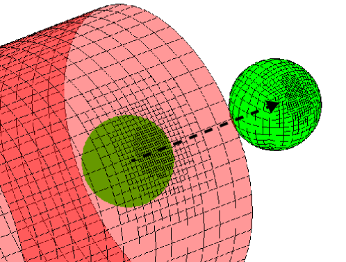
Figure 2: Local mesh refinement of the cylinder (red) and the sphere (green). The geometrical parameters are $a/R=0.3$ and $\beta=0.95$. For a better visualisation, the mesh on the squirmer surface is reproduced on the displaced sphere as indicated by the black arrow.

3.5 Validation and accuracy

We first compute the drag force, $F$, on a translating sphere in an unbounded domain and compare it with the analytical expression, $F=6\pi\mu aU$, where $\mu$ is the dynamic viscosity of the fluid and $U$ is the translational speed of the sphere. As shown in Table 1, the current method is very accurate when compared to the three similar approaches (Pozrikidis, 2002; Cortez et al., 2005; Smith, 2009). We then compute the drag force and torque on a sphere translating parallel to an infinite, flat, no-slip surface. The surface is modelled by a discretized plate of size $40a\times 40a$. Our simulation agree well with analytical results (Goldman et al., 1967), as shown in Table 2. Finally, we compute the drag force acting on a sphere translating inside the tube with confinement $a/R=0.4$, up to a maximum value of $\beta=0.99$, and compare our results with published data obtained with high-order spectral boundary element method (Higdon & Muldowney, 1995). As illustrated in figure 3, the maximum relative error is less than $1.2\%$. In all simulations, the maximum confinement is taken to be $\beta=0.99$ to ensure sufficient accuracy.

	Cortez et al. (2005)	Smith (2009)	Pozrikidis (2002)	This paper
Element Order	0	0	0	0
(functional variation)
Element Type	Quad	Quad	Tri	Quad
Element Number	$6\times 12\times 12$	$6\times 6\times 6$	512	$6\times 6\times 6$
Singular	Regularization	Regularization	Analytical	Analytical
integration	$\epsilon=0.01$	$\epsilon=0.01$	integration	integration
		with adaptive	with	with
		Gauss	Gauss	Gauss
		Quadrature	Quadrature	Quadrature
Relative error ($\%$)	12.6	0.431	9.6 $10^{-3}$	1.4 $10^{-5}$

Table 1: Relative error, in percentage, in the drag force on a translating sphere in an unbounded domain between the method in this paper and three other methods. The parameter $\epsilon$ is the regularization parameter first introduced in Cortez et al. (2005).

$h/a$	$F_{err}\left(\%\right)$	$T_{err}\left(\%\right)$
3.7622	0.00426	0.09488
2.3523	0.01911	0.37879
1.5431	0.04274	0.20478
1.1276	0.07809	0.25773
1.0453	0.09405	0.74217
1.005004	0.17669	1.13493
1.003202	0.27472	1.74313

Table 2: Relative error in the drag force, $F_{err}$, and torque, $T_{err}$, in percentage, on a sphere translating parallel to an infinite wall between our computations and the analytical results (Goldman et al., 1967). Here $a$ is the radius of the sphere and $h$ the distance between the centre of the sphere and the wall.

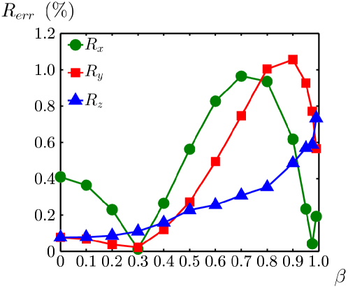
Figure 3: Relative error in the three components of the drag force, $R_{x}$, $R_{y}$, and $R_{z}$, on a sphere translating inside a tube ($a/R=0.4$) between the present paper and Higdon & Muldowney (1995). Note that the three largest values of $\beta$ chosen are $0.95$, $0.975$ and $0.99$.

4 Swimming inside a tube: results

We now have the tools necessary to characterise the locomotion of squirmers inside a tube. Our computational results, presented in this section, are organised as follows. We first compute the swimming kinematics and power consumption of a squirmer instantaneously located at various positions inside the tube while its orientation is kept parallel to the tube axis. These results then enable us to understand the origin of the two-dimensional wave-like trajectory for a neutral squirmer inside the tube. We also analyse the asymptotic stability of trajectories close to solid walls (Yizhar & Richard, 2009; Crowdy & Yizhar, 2010). We then move on to examine the general three-dimensional helical trajectory of a neutral squirmer and also consider the kinematics of pusher and puller swimmers. Finally, we study locomotion induced by normal surface deformation and consider locomotion inside a curved tube.

4.1 Static kinematics and energetics

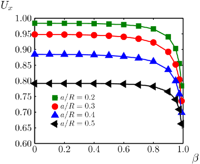
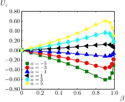
Figure 4: Instantaneous swimming speed for a squirmer in a capillary tube. Left: Swimming velocity in the axial direction, $U_{x}$(independent of $\alpha$), scaled by the swimming speed in free space $U_{ST}^{F}$; different values of $a/R$ are reported with a maximum value of $\beta=0.99$. Right: Swimming velocity $U_{z}$ in the transverse direction, scaled by the swimming speed in free space; here $a/R$ is fixed to $0.3$. Different values of $\alpha$ are reported with maximum value of $\beta=0.99$. In both figures, the squirmer is located at $\left(0,0,-\beta\left(R-a\right)\right)$ with its orientation parallel to the tube axis.

To start our investigation, we first numerically calculate the swimming speed and power consumption for a squirmer exploiting pure tangential surface deformation (for completeness, results on squirmers with normal surface deformations are shown in Sec. 4.6). We fix $B_{1}=1$ and vary the value of $\alpha$, while different values of $a/R$ and $\beta$ are chosen to address the effect of confinement and eccentricity on the instantaneous swimming kinematics.

In figure 4, we plot the instantaneous swimming speed of a squirmer with orientation parallel to the tube axis (positive $\mathbf{x}$ direction) and location $\left(x,y,z\right)=\left(0,0,-\beta\left(R-a\right)\right)$. The swimming velocity parallel to the tube axis ($U_{x}$) is displayed in figure 4 (left) while the velocity perpendicular to it ($U_{z}$) is shown in figure 4 (right). Interestingly, both pushers and pullers have the same swimming speed, $U_{x}$, as the neutral squirmer. This is due to the fact that the second squirming mode, $\sim B_{2}\sin 2\theta$, is front back symmetric, and thus produces zero wall-induced velocity (Berke et al., 2008), as confirmed by our simulation. We observe numerically that when $\alpha=0$, there is only one non-zero velocity component, namely $U_{x}$. In contrast, for pushers and pullers ($\alpha\neq 0$) a non-zero transverse velocity component, $U_{z}$, is induced. The value of $U_{x}$ is seen to decrease with confinement, $a/R$, and eccentricity, $\beta$, as shown in figure 4 (left). The sharp decrease when $\beta$ is beyond $\approx 0.8$ is due to the strong drag force experienced closer to the wall which overcomes the propulsive advantage from near-wall locomotion.

The transverse velocity, $U_{z}$, shown in figure 4 (right), is plotted against the swimmer position, $\beta$, for different values of $\alpha$ while the confinement is fixed at $a/R=0.3$. In the case of a puller ($\alpha>0$), the swimmer will move away from the nearest wall ($U_{z}>0$) while a pusher ($\alpha<0$) will move towards the nearest boundary ($U_{z}<0$), as expected considering the dipolar velocity field generated by squirmers (see also Sec. 4.4). The absolute value of of $U_{z}$ increases with $\alpha$ and is of the same magnitude for pushers and pullers of equal and opposite strength. A similar effect was explained in Berke et al. (2008) for a plane wall, although in that case, the cell was approximated by a point stresslet and the cell-wall distance was considerably larger than the cell size. By probing hydrodynamics very close to the wall, we observe that the magnitude of $U_{z}$ does actually not vary monotonically with $\beta$, instead reaching a maximum value as $\beta\approx 0.9$. Moving away from the tube centre, the transverse velocity increases due to stronger hydrodynamic interactions with the tube walls before decreasing owing to a significantly larger hydrodynamic resistance very close to the tube boundaries.

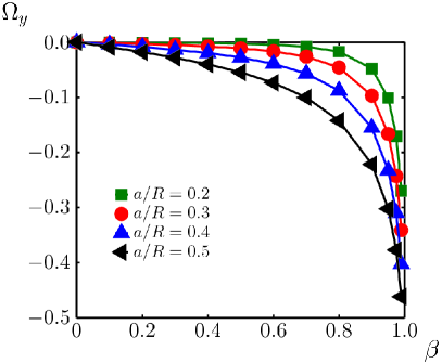
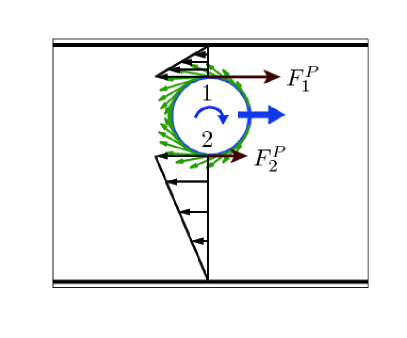
Figure 5: Left: Rotational velocity of the squirmer in the direction normal to the plane of locomotion, $\Omega_{y}$. The squirmer is located at $\left(0,0,-\beta\left(R-a\right)\right)$ with its orientation parallel to the tube axis. Different values of $a/R$ are plotted with maximum value of $\beta=0.99$. Right: Physical picture of cell rotation near the walls. The circle indicates the spherical squirmer and the green arrows denote the tangential surface velocity imposed by the squirmer. Blue straight arrow and curved arrow denote the cell orientation and rotational velocity respectively; $1$ indicates the closest point on the cell to the top wall and $2$ the closest point to the bottom wall while $F^{P}_{1}$ and $F^{P}_{2}$ are the wall-induced shear forces generated near point $1$ and $2$.

Beyond the translational velocities, the squirmers also rotate due to hydrodynamic interactions with the tube boundaries. Numerical results show that the magnitude of the rotational velocity, $\boldsymbol{\Omega}$, is independent on the dipole strength, $\alpha$, and that all squirmers rotate away from the closest wall. This is also attributed to the front-back symmetric distribution of the second squirming mode. Using our notation, we therefore obtain that squirmers rotate in the $-y$ direction. The value of $\Omega_{y}$ is displayed in figure 5 (left). Its magnitude increases with eccentricity, $\beta$, and confinement, $a/R$, as a result of stronger hydrodynamic interactions. To explain the sign of the rotational velocity, we look in detail at a neutral squirmer in figure 5 (right), in the case where the swimmer is located closer to the top wall. Green arrows display the tangential surface deformation which generates locomotion. Given points $1$ and $2$ on the squirmer surface, the black arrows indicate the velocity field and show that the shear rate is higher near point $1$ than point $2$. Consequently, the wall-induced force on point $1$, $F^{P}_{1}$, is larger than that on point $2$, $F^{P}_{2}$, producing a resultant clockwise torque. Since the total torque on the squirmer is zero, the squirmer has to rotate in the clockwise direction to balance this torque, escaping from the top wall. When the squirmer is closer to the top wall, an increased asymmetry will induce a stronger rotation.

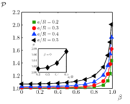
(a) $\quad\alpha=0$

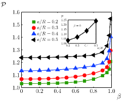
(b) $\quad\alpha=5$

Figure 6: Power consumption, $\mathcal{P}$, of the neutral squirmer ($\alpha=0$, left) and puller ($\alpha=5$, right), scaled by their corresponding values in free space. Insets display $\mathcal{P}$ as a function of $a/R$ in the case $\beta=0$. The orientation of the squirmer is parallel to the tube axis with the maximum value of $\beta=0.99$.

Next, we analyse the power consumption by the squirmer. The power, $\mathcal{P}$, is defined as $\mathcal{P}=\int_{S}\mathbf{f}_{out}\cdot\mathbf{u}_{S}dS$, where $\mathbf{f}_{out}$ is the force per unit area exerted from the outer surface of the body onto the fluid and $\mathbf{u}_{S}$ is the squirming velocity. In the single-layer potential formulation, equation 4 as in Ishikawa et al. (2006), the unknown $\mathbf{f}$ is the sum of the force density from outer ($\mathbf{f}_{out}$) and inner ($\mathbf{f}_{in}$) surface. We therefore rewrite the power as $\mathcal{P}=\int_{S}\mathbf{f}\cdot\mathbf{u}_{S}dS-\int_{S}\mathbf{f}_{in}\cdot\mathbf{u}_{S}dS$, where $\int_{S}\mathbf{f}_{in}\cdot\mathbf{u}_{S}dS$ denotes the viscous dissipation of the flow inside the squirmer. We thus need to subtract the internal viscous dissipation in the fluid given by the numerics where $\mathbf{f}_{in}$ can be derived analytically based on the squirming velocity. In figure 6, we depict the dependence of $\mathcal{P}$, scaled by the corresponding value in free space, with $\beta$ and for different values of $\alpha$. For each gait, $\mathcal{P}$ increases slowly until $\beta\approx 0.8$ followed by a rapid increase for cells closer to the wall. Such a drastic power increase is in agreement with the sharp decrease in swimming speed close to the tube, and consequently, a significant decrease in swimming efficiency is expected. In addition, as the confinement is getting stronger, the eccentricity of the swimmer’s position becomes more important. For example, as $\beta$ changes from $0$ to $0.99$, the power consumption of a neutral squirmer $\mathcal{P}$ increases only by around $45\%$ for $a/R=0.2$ but by $85\%$ for $a/R=0.5$.

4.2 Two-dimensional wavelike motion of the neutral squirmer

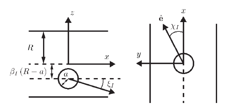
Figure 7: Sketch of the spherical squirmer inside the tube with coordinate system and angles. The initial dimensionless off-axis distance is measured by $\beta_{I}$ while the angles $\xi_{I}$ and $\chi_{I}$ control the initial cell orientation, $\hat{\mathbf{e}}$. For $\chi_{I}=0$, and in the absence of noise, the squirmer motion is restricted to the $x-z$ plane.

We next study in detail the trajectory of a squirmer inside a tube with fixed confinement; unless otherwise stated, all results in this section use the same value, $a/R=0.3$. The cell is neither a pusher nor a puller, but a neutral squirmer generating potential flow field ($\alpha=0$). The initial position and orientation of the cell are defined as in figure 7. The cell is initially placed at $(0,0,-b_{I})$, with $b_{I}=\beta_{I}\left(R-a\right)$, and oriented parallel to the axis ($\xi_{I}=0$); the motion of the cell will also be restricted to the $x-z$ plane ($\chi_{I}=0$). We calculate the translational and rotational velocity of the cell at each time step and update its position using fourth-order Adams-Bashforth scheme as in Giacché & Ishikawa (2010). Note that in the simulations the cell always remains in the centre of the computational domain (while its axial velocity is stored for post-processing), which allows to minimise the error introduced by domain truncation.

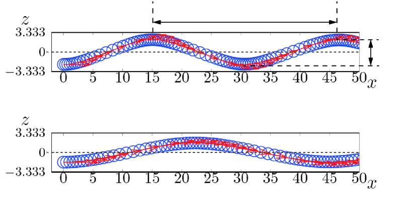
Figure 8: Two-dimensional trajectories of a neutral squirmer inside a capillary tube with confinement $a/R$=0.3. All positions are measured in units of cell radius $a$ (same for figures hereinafter unless otherwise specified). Blue circles and red arrows indicate, respectively, the instantaneous position and orientation of the squirmer. The cell is released from $(0,0,-\beta_{I}\left(R-a\right))$ with $\beta_{I}=0.9$ (up) and $\beta_{I}=0.7$ (bottom), while the initial orientation is parallel to the axis. We denote $\lambda$ the wavelength of the periodic trajectory and $A$ its amplitude.

Our computations show that the squirmer always displays a periodic wavelike trajectory in the tube, with amplitude $A$ and wavelength $\lambda$. This is illustrated in figure 8 for $\beta_{I}=0.9$ (top) and $\beta_{I}=0.7$ (bottom). The wave amplitude does not change over time and is two times the initial off-axis distance, namely, $A=2b_{I}$. The presence of a nonzero rotational velocity, ${\Omega}_{y}$, discussed above and shown in figure 5, is the key parameter leading to the periodic trajectory. By considering cases where the initial orientation of the cell is not parallel to the axis (thus for which the orientation vector has non-zero $x$ and $z$ components) and we find that as long as the squirmer does not immediately descend into the wall, a wavelike trajectory is also obtained. To present all results in a concise manner, we consider the motion of the neutral squirmer as a dynamical system similarly to recent work on two-dimensional swimming (Yizhar & Richard, 2009; Crowdy & Samson, 2011). The trajectory is defined by two parameters, the off-axis distance ($z$) and the angle between the swimmer orientation and the tube axis ($\xi$). We report the phase portrait of the neutral squirmer in the $\left(z,\xi\right)$ plane in figure 9, where the solid curves show the trajectories. The marginally stable point $\left(0,0\right)$ corresponds to locomotion along the axis of the tube. For any initial conditions $\left(z,\xi\right)$, the neutral squirmer swims along wavelike trajectories corresponding to the periodic orbits in figure 9 (the largest periodic orbit in the figure has a maximum $\beta$ of $0.95$).

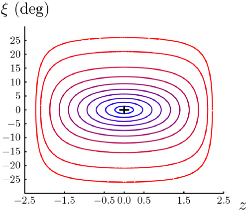
Figure 9: Phase portrait for the neutral squirmer inside the tube in the $\left(z,\xi\right)$ plane with confinement $a/R=0.3$. Closed orbits correspond to $2$D wavelike trajectories. The black cross denotes the equilibrium point $\left(z,\xi\right)=\left(0,0\right)$.

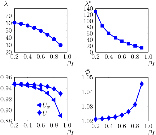
Figure 10: Dynamics and kinematics of the neutral squirmer in a tube as a function of the initial dimensionless off-axis position, $\beta_{I}$. Top left: wavelength, $\lambda$, of the periodic trajectory. Top right: wavelength-to-amplitude ratio, $\lambda^{*}=\lambda/(A/2)$. Bottom left: time-averaged swimming speed in the axial direction, $\bar{U}_{x}$, and along the trajectory, $\bar{U}$, both rescaled by the free-space swimming velocity. Bottom right: time-averaged power consumption $\bar{\mathcal{P}}$, rescaled by value in free space.

The main characteristics of the squirmers’ trajectories are shown in figure 10 for different initial positions, $\beta_{I}$. We display the trajectory wavelength, $\lambda$, and the wavelength-to-amplitude ratio, $\lambda^{\ast}={\lambda}/({A/2})$. It is clear that $\lambda$ and $\lambda^{\ast}$ both decrease with $\beta_{I}$. Indeed, when the swimmer is at the crest or trough of the periodic trajectory, stronger rotation occurs for larger $\beta_{I}$. Therefore, the swimmer will escape from the nearest wall more rapidly, resulting in a decrease of the wavelength. We also show in figure 10 that the time-averaged axial speed, $\bar{U}_{x}$, and the time-averaged swimming speed along the trajectory, $\bar{U}$, decrease with $\beta_{I}$ whereas the time-averaged power consumption, $\bar{\mathcal{P}}$, increases when the squirmers move closer to the wall.

4.3 Three-dimensional helical trajectory of the neutral squirmer

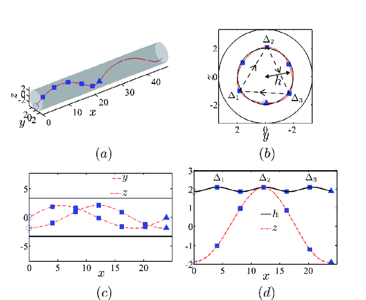
Figure 11: Three-dimensional trajectory of the neutral squirmer in the tube. The initial position and orientation are given by $\beta_{I}=0.8$, $\chi_{I}=30^{\circ}$, $\xi_{I}=0^{\circ}$. (a): trajectory in perspective view; the empty circle and solid triangle indicate the start and end of one periodic orbit; (b): trajectory in the $y-z$ plane (axes shown in figure 11a); (c): trajectories in the $x-y$ (dashed) and $x-z$ (dot dashed) planes; (d): relation between the wavelike motion developed in the axial and azimuthal direction.

By tilting the initial cell orientation, $\hat{\mathbf{e}}$, off the $x-z$ plane, the squirmer trajectories become three dimensional and take the shape of a helix, a feature we address in this section. As in the two-dimensional case, these three-dimensional trajectories are a consequence of hydrodynamics interactions only. Recent experiments in Jana et al. (2012) showed that Paramecium cells display helical trajectories when swimming inside capillary tubes, a feature our simulations are thus able to reproduce. Note that some Paramecium cells also follow helical trajectories in free space due to asymmetries in the shape of their body and the beating of its cilia. In the current work we focus on swimmers whose helical dynamics arises only in confinement.

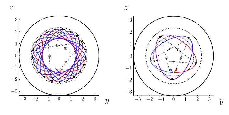
Figure 12: Periodic orbits of the neutral squirmer in the transverse plane for two different initial positions and orientations. Left: $\left(\beta_{I},\chi_{I}\right)=\left(0.6,30^{\circ}\right)$. Right: $\left(\beta_{I},\chi_{I}\right)=\left(0.6,20^{\circ}\right)$.

We introduce $\chi_{I}$ as the yaw angle between the initial cell orientation and the $x-z$ plane (see figure 7), so that the initial orientation becomes $\left(\cos\left(\chi_{I}\right),\sin\left(\chi_{I}\right),0\right)$. In our simulations, $\beta_{I}$ ranges from $0.3$ to $0.9$ and $\chi_{I}$ from $20^{\circ}$ to $40^{\circ}$. Within these parameters, squirmers always display helical trajectories. One such helix is plotted in figure 11, for an initial position $\beta_{I}=0.8$ and a yaw angle $\chi_{I}=40^{\circ}$. The helical trajectory is a combination of wavelike motions developed in the azimuthal $y-z$ plane and in the axial direction, see figure 11b and c. In figure 11b, we show the projected circular trajectory of the swimmer in the $y-z$ plane. In figure 11c, we show that the curves $y\left(x\right)$ and $z\left(x\right)$ share the same wavelength and time period. We then plot the values of $z$ and $h$ (cell off-axis distance) as a function of the axial position, $x$, during one period in figure 11d to show that the wave frequency of $h\left(x\right)$ is three times that of $z\left(x\right)$. Indeed, the trajectory projected in the plane perpendicular to the tube axis resembles a regular triangle ($\Delta_{1}\Delta_{2}\Delta_{3}$), with vertices corresponding to locations of maximum off-axis distance where the cell bounces back inside the tube. In this particular case, the cell bounces off the wall three times during one orbit with an angle $\psi=60^{\circ}$. A variety of other wave patterns can be observed for different initial cell positions and yaw angels $\left(\beta_{I},\chi_{I}\right)$. We display two of them in figure 12 in the $y-z$ plane, with $\left(\beta_{I},\chi_{I}\right)=\left(60,30^{\circ}\right)$ (figure 12, left) and $\left(60,20^{\circ}\right)$ (figure 12, right). The swimmer on the left approaches the wall $21$ times during one periodic orbit with $\psi=42.86^{\circ}$, whereas the example on the right displays a $5$ fold helix with $\psi=36^{\circ}$.

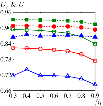
Figure 13: Nondimensional time-averaged swimming speed and power consumption of squirmers with different initial position ($\beta_{I}$) and orientation ($\chi_{I}$) with three-dimensional kinematics.

Finally in figure 13 we show the variation of the averaged swimming speed (left) and power consumption (right) with the initial cell position ($\beta_{I}$) and orientation ($\chi_{I}$), where both the speed and power are nondimensionalized by their corresponding values in free space. The time-averaged swimming speed along the axial direction, $\bar{U}_{x}$, and along the trajectory, $\bar{U}$, decrease clearly with $\chi_{I}$ but slowly with $\beta_{I}$. Larger values of $\chi_{I}$ and $\beta_{I}$ result in larger maximum off-axis distance, leading to higher hydrodynamic resistance from the boundaries and thus hindering locomotion. We also observe that $\bar{U}_{x}$ decreases with $\chi_{I}$ more rapidly than $\bar{U}$. As $\chi_{I}$ increases, the swimmer trajectory becomes more coiled, which significantly decreases the swimming velocity in the axial direction. We also note that the power consumption, $\bar{\mathcal{P}}$, increases with the the initial orientation, $\chi_{I}$, but does not change significantly with $\beta_{I}$.

4.4 The trajectory of a puller inside the tube

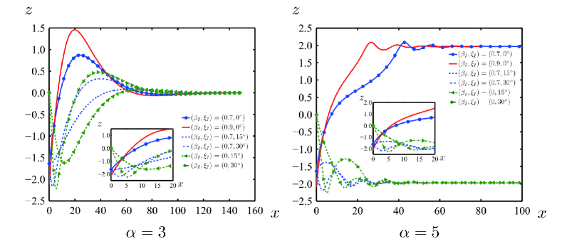
Figure 14: Two-dimensional trajectories, $z(x)$, of pullers in a tube (left: $\alpha=3$; right: $\alpha=5$). Different combinations of the initial position ($\beta_{I}$) and pitching angle ($\xi_{I}$) are chosen. The inset plots display the trajectories near the starting positions.

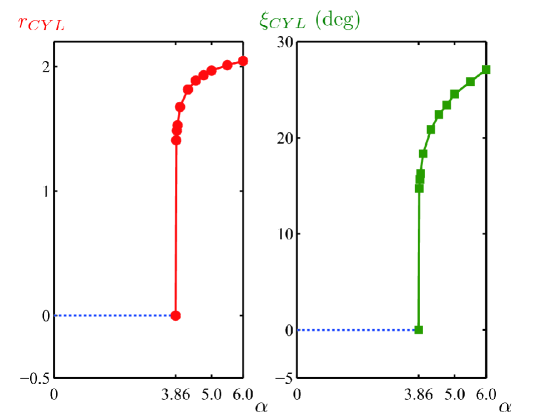
Figure 15: Equilibrium points, $\left\{r_{CYL},\xi_{CYL}\right\}$, of the puller in the tube as a function of the the dipole strength, $\alpha$, and for a confinement $a/R=0.3$. Blue dashed lines ($\alpha<3.86$) show the equilibrium point at $\left(0,0\right)$, corresponding to swimming in the centre of the tube and along its axis. For $\alpha>3.86$, the combination $\left\{r_{CYL},\xi_{CYL}\right\}$ characterises the equilibrium state for swimming along a straight line with off-axis distance $r_{CYL}$ and orientation towards the wall $\xi_{CYL}$.

In this section, we study the trajectories of a puller swimmer ($\alpha>0$) in the tube. We first consider the case where the motion is restricted to the $x-z$ plane, as in Sec. 4.2. In figure 14 we show the two-dimensional trajectories of pullers having dipole parameters of $\alpha=3$ (left) and $\alpha=5$ (right), for different initial positions, $\beta_{I}$, and orientations, $\xi_{I}$. In both cases, the swimmers initially follow wavelike trajectories with decreasing magnitude, and eventually settle along straight trajectories, displaying thus passive asymptotic stability (Yizhar & Richard, 2009). The puller with $\alpha=3$ ends up swimming along the tube axis, with $\left(r_{CYL},\xi_{CYL}\right)=\left(0,0\right)$ as its equilibrium point (cylindrical coordinates are used here, and $r_{CYL}$ and $\xi_{CYL}$ denote the off-axis distance and orientation of the cell respectively). In contrast, the puller with $\alpha=5$ swims parallel to the axis near the top or bottom wall depending on its initial position and orientation, thus its equilibrium point corresponds to swimming along an off-axis straight line. In that case, even though the trajectory is parallel to the tube axis, the swimmer remains slightly inclined towards the wall to offset the hydrodynamic repulsion from the wall.

We further examine the coordinates of equilibrium points $\left(r_{CYL},\xi_{CYL}\right)$ as a function of the dipole strength, $\alpha$, in figure 15. For $\alpha$ below a critical value, $\alpha_{c}\approx 3.86$ for the confinement chosen here ($a/R=0.3$), the equilibrium point is $\left(r_{CYL},\xi_{CYL}\right)=\left(0,0\right)$ denoted by the dashed blue line. For $\alpha>3.86$, the equilibrium point corresponds to swimming stably along a straight line with off-axis distance $r_{CYL}$ and orientation $\xi_{CYL}$, both of which grow with increasing $\alpha$. The relationship between confinement, $a/R$, and the critical value $\alpha_{c}$ is examined in figure 16. Determining precisely the value of $\alpha_{c}$ is not possible due to the large computational cost so we report approximate values, with an upper (resp. lower) limit of the error bar corresponding to the asymptotically-stable swimming motion near the wall (resp. along the tube axis). The critical dipolar strength first increases with the confinement, reaching its maximum as $a/R\approx 0.3$, before decreasing.

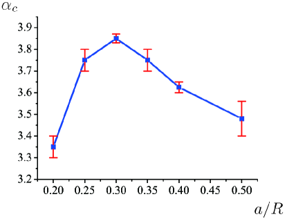
Figure 16: Critical value of the dipole parameter, $\alpha_{c}$, for stable swimming of the puller in the tube centre as a function of the confinement, $a/R$. The approximate values of $\alpha_{c}$ are denoted by the square symbols and the upper (resp. lower) limit of the error bar corresponds to the asymptotically-stable swimming motion away from the centre (resp. along the tube axis).

By starting with different combinations of $\alpha$, $\beta_{I}$ and $\chi_{I}$, we obtain different three-dimensional trajectories for the puller. Some of these trajectories are illustrated in figure 17. Results similar to the two-dimensional simulations are obtained. For $\alpha$ below a critical value, pullers eventually swim along the tube axis indicating the equilibrium point $\left(r_{CYL},\xi_{CYL}\right)=\left(0,0\right)$. For larger values of $\alpha$, the equilibrium point corresponds to swimming motion with constant off-axis distance and orientation. Hydrodynamic interactions between the swimmer and the tube alone are responsible for such a passive stability, which could be of importance to guarantee, for example, robust steering of artificial micro-swimmers in capillary tubes without on-board sensing and control (Yizhar & Richard, 2009).

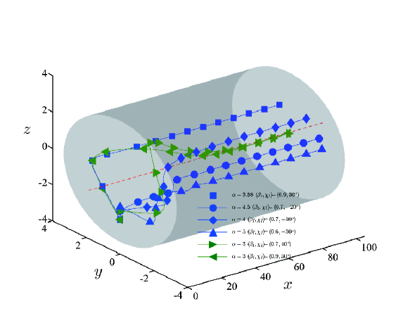
Figure 17: Three-dimensional trajectories of pullers in the tube with confinement $a/R=0.3$. The red dashed line indicates the tube axis. Different combinations of the dipole strength, $\alpha$, initial position, $\beta_{I}$, and initial orientation, $\chi_{I}$, are chosen. Green trajectories correspond to pullers with one equilibrium point in the tube centre whereas blue ones are for pullers with equilibrium near the wall.

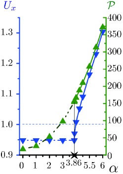
Figure 18: Swimming speed, $U_{x}$ (blue lower triangles), and power consumption, $\mathcal{P}$ (green upper triangles), of the puller as a function of the dipole parameter, $\alpha$, both quantities being scaled by their corresponding values in free space (with $a/R=0.3$). The critical value $\alpha_{c}=3.86$, shown by the cross, is the transition between stable swimming at the tube centre vs. stable swimming near the tube walls. The blue dashed line indicates the swimming speed in free space.

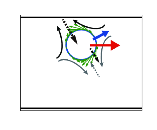
Figure 19: The orientation, $\hat{\mathbf{e}}$, of a puller swimming (red arrow) on the stable trajectory near the tube wall. Curved green arrows stand for the flow imposed at the surface of the swimmer, black ($\mathbf{F}_{N}^{P}$) and grey ($\mathbf{F}_{F}^{P}$) dashed arrows for the hydrodynamic force while $\mathbf{F}_{R}$ is the repulsive force.

We conclude this section by investigating in figure 18 the swimming speed of the puller along the stable trajectory and the dependency of its magnitude on the dipole strength, $\alpha$. In the case of confinement $a/R=0.3$, the swimming speed $U_{x}$ is larger than that in free space as $\alpha$ is above a critical value (around $4$ here) and it increases by about $16\%$ as $\alpha=5$. This is an example of swimming microorganisms taking propulsive advantage from near-wall hydrodynamics, as discussed in previous analytical studies (Katz, 1974; Felderhof, 2009, 2010). In our case, as the squirmer is oriented into the wall, the direction of the wall-induced hydrodynamic force, $F_{R}$, resulting from flow being ejected on the side of the puller, is not normal to the wall but possesses a component in the swimming direction, as shown in figure 19. This force contributes thus to an additional propulsion and increases the swimming speed.

4.5 The trajectory of a pusher inside the tube

We next address the spherical pusher squirmer, with a negative force dipole, $\alpha$. We find that the motion of the pushers inside the tube is unstable. The trajectories of pushers confined in the $x-z$ plane ($\chi_{I}=0$) are plotted in figure 20 for different combinations of dipole strength, initial position, and initial orientation. The pushers always execute wavelike motions with decreasing wavelengths and increasing amplitude, eventually crashing into the walls. Pushers and pullers display therefore very different swimming behaviours, a difference which stems from the opposite front-back asymmetry of the force dipole.

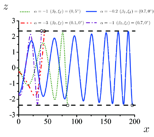
Figure 20: Two-dimensional trajectories of pushers for different combinations of $\alpha$, $\beta_{I}$, and $\xi_{I}$. The black circles indicate the moment the swimmers make contact with the wall.

4.6 Squirmers with normal surface velocity

For the sake of completeness, we investigate in this section the dynamics of squirmers in the tube in the case where the squirming motion is induced by normal (instead of tangential) surface velocity, modelled as

$$\mathbf{u}_{SN}({\bf r})=\sum_{n=0}\frac{2}{n(n+1)}A_{n}P_{n}\left(\frac{\hat{\bf{e}}\cdot\mathbf{r}}{r}\right),$$ (8)

where $A_{n}$ is the $n$th mode of the normal squirming velocity (Blake, 1971). In free space, the swimming velocity is $U_{SN}^{F}=-{A_{1}}/{3}$ (Blake, 1971). For simplicity, we only consider the instantaneous kinematics of a squirmer with $A_{1}=-1$ and $A_{n\neq 1}=0$, corresponding thus to $U_{SN}^{F}={1}/{3}$. The swimmer is located at $\left(0,0,-\beta\left(R-a\right)\right)$, and is oriented in the positive $\mathbf{x}$ direction. We plot the axial velocity component, $U_{x}$, (scaled by $U_{SN}^{F}$) together with the rotational velocity, $\Omega_{y}$, in figure 21. Both $U_{x}$ and $\Omega_{y}$ are seen to increase monotonically with the confinement and eccentricity. This is in agreement with past mathematical analysis stating that microorganisms utilising transverse surface displacement speed up when swimming near walls (Katz, 1974), between two walls (Felderhof, 2009), or inside a tube (Felderhof, 2010).

This increase (resp. decrease) of swimming speed in the tube of a squirmer with normal (resp. tangential) surface deformation can be related to the problem of micro-scale locomotion in polymeric solutions. It is well known that actuated biological flagella generate drag-based thrust due to larger resistance to normal than to tangential motion (Lauga & Powers, 2009). When swimming in polymer solutions, flagella undergoing motion normal to its shape push directly onto the neighbouring polymer network, whereas tangential motion barely perturb these micro obstacles (Berg & Turner, 1979; Magariyama & Kudo, 2002; Nakamura et al., 2006; Leshansky, 2009). In this case, the drag force increases more in the normal direction than in the tangential, resulting in larger swimming speeds (Berg & Turner, 1979; Magariyama & Kudo, 2002; Nakamura et al., 2006; Leshansky, 2009; Liu et al., 2011). Likewise, it was shown for a spherical squirmer that polymeric structures in the fluid always decrease the swimming speed in case of tangential surface deformation (Leshansky, 2009; Zhu et al., 2011, 2012) but increase for normal deformation (Leshansky, 2009). The increase of swimming speed observed here in the case of a squirmer with normal surface deformation can similarly be attributed to the flow directly onto the tube wall.

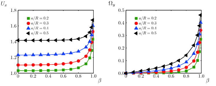
Figure 21: Swimming velocity in the axial direction, $U_{x}$, and rotational velocity, $\Omega_{y}$, of the squirmer with normal surface deformation with modes $A_{n}=-\delta_{n1}$; $U_{x}$ is scaled by the swimming speed in free space, $U_{SN}^{F}$. The squirmer is located at $\left(0,0,-\beta\left(R-a\right)\right)$ and oriented parallel to the axis. Different values of $a/R$ are reported with maximum value of $\beta=0.99$.

The value of rotational velocity, $\Omega_{y}$, shown in figure 21 shows however that the squirmer rotates into the nearest wall, thus getting eventually trapped there. In order to avoid being trapped while at the same time taking advantage of the wall-induced enhanced propulsion, ideally swimmers should thus use a combination of tangential and normal deformation.

Interestingly, a superposition of the neutral squirming mode ($B_{n}=\delta_{n1}$, see §2) with the first normal squirming mode ($A_{n}=-\delta_{n1}$) results in a special swimmer able to move without creating any disturbance in the surrounding fluid, characterised by a uniform squirming velocity of $-1$ everywhere on the body (in the co-moving frame), no body rotation, and a swimming speed equal to $1$. This remains true regardless of the degree of confinement as confirmed by our numerical simulations.

5 Swimming inside a curved tube

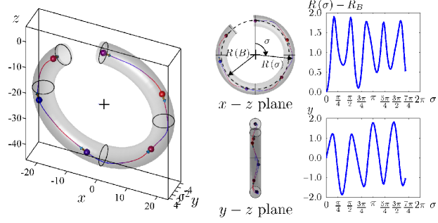
Figure 22: Three-dimensional swimming of the neutral squirmer inside a torus-like curved tube. The dashed line indicates the circular axis of the torus with its radius, $R_{B}=20a$, $\sigma$ is the azimuthal position of the squirmer, and $R\left(\sigma\right)$ is the distance between the squirmer and the centre of the baseline circle. The wavelike motions for $R\left(\sigma\right)-R_{B}$ and $y(\sigma)$ are shown on the right.

In this final section, we investigate the squirmer motion inside a curved tube that is a part of a torus. The axis of the torus is a circle on the plane $y=0$ with its radius $R_{B}=20a$. Trajectories of a neutral squirmer and a puller with the dipole strength $\alpha=1$ are shown in Figs. 22 and 23 respectively. In both cases, the trajectory is displayed in both the $x-z$ and $y-z$ planes. The motion in the radial direction, represented by $R\left(\sigma\right)-R_{B}$, is plotted as a function of the azimuthal position of the swimmer, $\sigma$, where $R\left(\sigma\right)$ is the distance between the cell and the centre of the circle. In both cases, the dynamics of swimmers initially starting aligned with the tube axis is wavelike. For the neutral squirmer, the wavelength and wave magnitude approach a constant value $\sigma>\pi$ (figure 22, right), indicating marginal stability of the motion. In contrast, for the puller, decaying waves are observed (figure 23, right), indicating passive asymptotic stability. As in the straight-tube case, pushers are unstable and crash into walls in finite time.

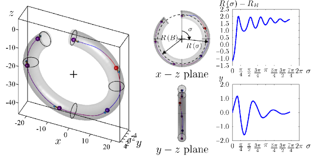
Figure 23: Same as in figure 22 but for a puller with $\alpha=1$.

6 Conclusion and outlook

In this paper, a Boundary Element Method code was developed, validated, and used to present computations for the locomotion of model ciliates inside straight and curved capillary tubes. We used the spherical squirmer as our model microorganism and studied the effect of confinement on the kinematics, energetics, and trajectories of the cell. We also investigated the stability of the swimming motion of squirmers with different gaits (neutral, pusher, puller).

We found that tube confinement and near-wall swimming always decrease the swimming speed of a squirmer with tangential surface deformation for swimming parallel to the tube axis. In contrast, a swimmer with normal surface deformation improves its swimming speed by directly pushing against the surrounding tube wall. In both cases however, tube confinement and near-wall swimming always lead to additional viscous dissipation, thus increasing the power consumption.

Focusing on swimming with tangential forcing, we then studied in detail the dynamics of neutral, puller, and pusher squirmers inside a straight tube. For a neutral squirmer, swimming motion on the tube axis is marginally stable and generically displays three-dimensional helical trajectories as previously observed experimentally for Paramecium cells. Importantly, these helical trajectories arise purely from hydrodynamic interactions with the boundaries of the tube.

In the case of puller swimmers, their trajectories are wavelike with decreasing amplitude and increasing wavelength, eventually leading to stable swimming parallel with the tube axis with their bodies slightly oriented toward the nearest wall. The locations for these stable trajectories depend on the strength of the force dipole, $\alpha$. Swimmers with weak dipoles (small $\alpha$) swim in the centre of the tube while those with strong dipoles (large $\alpha$) swim near the walls. The stable orientation of the swimmers makes an non-zero contribution of the wall-induced hydrodynamic forces in the direction of locomotion, thus leading to an increase of the swimming speed (although accompanied by an increase of the rate of viscous dissipation). In contrast, pushers are always unstable and crash into the walls of the tube in finite time. Similar results are observed for locomotion inside a curved tube.

We envision that our study and general methodology could be useful in two specific cases. First, our results could help shed light on and guide the future design and maneuverability of artificial small-scale swimmers inside small tubes and conduits. Second, the computational method could be extended to more complex, and biologically-relevant, geometries, to study for example the locomotion of flagellated bacteria or algae into confined geometries, as well as their hydrodynamic interactions with relevant background flows. It would be also interesting to relax some of our assumptions in future work, and address the role of swimmer geometry on their stability (we only considered the case of spherical swimmers in our paper) and quantify the role of noise and fluctuations on the asymptotic dynamics obtained here.

References

- Berg (2000) Berg, H. C. 2000 Motile behavior of bacteria. Phys. Today 53, 24–29.
- Berg & Turner (1979) Berg, H. C. & Turner, L. 1979 Movement of microorganisms in viscous environments. Nature 278, 349–351.
- Berke et al. (2008) Berke, A. P., Turner, L., Berg, H. C. & Lauga, E. 2008 Hydrodynamic attraction of swimming microorganisms by surfaces. Phys. Rev. Lett. 101, 038102.
- Biondi et al. (1998) Biondi, S. A., Quinn, J. A. & Goldfine, H. 1998 Random mobility of swimming bacteria in restricted geometries. AIChE J. 44, 1923–1929.
- Blake (1971) Blake, J. R. 1971 A spherical envelope approach to ciliary propulsion. J. Fluid Mech. 46, 199–208.
- Brennen & Winet (1977) Brennen, C. & Winet, H. 1977 Fluid mechanics of propulsion by cilia and flagella. Annu. Rev. Fluid Mech. 9, 339–398.
- Cortez et al. (2005) Cortez, R., Fauci, L. & Medovikov, A. 2005 The method of regularized stokeslets in three dimensions: Analysis, validation, and application to helical swimming. Phys. Fluids 17, 031504.
- Crowdy & Samson (2011) Crowdy, D. & Samson, O. 2011 Hydrodynamic bound states of a low-reynolds-number swimmer near a gap in a wall. J. Fluid Mech. 667, 309–335.
- Crowdy & Yizhar (2010) Crowdy, D. & Yizhar, O. 2010 Two-dimensional point singularity model of a low-reynolds-number swimmer near a wall. Phys. Rev. E 81, 036313.
- Dombrowski et al. (2004) Dombrowski, C., Cisneros, L., Chatkaew, S., Goldstein, R. E. & Kessler, J. O. 2004 Self-concentration and large-scale coherence in bacterial dynamics. Phys. Rev. Lett. 93, 098103.
- Doostmohammadi et al. (2012) Doostmohammadi, A., Stocker, R. & Ardekani, A. M. 2012 Low-reynolds-number swimming at pycnoclines. Proc. Natl. Acad. Sci. USA 109, 3856–3861.
- Drescher et al. (2011) Drescher, K., Dunkel, J., Cisneros, L. H., Ganguly, S. & Goldstein, R. E. 2011 Fluid dynamics and noise in bacterial cell-cell and cell-surface scattering. Proc. Natl. Acad. Sci. USA 108, 10940–10945.
- Drescher et al. (2010) Drescher, K., Goldstein, R. E., Michel, N., Polin, M. & Tuval, I. 2010 Direct measurement of the flow field around swimming microorganisms. Phys. Rev. Lett. 105, 168101.
- Drescher et al. (2009) Drescher, K., Leptos, K. C., Tuval, I., Ishikawa, T., Pedley, T. J. & Goldstein, R. E. 2009 Dancing Volvox : Hydrodynamic bound states of swimming algae. Phys. Rev. Lett. 102, 168101.
- Durham et al. (2009) Durham, W. M., Kessler, J. O. & Stocker, R. 2009 Disruption of vertical motility by shear triggers formation of thin phytoplankton layers. Science 323, 1067–1070.
- Elfring et al. (2010) Elfring, G., Pak, O. S. & Lauga, E. 2010 Two-dimensional flagellar synchronization in viscoelastic fluids. J. Fluid Mech. 646, 505–515.
- Evans et al. (2011) Evans, A. A., Ishikawa, T., Yamaguchi, T. & Lauga, E. 2011 Orientational order in concentrated suspensions of spherical microswimmers. Phys. Fluids 23, 111702.
- Fauci & Dillon (2006) Fauci, L. J. & Dillon, R. 2006 Biofluidmechanics of reproduction. Annu. Rev. Fluid Mech. 38, 371–394.
- Fauci & Mcdonald (1995) Fauci, L. J. & Mcdonald, A. 1995 Sperm mobility in the presence of boundaries. Bull. Math. Biol. 57, 679–699.
- Felderhof (2009) Felderhof, B. U. 2009 Swimming and peristaltic pumping between two plane parallel walls. J. Phys. Condens. Matter 21, 204106.
- Felderhof (2010) Felderhof, B. U. 2010 Swimming at low reynolds number of a cylindrical body in a circular tube. Phys. Fluids 22, 113604.
- Fu et al. (2008) Fu, H., Powers, T. R. & Wolgemuth, C. W. 2008 Theory of swimming filaments in viscoelastic media. Phys. Rev. Lett. 99, 258101.
- Giacché & Ishikawa (2010) Giacché, D. & Ishikawa, T. 2010 Hydrodynamic interaction of two unsteady model microorganisms. J. Theor. Biol 267, 252–263.
- Goldman et al. (1967) Goldman, A.J., Cox, R.G. & Brenner, H. 1967 Slow viscous motion of a sphere parallel to a plane wall—i motion through a quiescent fluid. Chem. Eng. Sci 22, 637 – 651.
- Goto et al. (2005) Goto, T., Nakata, K., Baba, K., Nishimura, M. & Magariyama, Y. 2005 A fluid-dynamic interpretation of the asymmetric motion of singly flagellated bacteria swimming close to a boundary. Biophys. J. 89, 3771–3779.
- Guasto et al. (2010) Guasto, J. S., Johnson, K. A. & Gollub, J. P. 2010 Oscillatory flows induced by microorganisms swimming in two dimensions. Phys. Rev. Lett. 105, 168102.
- Hamel et al. (2011) Hamel, A., Fisch, C., Combettes, L., Dupuis-Williams, P. & Baroud, C. N. 2011 Transitions between three swimming gaits in paramecium escape. Proc. Natl. Acad. Sci. USA 108, 7290–7295.
- Higdon & Muldowney (1995) Higdon, J. J. L. & Muldowney, G. P. 1995 Resistance functions for spherical particles, droplets and bubbles in cylindircal tubes. J. Fluid Mech. 298, 193–210.
- Hill et al. (2007) Hill, J., Kalkanci, O., McMurry, J. L. & Koser, H. 2007 Hydrodynamic surface interactions enable Escherichia Coli to seek efficient routes to swim upstream. Phys. Rev. Lett. 98, 068101.
- Huang & Cruse (1993) Huang, Q. & Cruse, T. A. 1993 Some notes on singular integral techniques in boundary element analysis. Int. J. Numer. Meth. Eng 36, 2643–2659.
- Ishikawa (2009) Ishikawa, T. 2009 Suspension biomechanics of swimming microbes. J. R. Soc. Interface 6, 815–834.
- Ishikawa & Hota (2006) Ishikawa, T. & Hota, M. 2006 Interaction of two swimming paramecia. J. Exp. Biol. 209, 4452–4463.
- Ishikawa & Pedley (2008) Ishikawa, T. & Pedley, T. J. 2008 Coherent structures in monolayers of swimming particles. Phys. Rev. Lett. 100, 088103.
- Ishikawa et al. (2006) Ishikawa, T., Simmonds, M. P. & Pedley, T. J. 2006 Hydrodynamic interaction of two swimming model micro-organisms. J. Fluid Mech. 568, 119–160.
- Jana et al. (2012) Jana, S., Um, S. H. & Jung, S. 2012 Paramecium swimming in capillary tube. Phys. Fluids 24, 041901.
- Katz (1974) Katz, D. F. 1974 On the propulsion of micro-organisms near solid boundaries. J. Fluid Mech. 64, 33–49.
- Katz (1975) Katz, D. F. 1975 On the movement of slender bodies near plane boundaries at low reynolds number. J. Fluid Mech. 72, 529–540.
- Kaya & Koser (2012) Kaya, T. & Koser, H. 2012 Direct upstream motility in Escherichia coli. Biophys. J. 102, 1514–1523.
- Lauga (2007) Lauga, E. 2007 Propulsion in a viscoelastic fluid. Phys. Fluids 19, 083104.
- Lauga et al. (2006) Lauga, E., DiLuzio, W. R., Whitesides, G. M. & Stone, H. A. 2006 Swimming in circles: Motion of bacteria near solid boundaries. Biophys. J. 90, 400–412.
- Lauga & Powers (2009) Lauga, E. & Powers, T. R. 2009 The hydrodynamics of swimming microorganisms. Rep. Prog. Phys. 72, 096601.
- Leonardo et al. (2011) Leonardo, R. Di, Dell’Arciprete, R., Angelani, L. & Iebba, V. 2011 Swimming with an image. Phys. Rev. Lett. 106, 038101.
- Leshansky (2009) Leshansky, A. M. 2009 Enhanced low-Reynolds-number propulsion in heterogeneous viscous environments. Phys. Rev. E 80, 051911.
- Lighthill (1975) Lighthill, J. 1975 Mathematical Biofluiddynamics. Philadelphia, PA: SIAM.
- Lighthill (1976) Lighthill, J. 1976 Flagellar hydrodynamics - The John von Neumann lecture, 1975. SIAM Rev. 18, 161–230.
- Lighthill (1952) Lighthill, M. J. 1952 On the squirming motion of nearly spherical deformable bodies through liquids at very small Reynolds numbers. Comm. Pure Appl. Math. 5, 109–118.
- Lin et al. (2011) Lin, Z., Thiffeault, J. & Childress, S. 2011 Stirring by squirmers. J. Fluid Mech. 669, 167–177.
- Liu et al. (2011) Liu, B., Powers, T. R. & Breuer, K. S. 2011 Force-free swimming of a model helical flagellum in viscoelastic fluids. Proc. Natl. Acad. Sci. USA 108, 19516–19520.
- Magar et al. (2003) Magar, V., Goto, T. & Pedley, T. J. 2003 Nutrient uptake by a self-propelled steady squirmer. Q. J. Mech. Appl. Math. 56, 65–91.
- Magariyama & Kudo (2002) Magariyama, Y. & Kudo, S. 2002 A mathematical explanation of an increase in bacterial swimming speed with viscosity in linear-polymer solutions. Biophys. J. 83, 733–739.
- Nakamura et al. (2006) Nakamura, S., Adachi, Y., Goto, T. & Magariyama, Y. 2006 Improvement in motion efficiency of the spirochete Brachyspira pilosicoli in viscous environments. Biophys. J. 90, 3019–3026.
- Nguyen et al. (2011) Nguyen, H., Ortiz, R., Cortez, R. & Fauci, L. 2011 The action of waving cylindrical rings in a viscous fluid. J. Fluid Mech. 671, 574–586.
- Polin et al. (2009) Polin, M., Tuval, I., Drescher, K., Gollub, J. P. & Goldstein, R. E. 2009 Chlamydomonas swims with two gears in a eukaryotic version of run-and-tumble locomotion. Science 24, 487–490.
- Pozrikidis (2002) Pozrikidis, C. 2002 A practical guide to boundary element methods with the software library BEMLIB, 1st edn. CRC Press.
- Pozrikidis (2005) Pozrikidis, C. 2005 Computation of stokes flow due to motion or presence of a particle in a tube. J. Eng. Math 53, 1–20.
- Purcell (1977) Purcell, E. M. 1977 Life at low Reynolds number. Am. J. Phys. 45, 3–11.
- Ramia et al. (1993) Ramia, M., Tullock, D. L. & Phan-Thien, N. 1993 The role of hydrodynamic interaction in the locomotion of microorganisms. Biophys. J. 65, 755–778.
- Shen & Arratia (2011) Shen, X. N. & Arratia, P. E. 2011 Undulatory swimming in viscoelastic fluids. Phys. Rev. Lett. 106, 208101.
- Shum et al. (2010) Shum, H., Gaffney, E. A. & Smith, D. J. 2010 Modelling bacterial behaviour close to a no-slip plane boundary: the influence of bacterial geometry. Proc. R. Soc. A 466, 1725–1748.
- Smith (2009) Smith, D. J. 2009 A boundary element regularized stokeslet method applied to cilia- and flagella-driven flow. Proc. R. Soc. A 465, 3605–3626.
- Smith et al. (2009) Smith, D. J., Gaffney, E. A., Blake, J. R. & Kirkman-Brown, J. C. 2009 Human sperm accumulation near surfaces: a simulation study. J. Fluid Mech. 621, 289–320.
- Spagnolie & Lauga (2012) Spagnolie, S. E. & Lauga, E. 2012 Hydrodynamics of self-propulsion near a boundary: predictions and accuracy of far-field approximations. J. Fluid Mech. 700, 105–147.
- Stocker & Durham (2009) Stocker, R. & Durham, W. M. 2009 Tumbling for stealth? Science 24, 400–402.
- Underhill et al. (2008) Underhill, P. T., Hernandez-Ortiz, J. P. & Graham, M. D. 2008 Diffusion and spatial correlations in suspensions of swimming particles. Phys. Rev. Lett. 100, 248101.
- Wen et al. (2007) Wen, P. H., Aliabadi, M. H. & Wang, W. 2007 Movement of a spherical cell in capillaries using a boundary element method. J. Biomech 40, 1786–1793.
- Winet (1973) Winet, H. 1973 Wall drag on free-moving ciliated micro-organisms. J. Exp. Biol 59, 753–766.
- Yates (1986) Yates, G. T. 1986 How microorganisms move through water: The hydrodynamics of ciliary and flagellar propulsion reveal how microorganisms overcome the extreme effect of the viscosity of water. Am. Sci 74, 358–365.
- Yizhar & Richard (2009) Yizhar, O. & Richard, M. M. 2009 Dynamics and stability of a class of low reynolds number swimmers near a wall. Phys. Rev. E 79, 045302.
- Zhu et al. (2011) Zhu, L., Do-Quang, M., Lauga, E. & Brandt, L. 2011 Locomotion by tangential deformation in a polymeric fluid. Phys. Rev. E 83, 011901.
- Zhu et al. (2012) Zhu, L., Lauga, E. & Brandt, L. 2012 Self-propulsion in viscoelastic fluids: pushers vs. pullers. Phys. Fluids 24, 051902.
- Zöttl & Stark (2012) Zöttl, A. & Stark, H. 2012 Nonlinear dynamics of a microswimmer in poiseuille flow. Phys. Rev. Lett. 108, 218104.