Chip-level and multi-node analysis of energy-optimized lattice-Boltzmann CFD simulations

Abstract

Memory-bound algorithms show complex performance and energy consumption behavior on multicore processors. We choose the lattice-Boltzmann method (LBM) on an Intel Sandy Bridge cluster as a prototype scenario to investigate if and how single-chip performance and power characteristics can be generalized to the highly parallel case. First we perform an analysis of a sparse-lattice LBM implementation for complex geometries. Using a single-core performance model, we predict the intra-chip saturation characteristics and the optimal operating point in terms of energy to solution as a function of implementation details, clock frequency, vectorization, and number of active cores per chip. We show that high single-core performance and a correct choice of the number of active cores per chip are the essential optimizations for lowest energy to solution at minimal performance degradation. Then we extrapolate to the MPI-parallel level and quantify the energy-saving potential of various optimizations and execution modes, where we find these guidelines to be even more important, especially when communication overhead is non-negligible. In our setup we could achieve energy savings of 35% in this case, compared to a naive approach. We also demonstrate that a simple non-reflective reduction of the clock speed leaves most of the energy saving potential unused.

1 Introduction

For many years, high performance computing has focused solely on optimizing the sustained performance in order to reduce the time to solution. Owing to the increasing energy consumption and energy costs of HPC systems, additional metrics such as energy to solution are brought into focus. Adapting the processors’ clock frequency to the needs of an implementation is one way to influence the energy consumption of a compute node and also to meet power capping requirements. However, the complex topology of modern compute nodes with typically at least two sockets and multi-core processors as well as the different performance bottlenecks – such as memory bandwidth, instruction throughput, and arithmetic units – and their saturation behavior make an a priori prediction difficult. Some of these bottlenecks, in particular the sustained memory performance, often depend on the processors’ clock frequency.

In this paper, we use a lattice-Boltzmann method (LBM) from computational fluid dynamics (CFD) as a typical example for the large class of algorithms with low computational intensity. Despite its seeming simplicity and ease of implementation, optimizing LBM on recent hardware platforms and for different application cases has been the subject of intense research in the last ten years [1, 2, 3, 4, 5, 6, 7, 8, 9, 10]. Here, we conduct a thorough analysis of performance and energy to solution on the chip and highly parallel levels for an MPI-parallel implementation of LBM. We start from observations of the intra-chip saturation characteristics of two different implementations, which differ in the order in which the flow data in the lattice sites is updated (“propagation methods” [10]). Then we apply the execution–cache–memory (ECM) performance model and a simple multi-core power model to describe the optimal operating point in terms of performance and energy to solution as a function of the clock frequency and the single instruction multiple data (SIMD) vectorization. To find out whether the knowledge thus gained at the chip level can be generalized to the highly parallel case, we conduct scaling experiments on a modern cluster system up to a point where MPI communication overhead becomes significant.

This paper is organized as follows. The remainder of Sect. 1 covers related work, the basics of the lattice-Boltzmann implementations, the hardware used for testing, and a list of contributions. Sect. 2 then introduces, applies, and validates the ECM model on the Intel Sandy Bridge architecture. In Sect. 3 we use a recently introduced multi-core power model to identify the optimal operating points on the chip. Finally, Sect. 4 presents performance data for highly parallel runs and analyzes the impact of the different parameters (clock speed, number of cores per chip, SIMD vectorization, system baseline power). Sect. 5 gives a summary and an outlook to future research.

1.1 Related work

The roofline model of Williams et al. [11] provides valuable insight into how much performance can be achieved with regard to the typical limiting factors, i. e. memory bandwidth and arithmetic throughput. This allows for a first assessment of how far the performance of the code at hand deviates from the maximum sustainable performance (the “light speed”).

Performance modeling and prediction especially in the context of LBM, are an ongoing research topic of many groups in engineering and computer science [12, 13]. Auto-tuning was used, e. g., in [14] for a magnetohydrodynamics LBM. The highly optimized LBM code we use in the present work shows sustained performance close to the roofline predictions, and will be described in Sect. 1.2.

Power supply and cooling account for a significant fraction of the total cost of ownership (TCO) of modern HPC resources. Hence, the simplistic “node-hour” cost model still used in most centers is becoming inappropriate, and there is ongoing research towards more suitable metrics. The simplest such metric is “energy to solution,” i.e., the energy required by the hardware to solve a given problem [15, 16]. However, since minimal energy to solution does not automatically imply minimal time to solution, combined metrics such as the energy-delay product or variants thereof have been devised [17, 18]. It is a matter of policy which metric should be the optimization target and there is no general consensus.

Research in the direction of energy-saving hardware and software mechanisms focuses on models and algorithms for dynamic voltage and frequency scaling (DVFS) and dynamic concurrency throttling (DCT) [19]. Frequency scaling changes the computational performance of a core, but it can also influence cache and memory bandwidth [20, 21]. Any realistic modeling effort must take these effects into account. The ECM model [20] is a refinement of the roofline model and allows a more accurate prediction of the single-core performance and the intra-chip scaling properties of a parallel code. In [20] we have used it to model a specific LBM benchmark kernel. Together with a simple power model derived for the Sandy Bridge chip we were able to explain the performance saturation and energy to solution characteristics of this solver. The analysis in this paper goes much deeper, and considers a more advanced propagation method as well as the full-scale simulation code. It also extends beyond the single chip to fathom the energy and performance properties of the solver in distributed-memory parallel runs on up to 128 nodes.

Modeling the power dissipation of chips has received much attention in recent years. A power model similar to the one used in this paper has been introduced in [22]. It concentrates, however, on microscopic quantities such as the energy cost for transferring data or for performing floating-point operations, and does not address multi-core issues. It would be interesting to reconcile both models for a more holistic view on chip power, but this is left for future work.

1.2 The lattice Boltzmann method

Lattice-Boltzmann methods have become a popular approach in computational fluid dynamics. However, they are also interesting for computer scientists as the core algorithm is rather short and uses a multi-streaming loop kernel, resulting in many concurrent memory streams and no reuse of data in a single iteration, but is straightforward to parallelize due to simple next-neighbor communication.

In the present work we employ the ILBDC code [23], which uses a D$3$Q$19$ lattice model and a two-relaxation-time (TRT) collision model [24]. D$3$Q$19$ is the most popular discretization scheme for LBM in 3D. All calculations are performed in double-precision floating point arithmetic. The algorithm with the D$3$Q$19$ model can be viewed as a $19$-point stencil in 3-D accessing only nearest neighbors but has two important differences to common stencil algorithms: (i) Each lattice node consists not only of one, but of $19$ values (so called particle distribution functions [PDFs]); (ii) Each PDF accessed is only accessed again in the next time step, which prevents data reuse (unless complex temporal blocking schemes are employed). Figure 1 shows a single lattice site with $19$ stored distribution functions (arrows).

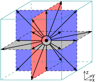
Figure 1: Visualization of a single lattice node with its $19$ stored values of the distribution functions (arrows). In one complete time step (“sweep”), all distribution functions at all lattice nodes are updated.

The performance of a given LBM approach depends at least on the data layout and memory access patterns, the strength of arithmetic operations (i. e., how well numerical expressions are simplified and combined to avoid unnecessary operations), and their degree of SIMD vectorization. A thorough overview of more propagation-step implementations and their memory access characteristics can be found in [6, 10].

It seems natural to store the PDFs in a 4-D array, and use an additional Boolean array to distinguish fluid nodes from obstacle nodes. This is known as the marker-and-cell approach. However, LBM simulations of domains with a large fraction of solid nodes can benefit from a sparse representation of the domain [1, 2, 3, 5, 8, 9], where only the fluid nodes are kept in a 1-D vector. Indirect accesses to PDFs of neighboring nodes are then required and accomplished through an adjacency list (IDX), which represents the topological connections of the nodes. ILBDC uses such a sparse representation.

For updating one node, optimized implementations read one PDF from each of the $18$ surrounding neighbors and the local node (streaming step), compute updated values (collision step), and write the results to the PDFs of the local node. This is known as the pull scheme [4]. It is implemented in the ILBDC code together with a structure-of-arrays (SoA) data layout where all PDFs of a direction are stored consecutively in memory before the next direction follows: f(i,j,k,PDF).

To work around the data dependency problems of a combined stream-collide step, two lattices are often used, one as the source and one as the destination. Then, a fluid lattice-node update (FLUP) requires $19$ PDF loads, $19$ additional PDF loads because of write-allocate (also known as fetch-on-write) transfers, $19$ PDF stores and $18$ IDX loads of the adjacency list. Assuming double-precision floating-point numbers (eight bytes) for PDF and four-byte integers for IDX, the total number of bytes that must be transferred between CPU and memory for one FLUP is $3\times 19\times 8\text{~{}(PDF)}+18\times 4\text{~{}(IDX)}$ bytes $=528$ bytes. The write-allocate is triggered by the cache hardware on store misses and loads the data at the accessed location (the complete cache line, to be exact) from memory into the cache before it is updated. With non-temporal store (NT) instructions these write-allocates are avoided and the data is directly written from the processor into memory, bypassing the cache hierarchy. The number of bytes required for one FLUP decreases then to $2\times 19\times 8\text{~{}(PDF)}+18\times 4\text{~{}(IDX)}$ bytes $=376$ bytes. Current standard processors have difficulties with $19$ concurrent write streams, in particular if they consist of NT stores. As a remedy, blocking can be applied so that a node’s PDFs are read in chunks and updated values are stored in a small temporary buffer, which should be small enough to fit in the L1 cache. From this buffer, two directions of the updated PDFs at a time are written to the destination lattice. We call this implementation pull-split T or pull-split NT, depending on whether normal (“temporal”) stores or non-temporal stores are used.

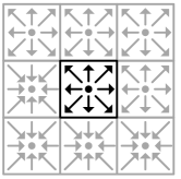
(a) Even time step: read PDFs.

(b) Even time step: write PDFs.

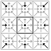
(c) Odd time step: read PDFs.

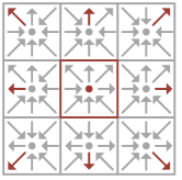
(d) Odd time step: write PDFs.

Figure 2: Visualization of the AA pattern (or propagation model), using the D$2$Q$9$ model for the sake of clarity. In the even time step of the AA pattern, only PDFs of the current node are read (a), collided, and written back to the same location (b) but into opposite directions. As a consequence, the current node PDFs are located at neighboring nodes during the following odd time step. These are then loaded from the opposing direction (c), collided, and written back (d).

Bailey’s AA pattern [7] for the PDF access allows using one single lattice only (instead of separate source and destination grids) while maintaining the possibility to update all cells in any order and in parallel. The iterations over the lattice are divided into even and odd time steps. During an even time step (Fig. 2a and 2b) only PDFs of the current node are accessed in each lattice site update. In the following odd time step (Fig. 2c and 2d) only PDFs of the neighboring nodes are accessed, which requires indirect addressing in our case of the sparse representation. This update scheme only performs stores to locations in memory which have previously been read. No write-allocate is necessary, since the data to be updated already resides in the cache. We use an optimized version where the even time step is completely SIMD-vectorizable, which can easily be accomplished as all PDFs are accessed consecutively and no indirect access is required. In the odd time step a partial vectorization is performed, which can avoid the indirect addressing and allows for vectorized execution of consecutively stored chunks of PDFs. Nodes that cannot be treated in this way are updated in the usual way without SIMD vectorization (i. e., in scalar mode). The fraction of nodes that can be updated with SIMD operations depends on the geometry used for the simulation. During even time steps, $2\times 19\times 8\text{~{}(PDF)}$ bytes $=304$ bytes per FLUP are required. In the odd time step the number of bytes needed for one FLUP depends on the fraction of vectorizable updates. The lower bound occurs when all updates can be vectorized. In this case only $2\times 19\times 8$ bytes $=304$ bytes of memory traffic are required. The upper bound is reached when all updates must be scalar and indirect accesses are needed for the adjacency information, resulting in $2\times 19\times 8\text{~{}(PDF)}+18\times 4\text{~{}(IDX)}$ bytes $=376$ bytes of traffic.

All performance-critical parts were implemented using SIMD compiler intrinsics to have full control over the code vectorization. We restrict ourselves to the SIMD instruction sets SSE4.2 (Streaming SIMD Extensions) and AVX (Advanced Vector Extensions), which are available on modern x86-based processors.

1.3 Test bed and benchmark cases

SuperMUC [25], which is installed at Leibniz Supercomputing Center (LRZ) in Garching near Munich, is a tier-0 PRACE system and one of the main federal compute resources in Germany. It is built from a number of 512-node “islands,” with a fully non-blocking fat tree FDR10 InfiniBand connectivity inside each island. A compute node comprises two Intel Sandy Bridge (“SNB”) EP (Xeon E5-2680) eight-core processors with a base clock frequency of 2.7 GHz. The actual clock speed of the processors can be set at job submission time, but the “turbo mode” feature of the Intel processors cannot be used. Consequently, all single-node benchmark tests were run on a standalone Sandy Bridge EP node with the same type of CPU and otherwise similar characteristics. Due to the ccNUMA memory architecture, the memory bandwidth scales perfectly from one to two sockets in a node.

The Intel Fortran/C compiler 13.1 and Intel MPI 4.1 were used in all cases. The operating system on SuperMUC was SuSE SLES11. Each MPI process was explicitly pinned to its physical core using sched_setaffinity() within the code. All benchmarks were run inside a single island to guarantee that communication is performed through the fully non-blocking fat tree.

Two geometries were selected for the benchmarks in this paper. The first is an empty channel which consists only of fluid nodes except for the walls. The second geometry is a packed bed reactor, i. e., a tube filled with spheres. It represents a real-world application case for flow simulation with this type of code. Both geometries have dimensions of $4000\times 80\times 80$ nodes, resulting in $25\cdot 10^{6}$ fluid nodes ($\approx 3.8$ GB lattice $+\,1.8$ GB adj. list) and $19\cdot 10^{6}$ fluid nodes ($\approx 2.9$ GB lattice $+\,1.4$ GB adj. list) for the channel and the reactor geometry, respectively.

With these dimensions both geometries fit into the NUMA locality domain of one socket on SuperMUC. For strong scaling runs the reactor geometry was enlarged to $8000\times 160\times 160$ nodes, as the smaller lattice fits in the L3 caches of $128$ compute nodes and above. The large reactor geometry consists of $157\cdot 10^{6}$ fluid nodes and requires around $24$ GB of memory for the lattice and around $11$ GB for the adjacency list.

The ILBDC code is purely MPI-parallel. All single-node measurements were thus performed with intra-node MPI only; a hybrid MPI/OpenMP version exists, but the details of the multi-threaded implementation (alignment constraints and loop peeling, encoding of obstacle-free regions for SIMD execution in the odd time step) are beyond the scope of this work. We also expect no major differences for an equivalent OpenMP-parallel version. Details about the MPI parallelization can be found in Sect. 4.1.

1.4 Contribution

This paper makes the following contributions:

The scalar and AVX-vectorized single-core performance and intra-chip saturation of an LBM implementation with AA propagation pattern are successfully described using the ECM model and compared to the popular “pull-split” propagation pattern. We show the superiority of the AA pattern in terms of performance and demonstrate that “best possible” performance is achieved on the chip.

The energy consumption of the LBM algorithm with AA propagation pattern is modeled on the chip level for a range of clock frequencies. Together with the ECM performance model, we gain a coherent picture of the performance and power properties of the LBM algorithm on the chip and achieve good qualitative agreement with measurements. A region of optimal operating points with respect to clock speed and number of cores is identified. The system’s baseline power (power consumption of everything apart from the CPUs, i. e., memory, chip sets, network, disks, etc.) is taken into account and shown to have a damping influence on the differences in energy consumption (as predicted by the power model). Even then, potential energy savings of up to 50% can be achieved compared to a naive operating point with the inferior pull-split propagation model. Single-thread code performance and the selection of an optimal number of cores per chip (the latter depending on the former) are shown to have the largest impact on energy consumption.

In highly parallel LBM runs, we observe a loss in parallel efficiency when the CPU clock speed is reduced. This unexpected result can be explained by a strong dependence of effective inter-node and intra-node MPI communication bandwidth on the clock speed. The effective bandwidth also shows a strong negative correlation with the number of MPI processes per node. As a consequence, minimal energy to solution in the highly parallel case depends even more strongly on the proper choice of the operating point, especially on the number of cores per chip (and thus the single-thread performance). A simple non-reflective reduction of the clock speed will reduce performance and may consume more energy at the same time.

2 ECM performance model

The ECM model [26, 20] is a refinement of the roofline model [27, 11]. Note that the ECM model is not specific to the lattice-Boltzmann algorithm. It has also been used successfully to describe the performance and scaling properties of streaming benchmark kernels [26, 20], stencil smoothers [28], and medical image reconstruction kernels [29]. It is to our knowledge the first approach that can successfully model the single-thread performance and on-chip scalability of data streaming applications on multicore processors.

It starts with an analysis of the serial loop instruction code to get an estimate for the “applicable peak performance,” i. e., the expected maximum performance when all data comes from the L1 cache. After that, all required data transfers needed to get the data in and out of L1 are accounted for, together with the time it takes to move the cache lines up and down through the memory hierarchy levels. Pure streaming is assumed, i. e., there are no latency effects and the prefetching mechanisms work perfectly. Since it is sometimes hard to predict which of the above contributions to the serial runtime of a loop can overlap, the ECM model generates a prediction interval based on no-overlap and full-overlap assumptions, respectively.

Modeling the in-L1 execution and data transfers both require some knowledge about the architecture, such as instruction latency and throughput, data path widths, and the achievable memory bandwidth. If some of this data is unavailable, suitable microbenchmarks or tools can be employed. Especially for the in-core performance analysis the “Intel Architecture Code Analyzer” (IACA) [30] is instrumental in getting a better view of the relevant bottlenecks. All data transfers between the memory hierarchy levels occur in packets of one cache line; hence, the ECM model always considers a “unit of work” of one cache line’s length. If, e. g., a loop accesses single precision floating-point arrays with unit stride on a CPU with 64-byte cache lines, the unit of work is sixteen iterations.

In order to predict the scaling behavior across the cores of a multi-core chip it is assumed that each core creates some bandwidth pressure on the relevant bottleneck, which is usually a shared cache or the chip’s memory interface. When the aggregate bandwidth pressure exceeds the available bandwidth, saturation sets in [31]:

$$P(t)=\min\left(nP_{0},P_{\mathrm{max}}\right)~{}.$$ (1)

Here, $n$ is the number of cores used, $P_{0}$ is the single-core performance as predicted by the ECM model, and $P_{\mathrm{max}}$ is the saturated full-chip performance for the relevant bottleneck (e. g., the memory bandwidth $b_{\mathrm{S}}$),

$$P_{\mathrm{max}}=I\cdot b_{\mathrm{S}}~{},$$ (2)

with $I$ being the computational intensity, i. e., how much “work” (flops, FLUPs, …) is done per byte transferred over the bottleneck.

2.1 Observed chip-level performance and scaling

As a motivation for doing this kind of analysis, in Fig. 3 we show the intra-socket scaling of the empty channel test case with the AA pattern for the two “extremal” clock frequencies of 2.7 GHz and 1.2 GHz, respectively, in three variants: AVX-vectorized (full 256-bit loads/stores), SSE-vectorized, and scalar.

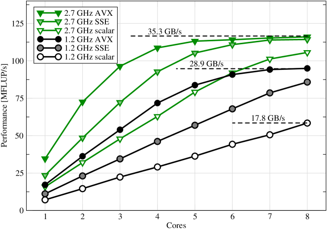
Figure 3: Intra-socket strong scaling of the AA pattern LBM implementation for an empty channel, comparing AVX, SSE, and scalar code at the clock frequencies of 2.7 GHz (triangles) and 1.2 GHz (circles). The corresponding saturated memory bandwidths are indicated for selected cases.

The data indicates that SIMD vectorization has a large impact in the serial case; in fact, the serial performance differs by more than a factor of two between the AVX and the scalar code (triangles vs. circles). At 2.7 GHz, the gap closes as the number of cores is increased. On the full socket the scalar code is hardly 10% slower than the AVX variant. The latter, however, reaches the same level already with four cores, which opens an opportunity for saving energy by leaving cores idle.

At 1.2 GHz, the situation in the serial case is similar, but on a lower level. The single-core performance of all code variants is roughly proportional to clock speed. However, only the AVX-vectorized code shows a saturation pattern, while the SSE and scalar variants scale linearly up to eight cores without reaching a bandwidth barrier. This is because these code versions do not exert sufficient “pressure” on the memory interface to reach saturation even on a full socket. Hence, lack of vectorization (“slow code”) cannot be compensated by using more cores in this case. Moreover, the maximum memory bandwidth is correlated with the core clock frequency and varies by about 20% across the full frequency range [21].

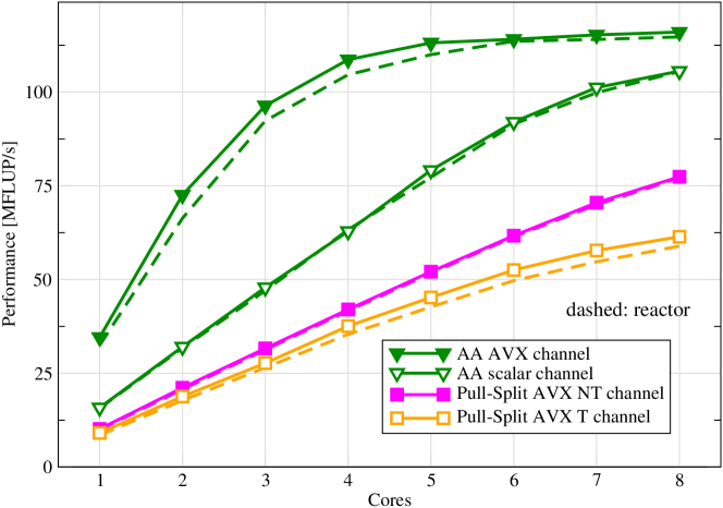
Figure 4: Intra-socket performance scaling for one SNB chip at 2.7 GHz: AA pattern in AVX and scalar variants (triangles) and pull-split pattern with AVX vectorization with (NT) and without (T) non-temporal stores (squares), for the empty channel application case (solid lines). The performance numbers for the packed reactor case are shown with dashed lines.

In Fig. 4 we show a socket-level performance comparison of the scalar and vectorized AA pattern implementation with the pull-split pattern for both application cases (empty channel vs. packed reactor) at a clock speed of 2.7 GHz. Although there is a large fraction of obstacles in the packed reactor geometry, their presence hardly influences the performance, independent of the propagation pattern. We also see that the pull-split pattern is not competitive since it is about half as fast as the scalar AA version on the single core, and there are not enough cores available to compensate for this disadvantage and reach bandwidth saturation.

The intention of applying the ECM model is to gain deeper insight into this performance behavior and to pave the way for a practically useful energy consumption analysis.

2.2 In-core analysis

An IACA throughput analysis for the AA pattern kernel shows that the ADD port of the SNB core is the sole bottleneck of core execution for all variants (scalar, SSE, AVX), as well as for even and odd time steps, and that one loop iteration (four updates with AVX, two with SSE, one for scalar) should take about 135 cycles. In contrast, a critical path analysis reports somewhat longer execution times due to dependencies in the instruction and data flow. The critical path depends on the type of time step. It has a maximum length of 163 cycles (even, AVX), 212 cycles (odd, AVX), 160 cycles (even, scalar), and 187 cycles (odd, scalar). This prediction roughly coincides with direct measurements, which we will use as an input in the following (160, 212, 158, and 160 cycles, respectively).

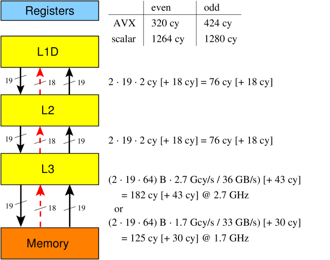
Figure 5: Single-core ECM model of the AA propagation pattern for D3Q19 LBM (eight FLUPs). Even and odd time steps have different in-core timings. One arrow represents the number of full cache line transfers indicated; dashed arrows stand for half-wide (32-byte) transfers and are required for loading the adjacency information in the odd time step when vectorization is not possible. One half-wide cache line transfer takes one cycle. Numbers in square brackets denote contributions from the adjacency list and can be ignored for the empty channel case.

These numbers must be multiplied by two (for AVX) or eight (for scalar) for getting execution times for one unit of work, i. e., a cache line. The table in Fig. 5 shows the in-core cycle counts for AVX and scalar code in the even and odd time steps, respectively.

The analysis for the packed reactor case is surprisingly very similar: The even time step does not change at all, since no index access is required. In the odd time step, even when assuming no potential for vectorization (as would be the case for an extremely porous geometry) there is ample room for hiding the additional loads for the index array due to the bottleneck on the ADD port. This step is necessarily scalar, however, so the execution time is about 4 times longer per unit of work. The actual impact of this slowdown depends on the fraction of vectorizable updates. In our applications, this fraction is roughly 97% for the empty channel and 92% for the packed reactor case. This leads to a very small performance penalty for the latter, which was already observed in Fig. 4. Hence, we will only consider the empty channel case for the rest of the chip-level analysis.

2.3 Data transfers and saturation behavior on the chip

The ECM model requires the maximum attainable memory bandwidth as an input parameter. It is known that this value depends on the number of parallel read/write streams as well as the CPU clock speed. From a data transfer perspective, the AA-pattern implementation of the D3Q19 LBM algorithm reads 19 arrays from memory, modifies their contents, and writes them back. For measuring the maximum achievable memory bandwidth on the socket, we therefore use a parallel multi-stream array update benchmark (see Listing 1).

Listing 1: Parallel multi-stream update benchmark with 19 streams. N is chosen such that the arrays do not fit in any cache. The runtime is longer than any thread creation or synchronization overhead, so this loop probes the achievable memory bandwidth independently of the programming model.

⬇

double a01[N], a02[N],..., a19[N], s=2.0;

#pragma omp parallel for

for(int i=0; i<N; ++i) {

a01[i] = s * a01[i];

a02[i] = s * a02[i];

...

a19[i] = s * a19[i];

}

It is designed to mimic the data streaming behavior of the LBM algorithm. Care is taken to ensure that the compiler generates the “intended” assembly code, i. e., full-width aligned AVX loads/stores are used and loop splitting is avoided. Note that the benchmark in Listing 1 uses OpenMP, but our LBM code is MPI-only. This difference is insignificant here because the benchmark serves as a pure bandwidth probe: any OpenMP-related overhead, such as thread creation and barrier synchronization, is orders of magnitude smaller than the runtime of the loop.

Figure 6 shows the achieved memory bandwidth on one SNB socket with varying number of threads (cores) and clock frequencies between 1.2 GHz and 2.7 GHz (plus turbo mode). As predicted by the ECM model, the single-thread performance is proportional to the clock speed and the saturation point is shifted to larger thread counts as the clock speed decreases: while saturation is reached near three cores with turbo mode, up to six cores are needed at the lowest frequencies. Due to the large number of read/write streams, the maximum bandwidth is significantly lower than with a standard single-stream update kernel (dashed line in Fig. 6). At the same time, the maximum (saturation) memory bandwidth drops by about 25% over the whole frequency range; there is another substantial drop when using the full socket (eight cores) at the lowest frequency. As of now we have no conclusive explanation for these latter effects. They do, however, influence the considerations on energy dissipation, which will be discussed in Sect. 3.

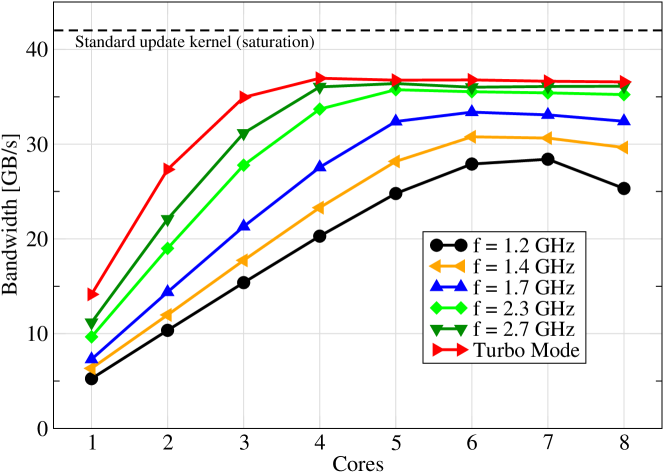
Figure 6: Multi-stream update benchmark performance scaling on one SNB socket with different CPU frequency settings. 19 update streams were run per thread. The dashed line indicates the maximum achievable bandwidth with a simple single-array update kernel.

In the following we will use the maximum bandwidths as measured at the respective frequencies as an input to the ECM model in order to calculate the number of cycles required to transfer cache lines between memory and L3 cache.

Fig. 5 shows the complete ECM model analysis at 2.7 and 1.7 GHz, respectively. The cycle counts in square brackets are contributions from loading the adjacency information (dashed arrows), and can be ignored for the empty channel case. The achievable memory bandwidth (36 GB/s and 33 GB/s, respectively) and the clock speed enter the model when calculating the cycles for data transfers to and from main memory. Data transfers between adjacent cache levels are assumed occur at 32 bytes per cycle, so these cycle counts are independent of the clock frequency. The various execution and data transfer times may be combined in different ways to arrive at a performance prediction for the serial program:

1. The most conservative (worst case) assumption is that none of those contributions overlap with each other, so that the execution time is equal to their sum (e. g., 320+2$\cdot$76+182=654 cycles for the even time step with AVX at 2.7 GHz).

2. The most optimistic assumption is that the cycles in which the L1 cache is occupied by loads and stores from the core cannot be used for reloads and evicts to L2, but all other contributions do overlap.

3. Lastly one may assume that the pure in-core execution part (everything except loads and stores) can overlap with loads and evicts from/to the L2 cache, but that there is no overlap beyond that.

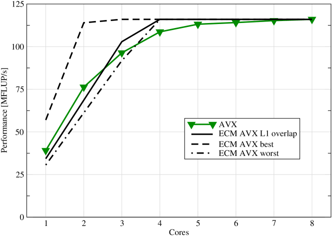
Figure 7: Performance of the AVX (triangles) implementation of the LBM algorithm with AA propagation (empty channel case) at 2.7 GHz. The ECM model predictions for AVX with full overlap assumption (dashed line), no overlap (dotted-dashed line), and partial overlap at L1 (solid line) are shown for comparison.

None of these assumptions coincides with the roofline model, which requires the achievable memory bandwidth for each number of cores as an input parameter. The ECM model only requires the maximum (saturated) bandwidth and it predicts the scaling.

2.4 Validation of the performance model

Figure 7 shows a comparison of the measured performance for the AVX-vectorized AA pattern implementation with the three models described above. Apart from the region around the saturation point (3–4 cores), the third assumption provides the best fit to the data.

It was already shown in Fig. 4 that the pull-split propagation pattern (with and without NT stores) is not competitive since it cannot saturate the memory bandwidth, although the NT version has almost the same computational intensity as the AA pattern. This failure can mainly be attributed to the fact that the pull-split variant cannot be efficiently SIMD-vectorized on the Sandy Bridge architecture due to the indirect access in every lattice site update. More specifically, the loop which loads the neighboring distribution functions and stores intermediate results into temporary buffers is scalar. We will thus ignore pull-split from now on and focus the following discussion on the AA pattern.

3 Power model

Recently, considerations of power dissipation and energy to solution have received much interest in the supercomputing community. The two prevalent questions are: (i) “How can a parallel code be run so that its overall energy consumption until a solution is reached can be minimized, preferably under the constraint of constant time to solution?” and (ii) “How can a parallel computer be operated in a production environment so that overall power dissipation is minimized or kept below a given maximum?”

We concentrate on the first question here. In [20] we have established a simple power model which is able to explain many of the peculiar properties of the energy-to-solution metric on a multicore processor for load-balanced codes that may show some performance saturation as the number of cores used is increased. In the following, we briefly summarize its derivation and the most important conclusions drawn from it.

3.1 Power versus clock speed and energy to solution

Direct measurements on the Sandy Bridge chip [20] with the RAPL interface [32, 33] and the likwid-powermeter tool show an expected strong growth of power dissipation with rising clock frequency. Although it is not clear what the actual dependence should be, measurements suggest a power law with an exponent between 1 and 3 [20]. This is presumably due to a hard-wired, chip-specific mapping of the clock speed setting to the core supply voltage. Motivated by measurements on a variety of current Intel processor models, we assume a quadratic behavior so that the power dissipation is

$$W(f,n)=W_{0}+\left(W_{1}f+W_{2}f^{2}\right)n~{},$$ (3)

where $f$ is the clock frequency and $n$ is the number of active cores. The part which is linear in $n$ is the dynamic power dissipation, whereas $W_{0}$ is the baseline power. $W_{0}$ may include contributions from the rest of the system, such as memory, I/O circuitry, network, disks, and cooling. The parameters $W_{1}$ and $W_{2}$ characterize the interaction of the code with the hardware in terms of energy consumption, and they depend on the code being executed and on the data transfers through the cache hierarchy. They vary by no more than a factor of two even across very different code characteristics on the CPU considered here [20] and can be determined by direct measurements at different clock speeds. Here we choose $W_{2}\approx 1\,\mbox{W}/\mbox{GHz}^{2}$, $W_{0}\approx 23\,\mbox{W}$ for the chip level, and $W_{0}\approx 73\,\mbox{W}$ for the per-socket share of the whole system. Note that we do not expect these values to be exact (they even vary across multiple specimens of the same processor type), but they are sufficient for a qualitative analysis. Since $W_{1}$ is very small on the processors considered here, we neglect it in the following.

Energy to solution is proportional to the ratio of power dissipation to performance (for a constant problem). We assume that multi-core performance can be modeled by

$$P(t)=\min\left(\frac{f}{f_{0}}\,nP_{0},P_{\mathrm{max}}\right)~{},$$ (4)

where $f_{0}$ is the base (“nominal”) frequency of the chip, $P_{0}$ is the serial performance at $f_{0}$, $n$ is the number of active cores, and $P_{\mathrm{max}}$ is a maximum performance (see also Sect. 2). $P_{\mathrm{max}}$ may be set by the presence of some bottleneck such as the memory bandwidth, or it may be infinite if the code is perfectly scalable. Hence, the energy to solution is

$$E=\frac{W_{0}+W_{2}f^{2}n}{\min\left(\frac{f}{f_{0}}\,nP_{0},P_{\mathrm{max}}\right)}~{}.$$ (5)

The “roofline model of energy” by Choi et al. [22] also uses direct power measurements and microbenchmarks to fix model parameters such as the cost for a data transfer or for a floating-point operation, but it does not address frequency dependence and multicore scaling, and it reduces the code characteristics to a single number (computational intensity). These properties make it very useful for comparisons between architectures and for design space exploration, while our model is more phenomenological. Still the method from [22] could be used to determine or at least estimate $W_{0}$, $W_{1}$, and $W_{2}$.

It is a simple consequence from this model that a minimum energy to solution is reached near the performance saturation point, i. e., at the smallest number of cores $n$ for which $P(n)=P_{\mathrm{max}}$. If by some means $P_{\mathrm{max}}$ can be increased, e. g., by choosing the AA propagation pattern, energy to solution will immediately go down proportionally. In case the available number of cores is too small to get saturation, i. e., if the performance scales well, all cores must be used for minimum energy consumption.

The single-core performance $P_{0}$ also appears only in the denominator. In the application cases we consider here, it is mainly influenced by the SIMD vectorization and thus, indirectly, by the choice of propagation pattern. The larger $P_{0}$, the fewer cores are needed to reach saturation, so there is an inherent energy saving potential in having a fast single-threaded code.

The dependence of $E$ on the clock frequency is more complex: If there is no saturation there may be an optimal frequency $f_{\mathrm{opt}}$ for which $E$ is minimal:

$$f_{\mathrm{opt}}=\sqrt{\frac{W_{0}}{W_{2}n}}$$ (6)

If $W_{0}$ comprises only the chip’s idle power, $f_{\mathrm{opt}}$ is in the range of accessible frequencies. However, a low frequency setting has the adverse effect of extending the time to solution, which may not be desirable. Cost models other than time or energy (such as the energy-delay product) may then be needed to determine whether this is acceptable. On the other hand, if $W_{0}$ contains (the chip’s share of) the baseline power of the complete node, $f_{\mathrm{opt}}$ is usually near or beyond the highest possible setting. We call this “clock race to idle,” because a fast clock speed saves energy. The details of this analysis can be found in [20].

3.2 Energy to solution for the LBM solver on the chip

The ECM model and the power model enable a combined analysis of the energy and performance properties of the LBM algorithm. It is useful to plot energy to solution versus performance, with the number of cores used as a parameter within a data set for a specific frequency, SIMD vectorization variant, propagation method, or any other property.

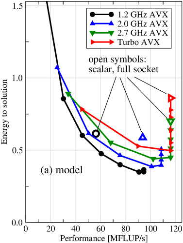
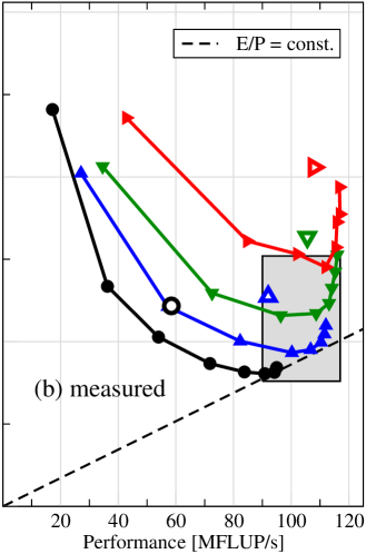
Figure 8: Energy to solution vs. performance of the AVX-vectorized LBM AA pattern implementation (empty channel case) of one SNB socket for different clock frequencies (lines and filled symbols). The number of cores used (processes per chip, PPC) is the parameter along each data set. (a) Predictions by the ECM performance model and the chip-level power model. (b) Measured data. For comparison, the big open symbols mark the energy and performance of the scalar code on a full socket. The shaded area is the region defined by absolute minimum energy and saturated performance for the AVX versions. The dashed line is the line of constant energy-delay product that hits the saturation point of the lowest-frequency run. Note that all legends in (a) also apply to (b).

This has been done in Fig. 8a for three different clock frequencies and turbo mode, using the AA pattern in the AVX variant (filled symbols). For comparison we also show the energy-performance data for full socket runs with purely scalar code (large open symbols). In turbo mode, each data point was computed using the maximum allowed frequency for each number of active cores. The corresponding measurements are shown in Fig 8b. Note that we always show energy to solution in arbitrary units, but the values shown are coherent for a specific problem size (geometry and number of iterations).

The models are able to describe the qualitative features of energy and performance. The observed deviations are caused by (i) the inability of the ECM model to accurately describe the performance behavior in the vicinity of the saturation point, (ii) the inaccuracy in determining $W_{2}$ and $W_{0}$, and (iii) the approximation of linear power behavior with respect to core count even with saturated codes like LBM at higher clock speeds. In addition, turbo mode does not fit perfectly into the model (5) since the SNB chip can operate beyond its thermal design power (TDP) for a limited amount of time [33]. This is why the deviation from the measurements is especially large with turbo mode (right-pointing triangles in Fig. 8).

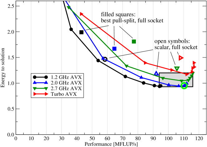
Figure 9: Same data as in Fig. 8b but with a realistic per-socket baseline power of $W_{0}^{\prime}=W_{0}+50\,\mbox{W}=73\,\mbox{W}$. The circle marks a possible optimal operating point for almost minimal energy with a tolerable loss in performance. For reference, the best data for the pull-split propagation pattern (vectorized, full socket) for 1.2, 2.0, and 2.7 GHz is also shown (filled squares).

Scalar code (large open symbols) is only able to (almost) saturate the memory bandwidth at 2.7 GHz, and it is neither competitive in the energy nor in the performance dimension. Looking at the minimum energy point with respect to clock frequency and number of cores in the regime where performance is not saturated, we see that this point moves to smaller frequency as the core count goes up, as described by Eq. (6). In general, a faster sequential code (AVX instead of scalar) saves energy. Comparing energy to solution for the AVX codes at their respective saturation points, we can identify an “optimization space” (shaded area in Fig. 8b), in which the desired optimal operating point should be found. Depending on the emphasis one wants to put on energy minimization vs. maximum performance, this point may be in the lower left corner of the area. In this case one would use all cores at the lowest frequency (1.2 GHz, filled circles) and sacrifice about 20% of performance compared to the right edge of the area, which is defined by the saturation point at higher frequencies (2.0 GHz to turbo mode). Another clear conclusion is that turbo mode is of no good use for the LBM implementations studied here, neither from a performance nor from an energy point of view.

There is no single, well-defined criterion for identifying the optimal operating point on the chip level. One may certainly employ cost models such as the energy-delay product (ratio of energy and performance), but this is only one possible choice. For reference we have included a line of constant energy-delay product in Fig. 8b. From the data we have collected, using 5–6 cores at 2.0–2.3 GHz seems to provide a good compromise between performance loss and energy consumption (“as far on the lower right as possible”).

While the model and the measurements yield a consistent picture on the chip level, it is clear that the chip contributes only a (however significant) part to the overall power consumption of a compute node. As mentioned above, the rest of the system should be taken into account when assessing the real energy demand for running an application. We do this by adding an extra, constant contribution of 50 W to the chip-level baseline power, so that the new baseline power is $W_{0}^{\prime}=23\,\mbox{W}+50\,\mbox{W}=73\,\mbox{W}$. This leads to roughly 300 W of maximum node power (assuming two-socket nodes and a maximum power dissipation per socket of 100 W), which is the value measured during a LINPACK run on SuperMUC [34]. With this change we can offset the energy measurements from Fig. 8 to arrive at the data shown in Fig. 9. Note that the modified baseline $W_{0}^{\prime}$ also contains everything beyond the chip, especially including the network and the cooling infrastructure, broken down to the socket level. We thus assume that these contributions are largely constant compared to the dynamic power variations parametrized by $W_{2}$, $f$, and $n$ in Eq. (5).

As expected, the modified baseline power leads to a reduction of the vertical spread between the measurements for different clock frequencies. While it was possible with the chip-level (i. e., small) $W_{0}$ to have a situation where energy to solution was heavily influenced by frequency and SIMD vectorization even at a specific performance level (with a spread of up to 2$\times$ within the optimization space shown in Fig. 8), the large $W_{0}^{\prime}$ reduces the spread to about 25%. Hence, a large baseline power favors the “race to idle” principle where the most influential parameter is performance; optimizations that favor a larger saturation performance (such as the AA propagation pattern or blocking schemes which increase the computational intensity) have the most potential for saving energy. In addition, optimized clock speed and a reduction of the number of cores used can yield second-order but still significant savings. Within the transformed optimization space (shaded area in Fig. 9) we can identify a possible optimal operating point at about 2.0 GHz and six cores, with almost minimal energy to solution and a performance loss of about 6% compared to the highest possible saturation level. In comparison to a naive strategy of running on all cores with turbo mode enabled and a scalar kernel, more than one third of the energy can be saved.

The “race to idle” principle with respect to maximum code performance is evident from a comparison with the energy-performance data for the pull-split pattern (filled squares) in the best variant (SSE or AVX vectorized, non-temporal stores, full socket) at three different frequencies in Fig. 9: The pull-split pattern can neither compete with AA in the performance nor in the energy dimension. Using AA, almost a factor of two in energy and 30–40% of runtime can be saved in comparison to pull-split.

4 MPI-parallel LBM simulations

4.1 MPI parallelization in ILBDC

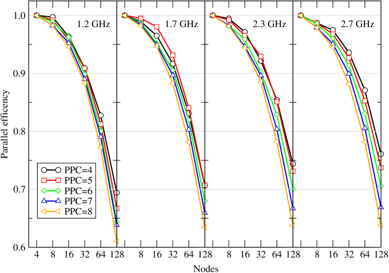
Figure 10: Parallel efficiency of the large packed bed reactor application case ($8000\times 160\times 160$ lattice nodes) for different frequency settings and different number of processes per chip (PPC) on up to 128 nodes of SuperMUC. The efficiency calculation was based on the four-node performance baseline.

ILBDC uses an MPI parallelization with a static load balancing scheme. The sparse representation of the lattice is cut into equally sized chunks, so that each MPI rank receives the same number of fluid nodes. The interfaces of such generated partitions can be arbitrarily formed with different numbers of partition neighbors, as the simple cutting of the sparse representation does not consider any topological information. However, in the case of the channel and reactor benchmark geometries this method results only in a 1-D decomposition, where each rank only needs to exchange ghost PDFs with its two direct neighbors. We distribute the ranks linearly across the compute nodes, so that consecutive ranks are located nearby on the same node. Due to the implicit one-dimensional domain decomposition, only the first and the last rank on a compute node must then perform inter-node communication. All the remaining ranks communicate within the node only. For the same reason, in case of strong scaling the communication volume of each process stays constant when the number of processes goes up: each rank gets a successively smaller slice of the long geometries.

The packed bed reactor geometry was used for all the multi-node experiments, since it is the application scenario that is relevant in practice. We have shown earlier that the node-level performance (and thus power) properties are very similar to the empty channel case. Note also that “turbo mode” cannot be activated on SuperMUC, so we stick to the fixed frequencies of 1.2, 1.7, 2.3, and 2.7 GHz in the following.

4.2 Performance and energy at strong scaling

4.2.1 Parallel efficiency and communication performance

All variants of the AA pattern scale well up to 32 nodes (512 cores) at all frequencies and parallel efficiency only starts to degrade below 90% beyond that point. Scaling experiments were performed on up to 128 nodes (2048 cores), since this is where some variants start to show efficiencies as low as 60%. In Fig. 10 we show the parallel efficiency of the strong scaling runs versus the number of nodes at the four chosen frequencies and with between four and eight processors per chip (PPC). Since the application case is too large to fit on a single node, all efficiency numbers were normalized to the four-node run.

Usually one would expect the parallel efficiency to increase as the node-level performance goes down, because communication and synchronization overheads become less important when the pure compute time goes up. On SuperMUC, the opposite is the case: the minimum parallel efficiency (at 128 nodes) varies between 76 and 63% (depending on the number of processes per chip) for 2.7 GHz, but between 69 and 61% at 1.2 GHz. We conclude that there must be a frequency-dependent factor which impedes scalability whenever communication overhead plays a significant role.

In order to explore the reasons for this effect we have conducted experiments with “sendrecv” from the Intel MPI benchmark suite (IMB) [35], since it mimics the ringshift-like halo-exchange communication pattern of the ILBDC code. Each MPI process exchanges data with its neighbors: MPI_Sendrecv(to right neighbor, from left neighbor). The benchmark reports the available communication bandwidth per process. In Fig. 11 we show the results for two SuperMUC nodes in the two corner cases of one process (PPN=1) and 16 processes per node (PPN=16) for the two extremal frequencies of 1.2 and 2.7 GHz. The placement of the MPI ranks was done in the same way as for the ILBDC benchmarks: neighboring ranks were “packed” to the same node to minimize inter-node traffic.

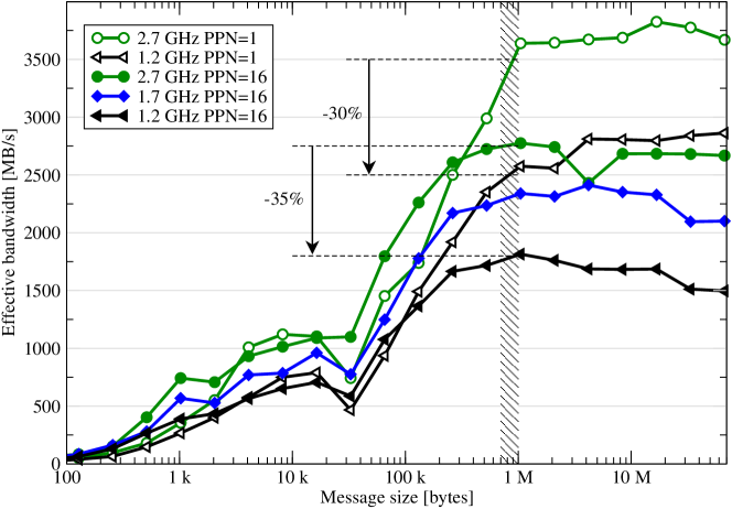
Figure 11: IMB sendrecv benchmark results on two SuperMUC nodes for different CPU clock speed settings with 16 processes per node (filled symbols) and one process per node (open symbols). The mapping of MPI ranks to cores was set for minimum inter-node traffic (consecutive ranks on the cores of a node). The shaded area indicates the range of message sizes for the LBM application test case (packed bed reactor geometry). The effective communication bandwidth drops by 35% across the available frequency range at PPN=16 and still by 30% at PPN=1 (arrows).

Although both scenarios show a dependence of the effective MPI bandwidth on the clock speed, this is especially pronounced at PPN=16, and we see a breakdown of about 35% in communication bandwidth within the region of message sizes relevant for the ILBDC packed reactor benchmark (shaded area). Moreover, the bandwidth of the FDR-10 IB interface cannot be saturated even at the highest frequency setting with PPN=16. We attribute both effects to the dominance of intra-node communication, which has a strong dependence on clock speed. In contrast, the saturated LBM performance with the AA pattern and AVX vectorization only drops by about 20% over the whole frequency range (see Fig. 3). This explains the stronger breakdown of parallel efficiency at strong scaling and low clock speeds.

4.2.2 Energy and performance at scale

The question remains whether one can extrapolate the findings about energy to solution and performance from the chip to the multi-node level and especially whether single-core optimizations, notably SIMD vectorization, have a similar impact. Figure 12 shows aggregated socket-level energy (as measured via RAPL) vs. performance with AVX for the three node counts (32, 64, and 128) at which parallel efficiency is between 90 and 60%. Along each curve, the number of processes per chip (PPC) is increased from four to eight, and the highest energy point at the top of each curve is at PPC=8. For reference we also show the corresponding lowest-energy data points for the scalar implementation (open symbols).

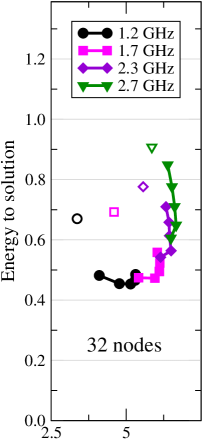
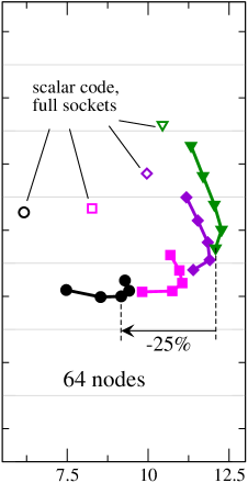
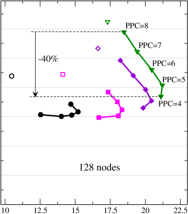
Performance [GFLUP/s]

Figure 12: Multi-node energy to solution vs. performance for the AA pattern AVX LBM implementation (large reactor case) for different clock speeds and different node counts. The parameter along each curve is the number of processes per chip (4 … 8). For comparison, the open symbols show data for the scalar implementation on full sockets. Note the overlapping scales on the three graphs. The chip-only baseline power of $W_{0}=23\,\mbox{W}$ was assumed per socket.

The overall rise in energy to solution with growing node count is a trivial consequence of the decreasing parallel efficiency, because more parallelism means more overhead. From the data it appears as if a possible optimal operating point were at 64 nodes, $f=1.2\,\mbox{GHz}$, and six cores per chip. However, performance is about 25% lower than at $f=2.7\,\mbox{GHz}$ with PPC=6 at this node count (see arrow), so the time to solution is 33% larger. This trade-off can only be investigated by looking at metrics beyond pure energy to solution, such as the energy-delay product or related approaches [17, 18]. Which metric should be chosen depends on local policies, of course, and is out of scope for this work.

The most striking difference to the chip-level results is the notable performance degradation after the saturation point, especially at the larger node counts (64 and 128). It is caused by the drop in ringshift bandwidth (as described in the previous section) with growing PPC and directly leads to a fast rise in energy to solution, much steeper than would be expected by the power model without communication component. Hence, it is even more crucial in the highly parallel case to select the optimal operating point, since each expendable core costs an over-proportional amount of energy: at 128 nodes and 2.7 GHz, the reduction in energy consumption when going from the full socket (at PPC=8 with 18.5 GFLUP/s) to the saturation point (at PPC=4 with 21.1 GFLUP/s) is over 40% (see arrow), but only about 25% on a single chip (see the 2.7 GHz data in Fig. 8b).

The strong disadvantage of scalar execution can also be seen on the highly parallel level (open symbols in Fig. 12 show the “naive” operating point of PPC=8 for this case). Since more processes are needed to reach saturation – if this is possible at all –, the slowdown at larger PPC contributes strongly to the low performance and high energy consumption. As a consequence, a well-vectorized LBM code is instrumental for optimal energy to solution, particularly in the highly parallel case when communication plays a noticeable (but not dominant) role.

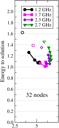
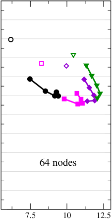
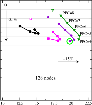
Performance [GFLUP/s]

Figure 13: Same data as in Fig. 12 but with a realistic baseline power of $W_{0}^{\prime}=73\,\mbox{W}$ per socket. The green circle marks a possible optimal operating point.

Finally, we need to comment on how these findings change if a realistic baseline power is used. Figure 13 shows the same data as Fig. 12 but with the modified per-socket baseline power of $W_{0}^{\prime}=73\,\mbox{W}$ (see Sect. 3.2). The results are very similar to the chip-level discussion: Time to solution becomes more important as the main influencing factor for energy consumption. All differences are damped by the larger idle power, but at 128 nodes there is still about 35% gain between a naive scalar code run with PPC=8 on full sockets (open green triangle) and the possible optimal operating point, which is marked in Fig. 13) at PPC=4 and 2.3 GHz. In contrast to the case where only the bare chip baseline power of $W_{0}=23\,\mbox{W}$ is considered, the lowest frequency setting of 1.2 GHz is very unfavorable, not only in terms of performance but also in terms of energy: the large performance degradation, the communication bandwidth breakdown problem, and the large baseline power combined prohibit the use of very small frequencies, even if energy to solution were the only relevant metric. On the other hand, energy is practically constant between 1.7 GHz and 2.7 GHz when the best PPC value is chosen (PPC=4 at 2.7 GHZ, PPC=4 (or 5) at 2.3 GHz, and PPC=5 (or 6) at 1.7 GHz), but performance is boosted by 15% at 128 nodes (from 18.3 GFLUP/s to 21.1 GFLUP/s). Hence, when the operating point is carefully chosen, it is possible to trade cores for performance at almost constant energy to solution by increasing the clock speed and reducing the number of cores at the same time.

5 Summary and outlook

We have analyzed the performance and energy to solution properties of a lattice-Boltzmann flow solver on the chip and highly parallel levels for an Intel Sandy Bridge EP-based system. Different propagation patterns (pull-split vs. AA), SIMD vectorization schemes (scalar vs. SSE/AVX), and the dependence on the clock speed of the processors and the number of processes per chip were explained using the chip-level ECM performance model and a simple power model. In addition to the measured chip power, the (estimated) “true” system-level power was taken into account in order to arrive at useful predictions for realistic scenarios. The power model describes well the general chip-level behavior of the energy to solution metric with bandwidth-limited loop code: (i) Minimum energy to solution is achieved at the saturation point. (ii) Lowering the frequency leads to better scalability across cores and the saturation point is shifted to larger core counts. (iii) Improved serial performance leads to fewer cores required to reach saturation.

Since the LBM algorithm and implementation used here is bandwidth-limited if properly optimized, we found a high single-core performance to be the pivotal instrument for reaching minimal energy without sacrificing too much time to solution. AVX vectorization and the choice of a good propagation pattern are important components for accomplishing this goal. Technical measures such as clock speed reduction have less impact but still contribute considerably to the overall energy consumption.

When a “good” single-core code has been found and the optimal clock speed has been set, it is the identification of the performance saturation point with respect to the number of processes on the chip level, but more importantly in the highly parallel case, which decides upon minimal energy to solution. Due to the MPI communication adding a strongly frequency-dependent component to execution time, using too many cores per chip must be avoided when communication plays a non-negligible role.

The impact of the whole system’s baseline power consumption (i. e., powered on but with idle cores) is twofold: it attenuates the differences in energy to solution caused by technical measures such as clock speed adjustments, but it emphasizes the influence of bare chip-level performance and communication overhead, especially in the highly parallel case. Hence, a combination of “good” single-chip code, a correct choice of active cores, and an optimal clock speed is needed when dealing with a realistic scenario, i. e., full-system power consumption and parallel production runs. As a consequence, a simple, possibly automatic reduction of the clock speed (triggered by the observed strong memory bandwidth utilization) may only yield a very small fraction of the potential energy savings compared to a setting in which all parameters are chosen optimally.

These results should be generalizable to any memory-bound algorithm whose communication overhead becomes significant at strong scaling, if the behavior of the basic performance-limiting parameters is similar to the system used in our analysis (SuperMUC). Specifically, the effective communication bandwidth has to depend more strongly on the clock speed than the memory bandwidth.

This work opens the possibility for future research in multiple directions. We have not addressed realistic alternatives to the standard quality metrics of energy and time to solution in detail. One such cost function could be the energy-delay product or one of its variants, but there may be others. Moreover it will be interesting to compare our findings for a typical x86-based cluster to a modern low-power system such as the IBM Blue Gene/Q. Power capping is an additional operational constraint of modern systems and can be studied using the same methods as shown here. Lastly, the ECM model and the multicore power model need refinements and adjustments to be able to deal with more complex hardware and software scenarios such as the expected flexible (per-core) frequency settings on upcoming Intel processors. Also it would be worthwhile to explore the reasons for the deviation of the ECM model from measurements near the saturation point, which does not occur for all types of code [20].

References

- [1] M. Schulz, M. Krafczyk, J. Tölke and E. Rank. Parallelization strategies and efficiency of CFD computations in complex geometries using lattice Boltzmann methods on high performance computers. In: M. Breuer, F. Durst and C. Zenger (eds.), High Performance Scientific and Engineering Computing Proceedings of the 3rd International FORTWIHR Conference on HPSEC, Erlangen, March 12-14, 2001, vol. 21 of Lecture Notes in Computational Science and Engineering (Springer, Berlin, Heidelberg), 115–122. DOI:10.1016/j.jcp.2008.01.013.
- [2] C. Pan, J. F. Prins and C. T. Miller. A high-performance lattice Boltzmann implementation to model flow in porous media. Computer Physics Communications 158(2), (2004) 89–105. DOI:10.1016/j.cpc.2003.12.003.
- [3] J. Wang, X. Zhang, A. G. Bengough and J. W. Crawford. Domain-decomposition method for parallel lattice Boltzmann simulation of incompressible flow in porous media. Phys. Rev. E 72(1), (2005) 016706. DOI:10.1103/PhysRevE.72.016706.
- [4] G. Wellein, T. Zeiser, S. Donath and G. Hager. On the single processor performance of simple lattice Boltzmann kernels. Computers & Fluids 35, (2006) 910–919. DOI:10.1016/j.compfluid.2005.02.008.
- [5] M. Bernaschi, S. Succi, M. Fyta, E. Kaxiras, S. Melchionna and J. Sircar. MUPHY: A parallel high performance MUlti PHYsics/Scale code. In: IEEE International Symposium on Parallel and Distributed Processing, 2008. IPDPS 2008. 1–8. DOI:10.1109/IPDPS.2008.4536464.
- [6] K. Mattila, J. Hyvaluoma, J. Timonen and T. Rossi. Comparison of implementations of the lattice-Boltzmann method. Computers & Mathematics with Applications 55(7), (2008) 1514–1524. DOI:10.1016/j.camwa.2007.08.001.
- [7] P. Bailey, J. Myre, S. Walsh, D. Lilja and M. Saar. Accelerating lattice Boltzmann fluid flow simulations using graphics processors. In: International Conference on Parallel Processing 2009 (ICPP’09). 550–557. DOI:10.1109/ICPP.2009.38.
- [8] D. Vidal, R. Roy and F. Bertrand. On improving the performance of large parallel lattice Boltzmann flow simulations in heterogeneous porous media. Computers & Fluids 39(2), (2010) 324–337. DOI:10.1016/j.compfluid.2009.09.011.
-
[9]
J. Zudrop, H. Klimach, M. Hasert, K. Masilamani and S. Roller.
A fully distributed CFD framework for massively parallel
systems.
In: Cray Users Group Conference 2011, Stuttgart, Germany.
https://cug.org/proceedings/attendee_program_cug2012/in%cludes/files/pap136.pdf - [10] M. Wittmann, T. Zeiser, G. Hager and G. Wellein. Comparison of different propagation steps for lattice Boltzmann methods. Computers & Mathematics with Applications 65(6), (2013) 924–935. DOI:10.1016/j.camwa.2012.05.002.
- [11] S. Williams, A. Waterman and D. Patterson. Roofline: an insightful visual performance model for multicore architectures. Commun. ACM 52(4), (2009) 65–76. DOI:10.1145/1498765.1498785.
- [12] A. Peters, S. Melchionna, E. Kaxiras, J. Lätt, J. K. Sircar, M. Bernaschi, M. Bisson and S. Succi. Multiscale simulation of cardiovascular flows on the IBM Bluegene/P: Full heart-circulation system at red-blood cell resolution. In: Proceedings of the ACM/IEEE International Conference for High Performance Computing, Networking and Storage, SC 2010, New Orleans, LA, USA, November 13-19, 2010 (IEEE), 1–10. DOI:10.1109/SC.2010.33.
- [13] J. Carter, M. Soe, L. Oliker, Y. Tsuda, G.Vahala, L. Vahala and A. Macnab. Magnetohydrodynamic turbulence simulations on the earth simulator using the lattice Boltzmann method. In: Proceedings of the ACM/IEEE International Conference for High Performance Computing, Networking and Storage (SC05), Seattle, WA, November 12-18, 2005.
- [14] S. Williams, J. Carter, L. Oliker, J. Shalf and K. Yelick. Optimization of a lattice Boltzmann computation on state-of-the-art multicore platforms. J. Parallel Distrib. Comput. 69(9), (2009) 762–777. DOI:10.1016/j.jpdc.2009.04.002.
-
[15]
V. Keller.
Energy-to-solution: a today’s metric for tomorrow’s concerns.
Talk at the Symposium on Future Generations of Processors and Systems
(FGPS’175), University of Mons, November 9th, 2012.
http://www.ig.fpms.ac.be/sites/default/files/FGPS175-Ke%%****␣sc13lbm.bbl␣Line␣125␣****ller.pdf - [16] A. Bode. Energy to solution: A new mission for parallel computing. In: F. Wolf, B. Mohr and D. Mey (eds.), Euro-Par 2013 Parallel Processing, vol. 8097 of Lecture Notes in Computer Science (Springer Berlin Heidelberg). ISBN 978-3-642-40046-9, 1–2. DOI:10.1007/978-3-642-40047-6_1.
- [17] C. Bekas and A. Curioni. A new energy aware performance metric. Computer Science – Research and Development 25(3-4), (2010) 187–195. ISSN 1865-2034. DOI:10.1007/s00450-010-0119-z.
- [18] C.-H. Hsu, J. A. Kuehn and S. W. Poole. Towards efficient supercomputing: Searching for the right efficiency metric. In: Proceedings of the 3rd ACM/SPEC International Conference on Performance Engineering, ICPE ’12 (ACM, New York, NY, USA). ISBN 978-1-4503-1202-8, 157–162. DOI:10.1145/2188286.2188309.
- [19] D. Li, B. R. de Supinski, M. Schulz, D. S. Nikolopoulos and K. W. Cameron. Strategies for energy efficient resource management of hybrid programming models. IEEE Transactions on Parallel and Distributed Systems 99. DOI:10.1109/TPDS.2012.95.
- [20] G. Hager, J. Treibig, J. Habich and G. Wellein. Exploring performance and power properties of modern multicore chips via simple machine models. Concurrency Computat.: Pract. Exper. DOI:10.1002/cpe.3180.
-
[21]
R. Schöne, D. Hackenberg and D. Molka.
Memory performance at reduced CPU clock speeds: an analysis
of current x86-64 processors.
In: Proceedings of the 2012 USENIX conference on Power-Aware
Computing and Systems, HotPower’12 (USENIX Association, Berkeley, CA, USA).
https://www.usenix.org/system/files/conference/hotpower%12/hotpower12-final5.pdf - [22] J. W. Choi, D. Bedard, R. Fowler and R. Vuduc. A roofline model of energy. In: Parallel Distributed Processing (IPDPS), 2013 IEEE 27th International Symposium on. 661–672. DOI:10.1109/IPDPS.2013.77.
- [23] T. Zeiser, G. Hager and G. Wellein. Benchmark analysis and application results for lattice Boltzmann simulations on NEC SX vector and Intel Nehalem systems. Parallel Processing Letters 19(4), (2009) 491–511. DOI:10.1142/S0129626409000389.
- [24] I. Ginzburg, F. Verhaeghe and D. d’Humieres. Two-relaxation-time lattice Boltzmann scheme: About parametrization, velocity, pressure and mixed boundary conditions. Commun. Comput. Phys. 3(2), (2008) 427–428.
-
[25]
SuperMUC petascale system.
http://www.lrz.de/services/compute/supermuc - [26] J. Treibig and G. Hager. Introducing a performance model for bandwidth-limited loop kernels. In: Proceedings of the Workshop Memory issues on Multi- and Manycore Platforms at PPAM 2009, the 8th International Conference on Parallel Processing and Applied Mathematics, vol. 6067 of Lecture Notes in Computer Science (Springer, Wroclaw Poland), 615–624. DOI:10.1007/978-3-642-14390-8_64.
-
[27]
W. Schönauer.
Scientific Supercomputing: Architecture and Use of Shared and
Distributed Memory Parallel Computers (Self-edition), 2000.
http://www.rz.uni-karlsruhe.de/~rx03/book - [28] M. Wittmann, G. Hager, J. Treibig and G. Wellein. Leveraging shared caches for parallel temporal blocking of stencil codes on multicore processors and clusters. Parallel Processing Letters 20(4), (2010) 359–376. DOI:10.1142/S0129626410000296.
- [29] J. Treibig, G. Hager, H. G. Hofmann, J. Hornegger and G. Wellein. Pushing the limits for medical image reconstruction on recent standard multicore processors. Int. J. High Perform. Comp. Appl. 27(2), (2013) 162–177. DOI:10.1177/1094342012442424.
-
[30]
Intel.
Intel architecture code analyzer, Jun 2012.
http://software.intel.com/en-us/articles/intel-architec%ture-code-analyzer/ - [31] M. A. Suleman, M. K. Qureshi and Y. N. Patt. Feedback-driven threading: power-efficient and high-performance execution of multi-threaded workloads on CMPs. SIGARCH Comput. Archit. News 36(1), (2008) 277–286. DOI:10.1145/1353534.1346317.
- [32] Intel Corp. Intel 64 and IA-32 Architectures Software Developer’s Manual, Mar 2013. http://download.intel.com/products/processor/manual/325384.pdf.
- [33] E. Rotem, A. Naveh, A. Ananthakrishnan, D. Rajwan and E. Weissmann. Power-management architecture of the Intel microarchitecture code-named Sandy Bridge. IEEE Micro 32, (2012) 20–27. DOI:10.1109/MM.2012.12.
- [34] H. Huber. LRZ, private communication.
-
[35]
Intel Corp.
Intel MPI benchmarks.
http://software.intel.com/en-us/articles/intel-mpi-benc%hmarks