11.1 Introduction

In this chapter we describe a selection of mathematical techniques and results that suggest interesting links between the theory of gratings and the theory of homogenization, including a brief introduction to the latter. By no means do we purport to imply that homogenization theory is an exclusive method for studying gratings, neither do we hope to be exhaustive in our choice of topics within the subject of homogenization. Our preferences here are motivated most of all by our own latest research, and by our outlook to the future interactions between these two subjects. We have also attempted, in what follows, to contrast the “classical” homogenization (Section 11.1.2), which is well suited for the description of composites as we have known them since their advent until about a decade ago, and the “non-standard” approaches, high-frequency homogenization (Section 11.2) and high-contrast homogenization (Section 11.3), which have been developing in close relation to the study of photonic crystals and metamaterials, which exhibit properties unseen in conventional composite media, such as negative refraction allowing for super-lensing through a flat heterogeneous lens, and cloaking, which considerably reduces the scattering by finite size objects (invisibility) in certain frequency range. These novel electromagnetic paradigms have renewed the interest of physicists and applied mathematicians alike in the theory of gratings [1].

11.1.1 Historical survey on homogenization theory

The development of theoretical physics and continuum mechanics in the second half of the 19th and first half of the 20th century has motivated the question of justifying the macrosopic view of physical phenomena (at the scales visible to the human eye) by “upscaling” the implied microscopic rules for particle interaction at the atomic level through the phenomena at the intermediate, “mesoscopic”, level (from tenths to hundreds of microns). This ambition has led to an extensive worldwide programme of research, which is still far from being complete as of now. Trying to give a very crude, but more or less universally applicable, approximation of the aim of this extensive activity, one could say that it has to do with developing approaches to averaging out in some way material properties at one level with the aim of getting a less detailed, but almost equally precise, description of the material response. Almost every word in the last sentence needs to be clarified already, and this is essentially the point where one could start giving an overview of the activities that took place during the years to follow the great physics advances of a century ago. Here we focus on the research that has been generally referred to as the theory of homogenization, starting from the early 1970s. Of course, even at that point it was not, strictly speaking, the beginning of the subject, but we will use this period as a kind of reference point in this survey.

The question that a mathematician may pose in relation to the perceived concept of “averaging out” the detailed features of a heterogeneous structure in order to get a more homogeneous description of its behaviour is the following: suppose that we have the simplest possible linear elliptic partial differential equation (PDE) with periodic coefficients of period $\eta>0.$ What is the asymptotic behaviour of the solutions to this PDE as $\eta\to 0$? Can a boundary-value problem be written that is satisfied by the leading term in the asymptotics, no matter what the data unrelated to material properties are? Several research groups became engaged in addressing this question about four decades ago, most notably those led by N. S. Bakhvalov, E. De Giorgi, J.-L. Lions, V. A. Marchenko, see [2], [3], [4], [5] for some of the key contributions of that period. The work of these groups has immediately led to a number of different perspectives on the apparently basic question asked above, which in part was due to the different contexts that these research groups had had exposure to prior to dealing with the issue of averaging. Among these are the method of multiscale asymptotic expansions (also discussed later in this chapter), the ideas of compensated compactness (where the contribution by L. Tartar and F. Murat [6], [7] has to be mentioned specifically), the variational method (also known as the “$\Gamma$-convergence"). These approaches were subsequently applied to various contexts, both across a range of mathematical setups (minimisation problems, hyperbolic equations, problems with singular boundaries) and across a number of physical contexts (elasticity, electromagnetism, heat conduction). Some new approaches to homogenization appeared later on, too, such as the method of two-scale convergence by G. Nguetseng [8] and the periodic unfolding technique by D. Cioranescu, A. Damlamian and G. Griso [9]. Established textbooks that summarise these developments in different time periods, include, in addition to the already cited book [4], the monographs [10], [11], [12], and more recently [13]. The area that is perhaps worth a separate mention is that of stochastic homogenization, where some pioneering contributions were made by S. M. Kozlov [14], G. C. Papanicolaou and S. R. S. Varadhan [15], and which has in recent years been approached with renewed interest.

A specific area of interest within the subject of homogenization that has been rapidly developing during the last decade or so is the study of the behaviour of "non-classical" periodic structures, which we understand here as those for which compactness of bounded-energy solution sequences fails to hold as $\eta\to 0.$ The related mathematical research has been strongly linked to, and indeed influenced by, the parallel development of the area of metamaterials and their application in physics, in particular for electromagnetic phenomena. Metamaterials can be roughly defined as those whose properties at the macroscale are affected by higher-order behaviour as $\eta\to 0.$ For example, in classical homogenization for elliptic second-order PDE one requires the leading (“homogenised solution”) and the first-order (“corrector”) terms in the $\eta$-power-series expansion of the solution in order to determine the macroscopic properties, which results in a limit of the same type as the original problem, where the solution flux (“stress” in elasticity, “induction” in electromagnetics, “current” in electric conductivity, “heat flux” in heat conduction) depends on the solution gradient only (“strain” in elasticity, "field" in electromagnetics, “voltage” in electric conductivity, “temperature gradient” in heat condiction). If, however, one decides for some reason, or is forced by the specific problem setup, to include higher-order terms as well, they are likely to have to deal with an asymptotic limit of a different type for small $\eta,$ which may, say, include second gradients of the solution in its constitutive law. One possible reason for the need to include such unusual effects is the non-uniform (in $\eta$) ellipticity of the original problems or, using the language of materials science, the high-contrast in the material properties of the given periodic structure. Perhaps the earliest mathematical example of such degeneration is the so-called "double-porosity model", which was first considered by G. Allaire [16] and T. Arbogast, J. Douglas, U. Hornung [17] in the early 1990s. A detailed analysis of the properties of double-porosity models, including their striking spectral behaviour did not appear until the work [18] by V. V. Zhikov. We discuss the double-porosity model and its properties in more detail in Section 11.3.

Before moving on to the next section, it is important to mention one line of research within the homogenization area that has had a significant rôle in terms of application of mathematical analysis to materials, namely the subject of periodic singular structures (or “multi-structures”, see [19]). While this subject is clearly linked to the general analysis of differential operators on singular domains (see [20]), there has been a series of works that develop specifically homogenization techniques for periodic structures of this kind (also referred to as “thin structures” in this context), e.g. [21], [22]. It turns out that overall properties of such materials are similar to those of materials with high contrast. In the same vein, it is not difficult to see that compactness of bounded-energy sequences for problems on periodic thin structures does not hold (unless the sequence in question is suitably rescaled), which leads to the need for non-classical, higher-order, techniques in their analysis.

11.1.2 Multiple scale method: Homogenization of microstructured fibers

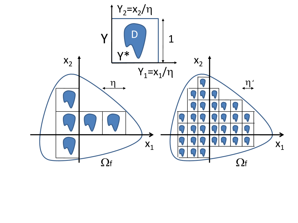
Figure 11.1: A diagram of the homogenization process: when the parameter $\eta$ gets smaller ($\eta<\eta^{\prime}$), the number of cells inside the fixed domain $\Omega_{f}$ becomes larger. When $\eta\ll 1$, $\Omega_{f}$ is filled with a large number of small cells, and can thus be considered as an effective (or homogenized) medium. Such a medium is usually described by anisotropic parameters depending upon the resolution of auxiliary (“unit cell”) problems set on the rescaled microcopic cell $Y$ which typically contains one inclusion $D$.

Let us consider a doubly periodic grating of pitch $\eta$ and finite extent such as shown in Fig.11.1. An interesting problem to look at is that of transverse electric (TE) modes— when the magnetic field has the form $(0,0,H)$— propagating within a micro-structured fiber with infinite conducting walls. Such an eigenvalue problem is known to have a discrete spectrum: we look for eigenfrequencies $\omega$ and associated eigenfields $H$ such that:

$$({\cal P}_{\eta}):\left\{\begin{array}[]{ll}\displaystyle{-\sum_{i,j=1}^{2}\frac{\partial}{\partial x_{i}}\left(\varepsilon_{ij}^{-1}(\frac{{\bf x}}{\eta})\frac{\partial H({\bf x})}{\partial x_{j}}\right)}=\omega^{2}\mu_{0}\varepsilon_{0}H({\bf x})&\hbox{in $\Omega_{f}$}\;,\\ \displaystyle{\varepsilon_{ij}^{-1}(\frac{{\bf x}}{\eta})\frac{\partial H({\bf x})}{\partial x_{i}}n_{j}}=0&\hbox{on $\partial\Omega_{f}$}\;,\end{array}\right.$$

where we use the convention ${\bf x}=(x_{1},x_{2})$, $\partial\Omega_{f}$ denotes the boundary $\Omega_{f}$, and ${\bf n}=(n_{1},n_{2})$ is the normal to the boundary. Here, $\varepsilon_{0}\mu_{0}=c^{-2}$ where $c$ is the speed of light in vacuum and we assume that matrix coefficients of relative permittivity $\varepsilon_{ij}({\bf y})$, with $i,j=1,2$, are real, symmetric (with the convention ${\bf y}=(y_{1},y_{2})$), of period $1$ (in $y_{1}$ et $y_{2}$) and satisfy:

$$M{\mid{\bm{\xi}}\mid}^{2}\geq\varepsilon_{ij}({\bf y})\xi_{i}\xi_{j}\geq m{\mid{\bm{\xi}}\mid}^{2}\;,\;\forall{\bm{\xi}}\in{\rm I\!R}^{2}\;,\;\forall{\bf y}\in Y={[0,1]}^{2}\;,$$ (11.1)

where ${\mid{\bm{\xi}}\mid}^{2}=(\xi_{1}^{2}+\xi_{2}^{2})$, for given strictly positive constants $M$ and $m$. This condition is met for all conventional dielectric media.

We can recast $({\cal P}_{\eta})$ as follows:

$$-\frac{\partial}{\partial x_{i}}\sigma^{i}(H({\bf x}))=\frac{\omega^{2}}{c^{2}}H({\bf x})$$

with

$$\sigma^{i}(H({\bf x}))=\varepsilon_{ij}^{-1}\left(\frac{{\bf x}}{\eta}\right)\frac{\partial H({\bf x})}{\partial x_{j}}\;.$$

The multiscale method relies upon the following ansatz:

$$H=H_{0}({\bf x})+\eta H_{1}({\bf x},{\bf y})+\eta^{2}H_{2}({\bf x},{\bf y})+...$$ (11.2)

where $H_{i}({\bf x},{\bf y})$, $i=1,2,...$ is a periodic function of period $Y$ in ${\bf y}$.

In order to proceed with the asymptotic algorithm, one needs to rescale the differential operator as follows

$$\frac{\partial H}{\partial x_{i}}=\left(\frac{\partial H_{0}}{\partial z_{i}}+\frac{\partial H_{1}}{\partial y_{i}}\right)+\eta\left(\frac{\partial H_{1}}{\partial z_{i}}+\frac{\partial H_{2}}{\partial y_{i}}\right)+...$$ (11.3)

where $\partial/\partial z_{i}$ stands for the partial derivative with respect to the $i$th component of the macroscopic variable ${\bf x}$.

It is useful to set

$$\sigma^{i}(H)=\sigma^{i}_{0}+\eta\sigma^{i}_{1}+\eta^{2}\sigma^{i}_{2}+...$$

what makes (11.3) more compact.

Collecting coefficients sitting in front of the same powers of $\eta$, we obtain:

$$\sigma^{i}_{0}(H)=\varepsilon_{ij}^{-1}({\bf y})\left(\frac{\partial H_{0}}{\partial z_{i}}+\frac{\partial H_{1}}{\partial y_{i}}\right)$$

$$\sigma^{i}_{1}(H)=\varepsilon_{ij}^{-1}({\bf y})\left(\frac{\partial H_{1}}{\partial z_{i}}+\frac{\partial H_{2}}{\partial y_{i}}\right)$$

and so forth, all terms being periodic in ${\bf y}$ of period $1$.

Upon inspection of problem $({\cal P}_{\eta})$, we gather that

$$-\left(\frac{1}{\eta}\frac{\partial}{\partial y_{i}}+\frac{\partial}{\partial z_{i}}\right)\left(\sigma^{i}_{0}+\eta\sigma^{i}_{1}+...\right)=\frac{\omega^{2}}{c^{2}}H({\bf x})+...$$

so that at order $\eta^{-1}$

$$({\cal A}):-\frac{\partial}{\partial y_{i}}\sigma^{i}_{0}=0\;,$$

and at order $\eta^{0}$

$$({\cal H}):-\frac{\partial}{\partial z_{i}}\sigma^{i}_{0}-\frac{\partial}{\partial y_{i}}\sigma^{i}_{1}=\frac{\omega^{2}}{c^{2}}H_{0}\;.$$

(the equations corresponding to higher orders in $\eta$ will not be used here).

Let us show that $({\cal H})$ provides us with an equation (known as the homogenized equation) associated with the macroscopic behaviour of the microstructured fiber. Its coefficients will be obtained thanks to $({\cal A})$ which is an auxiliary problem related to the microscopic scale. We will therefore be able to compute $H_{0}$ and $H_{1}$ thus, in particular, the first terms of $H$ and $\sigma^{i}$.

In order to do so, let us introduce the mean on $Y$, which we denote $<.>$, which is an operator acting on the function $g$ of the variable ${\bf y}$:

$$<g>=\frac{1}{\mid Y\mid}\int\int_{Y}g(y_{1},y_{2})dy_{1}dy_{2}\;,$$

where $\mid Y\mid$ is the area of the cell $Y$.

Applying the mean to both sides of $({\cal H})$, we obtain:

$$<({\cal H})>:-\frac{\partial}{\partial z_{i}}<\sigma^{i}_{0}>-<\frac{\partial}{\partial y_{i}}\sigma^{i}_{1}>=\frac{\omega^{2}}{c^{2}}H_{0}<1>\;,$$

where we have used the fact that $<.>$ commutes with $\partial/\partial z_{i}$.

Moreover, invoking the divergence theorem, we observe that

$$<\frac{\partial}{\partial y_{i}}\sigma^{i}_{1}>=\frac{1}{\mid Y\mid}\int\int_{Y}\frac{\partial}{\partial y_{i}}\sigma^{i}_{1}({\bf y})d{\bf y}=\frac{1}{\mid Y\mid}\int_{\partial Y}\sigma^{i}_{1}({\bf y})n_{i}ds\;,$$

where ${\bf n}=(n_{1},n_{2})$ is the unit outside normal to $\partial Y$ of $Y$. This normal takes opposite values on opposite sides of $Y$, hence the integral over $\partial Y$ vanishes.

Altogether, we obtain:

$$<({\cal H})>:-\frac{\partial}{\partial z_{i}}<\sigma^{i}_{0}>=\frac{\omega^{2}}{c^{2}}H_{0}\;,$$

which only involves the macroscopic variable $x$ and partial derivatives $\partial/\partial z_{i}$ with respect to the macroscopic variable. We now want to find a relation between $<\sigma_{0}>$ and the gradient in ${\bf x}$ of $H_{0}$. Indeed, we have seen that

$$\sigma^{i}_{0}(H)=\varepsilon_{ij}^{-1}({\bf y})\left(\frac{\partial H_{0}}{\partial z_{j}}+\frac{\partial H_{1}}{\partial y_{j}}\right)\;,$$

which from $({\cal A})$ leads to

$$({\cal A}1):-\frac{\partial}{\partial y_{i}}\left(\varepsilon_{ij}^{-1}({\bf y})\frac{\partial H_{1}}{\partial y_{j}}\right)=\left(\frac{\partial H_{0}}{\partial z_{j}}\right)\left(\frac{\partial}{\partial y_{i}}\varepsilon_{ij}^{-1}({\bf y})\right)\;.$$

We can look at $({\cal A}1)$ as an equation for the unknown $H_{1}({\bf x},{\bf y})$, periodic of period $Y$ in ${\bf y}$ and parametrized by ${\bf x}$. Such an equation is solved up to an additive constant. In addition to that, the parameter ${\bf x}$ is only involved via the factor $\partial H_{0}/\partial z_{j}$. Hence, by linearity, we can write the solution $H_{1}({\bf x},{\bf y})$ as follows:

$$H_{1}({\bf x},{\bf y})=\frac{\partial H_{0}({\bf x})}{\partial z_{j}}w^{j}({\bf y})\;,$$

where the two functions $w^{j}({\bf y})$, $j=1,2$ are solutions to $({\cal A}1)$ corresponding to $\partial H_{0}/\partial z_{j}({\bf x})$, $j=1,2$ equal to unity with the other ones being zero, that is solutions to:

$$({\cal A}2):-\frac{\partial}{\partial y_{i}}\left(\varepsilon_{ij}^{-1}({\bf y})\frac{\partial w^{k}}{\partial y_{j}}\right)=\delta_{jk}\left(\frac{\partial}{\partial y_{i}}\varepsilon_{ij}^{-1}({\bf y})\right)\;,$$

with $w^{k}({\bf y})$, $k=1,2$ periodic functions in ${\bf y}$ of period $Y$ .

Since the functions $w^{k}({\bf y})$ are known, we note that

$$\sigma_{i}^{0}({\bf x},{\bf y})=\varepsilon_{ij}^{-1}({\bf y})\left(\frac{\partial H_{0}}{\partial z_{j}}+\frac{\partial H_{1}}{\partial y_{j}}\right)=\varepsilon_{ij}^{-1}({\bf y})\left(\frac{\partial H_{0}}{\partial z_{j}}+\frac{\partial H_{0}}{\partial z_{k}}\frac{\partial w^{k}({\bf y})}{\partial y_{j}}\right)\;,$$

which can be written as

$$\sigma^{i}_{0}({\bf x},{\bf y})=\left(\varepsilon_{ik}^{-1}({\bf y})+\varepsilon_{ij}^{-1}({\bf y})\frac{\partial w^{k}({\bf y})}{\partial y_{j}}\right)\frac{\partial H_{0}({\bf x})}{\partial z_{k}}\;.$$

Lets us now apply the mean to both sides of this equation. We obtain:

$$<\sigma^{i}_{0}>({\bf x})=\varepsilon_{{\rm{hom}},ik}^{-1}\frac{\partial H_{0}({\bf x})}{\partial z_{k}}\;,$$

which can be recast as the following homogenized problem:

$$({\cal P}_{0}):\left\{\begin{array}[]{ll}\displaystyle{-\sum_{i,k=1}^{2}\frac{\partial}{\partial x_{i}}\left(\varepsilon_{{\rm{hom}},ik}^{-1}\frac{\partial H_{0}({\bf x})}{\partial x_{k}}\right)}=\omega^{2}\mu_{0}\varepsilon_{0}H_{0}({\bf x})&,\hbox{in $\Omega_{f}$}\;,\\ \displaystyle{\varepsilon_{{\rm{hom}},ik}^{-1}(\frac{{\bf x}}{\eta})\frac{\partial H_{0}({\bf x})}{\partial x_{i}}n_{k}}=0&,\hbox{on $\partial\Omega_{f}$}\;,\end{array}\right.$$

where $\varepsilon_{{\rm{hom}},ik}^{-1}$ denote the coefficients of the homogenized matrix of permittivity given by:

$$\varepsilon_{{\rm{hom}},ik}^{-1}=\frac{1}{\mid Y\mid}\int\int_{Y}\left(\varepsilon_{ik}^{-1}({\bf y})+\varepsilon_{ij}^{-1}({\bf y})\frac{\partial w^{k}({\bf y})}{\partial y_{j}}\right)\,d{\bf y}\;.$$ (11.4)

As an illustrative example for this homogenized problem, we consider a microstructured waveguide consisting of a medium with relative permittivity $\varepsilon=1.25$ with elliptic inclusions (of minor and major axes $0.3$ cm and $0.4$ cm respectively) with center to center spacing $d=0.1cm$ with an infinite conducting boundary i.e. Neumann boundary conditions in the TE polarization.

We use the COMSOL MULTIPHYSICS finite element package to solve the annex problem and we find that ${[\varepsilon_{\rm hom}]}$ from (11.4) writes as [26]

$$\left(\begin{array}[]{cc}1.9296204&-1.0533083\,10^{-16}\\ -44.417444\,10^{-18}&2.1127643\end{array}\right)\;,$$

with $<\varepsilon>_{Y}=2.2867255$. The off diagonal terms can be neglected.

If we assume that the transverse propagating modes in the metallic waveguide have a small propagation constant $\gamma\ll 1$, the above mathematical model describes accurately the physics. We show in Fig. 11.3 a comparison between two TE modes of the microstructured waveguide and its associated anisotropic homogenized counterpart. Both eigenfrequencies and eigenfields match well (note that we use the waveguide terminology wavenumber $k=\sqrt{\omega^{2}/c^{2}-\gamma^{2}}$).

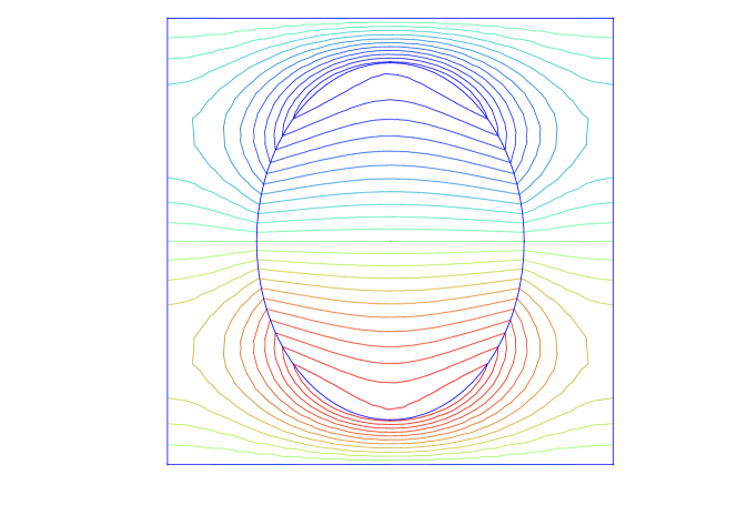
Figure 11.2: Potentials $V_{x}$ (left) and $V_{y}$ (right): The unit cell contains an elliptic inclusion of relative permittivity ($\varepsilon=4.0+3i$) with minor and major axis $a=0.3$ and $b=0.4$ in silica $(\varepsilon=1.25)$.

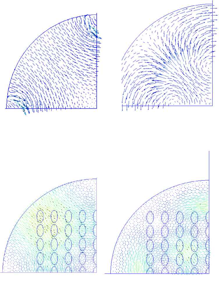
Figure 11.3: Comparison between transverse electric fields $TE_{21}$ and $TE_{31}$ of a microstructured metallic waveguide for a propagation constant $\gamma=0.1cm^{-1}$ (wavenumbers $k=0.7707cm^{-1}$ and $k=0.5478cm^{-1}$ respectively), see left panel, with the $TE_{21}$ and $TE_{31}$ modes of the corresponding homogenized anisotropic metallic waveguide for $\gamma=0.1cm^{-1}$ ($k=0.7607cm^{-1}$ and $k=0.5201cm^{-1}$, where $k=\sqrt{\omega^{2}/c^{2}-\gamma^{2}}=\sqrt{\omega^{2}\varepsilon_{0}\mu_{0}-\gamma^{2}}$ were obtained from the computation of eigenvalues $\omega$ of homogenized problem $({\cal P}_{0})$), see right panel.

11.1.3 The case of one-dimensional gratings: Application to invisibility cloaks

There is a case of particular importance for applications in grating theory: that of a periodic multilayered structure. Let us assume that the permittivity of this medium is $\varepsilon=\alpha$ in white layers and $\beta$ in yellow layers, as shown in Fig. 11.4.

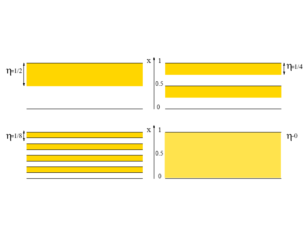
Figure 11.4: Schematic of homogenization process for a one-dimensional grating with homogeneous dielectric layers of permittivity $\alpha$ and $\beta$ in white and yellow regions. When $\eta$ tends to zero the number of layers tends to infinity, and their thicknesses vanish, in such a way that the width of the overall stack remains constant.

Equation $({\cal A}2)$ takes the form:

$$({\cal A}3):-\frac{d}{dy}\left(\varepsilon^{-1}({y})\frac{dw}{\partial y}\right)=\left(\frac{d}{dy}\varepsilon^{-1}({y})\right)\;,$$

with $w({y})$, periodic function in $y$ of period $1$.

We deduce that

$$-\frac{dw}{dy}=1+C\varepsilon({y})\;.$$

Noting that $\displaystyle{\int_{Y}\frac{dw}{dy}}=w(1)-w(0)=0$, this leads to

$$\int_{Y}\left(1+C\varepsilon({y})\right)dy=0\;.$$

Since $\mid Y\mid=1$, we conclude that

$$C=-{<\varepsilon>}^{-1}\;.$$

The homogenized permittivity takes the form:

$$\begin{array}[]{lll}\varepsilon_{{\rm hom}}^{-1}&=\displaystyle{\frac{1}{\mid Y\mid}\int_{Y}\left(\varepsilon^{-1}({y})+\varepsilon^{-1}({y})\frac{dw({y})}{dy}\right)\,dy}\\ &=<\varepsilon^{-1}({y})>-<\varepsilon^{-1}({y})+C>\\ &=<\varepsilon^{-1}({y})>-<\varepsilon^{-1}({y})>+<{<\varepsilon({y})>}^{-1}>={<\varepsilon({y})>}^{-1}\;.\end{array}$$

We note that if we now consider the full operator i.e. we include partial derivatives in $y_{1}$ and $y_{2}$, the anisotropic homogenized permittivity takes the form:

$$\varepsilon_{{\rm hom}}^{-1}=\left(\begin{array}[]{cc}{<\varepsilon({y})^{-1}>}&0\\ 0&{<\varepsilon({y})>}^{-1}\end{array}\right)\;,$$

as the only contribution for $\varepsilon_{{\rm hom},11}^{-1}$ is $1/\mid Y\mid\int_{Y}\varepsilon^{-1}(y)\,dy$.

As an illustrative example of what artificial anisotropy can achieve, we propose the design of an invisibility cloak. For this, let us assume that we have a multilayered grating with periodicity along the radial axis. In the coordinate system $(r,\theta)$, the homogenized permittivity clearly has the same form as above. If we want to design an invisibility cloak with an alternation of two homogeneous isotropic layers of thicknesses $d_{A}$ and $d_{B}$ and permittivities $\alpha$, $\beta$, we then need to use the formula

$$\begin{array}[]{lll}&\displaystyle{\frac{1}{\varepsilon_{r}}}=\displaystyle{\frac{1}{1+\eta}\left(\frac{1}{\alpha}+\frac{\eta}{\beta}\right)},&\varepsilon_{\theta}=\displaystyle{\frac{\alpha+\eta\beta}{1+\eta}}\;,\end{array}$$

where $\eta=d_{B}/d_{A}$ is the ratio of thicknesses for layers $A$ and $B$ and $d_{A}+d_{B}=1$.

We now note that the coordinate transformation $r^{\prime}=R_{1}+r\frac{R_{2}-R_{1}}{R_{2}}$ can compress a disc $r<R_{2}$ into a shell $R_{1}<r<R_{2}$, provided that the shell is described by the following anisotropic heterogeneous permittivity [27] $\underline{\underline{\varepsilon}}^{{\rm cloak}}$ (written in its diagonal basis):

$$\begin{array}[]{lll}\varepsilon_{r}^{{\rm cloak}}&=\displaystyle{{\left(\frac{R_{2}}{R_{2}-R_{1}}\right)}^{2}}{\left(\frac{r^{\prime}-R_{1}}{r^{\prime}}\right)}^{2}\;,&\varepsilon_{\theta}^{{\rm cloak}}=\displaystyle{{\left(\frac{R_{2}}{R_{2}-R_{1}}\right)}^{2}}\;,\end{array}$$ (11.5)

where $R_{1}$ and $R_{2}$ are the interior and the exterior radii of the cloak. Such a metamaterial can be approximated using the formula (11.1.3), as first proposed in [28], which leads to the multilayered cloak shown in Fig. 11.5.

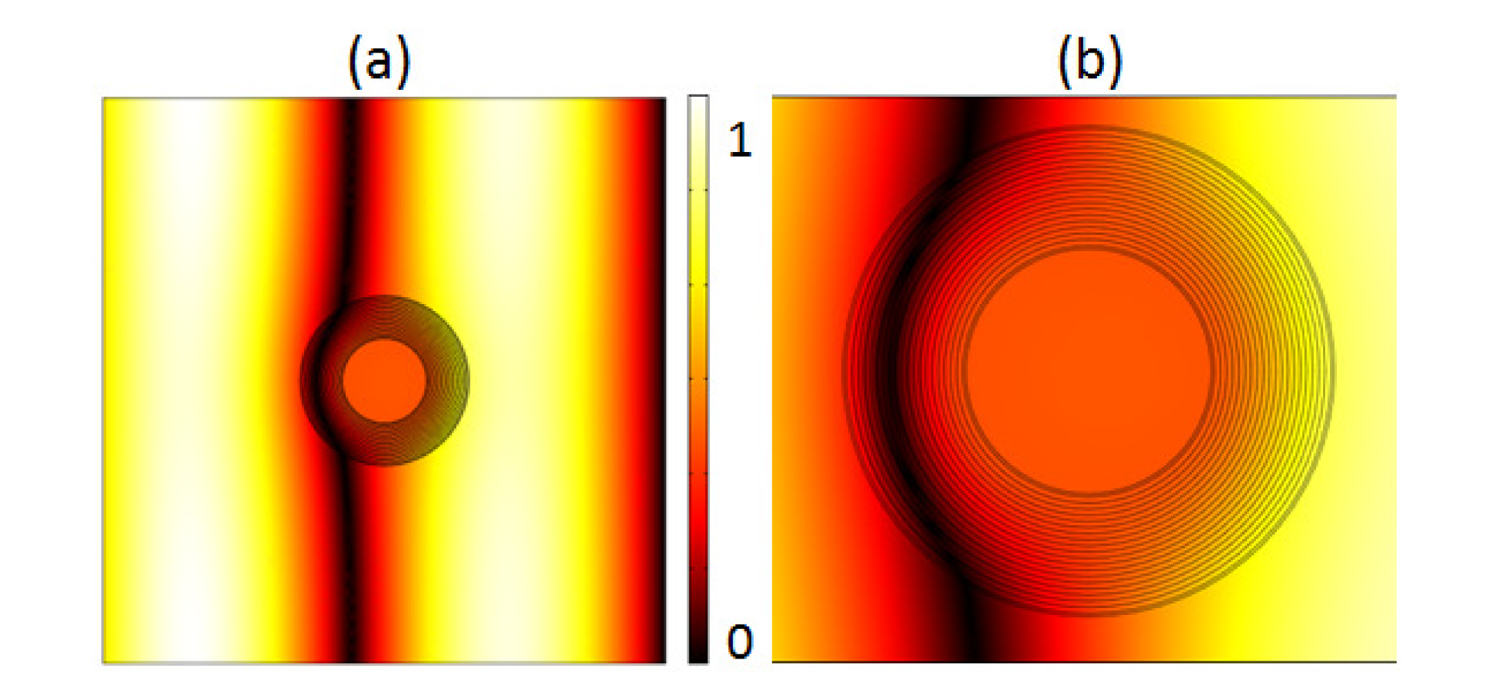
Figure 11.5: Propagation of a plane wave of wavelength $7\;10^{-7}$m (red in the visible spectrum) from the left on a multilayered cloak of inner radius $R_{1}=1.5\;10^{-8}$m and outer radius $R_{2}=3\;10^{-8}$m, consisting of 20 homogeneous layers of equal thickness and of respective relative permittivities $1680.70,0.25,80.75,0.25,29.39,0.25,16.37,0.25,10.99,0.25,8.18,0.25,6.50,0.25,5.40$, $0.25,4.63,0.25,4.06,0.25$ in vacuum. Importantly, one layer in two has the same permittivity.

11.2 High-frequency homogenization

Many of the features of interest in photonic crystals [44, 45], or other periodic structures, such as all-angle negative refraction [46, 47, 48, 49] or ultrarefraction [50, 51] occur at high frequencies where the wavelength and microstructure dimension are of similar orders. Therefore the conventional low-frequency classical homogenisation clearly fails to capture the essential physics and a different approach to distill the physics into an effective model is required. Fortunately a high frequency homogenisation (HFH) theory as developed in [37] is capable of capturing features such as AANR and ultra-refraction [52] for some model structures. Somewhat tangentially, there is an existing literature in the analysis community on Bloch homogenisation [53, 54, 55, 56], that is related to what we call high frequency homogenisation. There is also a flourishing literature on developing homogenised elastic media, with frequency dependent effective parameters, based upon periodic media [38]. There is therefore considerable interest in creating effective continuum models of microstructured media that break free from the conventional low frequency homogenisation limitations.

11.2.1 High Frequency Homogenization for Scalar Waves

Waves propagating through photonic crystals and metamaterials have proven to show different effects depending on their frequency. The homogenization of a periodic material is not unique. The effective properties of a periodic medium change depending on the vibration modes within its cells. The dispersion diagram structure can be considered to be the identity of such a material and provides the most important information regarding group velocities, band-gaps of dis-allowed propagation frequency bands, Dirac cones and many other interesting effects. The goal of a homogenization theory is to provide an effective homogeneous medium that is equivalent, in the long scale, to the initial non-homogeneous medium composed of a short-scale periodic, or other microscale, structure. This was achieved initially using the classical theory of homogenization [4, 34, 11, 35, 36] and yields an intuitively obvious result that the effective medium’s properties consist of simple averages of the original medium’s properties. This is valid so long as the wavelength is very large compared to the size of the cells (here we focus on periodic media created by repeating cells). For shorter wavelengths of the order of a cell’s length a more general theory has been developed [37] that also recovers the results of the classical homogenization theory. For clarity we present high frequency homogeniaztion (HFH) by means of an illustrative example and consider a two-dimensional lattice geometry for TE or TM polarised electromagnetic waves. With harmonic time dependence, $\exp(-i\Omega t)$ (assumed understood and henceforth suppressed), the governing equation is the scalar Helmholtz equation,

$$\nabla^{2}u+\Omega^{2}u=0,$$ (11.6)

where $u$ represent $E_{Z}$ and $H_{Z}$, for TM and TE polarised electromagnetic waves respectively, and $\Omega^{2}={n^{2}}\omega^{2}/{c^{2}}$. In our example the cells are square and each square cell of length $2l$ contains a circular hole and the filled part of the cell has constant non-dimensionalized properties. The boundary conditions on the hole’s surface, namely the boundary $\partial S_{2}$, depend on the polarisation and are taken to be either of Dirichlet or Neumann type. This approach assumes infinite conducting boundaries which is a good approximation for micro-waves. We adopt a multiscale approach where $l$ is the small length scale and $L$ is a large length scale and we set $\eta=l/L\ll 1$ to be the ratio of these scales. The two length scales let us introduce the following two independent spatial variables, $\xi_{i}=x_{i}/l$ and $X_{i}=x_{i}/L$. The cell’s reference coordinate system is then $-1<\xi<1$. By introducing the new variables in equation (11.6) we obtain,

$$u({\bf X},{\bm{\xi}}),_{\xi_{i}\xi_{i}}+\Omega^{2}u({\bf X},{\bm{\xi}})+2\eta u({\bf X},{\bm{\xi}}),_{\xi_{i}X_{i}}+\eta^{2}u({\bf X},{\bm{\xi}}),_{X_{i}X_{i}}=0.$$ (11.7)

We now pose an ansatz for the field and the frequency,

$$u({\bf X},{\bm{\xi}})=u_{0}({\bf X},{\bm{\xi}})+\eta u_{1}({\bf X},{\bm{\xi}})+\eta^{2}u_{2}({\bf X},{\bm{\xi}})+\ldots,$$

$$\Omega^{2}=\Omega_{0}^{2}+\eta\Omega_{1}^{2}+\eta^{2}\Omega_{2}^{2}+\ldots$$ (11.8)

In this expansion we set $\Omega_{0}$ to be the frequency of standing waves that occur in the perfectly periodic setting. By substituting equations (11.8) into equation (11.7) and grouping equal powers of $\epsilon$ through to second order, we obtain a hierarchy of three ordered equations:

$$u_{0,\xi_{i}\xi_{i}}+\Omega_{0}^{2}u_{0}=0,$$ (11.9)

$$u_{1,\xi_{i}\xi_{i}}+\Omega_{0}^{2}u_{1}=-2u_{0,\xi_{i}X_{i}}-\Omega_{1}^{2}u_{0},$$ (11.10)

$$u_{2,\xi_{i}\xi_{i}}+\Omega_{0}^{2}u_{2}=-u_{0,X_{i}X_{i}}-2u_{1,\xi_{i}X_{i}}-\Omega_{1}^{2}u_{1}-\Omega_{2}^{2}u_{0}.$$ (11.11)

These equations are solved as in [40, 37] and hence the description is brief.

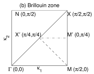
Figure 11.6: Panel (a) An infinite square array of split ring resonators with the elementary cell shown as the dashed line inner square. Panel (b) shows the irreducible Brillouin zone, in wavenumber space, used for square arrays in perfectly periodic media based around the elementary cell shown of length $2l$ ($l=1$ in (b)). Figure reproduced from Proceedings of the Royal Society [40].

The asymptotic expansions are taken about the standing wave frequencies that occur at the corners of the irreducible Brillouin zone depicted in Fig. 11.6. It should be noted that not all structured cells will have the usual symmetries of a square, as in Fig. 11.6(a) where there is no reflexion symmetry from the diagonals. As a consequence the usual triangular region $\Gamma XM$ does not always represent the irreducible Brillouin zone and the square region $\Gamma MXN$ should be used instead. Also paths that cross the irreducible Brillouin zone have proven to yield interesting effects namely along the path $MX^{\prime}$ for large circular holes [39].

The subsequent asymptotic development considers small perturbations about the points $\Gamma$, $X$ and $M$ so that the boundary conditions of $u$ on the outer boundaries of the cell, namely $\partial S_{1}$, read,

$$u|_{\xi_{i}=1}=\pm u|_{\xi_{i}=-1}\quad\text{and}\quad u_{,\xi_{i}}|_{\xi_{i}=1}=\pm u_{,\xi_{i}}|_{\xi_{i}=-1},$$ (11.12)

where the $+,-$ stand for periodic and anti-periodic conditions respectively: the standing waves occur when these conditions are met. The conditions on $\partial S_{2}$ are either of Dirichlet or Neumann type. The theory that follows is similar for both boundary condition cases, but the latter one is illustrated herein. Neumann boudary condition on the hole’s surface or equivalently electromagnetic waves in TE polarization yield,

$$\frac{\partial u}{\partial{\bf n}}=u_{,x_{i}}n_{i}|_{\partial S_{2}}=0.$$ (11.13)

which in terms of the two-scales and $u_{i}({\bf X},{\bm{\xi}})$ become

$$U_{0,\xi_{i}}n_{i}=0,\quad(U_{0}f_{0,X_{i}}+u_{1,\xi_{i}})n_{i}=0,\quad(u_{1,X_{i}}+u_{2,\xi_{i}})n_{i}=0.$$ (11.14)

The solution of the leading order equation is by introducing the following separation of variables $u_{0}=f_{0}({\bf X})U_{0}({\bm{\xi}};\Omega_{0})$. It is obvious that $f_{0}({\bf X})$, which represents the behaviour of the solution in the long scale, is not set by the leading order equation and the resulting eigenvalue problem is solved on the short-scale for $\Omega_{0}$ and $U_{0}$ representing the standing wave frequencies and the associated cell’s vibration modes respectively. To solve the first order equation (11.10) we take the integral over the cell of the product of equation (11.10) with $U_{0}$ minus the product of equation (11.9) with $u_{1}/f_{0}$ and this yields $\Omega_{1}=0$. It then follows to solve for $u_{1}({\bf X},{\bm{\xi}})=f_{0,X_{i}}({\bf X})U_{1_{i}}({\bm{\xi}})$ where the vector ${\bf U}_{1}$ is found as in [40]. By invoking a similar solvability condition for the second order equation we obtain a second order PDE for $f_{0}({\bf X})$,

$$T_{ij}f_{0,X_{i}X_{j}}+\Omega_{2}^{2}f_{0}=0\quad{\rm where},$$

$$\quad T_{ij}=\frac{t_{ij}}{\int\int_{S}U_{0}^{2}dS}\quad{\rm for}\quad i,j=1,2$$ (11.15)

entirely on the long scale with the coefficients $T_{ij}$ containing all the information of the cell’s dynamical response and the tensor $t_{ij}$ represents dynamical averages of the properties of the medium. For Neumann boundary conditions on $\partial S_{2}$ its formulation reads,

$$t_{ii}=\int\int_{S}U_{0}^{2}dS+\int\int_{S}(U_{1_{i},\xi_{i}}U_{0}-U_{1_{i}}U_{0,\xi_{i}})dS\quad{\rm for}\quad i=1\ {\rm or}\ 2,$$ (11.16)

$$t_{ij}=\int\int_{S}(U_{1_{j},\xi_{i}}U_{0}-U_{1_{j}}U_{0,\xi_{i}})dS\quad{\rm for}\quad i\neq j.$$ (11.17)

Note that there is no summation over repeated indexes for $t_{ii}$. The tensor depends on the boundary conditions of the holes and has a different form if Dirichlet type conditions are applied on $\partial S_{2}$.

The PDE for $f_{0}$ has several uses, and can be verified by re-creating asymptotically the dispersion curves for a perfect lattice system. One important result of equation (11.15) is its use in the expansion of $\Omega$ namely in equation (11.8). In order to obtain $\Omega_{2}$ as a function of the Bloch wavenumbers we use the Bloch boundary conditions on the cell to solve for $f_{0}({\bf X})=\exp(i\kappa_{j}X_{j}/\eta)$, where $\kappa_{j}=K_{j}-d_{j}$ with $d_{j}=0,\pi/2,-\pi/2$ depending on the location in the Brillouin zone. The asymptotic dispersion relation now reads,

$$\Omega\sim\Omega_{0}+\frac{T_{ij}}{2\Omega_{0}}\kappa_{i}\kappa_{j}.$$ (11.18)

Equation (11.18) yields the behaviour of the dispersion curves asymptotically around the standing wave frequencies that are naturally located at the edge points of the Brillouin zone. Fig. 11.8 illustrates the asymptotic dispersion curves for the first six dispersion bands of a square cell geometry with circular holes.

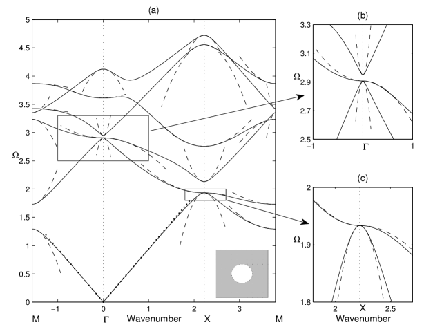
Figure 11.7: The dispersion diagram for a doubly periodic array of square cells with circular inclusions, of radius $0.4$, free at their inner boundaries shown for the irreducible Brillouin zone of Fig. 11.6. The dispersion curves are shown in solid lines and the asymptotic solutions from the high frequency homogenization theory are shown in dashed lines. Figure reproduced from Proceedings of the Royal Society [40].

An assumption in the development of equation (11.18) is that the standing wave frequencies are isolated. But one can clearly see in Fig. 11.7 that this is not the case for third standing wave frequency at point $\Gamma$ as well as for the second standing wave frequency at point $X$. A small alteration to the theory [40] enables the computation of the dispersion curves at such points by setting,

$$u_{0}=f_{0}^{(l)}({\bf X})U_{0}^{(l)}({\bm{\xi}};\Omega_{0})$$ (11.19)

where we sum over the repeated superscripts $(l)$. Proceeding as before, we multiply equation (11.10) by $U_{0}^{(m)}$, substract $u_{1}((U^{(m)}_{0,\xi_{i}})_{\xi_{i}}+\Omega_{0}^{2}U_{0}^{(m)})$ then integrate over the cell to obtain,

$$\left(\frac{\partial}{\partial X_{j}}{\bf A}_{jml}+\Omega_{1}^{2}{\bf B}_{ml}\right){\hat{f}}_{0}^{(l)}=0,\quad{\rm for}\quad m=1,2,\ldots,p$$ (11.20)

$\Omega_{1}$ is not necessarily zero, and

$${\bf A}_{jml}=\int\int_{S}(U_{0}^{(m)}U_{0,\xi_{j}}^{(l)}-U_{0,\xi_{j}}^{(m)}U_{0}^{(l)})dS,\quad{\bf B}_{ml}=\int\int U_{0}^{(l)}U_{0}^{(m)}dS.$$ (11.21)

There is now a system of coupled partial differential equations for the $f_{0}^{(l)}$ and, provided $\Omega_{1}\neq 0$, the leading order behaviour of the dispersion curves near the $\Omega_{0}$ is now linear (these then form Dirac cones).

For the perfect lattice, we set $f_{0}^{(l)}={\hat{f}}_{0}^{(l)}\exp(i\kappa_{j}X_{j}/\eta)$ and obtain the following index equations,

$$(i\frac{\kappa_{j}}{\eta}{\bf A}_{jml}+\Omega_{1}^{2}{\bf B}_{ml}){\hat{f}}_{0}^{(l)}=0,\quad\rm{for}\quad m=1,2,...,p$$ (11.22)

The system of equation (11.22) can be written simply as,

$${\bf C}{\hat{\bf F}}_{0}=0,$$ (11.23)

with ${\bf C}_{ll}=\Omega_{1}^{2}{\bf B}_{ll}$ and ${\bf C}_{ml}=i\kappa_{j}{\bf A}_{jml}/\eta$ for $l\neq m$. One must then solve for $\Omega_{1}^{2}=\pm\sqrt{\alpha_{ij}\kappa_{i}\kappa_{j}}/\eta$ when the determinant of ${\bf C}$ vanishes and insert the result in,

$$\Omega\sim\Omega_{0}\pm\frac{1}{2\Omega_{0}}\sqrt{\alpha_{ij}\kappa_{i}\kappa_{j}}.$$ (11.24)

If the $\Omega_{1}$ are zero one must go to the next order.

Repeated eigenvalues: quadratic asymptotics

If $\Omega_{1}$ is zero, $u_{1}=f_{0,X_{k}}^{(l)}U_{1_{k}}^{(l)}$ (we again sum over all repeated $(l)$ superscripts) and we advance to second order using (11.11). Taking the difference between the product of equation (11.11) with $U_{0}^{(m)}$ and $u_{2}(U_{0,\xi_{i}\xi_{i}}+\Omega_{0}^{2}U_{0})$ and then integrating over the elementary cell gives

$$f_{0,X_{i}X_{i}}^{(l)}\int\int_{S}U_{0}^{(m)}U_{0}^{(l)}dS+f_{0,X_{k}X_{j}}^{(l)}\int\int_{S}(U_{0}^{(m)}U_{1_{k},\xi_{j}}^{(l)}-U_{0,\xi_{j}}^{(m)}U_{1_{k}}^{(l)})dS$$

$$\quad+\Omega_{2}^{2}f_{0}^{(l)}\int\int_{S}U_{0}^{(m)}U_{0}^{(l)}dS=0,\quad{\rm for}\quad m=1,2,...,p$$ (11.25)

as a system of coupled PDEs. The above equation is presented more neatly as

$$f_{0,X_{i}X_{i}}^{(l)}{\bf A}_{ml}+f_{0,X_{k}X_{j}}^{(l)}{\bf D}_{kjml}+\Omega_{2}^{2}f_{0}{\bf B}_{ml}=0,\quad{\rm for}\quad m=1,2,...,p.$$ (11.26)

For the Bloch wave setting, using $f_{0}^{(l)}({\bf X})={\hat{f}}_{0}^{(l)}\exp(i\kappa_{j}X_{j}/\eta)$ we obtain the following system,

$$\left(-\frac{\kappa_{i}\kappa_{i}}{\eta^{2}}{\bf A}_{ml}-\frac{\kappa_{k}\kappa_{j}}{\eta^{2}}{\bf D}_{kjml}+\Omega_{2}^{2}{\bf B}_{ml}\right){\hat{f}}_{0}^{(l)}=0,\quad{\rm for}\quad m=1,2,...,p$$ (11.27)

and this determines the asymptotic dispersion curves.

The classical long wave zero frequency limit

The current theory simplifies if one enters the classical long wave, low frequency limit where $\Omega^{2}\sim O(\epsilon^{2})$ as $U_{0}$ becomes uniform, and without loss of generality is set to be unity, over the elementary cell. The final equation is again (11.15) where the tensor $t_{ij}$ simplifies to

$$t_{ii}=\int\int_{S}dS+\int\int_{S}U_{1_{i},\xi_{i}}dS,\quad t_{ij}=\int\int_{S}U_{1_{j},\xi_{i}}dS\quad{\rm for}\quad i\neq j$$ (11.28)

(with no summation over repeated suffices in this equation) and $T_{ij}=t_{ij}/\int\int_{S}dS$.

11.2.2 Illustrations for Tranverse Electric Polarized Waves

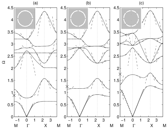
Figure 11.8: The dispersion diagrams for a doubly periodic array of square cells with split ring inclusions, free at their inner boundaries shown for the irreducible Brillouin zone of Fig. 11.6. The dispersion curves are shown in solid lines and the asymptotic solutions from the high frequency homogenization theory are shown in dashed lines. Figure reproduced from Proceedings of the Royal Society [40].

Let us now turn to some illustrative examples. We present in Fig. 11.8 the TE polarization waves for three types of SRR’s (Split Ring Resonator’s). Equation (11.15) represents the wave propagation in the effective medium. It is noticable that the $T_{ij}$ coefficients depend on the standing wave frequency and that $T_{11}$ is not necessarily equal to $T_{22}$ in order to yield an anisotropic effective medium for each separate frequency. Near some of the standing wave frequencies the anisotropy effects are very pronounced and well explained by the no longer elliptic equation (11.15).

In the above equations $U_{1_{i}}$ is a solution of,

$$U_{1_{j},\xi_{i}\xi_{i}}=0,$$ (11.29)

with boundary conditions $(f_{0,X_{i}}+u_{1,\xi_{i}})n_{i}=0$ on the hole boundary. If the medium is homogeneous as it is in the illustrative examples herein, equation (11.29) is the same as that for $U_{0}$, but with different boundary conditions. The specific boundary conditions for $U_{1_{j}}$ are

$$U_{1_{j},\xi_{i}}n_{i}=-n_{j}\quad\text{for}\quad j=1,2,$$ (11.30)

where $n_{i}$ represent the normal vector components to the hole’s surface. The role of ${\bf U_{1}}$ is to ensure Neumann boundary conditions hold and the tensor contains simple averages of inverse permittivity and permeability supplemented by the correction term which takes into account the boundary conditions at $\partial S_{2}$. Equation (11.28) is the classical expression for the homogenised coefficient in a scalar wave equation with constant material properties; (11.29) is the well-known annex problem of electrostatic type set on a periodic cell, see [4, 11], and also holds for the homogenised vector Maxwell’s system, where ${\bf U_{1}}$ now has three components and $i,j=1,2,3$ [41, 42, 43].

Cloaking in metamaterials

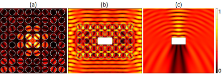
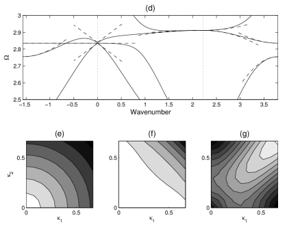
Figure 11.9: Cloaking in square arrays of SRRs with four holes: A source at frequency $\Omega=2.8$, located in the center of a square metamaterial consisting of 64 SRRs shaped as in Fig. 11.8(b) produces a wave pattern reminiscent of (a) concentric spherical field, (b) cloaking of a rectangular inclusion inside a slab of a metamaterial consisting of 38 SRRs and (c) scattering of a plane wave from the same rectangular hole as the previous panel. (d) Zoom in dispersion diagram of Fig. 11.8(b). Panels (e), (f) and (g) present isofrequency plots of the respective the lower, middle and upper modes of the Dirac point. Figure reproduced from Proceedings of the Royal Society [40].

SRRs with 4 holes are now used and the dispersion diagrams are in Fig. 11.8 (b). The flat band along the $M\Gamma$ path is interesting for the fifth mode and we choose to illustrate cloaking effects that occur here. In Fig. 11.9(a), we set an harmonic source at the corresponding frequency $\Omega=2.8$ in an $8\times 8$ array of SRRs and observe a wave pattern of concentric spherical modes. As can be seen in Figs. 11.9(b) and 11.9(c) a plane wave propagating at frequency $\Omega=2.8$ demonstrates perfect transmission through a slab composed of 38 SRRs but also cloaking of a rectangular inclusion where no scattering is seen before or after the metamaterial slab. Panel (d) of Fig. 11.9 shows the location in the band structure that is responsible for this effect. Note that the frequency of excitation is just below the Dirac cone point located at $\Omega=2.835$ where the group velocity is negative but also constant near that location of the Brillouin zone illustrated through an isofrequency plot of lower mode of the Dirac point in Fig. 11.9(e). In constrast with the isotropic features of panel (e), those of panels (f) and (g) show ultra-flattened isofrequency contours that relate to ultra-refraction, a regime more prone to omni-directivity than cloaking. The asymptotic system of equations (11.20) describing the effective medium at the Dirac point can be uncoupled to yield one same equation for all $f_{0}^{(j)}$’s,

$$f_{0,X_{i}X_{i}}^{(j)}+0.7191\Omega_{1}^{4}f_{0}^{(3)}=0$$ (11.31)

After some further analysis, the PDE for $f_{0}^{(2)}$ is responsible for the effects at the frequency chosen $\Omega=2.8$.

Lensing via AANR and St Andrew’s cross in metamaterials

We observe all-angle-negative-refraction effect in metamaterials with SRRs with 8 holes. The dispersion curves in Fig. 11.8(c) are interesting, as the second curve displays the hallmark of an optical band for a photonic crystal (it has a negative group velocity around the $\Gamma$ point). However, this band is the upper edge of a low frequency stop band induced by the resonance of a SRR, whereas the optical band of a PC results from multiple scattering, which thus arises at higher frequencies. We are therefore in presence of a periodic structure behaving somewhat as a composite intermediate between a metamaterial and a photonic crystal. One of the most topical subjects in photonics is the so-called all-angle-negative- refraction (AANR), which was first described in [46]. AANR allows one to focus light emitted by a point, onto an image, even through a flat lens, provided that certain conditions for AANR are met, such as convex isofrequency contours shrinking with frequency about a point in the Brillouin zone [49]. In Fig. 11.10, we show such an effect for a perfectly conducting photonic crystal (PC) in Fig. 11.10(a). In order to achieve AANR, we choose a frequency on the first dispersion curve (acoustic band) in Fig. 11.8(c), and we take its intersection with the light line $\Omega=\mid\kappa\mid$ along the $X\Gamma$ path. This means that we achieve negative group velocity for waves propagating along the $X\Gamma$ direction of the array, hence the rotation by an angle $\pi/4$ of every cell within the PC in panel (b) of Fig. 11.10. This is a standard trick in optics that has the effect of moving the origin of the light-line dispersion to $X$ as, relative to the PC, the Bloch wavenumber is along $X\Gamma$. This then creates optical effects due to the interaction of the light-line with the acoustic branch, this would be absent if $\Gamma$ were the light-line origin.

The anisotropy of the effective material is reflected from coefficients $T_{11}=-5.53$ and $T_{22}=0.2946$. The same frequency of the first band is reachable at point $N$ of the Brillouin zone. By symmetry of the crystal, we would have $T_{11}=0.2946$ and $T_{22}=-5.53$. The resultant propagating waves would come from the superposition of the two effective media described above. Fig. 11.10(b) illustrates this anisotropy as the source wave only propagates at the prescribed directions.

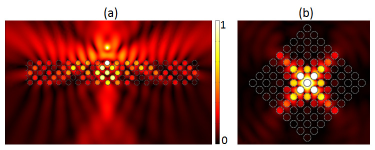
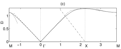
Figure 11.10: Lensing via AANR and St Andrew’s cross in square arrays of SRRs with eight holes: (a) A line source at frequency $\Omega=1.1375$ located above a rectangular metamaterial consisting of of 90 SRRs as in Fig. 11.8(c) displays an image underneath (lensing); (b) A line source at frequency $\Omega=1.25$ located inside a square metamaterial consisting of 49 SRRs as in Fig. 11.8(c) displays the dynamically induced anisotropy of the effective medium; (c) Zoom in dispersion diagram of Fig. 11.8(c). Note that each cell in the arrays in (a) and (b) has been rotated through an angle $\pi/4$. Figure reproduced from Proceedings of the Royal Society [40].

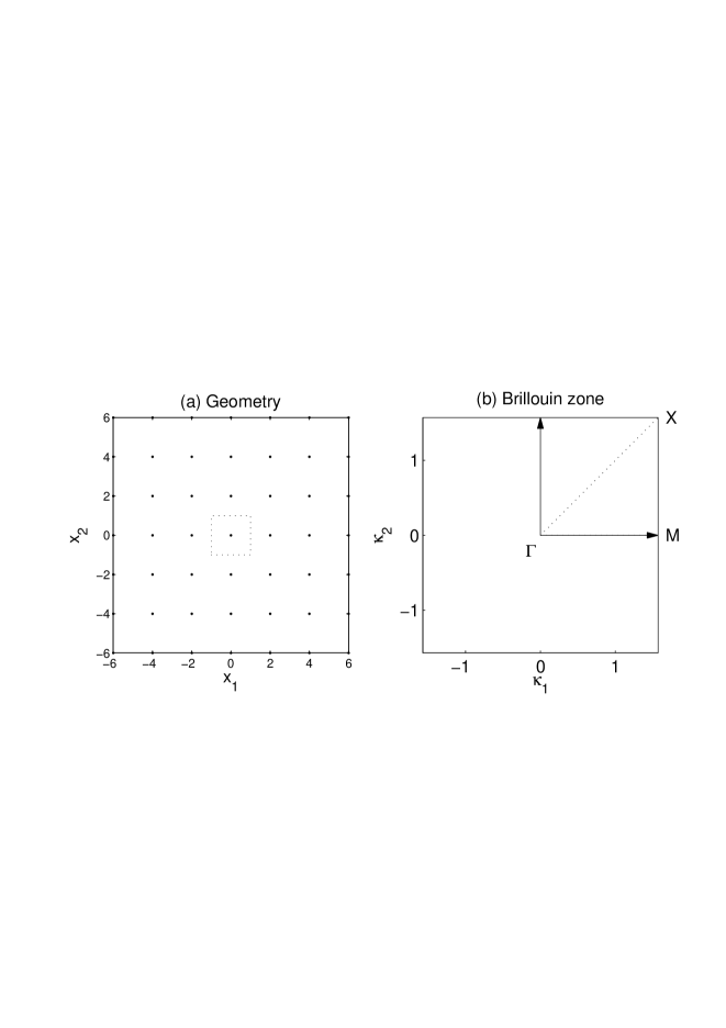
Figure 11.11: For the two dimensional example we show the geometry of the doubly periodic simply supported plate (the dots represent the simple supports) in panel (a) with the elementary cell shown by the dotted lines and in (b) the irreducible Brillouin zone with the lettering for wavenumber positions shown. Figure reproduced from Proceedings of the Royal Society [59].

11.2.3 Kirchoff Love Plates

HFH is by no means limited to the Helmholtz operator. HFH is here applied to flexural waves in two dimensions [59] for which the governing equation is a fourth order equation

$$\nabla^{4}u-\Omega^{2}u=0;$$ (11.32)

assuming constant material parameters. Such a thin plate can be subject to point, or line, constraints and these are common place in structural engineering.

In two dimensions, only a few examples of constrained plates are available in the literature: a grillage of line constraints as in [60] that is effectively two coupled one dimensional problems, a periodic line array of point supports [61] raises the possibility of Rayleigh-Bloch modes and for doubly periodic point supports there are exact solutions by [62] (simply supported points) and by [63] (clamped points); the simply supported case is accessible via Fourier series and we choose this as an illustrative example that is of interest in its own right; it is shown in figure 11.11(a). In particular the simply supported plate has a zero-frequency stop-band and a non-trivial dispersion diagram. It is worth noting that classical homogenization is of no use in this setting with a zero frequency stop band. Naturally waves passing through periodically constrained plates have many similarities with those of photonics in optics.

We consider a double periodic array of points at $x_{1}=2n_{1}$, $x_{2}=2n_{2}$ where $u=0$ (with the first and second derivatives continuous) and so the elementary cell is one in $|x_{1}|<1,|x_{2}|<1$ with $u=0$ at the origin (see Figure 11.11); Floquet-Bloch conditions are applied at the edges of the cell.

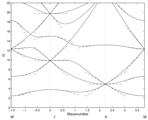
Figure 11.12: The dispersion diagram for a doubly periodic array of point simple supports shown for the irreducible Brillouin zone of Fig. 11.11. The figure shows the dispersion curves as solid lines. As dashed lines, the asymptotic solutions from the high frequency homogenization theory are shown. Figure reproduced from Proceedings of the Royal Society [59]

Applying Bloch’s theorem and Fourier series the displacement is readily found [62] as

$$u({\bf x})=\exp(i{\bm{\kappa}}\cdot{\bf x})\sum_{n_{1},n_{2}}\frac{\exp(-i\pi{\bf N}\cdot{\bf x})}{[(\kappa_{1}-\pi n_{1})^{2}+(\kappa_{2}-\pi n_{2})^{2}]^{2}-\Omega^{2}},$$ (11.33)

where ${\bf N}=(n_{1},n_{2})$, and enforcing the condition at the origin gives the dispersion relation

$$D(\kappa_{1},\kappa_{2},\Omega)=\sum_{n_{1},n_{2}}\frac{1}{[(\pi n_{1}-\kappa_{1})^{2}+(\pi n_{2}-\kappa_{2})^{2}]^{2}-\Omega^{2}}=0,$$ (11.34)

In this two dimensional example a Bloch wavenumber vector ${\bm{\kappa}}=(\kappa_{1},\kappa_{2})$ is used and the dispersion relation can be characterised completely by considering the irreducible Brillouin zone $\Gamma XM$ shown in figure 11.11.

The dispersion diagram is shown in figure 11.12; The singularities of the summand in equation (11.34) correspond to solutions within the cell satisfying the Bloch conditions at the edges, in some cases these singular solutions also satisfy the conditions at the support and are therefore true solutions to the problem, a similar situation occurs in the clamped case considered using multipoles in [63]. Solid lines in figure 11.12 label curves that are branches of the dispersion relation, notable features are the zero-frequency stop-band and also crossings of branches at the edges of the Brillouin zone. Branches of the dispersion relation that touch the edges of the Brillouin zone singly fall into two categories, those with multiple modes emerging at a same standing wave frequency (such as the lowest branch touching the left handside of the figure at M) and those that are completely alone (such as the second lowest branch on the left at M).

The HFH theory can again be employed to find an effective PDE entirely upon the long-scale that describes the behaviour local to the standing wave frequencies and the details are in [59], the asymptotics from the effective PDE are shown in Fig. 11.12 as the dashed lines.

11.3 High-contrast homogenization

Periodic media offer a convenient tool in achieving control of electromagnetic waves, due to their relative simplicity from the point of view of the manufacturing process, and due to the possibility of using the Floquet-Bloch decomposition for the analysis of the spectrum of the wave equation in such media. The latter issue has received a considerable amount of interest in the mathematical community, in particular from the perspective of the inverse problem: how to achieve a given spectrum and/or density of states for the wave operator with periodic coefficients by designing an appropriate periodic structure? While the Floquet-Bloch decomposition provides a transparent procedure for answering the direct question, it does not yield a straightforward way of addressing the inverse question posed above.

One possibility for circumventing the difficulties associated with the inverse problem is by viewing the given periodic structure as a high-contrast one, if this is possible under the values of the material parameters used. The idea of considering high-contrast composites within the context of homogenization appeared first in the work by Allaire [16], which discussed the application of the two-scale convergence technique (Nguetseng [8]) to classical homogenization. A more detailed analysis of high-contrast composites, along with the derivation of an explicit formula for the related spectrum, was carried out in a major study by Zhikov [18]. One of the obvious advantages in using high-contrast composites, or viewing a given composite as a high-contrast one, is in the mere existence of such formula for the spectrum. In the present section we focus on the results of the analysis of Zhikov, and on some more recent results for one-dimensional, layered, high-contrast periodic structures.

In order to get an as short as possible approach to the high-contrast theory, we consider the equation of electromagnetic wave propagation in the transverse electric (TE) polarisation, when the magnetic field has the form $(0,0,H),$ in the presence of sources with spatial density $f({\bf x}):$

$$-{\rm div}(\varepsilon^{\eta})^{-1}\left({\bf x}/\eta\right)\nabla H({\bf x})=\omega^{2}H({\bf x})+f({\bf x}),\ \ \ \ {\bf x}\in\Omega\subset{\mathbb{R}}^{2},$$ (11.35)

where we normalise the speed of light $c$ to 1 for simplicity, which amounts to taking $\varepsilon_{0}\mu_{0}=1$ in section 11.3, and where the magnetic permeability is assumed to be equal to unity throughout the medium (i.e. $\mu=\mu_{0}$), and the function $f({\bf x})$ is assumed to vanish outside some set that has positive distance to the boundary of $\Omega.$ The inverse dielectric permittivity tensor $(\varepsilon^{\eta})^{-1}({\bf y})$ is assumed in this section, for simplicity, to be a scalar, taking values $\eta^{\gamma}I$ and $I,$ respectively, on $[0,1]^{2}$-periodic open sets $F_{0}$ and $F_{1},$ such that $\overline{F_{0}}\cup\overline{F_{1}}={\mathbb{R}}^{2}.$ Here $\gamma$ is a positive exponent representing a “contrast” between material properties of the two components of the structure that occupy the regions $F_{0}$ and $F_{1}.$ In what follows we also assume that $F_{0}\cap[0,1]^{2}$ has a finite distance to the boundary of the unit cell $[0,1]^{2},$ so that the “soft” component $F_{0}$ consists of disjoint “inclusions”, spaced $[0,1]^{2}$-periodically from each other, while the “stiff” component $F_{1}$ is a connected subset of ${\mathbb{R}}^{2}.$ The matrix $\varepsilon^{\eta}$ represents the dielectric permittivity of the medium at a given point, however the analysis and conclusions of this section are equally applicable to acoustic wave propagation, which is the context we borrow the terms “soft” and “stiff” from. The assumed relation between the values of dielectric permittivity $\varepsilon^{\eta}$ (in acoustics, between the “stiffnesses” ) on the two components of the structure is close to the setting of what has been described as “arrow fibres” in the physics literature on electromagnetics, see e.g [64].

A simple dimensional analysis shows that if $\omega\sim 1$ then the soft inclusions are in resonance with the overall field if and only if $\gamma=2,$ which is the case we focus on henceforth.

The above equation (11.35) describes the wave profile for a TE-wave in the cylindrical domain $\Omega\times{\mathbb{R}}$ domain, and it is therefore supplied with the Neumann condition $\partial H/\partial n=0$ on the boundary of the domain and with the Sommerfeld radiation condition $\partial H/\partial|x|-{\rm i}\omega H=o(|x|^{-1})$ as $|x|\to\infty.$

In line with the previous sections, we apply the method of two-scale asymptotic expansions to the above problem, seeking the solution $H=H(x_{1},x_{2})=H({\bf x})$ in the form (see also (11.2 in Section 11.1.2)

$$H({\bf x})=H_{0}({\bf x},{\bf x}/\eta)+\eta H_{1}({\bf x},{\bf x}/\eta)+\eta^{2}H_{2}({\bf x},{\bf x}/\eta)+...,$$ (11.36)

where the functions involved are $[0,1]^{2}$-periodic with respect to the “fast” variable $y=x/\eta.$ Substituting the expansion (11.36) into the equation (11.35) and rearranging the terms in the resulting expression in such a way that terms with equal powers of $\eta$ are grouped together, we obtain a sequence of recurrence relations for the functions $H_{k},$ $k=0,1,...,$ from which they are obtained sequentially. The first three of these equations can be transformed to the following system of equations for the leading-order term $H^{(0)}({\bf x},{\bf y})=u({\bf x})+v({\bf x},{\bf y}),$ ${\bf x}\in\Omega,$ ${\bf y}\in[0,1]^{2}:$

$$-{\rm div}\varepsilon_{\rm hom}^{-1}\nabla u({\bf x})=\omega^{2}\biggl{(}u({\bf x})+\int_{F_{0}\cap[0,1]^{2}}v({\bf x},{\bf y})d{\bf y}\biggr{)}+f({\bf x}),\ \ \ {\bf x}\in\Omega,$$ (11.37)

$$-\Delta_{\bf y}v({\bf x},{\bf y})=\omega^{2}\bigl{(}u({\bf x})+v({\bf x},{\bf y})\bigr{)}+f({\bf x}),\ \ \ \ y\in F_{0}\cap[0,1]^{2},\ \ \ \ v({\bf x},{\bf y})=0,\ \ \ y\in{F_{1}}\cap[0,1]^{2}.$$ (11.38)

These equations are supplemented by the boundary conditions for the function $u,$ of the same kind as in the problems with finite $\eta.$ For the sake of simplifying the analysis, we assume that those inclusions that overlap with the boundary of $\Omega$ are substituted by the “main”, “stiff” material, where $(\varepsilon^{\eta})^{-1}=I.$

In the equation (11.37), the matrix $\varepsilon_{\rm hom}$ is the classical homogenization matrix for the perforated medium $\varepsilon F_{1},$ see Section above. However, the properties of the system (11.37)–(11.38) are rather different to those for the perforated-medium homogenised limit, described by the equation $-{\rm div}\varepsilon_{\rm hom}^{-1}\nabla u({\bf x})=\omega^{2}u({\bf x})+f({\bf x}).$ As we shall see next, the two-scale structure of (11.37)–(11.38) means that the description of the spectra of the problems (11.35) in the limit as $\eta\to 0$ diverges dramatically from the usual moderate-contrast scenario.

The true value of the above limiting procedure is revealed by the statement of the convergence, as $\eta\to 0,$ of the spectra of the original problems to the spectrum of the limit problem described above, see [18] and by observing that the spectrum of the system (11.37)–(11.37) is evaluated easily as follows. We write an eigenfunction expansion for $v({\bf x},{\bf y})$ as a function of $y\in{F_{0}}\cap[0,1]^{2}:$

$$v({\bf x},{\bf y})=\sum_{k=0}^{\infty}c_{k}({\bf x})\psi_{k}({\bf y}),$$ (11.39)

where $\psi_{k}$ are the (real-valued) eigenfunctions of the Dirichlet problem $-\Delta\psi_{k}=\lambda_{k}\psi_{k},$ $y\in{F_{1}}\cap[0,1]^{2},$ arranged in the order of increasing eigenvalues $\lambda_{k},$ $k=0,1,...$ and orthonormalised according to the conditions $\int_{{F_{0}}\cap[0,1]^{2}}|\psi_{k}({\bf y})|^{2}d{\bf y}=1,$ $k=0,1,...,$ and $\int_{{F_{0}}\cap[0,1]^{2}}\psi_{k}({\bf y})\psi_{l}({\bf y})d{\bf y}=0,$ $k\neq l,$ $k,l=0,1,...$ Substituting (11.39) into (11.38), we find the values for the coefficients $c_{k},$ which yield an explicit expression for $v({\bf x},{\bf y})$ in terms of the function $u({\bf x}):$

$$v({\bf x},{\bf y})=\bigl{(}\omega^{2}u({\bf x})+f({\bf x})\bigr{)}\sum_{k=0}^{\infty}\Bigl{(}\int_{{F_{0}}\cap[0,1]^{2}}\psi_{k}({\bf y})d{\bf y}\Bigr{)}(\lambda_{k}-\omega^{2})^{-1}\psi_{k}({\bf y}).$$

Finally, using the last expression in the first equation in (11.37) yields an equation for the function $u$ only:

$$-{\rm div}\varepsilon_{\rm hom}^{-1}\nabla u({\bf x})=\beta(\omega^{2})\bigl{(}u({\bf x})+\omega^{-2}f({\bf x})),\ \ \ {\bf x}\in\Omega,$$ (11.40)

where the function $\beta,$ which first appeared in the work [18], is given by

$$\beta(\omega^{2})=\omega^{2}\biggl{(}1+\omega^{2}\sum_{k=0}^{\infty}\Bigl{(}\int_{{F_{0}}\cap[0,1]^{2}}\psi_{k}({\bf y})d{\bf y}\Bigr{)}^{2}(\lambda_{k}-\omega^{2})^{-1}\biggr{)}.$$ (11.41)

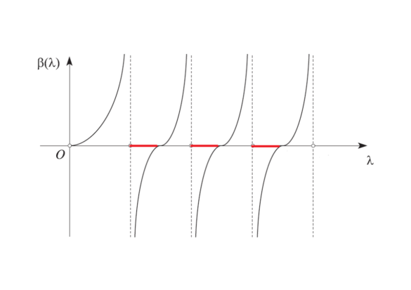
Figure 11.13: The plot of the function $\beta$ describing the spectrum of the problem (11.37)–(11.38) subject to the boundary conditions. The stop bands for the problem in the whole space ${\mathbb{R}}^{2}$ are indicated by the red intervals of the horizontal axis. The spectra of the problems (11.35) considered in the whole space converge, as $\eta\to 0,$ to the closure of the complement of the union of the red intervals in the positive semiaxis.

The equation (11.40) is supplemented by appropriate boundary conditions and/or conditions at infinity, which are inherited from the $\eta$-dependent family, i.e. the Neumann condition at the boundary points ${\bf x}\in\partial\Omega$ and the radiation condition when $|{\bf x}|\to\infty.$ Clearly, the spectrum of this limit problem consists of those values of $\omega^{2}$ for which $\beta(\omega^{2})$ is in the spectrum of the operator generated by the differential expression $-{\rm div}\varepsilon_{\rm hom}^{-1}\nabla$ subject to the same boundary conditions. For example, for the problem in the whole space ${\mathbb{R}}^{2}$ (describing the behaviour of TE-waves in a 3D periodic structure that is invariant in one specified direction) this procedure results in a band-gap spectrum shown in Fig. 11.13. The end points of each pass band are found by a simple analysis of the formula (11.41): the right ends of each pass band are given by those eigenvalues $\lambda_{k}$ of the Dirichlet Laplacian on the inclusion ${F_{0}}\cap[0,1]^{2}$ that possess at least one eigenfunction with non-zero integral over ${F_{0}}\cap[0,1]^{2}$ (otherwise the corresponding term in (11.41) vanishes), while the left ends of the pass bands are given by solutions to the polynomial equation of infinite order $\beta(\omega^{2})=0.$ These points have a physical interpretation as eigenvalues of the so-called electrostatic problem on the inclusion, see [23].

As in the case of classical, moderate-contrast, periodic media, the fact of spectral convergence offers significant computational advantages over tackling the equations (11.35) directly: as $\eta\to 0$ the latter becomes increasingly demanding, while the former requires a single numerical procedure that serves all $\eta$ once the homogenised matrix $\varepsilon_{\hom}$ and several eigenvalues $\lambda_{k}$ are calculated. A significant new feature, however, as compared to the classical case, is the fact of an infinite set of stop bands opening in the limit as $\eta\to,$ which are easily controlled by the explicit description of the band endpoints. This immediately yields a host of applications of the above results for the design of band-gap devices with prescribed behaviour in the frequency interval of interest.

The theorem on spectral convergence for problems described by the equation (11.35) is proved in [18] under the assumption of connectedness of the domain $F_{1}$ occupied by the “stiff” component, via a variant of the extension procedure from $F_{1}$ to the whole of ${\mathbb{R}}^{2}$ for function sequences whose energy scales as $\eta^{-2}$ (or, equivalently, finite-energy sequences for the operator prior to the rescaling ${\bf x}/\eta={\bf y}$). In the more recent works [24], [25], this assumption is dropped in a theorem about spectral convergence for a general class of high-contrast operators, via a version of the two-scale asymptotic analysis akin to (11.36), for the Floquet-Bloch components of the resolvent of the original family of operators following the re-scaling ${\bf x}/\eta={\bf y}.$ In particular, in [24] a one-dimensional high-contrast model is analysed, which in 3D corresponds to a stack of dielectric layers aligned perpendicular to the direction of the magnetic field. Here the procedure described above for the 2D grating fails to yield a satisfactory limit description as $\eta\to 0,$ i.e. a description where the spectra of problems for finite $\eta$ converge to the spectrum of the limit problem described by the system (11.37)–(11.38) as $\eta\to 0.$ A more refined analysis of the structure of the related $\eta$-dependent family results in a statement of convergence to the set described by the inequalities

$$-1\leq\frac{1}{2}(\alpha-\beta+1)\sqrt{\lambda}\sin\Bigl{(}\sqrt{\lambda}(\alpha-\beta)\Bigr{)}+\cos\Bigl{(}\sqrt{\lambda}(\alpha-\beta)\Bigr{)}\leq 1.$$ (11.42)

where $\alpha$ and $\beta$ denote the end-points of the inclusion in the unit cell, i.e. $F_{0}\cap[0,1]^{2}=(\alpha,\beta)\times[0,1].$

Similarly to the spectrum of the 2D high-contrast problem, described by the function $\beta,$ the limit spectrum of the 1D problem has a band-gap structure, shown in Fig. 11.14, however the description of the location of the bands is different in that it is no longer obtained from the inequality $\beta>0,$ where $\beta$ is the 1D analogue of (11.41). Importantly, the asymptotic behaviour of the density of states function as $\eta\to 0$ is also very different in the two cases. One can show that the family of resolvents for the problems (11.35) converges, up to a suitable unitary transformation, to the resolvent of a certain operator whose spectrum is given exactly by (11.42), see [25]. The rate of convergence is rigorously shown to be $O(\eta),$ as is anticipated by the expansion (11.36).

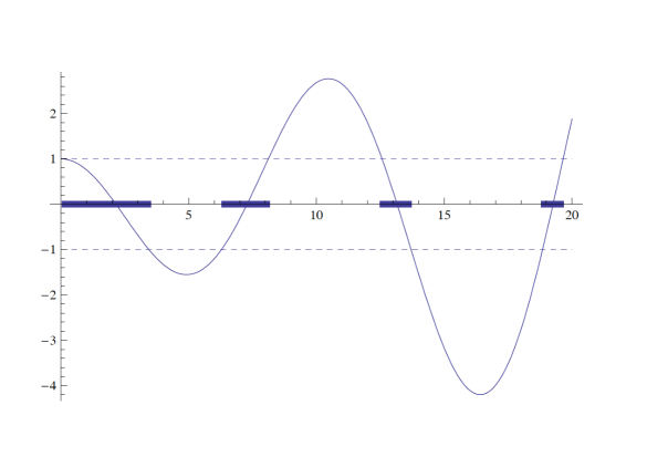
Figure 11.14: The square root of the limit spectrum for a 1D high-contrast periodic stack, in TE polarisation. The oscillating solid line is the graph of the function $f(\omega)=\cos(\omega/2)-\omega\sin(\omega/2)/4$ in (11.42) with $\alpha=1/4,$ $\beta=3/4.$ The square root of the spectrum is the union of the intervals indicated by bold lines.

The above 1D result is generalised to the case of an oblique incidence of an electromagnetic wave on the same 3D layered structure. Suppose that $x_{2}$ is the coordinate across the stack. Then, assuming for simplicity that the wave vector $(\varkappa,0,0)$ is parallel to the direction $x_{1},$ it can be shown that all three components of the magnetic field are non-vanishing, with the magnetic component $H=H_{3}$ satisfying the equation

$$-\Bigl{(}(\varepsilon^{\eta})^{-1}(x/\eta)H^{\prime}(x)\Bigr{)}^{\prime}=\Bigl{(}\omega^{2}-(\varepsilon^{\eta})^{-1}(x/\eta)\varkappa^{2}\Bigr{)}H(x),$$

subject to the same boundary conditions as before. The modified limit spectrum for this family is given by those $\omega^{2}$ for which (cf. (11.42))

$$-1\leq\frac{1}{2}(\alpha-\beta+1)\biggl{(}\omega-\frac{\varkappa^{2}}{\omega}\biggr{)}\sin\Bigl{(}\sqrt{\lambda}(\alpha-\beta)\Bigr{)}+\cos\Bigl{(}\sqrt{\lambda}(\alpha-\beta)\Bigr{)}\leq 1,\ \ \ \ \omega>0,$$ (11.43)

where, as before, $\alpha$ and $\beta$ describe the “soft" inclusion layer in the unit cell, see [24]. The set of $\omega$ described by the inequalities (11.43) is similar to that shown in Figure 11.14, the only significant difference between the two cases being a low-frequency gap opening near $\omega=0$ for (11.43).

11.4 Conclusion and further applications of grating theory

To conclude this chapter, we would like to stress that advances in homogenization theory over the past forty years have been fuelled by research in composites [36]. The philosophy of the necessity for rigour expressed by Lord Rayleigh in 1892 concerning the Lorentz-Lorenz equations (also known as Maxwell-Garnett formulae) can be viewed as the foundation act of homogenization: ‘In the application of our results to the electric theory of light we contemplate a medium interrupted by spherical, or cylindrical, obstacles, whose inductive capacity is different from that of the undisturbed medium. On the other hand, the magnetic constant is supposed to retain its value unbroken. This being so, the kinetic energy of the electric currents for the same total flux is the same as if there were no obstacles, at least if we regard the wavelength as infinitely great.’ In this paper, John William Strutt, the third Lord Rayleigh [29], was able to solve Laplace’s equation in two dimensions for rectangular arrays of cylinders, and in three-dimensions for cubic lattices of spheres. The original proof of Lord Rayleigh suffered from a conditionally convergent sum in order to compute the dipolar field in the array. Many authors in the theoretical physics and applied mathematics communities proposed extensions of Rayleigh’s method to avoid this drawback. Another limit of Rayleigh’s algorithm is that it does not hold when the volume fraction of inclusions increases. So-called multipole methods have been developed in conjunction with lattice sums in order to overcome such obstacles, see e.g. [30] for a comprehensive review of these methods. In parallel to these developments, the quasi-static limit for gratings has been the subject of intensive research, one might cite [31] and [32] for important contributions in the 1980s, and [33] for a comprehensive review of the modern theory of gratings, including a close inspection of homogenization limit.

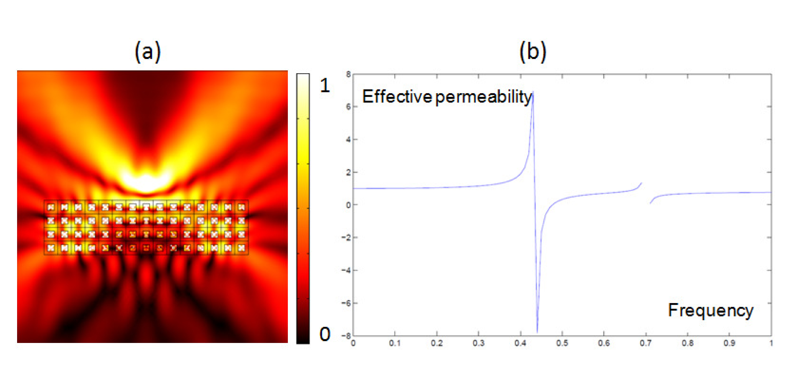
Figure 11.15: Superlens application of grating: (a) A time harmonic source at frequency $0.473$ displays an image through a square array of square inclusions; (b) Effective magnetism versus frequency using (11.44) for square inclusions of relative permittivity $100$ with sidelength $a=0.5d$ in matrix of relative permittivity $1$ (grating pitch $d=0.1$); Negative values of the effective magnetism are in the frequency region $[0.432,0.534]$.

Interestingly, in the pure mathematics community, Zhikov’s work on high-contrast homogenization [18] has had important applications in metamaterials, with the interpretation of his homogenized equations in terms of effective magnetism first put forward by O’Brien and Pendry [65], and then by Bouchitté and Felbacq [66], although these authors did not seem to be aware at that time of Zhikov’s seminal paper [18]. In order to grasp the physical importance of (11.40)-(11.41), we consider the case of square inclusions of sidelength $a=d/2$, where $d$ is the pitch of a bi-periodic grating. The eigenfunctions are $\psi_{nm}({\bf y})=2\sin(n\pi y_{1})\sin(n\pi y_{2})$ in (11.41) and the corresponding eigenvalues are $k^{2}_{nm}=\pi^{2}(n^{2}+m^{2})$. The right-hand side in the homogenized equation (11.40) can then be interpreted in terms of effective magnetism:

$$\mu_{hom}(k)=1+\frac{64a^{2}}{\pi^{4}}\sum_{(n,m)odd}\frac{k^{2}}{n^{2}m^{2}(k^{2}_{nm}/a^{2}-k^{2})}\;.$$ (11.44)

This function can be computed numerically for instance with Matlab and demonstrates that negative values can be achieved for $\mu_{hom}$ near resonances, see Fig. 11.15(b). This allows for superlensing via negative refraction, as shown in Fig. 11.15(a).

Finally, we would like to point out that high-order homogenization techniques [67] suggest that most gratings display some artificial magnetism and chirality when the wavelength is no longer much larger than the periodicity [68]. We hope we have convinced the reader that there is a whole new range of physical effects in gratings which classical, high-frequency and high-contrast homogenization theories can capture.

References:

- [1] Petit, R., 1980. Electromagnetic theory of gratings, Topics in current physics, Springer- Verlag, Berlin.
- [2] Bakhvalov, N. S.,1975. Averaging of partial differential equations with rapidly oscillating coefficients. Dokl. Akad. Nauk SSSR 221, 516–519. English translation in Soviet Math. Dokl. 16, 1975.
- [3] De Giorgi, E., Spagnolo, S., 1973. Sulla convergenza degli integrali dell’energia per operatori ellitici del secondo ordine. Boll. Unione Mat. Ital., Ser 8, 391–411.
- [4] Bensoussan, A., Lions, J.L., Papanicolaou, G., 1978. Asymptotic analysis for periodic structures, North-Holland, Amsterdam
- [5] Marchenko, V. A., Khruslov, E. Ja., 1964. Boundary-value problems with fine-grained boundary. (Russian) Mat. Sb. (N.S.) 65 (107) 458–472.
- [6] Tartar, L., 1974. Problème de côntrole des coefficients dans des équations aux dérivées partielles. Lecture Notes in Economics and Mathematical Systems 107, 420–426.
- [7] Murat, F., 1978. Compacité par compensation. (French) Ann. Scuola Norm. Sup. Pisa Cl. Sci. (4) 5(3), 489–507.
- [8] Nguetseng, G., 1989. A general convergence result for a functional related to the theory of homogenization. SIAM J. Math. Anal. 20 (3), 608–623.
- [9] Cioranescu, D., Damlamian, A., Griso, G., 2002. Periodic unfolding and homogenization, C. R. Math. Acad. Sci. Paris, 335, 99-104.
- [10] Bakhvalov, N. S., Panasenko, G. P., 1984. Homogenization: Averaging Processes in Periodic Media. Nauka, Moscow (in Russian). English translation in: Mathematics and its Applications (Soviet Series) 36, Kluwer Academic Publishers.
- [11] Jikov, V. V., Kozlov, S. M., Oleinik, O. A., 1994. Homogenization of Differential Operators and Integral Functionals. Springer, Berlin.
- [12] Sanchez-Palencia, E., 1980 Nonhomogeneous media and Vibration Theory. Lecture Notes in Physics 127, Springer, Berlin.
- [13] Chechkin, G. A., Piatnitski, A. L., Shamaev, A. S., 2007. Homogenization: Methods and Applications. AMS Translations of Mathematical Monographs 234.
- [14] Kozlov, S. M., 1979. The averaging of random operators. Mat. Sb. (N.S.), 109(151)(2),188–202.
- [15] Papanicolaou, G. C., Varadhan, S. R. S., 1981. Boundary value problems with rapidly oscillating random coefficients. Random fields, Vol. I, II (Esztergom, 1979), 835–873, Colloq. Math. Soc. János Bolyai, 27, North-Holland, Amsterdam-New York.
- [16] Allaire, G., 1992. Homogenization and two-scale convergence, SIAM J. Math. Anal. 23, 1482–1518.
- [17] Arbogast, T., Douglas, J., Hornung, U., 1990. Derivation of the double porosity model of single phase flow via homogenization theory. SIAM J. Math. Anal. 21 (4), 823-836.
- [18] Zhikov, V. V., 2000. On an extension of the method of two-scale convergence and its applications, Sb. Math., 191(7), 973–1014.
- [19] Kozlov, V., Mazya, V., Movchan, A., 1999. Asymptotic Analysis of Fields in Multi-structures, Oxford University Press, Oxford.
- [20] Mazya, V. G., Nazarov, S.A., Plamenevskii, B. A., 2000. Asymptotic Theory of Elliptic Boundary Value Problems in Singularly Perturbed Domains. Vol. I, Operator Theory: Advances and Applications 111, Birkäuser Verlag, Berlin.
- [21] Zhikov, V. V. , 2002. Averaging of problems in the theory of elasticity on singular structures. (Russian) Izv. Ross. Akad. Nauk Ser. Mat. 66 (2), 81–148. English translation in Izv. Math. 66 (2002), No. 2, 299–365.
- [22] Zhikov, V. V., Pastukhova, S. E., 2002. Averaging of problems in the theory of elasticity on periodic grids of critical thickness. (Russian) Dokl. Akad. Nauk 385 (5), 590–595.
- [23] Zhikov, V. V., 2005. On spectrum gaps of some divergent elliptic operators with periodic coefficients. St. Petersburg Math. J. 16(5) (2005), 774–790.
- [24] Cherednichenko. K. D., Cooper, S., Guenneau, S., 2012. Spectral analysis of one-dimensional high-contrast elliptic problems with periodic coefficients, Submitted.
- [25] Cherednichenko, K. D., Cooper, S., 2012. On the resolvent convergence of periodic differential operators with high contrast coefficients, Preprint.
- [26] Zolla, F., Guenneau, S., 2003. Artificial ferro-magnetic anisotropy : homogenization of 3D finite photonic crystals, in Movchan Ed. Asymptotics, singularities and homogenization in problems of mechanics, Kluwer Academic Press, 375–385.
- [27] Pendry, J.B., Schurig, D., Smith, D.R., 2006. Controlling Electromagnetic Fields, Science 312, 1780-1782.
- [28] Huang, Y., Feng, Y., Jiang, T., 2007. Electromagnetic cloaking by layered structure of homogeneous isotropic materials, Optics Express 15(18), 11133-11141.
- [29] Strutt, J.W. (Lord Rayleigh) 1892. On the influence of obstacles arranged in rectangular order upon the properties of a medium, Phil. Mag 34, 481-502.
- [30] Movchan, A.B., Movchan, N.V., Poulton, C.G., 2002. Asymptotic models of fields in dilute and densely packed composites, Imperial College Press, London.
- [31] McPhedran, R.C., Botten, L.C., Craig, M.S., Neviere, M., Maystre, D., 1982. Lossy Lamelar gratings in the quasistatic limit, Optica Acta 29, 289-312.
- [32] Petit, R., Bouchitte, G., 1987. Replacement of a very fine grating by a stratified layer: homogenisation techniques and the multiple-scale method, SPIE Proceedings, Application and Theory of Periodic Structures, Diffraction Gratings, and Moiré Phenomena 431, 815.
- [33] Neviere, M., Popov, E., 2003. Light Propagation in Periodic Media: Diffraction Theory and Design, Marcel Dekker, New York.
- [34] Craster, R.V., Guenneau, S., 2013. Acoustic Metamaterials: Negative Refraction, Imaging, Lensing and Cloaking, Springer Series in Materials Science 166, Springer-Verlag, Berlin.
- [35] Mei, C.C., Auriault, J.-L., Ng, C-O., 1996. Some applications of the homogenization theory, Adv. Appl. Mech. 32, 277-348.
- [36] Milton, G. W., 2002. The Theory of Composites, Cambridge University Press, Cambridge.
- [37] Craster, R.V., Kaplunov, J., Pichugin, A.V., 2010. High frequency homogenization for periodic media, Proc R Soc Lond A 466, 2341-2362.
- [38] Nemat-Nasser, S., Willis, J. R., Srivastava, A., Amirkhizi, A. V., 2011. Homogenization of periodic elastic composites and locally resonant sonic materials, Phys. Rev. B 83, 104103.
- [39] Craster, R.V., Antonakakis, T., Makwana, M., Guenneau, S., 2012. Dangers of using the edges of the Brillouin zone, Phys. Rev. B 86, 115130.
- [40] Antonakakis, T., Craster, R.V., Guenneau, S., 2013. Asymptotics for metamaterials and photonic crystals, Proc R Soc Lond A, (http://dx.doi.org/10.1098/rspa.2012.0533)
- [41] Guenneau, S., Zolla, F., 2000. Homogenization of three-dimensional finite photonic crystals, Progress In Electromagnetic Research 27, 91-127 (http://www.jpier.org/PIER/pier27/9907121jp.Zolla.pdf)
- [42] Wellander, N., Kristensson, G. 2003. Homogenization of the Maxwell equations at fixed frequency, SIAM J. Appl. Math. 64(1), 170–195.
- [43] Guenneau, S., Zolla, F., Nicolet, A. 2007. Homogenization of 3D finite photonic crystals with heterogeneous permittivity and permeability, Waves in Random and Complex Media 17(4), 653–697.
- [44] E. Yablonovitch, 1987. Inhibited spontaneous emission in solid-state physics and electronics, Phys. Rev. Lett. 58, 2059-2062.
- [45] S. John, 1987. Strong localization of photons in certain disordered dielectric superlattices, Phys. Rev. Lett. 58, 2486-2489.
- [46] Zengerle, R., 1987. Light propagation in singly and doubly periodic waveguides, J. Mod. Opt. 34, 1589-1617.
- [47] Gralak, B., Enoch, E., Tayeb, G., 2000. Anomalous refractive properties of photonic crystals, J. Opt. Soc. Am. A 17, 1012-1020.
- [48] Notomi, N., 2000. Theory of light propagation in strongly modulated photonic crystals: Refractionlike behaviour in the vicinity of the photonic band gap, Phys. Rev. B 62, 10696-10705.
- [49] Luo, C., Johnson, S.G., Joannopoulos, J.D., 2002. All-angle negative refraction without negative effective index, Phys. Rev. B 65, 201104(R).
- [50] Dowling, J. P., Bowden, C. M., 1994. Anomalous index of refraction in photonic bandgap materials, J. Mod. Optics 41, 345-351.
- [51] Enoch, S., Tayeb, G., Sabouroux, P., Guerin, N., Vincent, P., 2002. A metamaterial for directive emission, Phys. Rev. Lett. 89, 213902.
- [52] Craster, R. V., Kaplunov, J., Nolde, E., Guenneau, S., 2011. High frequency homogenization for checkerboard structures: Defect modes, ultrarefraction and all-angle-negative refraction. J. Opt. Soc. Amer. A 28, 1032-1041.
- [53] Allaire, G., Conca C., 1998. Bloch wave homogenization and spectral asymptotic analysis, J. Math. Pures. Appl. 77, 153-208.
- [54] Allaire, G., Piatnitski, A., 2005. Homogenisation of the Schrödinger equation and effective mass theorems, Commun. Math. Phys. 258, 1-22.
- [55] Birman, M. S., Suslina, T. A., 2006. Homogenization of a multidimensional periodic elliptic operator in a neighborhood of the edge of an internal gap, J. Math. Sciences 136, 3682-3690.
- [56] Hoefer, M. A., Weinstein, M. I., 2011. Defect modes and homogenization of periodic Schrödinger operators, SIAM J. Math. Anal. 43, 971-996.
- [57] Parnell, W. J., Abrahams, I. D., 2006. Dynamic homogenization in periodic fibre reinforced media. Quasi-static limit for SH waves, Wave Motion 43, 474-498.
- [58] Cherednichenko, K., Smyshlyaev, V. P. and Zhikov, V. V., 2006. Non-local homogenised limits for composite media with highly anisotropic periodic fibres, Proc. R. Soc. Ed. A 136(1), 87-114.
- [59] Antonakakis, T., Craster, R.V., 2012. High frequency asymptotics for microstructured thin elastic plates and platonics, Proc R Soc Lond A 468, 1408-1427.
- [60] Mace, B.R., 1981. Sound radiation from fluid loaded orthogonally stiffened plates, J. Sound Vib. 79, 439-452.
- [61] Evans, D.V., Porter, R., 2007. Penetration of flexural waves through a periodically constrained thin elastic plate floating in vacuo and floating on water, J. Engng. Math. 58, 317-337.
- [62] Mace, B.R., 1996. The vibration of plates on two-dimensionally periodic point supports, J. Sound Vib. 192, 629-644.
- [63] Movchan, A.B., Movchan, N.V.,McPhedran, R.C.,2007. Bloch-Floquet bending waves in perforated thin plates, Proc R Soc Lond A 463, 2505-2518.
- [64] Zolla, F., Renversez, G., Nicolet, A., Kuhlmey, B., Guenneau, S., Felbacq, D., Argyros, A., Leon-Saval, S., 2012. Foundations of photonic crystal fibres, Imperial College Press, London.
- [65] OBrien, S., Pendry, J.B., 2002. Photonic Band Gap Effects and Magnetic Activity in Dielectric Composites, J. Phys.: Condensed Matter 14, 4035-4044.
- [66] Bouchitte, G., Felbacq, D., 2004. Homogenization near resonances and artificial magnetism from dielectrics, C. R. Math. Acad. Sci. Paris 339 (5), 377-382.
- [67] Cherednichenko, K. and Smyshlyaev, V. P., 2004. On full two-scale expansion of the solutions of nonlinear periodic rapidly oscillating problems and higher-order homogenised variational problems, Arch. Rat. Mech. Anal. 174 (3), 385-442.
- [68] Liu, Y., Guenneau, S., Gralak, B., 2012. A route to all frequency homogenization of periodic structures, arXiv:1210.6171