Optimized Backhaul Compression for Uplink Cloud Radio Access Network

Abstract

This paper studies the uplink of a cloud radio access network (C-RAN) where the cell sites are connected to a cloud-computing-based central processor (CP) with noiseless backhaul links with finite capacities. We employ a simple compress-and-forward scheme in which the base-stations (BSs) quantize the received signals and send the quantized signals to the CP using either distributed Wyner-Ziv coding or single-user compression. The CP decodes the quantization codewords first, then decodes the user messages as if the remote users and the cloud center form a virtual multiple-access channel (VMAC). This paper formulates the problem of optimizing the quantization noise levels for weighted sum rate maximization under a sum backhaul capacity constraint. We propose an alternating convex optimization approach to find a local optimum solution to the problem efficiently, and more importantly, establish that setting the quantization noise levels to be proportional to the background noise levels is near optimal for sum-rate maximization when the signal-to-quantization-noise ratio (SQNR) is high. In addition, with Wyner-Ziv coding, the approximate quantization noise level is shown to achieve the sum-capacity of the uplink C-RAN model to within a constant gap. With single-user compression, a similar constant-gap result is obtained under a diagonal dominant channel condition. These results lead to an efficient algorithm for allocating the backhaul capacities in C-RAN. The performance of the proposed scheme is evaluated for practical multicell and heterogeneous networks. It is shown that multicell processing with optimized quantization noise levels across the BSs can significantly improve the performance of wireless cellular networks.

I Introduction

\begin{overpic}[width=184.28981pt]{MCP.eps} \put(49.0,46.5){\small$Y_{1}:\hat{Y}_{1}$} \put(49.0,32.5){\small$Y_{2}:\hat{Y}_{2}$} \put(49.0,4.5){\small$Y_{L}:\hat{Y}_{L}$} \put(-4.2,47.5){\small$X_{1}$} \put(-4.2,33.5){\small$X_{2}$} \put(-4.2,4.0){\small$X_{L}$} \put(40.0,55.0){\small$Z_{1}$} \put(40.0,41.0){\small$Z_{2}$} \put(40.0,-3.0){\small$Z_{L}$} \put(18.0,50.0){\small$h_{11}$} \put(13.5,44.5){\small$h_{21}$} \put(23.0,44.5){\small$h_{12}$} \put(4.5,17.0){\small$h_{1L}$} \put(31.0,17.0){\small$h_{L1}$} \put(13.0,12.0){\small$h_{2L}$} \put(23.5,12.0){\small$h_{L2}$} \put(18.0,35.5){\small$h_{22}$} \put(18.0,2.0){\small$h_{LL}$} \put(80.0,33.0){\small$\hat{Y}_{1}$} \put(74.0,25.0){\small$\hat{Y}_{2}$} \put(79.0,16.0){\small$\hat{Y}_{L}$} \put(77.0,42.0){ $C$} \end{overpic}

Figure 1: The uplink of a cloud radio access network with a finite sum backhaul

Cloud Radio Access Network (C-RAN) is a future wireless network architecture in which base-station (BS) processing is uploaded to a cloud-computing based central processor (CP). By taking advantage of the high-capacity backhaul links between the BSs and the CP, the C-RAN architecture enables joint encoding and decoding of messages from multiple cells, and consequently, effective mitigation of intercell interference. As future 5G wireless cellular networks are expected to be deployed with progressively smaller cell sizes in order to support higher data rate demands and as inter-cell interference increasingly becomes the main physical-layer bottleneck, the C-RAN architecture is seen as a path toward effective implementation of coordinated multi-point (CoMP), also known as the network multiple-input multiple-output (network MIMO) system. It has the potential to significantly improve the overall throughput of the cellular network [3].

This paper deals with the capacity limits and system-level optimization of uplink C-RAN under practical finite-capacity backhaul constraints. The uplink of C-RAN model, as shown in Fig. 1, consists of multiple remote users sending independent messages while interfering with each other at their respective BSs. The BSs are connected to the CP via noiseless backhaul links with a finite sum capacity constraint $C$. The user messages are eventually decoded at the CP. This uplink C-RAN model can be thought of as a virtual multiple-access channel (VMAC) between the users and the CP, with the BSs acting as relays. The antennas of multiple BSs essentially become a virtual MIMO antenna array capable of spatially multiplexing multiple user terminals.

To explore the advantage of the C-RAN architecture, this paper considers a compress-and-forward relay strategy in which the BSs send compressed version of their received signals to the CP through the backhaul, and the CP either jointly or successively decodes all the user messages. Depending on the different compression strategies used at BSs, either with Wyner-Ziv (WZ) coding or with single-user (SU) compression, the coding strategies in this paper are named VMAC-WZ or VMAC-SU respectively. A key parameter in backhaul compression design is the level of quantization noise introduced by the compression operation. The main objective of this paper is to identify efficient algorithms for the optimal setting of quantization noise levels in uplink C-RAN with capacity-limited backhaul.

I-A Related Work

The achievable rates and the relay strategy of the uplink C-RAN architecture have been studied previously in the information theory literature. Under a Wyner model, the achievable rate of an uplink cellular network with BS cooperation is studied in [4] assuming unlimited cooperation, then extended to the limited cooperation case in [5], where the performances of relaying strategies such as decode-and-forward and compress-and-forward are evaluated.

The uplink C-RAN model considered in this paper is closely related to that in [6, 7, 8], where the fundamental achievable rates using the compress-and-forward strategy are characterized under individual backhaul capacity constraints. The achievable rates of [6, 7, 8] are derived assuming that the quantization codewords and the user messages are decoded jointly at the CP. However, such a joint decoding strategy is computationally complex. Further, the question of how to optimally set the quantization noise level is left open.

The uplink C-RAN model can be thought of as a particular instance of a general relay network with a single destination for which several recent works [9, 10, 11] have been able to characterize the information theoretical capacity to within a constant gap. The achievability schemes of [9, 10, 11] are still based on joint decoding, but with the new insight that in order to achieve to within a constant gap to the outer bound, the quantization noise level should be set at the background noise level.

This paper goes one step further in identifying relaying and decoding schemes that have lower complexity than joint decoding, while maintaining certain optimality. Toward this end, this paper shows that a successive decoding strategy in which the CP first decodes the quantization codewords, then decodes the user messages based on the quantized signals from all BSs can achieve to within a constant gap to the sum capacity of the network. We note that the proposed scheme is different and performs better than the per-BS successive interference cancellation (SIC) scheme of [12], where each user message is decoded based on the quantization codeword of its own BS only and the previously decoded messages.

A main focus of this paper is the optimization of the quantization noise levels at the BSs for the uplink C-RAN model. In this direction, the present paper is related to the work of [13], which uses a gradient approach to solve a quantization noise level optimization problem for a closely related problem. The present paper is also closely related to [14], where the quantization noise level optimization problem is solved on a per-BS basis (and the robustness of the optimization procedure is addressed in addition). In contrast, the algorithm proposed in this paper involves a more direct optimization objective where the quantization noise levels of all BSs are optimized jointly.

As related work, we also mention [15] which investigates the effect of imperfect channel state information (CSI) for uplink C-RAN, and [16] which evaluates the performance of compress-and-forward for a two-user C-RAN model under limited individual backhaul assuming only receiver side CSI. Finally, we mention briefly that the compute-and-forward relaying scheme has been studied for the uplink C-RAN model with equal-capacity backhaul links in [17, 18], where the BSs compute a function of transmitted codewords and send the function value to the CP for joint decoding.

I-B Main Contributions

From a theoretical capacity analysis perspective, this paper shows that VMAC-WZ with successive decoding can achieve the sum capacity of the C-RAN model to within a constant gap, while VMAC-SU achieves the sum capacity to within a constant gap under a channel diagonal dominant condition. Since the VMAC schemes have the advantage of low decoding complexity and low decoding delay as compared to joint decoding, the constant-gap results provide a strong motivation for the possible implementation of the VMAC schemes in practical C-RAN systems.

From an optimization perspective, this paper proposes an alternating convex optimization algorithm for optimizing the quantization noise levels for weighted sum-rate maximization for the VMAC-WZ scheme, and proposes reformulation of the problem in term of optimizing backhaul capacities for the VMAC-SU scheme. Further, this paper shows that in the high signal-to-quantization-noise-ratio (SQNR) regime, the quantization noise level should be set to be proportional to the background noise level, regardless of the transmit power and the channel condition. Based on this observation, low-complexity algorithms are developed for the quantization noise level design in practical C-RAN scenarios.

Finally, this paper evaluates the performance of the proposed VMAC schemes in multicell networks and in heterogeneous topologies where macro- and pico-cells may have significantly different backhaul capacity constraints. Numerical simulations show that the C-RAN architecture can bring significant performance improvement, and that the proposed approximate quantization noise level setting can already realize much of the gains.

I-C Paper Organization and Notation

The rest of the paper is organized as follows. Section II introduces the VMAC scheme with WZ compression and with SU compression. Section III focuses on optimizing the quantization noise level for the VMAC-WZ scheme, where an alternating convex optimization algorithm and an approximation algorithm are proposed. It is shown that the VMAC-WZ scheme achieves the sum capacity of the uplink C-RAN model to within a constant gap. Section IV focuses on the optimization of quantization noise levels for the VMAC-SU scheme, and formulates an equivalent backhaul capacity allocation problem. A constant-gap capacity result for the VMAC-SU scheme is demonstrated. The proposed VMAC schemes are evaluated numerically for practical multicell/picocell networks in Section V. Conclusions are drawn in Section VI.

The notations used in this paper are as follows. Lower-case letters denote scalars and upper-case letters denote scalar random variables. Boldface lower-case letters denote column vectors. Boldface upper-case letters denote vector random variables or matrices, where context should make the distinction clear. The superscripts $(\cdot)^{T}$, $(\cdot)^{H}$, and $(\cdot)^{-1}$ denote transpose, Hermitian transpose, and matrix inverse operators; $\textrm{Tr}(\cdot)$ denotes the trace operation. We use $\mathrm{diag}(x_{i})$ to denote a diagonal matrix with diagonal elements $x_{i}$’s. The expectation operation is denoted as $\mathsf{E}(\cdot)$. Calligraphy letters are used to denote sets. For a vector $\mathbf{X}$, $\mathbf{X}(\mathcal{S})$ denotes a vector with elements whose indices are elements of $\mathcal{S}$; for a matrix $\mathbf{X}$, $\mathbf{X}(\mathcal{S})$ denotes a matrix whose columns are indexed by elements of $\mathcal{S}$.

II Preliminaries

II-A System Model

This paper considers the uplink C-RAN, where $L$ single-antenna remote users send independent messages to $L$ single-antenna BSs forming a fixed cluster, as shown in Fig. 1. The BSs are connected to a CP through noiseless backhaul links of capacities $C_{i}$, $i=1,\ldots,L$. The user messages need to be eventually decoded at the CP. A key modelling assumption of this paper is that the backahul capacities $C_{i}$ can be adapted to the channel condition and user traffic demand, subject to an overall capacity constraint, i.e. $\sum_{i=1}^{L}C_{i}\leq C$. For simplicity, both the remote users and the BSs are assumed to have a single antenna each here, but most results of this paper can be extended to the MIMO case.

The sum backhaul capacity constraint considered in this paper is particularly suited to model the scenario where the backhaul is implemented in a wireless shared medium. For example, when the wireless backhaul links are implemented using an orthogonal access scheme such as time/frequency division multiple access (TDMA or FDMA), and the total number of time/frequency slots that can be utilized by different access points can be shared, the sum-capacity constraint captures the essential feature of the backhaul constraints.

The uplink C-RAN model can be thought of as an $L\times L$ interference channel between the users and the BSs, followed by a noiseless multiple-access channel between the BSs and the CP. Alternatively, it can also be thought of as a virtual multiple-access channel between the users and the CP with the BSs serving as relay nodes. Let $X_{i}$ denote the signal transmitted by the $i$th user. The signal received at the $i$th BS can be expressed as

$$Y_{i}=\sum_{j=1}^{L}h_{ij}X_{j}+Z_{i}\quad\textrm{for}\quad i=1,2,\ldots,L,$$

where $Z_{i}\thicksim\mathcal{CN}(0,\sigma_{i}^{2})$ is the independent background noise, and $h_{ij}$ denotes the complex channel from the $j$th user to the $i$th BS. In this paper, we assume that the user scheduling is fixed, and perfect CSI is available to all the BSs and to the centralized processor. Further, it is assumed that each user transmits at a fixed power, i.e., $X_{i}$’s are complex-valued Gaussian signals with $\mathsf{E}|X_{i}|^{2}=P_{i}$, for $i=1,\ldots,L$.

This paper uses a compress-and-forward scheme in which the BSs quantize the received signals $\mathbf{Y}=[Y_{1},Y_{2},\ldots,Y_{L}]^{T}$ into $\widehat{\mathbf{Y}}=[\hat{Y}_{1},\hat{Y}_{2},\ldots,\hat{Y}_{L}]^{T}$ using either Wyner-Ziv coding or single-user compression and transmit the compressed bits to the CP through noiseless backhaul links. A two-stage successive decoding strategy is employed, where the CP first recovers the quantized signals $\widehat{\mathbf{Y}}$, and then decodes user messages $\mathbf{X}=[X_{1},X_{2},\ldots,X_{L}]^{T}$ based on the quantized signals $\widehat{\mathbf{Y}}$. The successive decoding nature of the proposed scheme overcomes the delay and high computational complexity associated with joint decoding (e.g., [7, 8]). Let $q_{i}=\mathsf{E}(\hat{Y}_{i}-Y_{i})^{2}$ be the average squared-error distortion between $Y_{i}$ and $\hat{Y}_{i}$. In this paper, the distortion level $q_{i}$ is referred to as the quantization noise level.

II-B The VMAC-WZ Scheme

Because of the mutual interference between the neighboring users, the received signals at the different BSs are statistically correlated. Consequently, Wyner-Ziv compression can be used to achieve higher compression efficiency and to better utilize the limited backhaul capacities than per-link single-user compression.

Proposition 1

For the uplink C-RAN model with backhaul sum capacity constraint $C$ as shown in Fig. 1, the rate tuples $(R_{1},R_{2},\ldots,R_{L})$ that satisfy the following set of constraints are achievable using the VMAC-WZ scheme:

$$\sum_{i\in S}R_{i}\leq\log\frac{\left|\mathbf{H}(\mathcal{S})K_{X(\mathcal{S})}\mathbf{H}(\mathcal{S})^{H}+\Lambda_{q}+\mathrm{diag}(\sigma^{2}_{i})\right|}{\left|\Lambda_{q}+\mathrm{diag}(\sigma^{2}_{i})\right|}$$ (1)

such that

$$\log\frac{\left|\mathbf{H}K_{X}\mathbf{H}^{H}+\Lambda_{q}+\mathrm{diag}(\sigma^{2}_{i})\right|}{\left|\Lambda_{q}\right|}\leq C$$ (2)

for all $\mathcal{S}\subseteq\{1,2,\ldots,L\}$, where $K_{X(\mathcal{S})}=\mathsf{E}[\mathbf{X}(\mathcal{S})\mathbf{X}(\mathcal{S})^{H}]$ is the covariance matrix of $\mathbf{X}(\mathcal{S})$, $\Lambda_{q}=\mathrm{diag}(q_{1},q_{2},\ldots,q_{L})$ is the covariance matrix of the quantization noise, and $\mathbf{H}(\mathcal{S})$ denotes the channel matrix from $\mathbf{X}(\mathcal{S})$ to $\mathbf{Y}$.

Proof:

This theorem is a generalization of [6, Theorem 1], which treats the case of a single transmitter with multiple relays under individual backhaul capacity constraints. In [6, Theorem 1], it has been shown that $R<I(\mathbf{X};\widehat{\mathbf{Y}})$ is achievable subject to

$$I(\mathbf{Y}(\mathcal{S});\widehat{\mathbf{Y}}(\mathcal{S})|\widehat{\mathbf{Y}}(\mathcal{S}^{c}))\leq\sum_{i\in\mathcal{S}}C_{i},\quad\forall\mathcal{S}\subseteq\{1,2,\ldots,L\}$$ (3)

under a product distribution $p(\hat{\mathbf{y}}|\mathbf{y})=\Pi_{i=1}^{L}p(\hat{y_{i}}|y_{i})$. Note that under the sum backhaul constraint $\sum_{i=1}^{L}C_{i}\leq C$, the constraint (3) simply becomes $I(\mathbf{Y};\widehat{\mathbf{Y}})\leq C$. Now, with multiple users and considering the sum rate over any subset $\mathcal{S}$, we likewise have

$$\sum_{i\in\mathcal{S}}R_{i}\leq I(\mathbf{X}(\mathcal{S});\hat{\mathbf{Y}}|\mathbf{X}(\mathcal{S}^{c})),\qquad\forall\mathcal{S}\subseteq\{1,2,\ldots,L\}$$ (4)

subject to

$$I(\mathbf{Y};\widehat{\mathbf{Y}})\leq C.$$ (5)

Let $p(\hat{y_{i}}|y_{i})$ be defined by the test channel $\hat{Y}_{i}=Y_{i}+Q_{i}$, where $Q_{i}\thicksim\mathcal{CN}(0,q_{i})$ is the quantization noise independent of everything else, and $q_{i}$ is the quantization noise level. The achievable rate region (1) subject to (2) can now be derived by evaluating the mutual information expressions (4) and (5) assuming complex Gaussian distribution for $X_{i}$. ∎

II-C The VMAC-SU Scheme

Although Wyner-Ziv coding represents a better utilization of the backhaul, it is also complex to implement in practice. In this section, Wyner-Ziv coding is replaced by single-user compression. We derive the achievable rate region when the compression process does not take advantage of the statistical correlations between the received signals at different BSs. In this case, each BS simply quantizes its received signals using a vector quantizer.

Proposition 2

For the uplink C-RAN model with $L$ BSs and sum backhaul capacity $C$ shown in Fig. 1, the following rate tuple $(R_{1},R_{2},\ldots,R_{L})$ is achievable using the VMAC-SU scheme:

$$\sum_{i\in\mathcal{S}}R_{i}\leq\log\frac{\left|\mathbf{H}(\mathcal{S})K_{X(\mathcal{S})}\mathbf{H}(\mathcal{S})^{H}+\Lambda_{q}+\mathrm{diag}(\sigma^{2}_{i})\right|}{\left|\Lambda_{q}+\mathrm{diag}(\sigma^{2}_{i})\right|}$$ (6)

such that

$$\log\frac{\left|\mathrm{diag}(\mathbf{H}K_{X}\mathbf{H}^{H})+\Lambda_{q}+\mathrm{diag}(\sigma^{2}_{i})\right|}{\left|\Lambda_{q}\right|}\leq C$$ (7)

for all $\mathcal{S}\subseteq\{1,2,\ldots,L\}$, where $K_{X(\mathcal{S})}=\mathsf{E}[\mathbf{X}(\mathcal{S})\mathbf{X}(\mathcal{S})^{H}]$ is the transmit signal covariance matrix, $\Lambda_{q}=\mathrm{diag}(q_{1},\ldots,q_{L})$ is the covariance matrix of the quantization noise, and $\mathbf{H}(\mathcal{S})$ denotes the channel matrix from $\mathbf{X}(\mathcal{S})$ to $\mathbf{Y}$.

Proposition 2 is a straightforward extension of Proposition 1, where the rate expression (6) is given by the achievable sum rate $I(\mathbf{X}(\mathcal{S});\widehat{\mathbf{Y}})$ and the constraint (7) follows from the backhaul constraint $\sum_{i=1}^{L}I(Y_{i};\hat{Y}_{i})\leq C$. The rate expression implicitly assumes the successive decoding of the quantization codewords first, then the transmitted signals.

III Quantization Noise Level Optimization for VMAC-WZ

The achievable rate regions for the VMAC schemes have an intuitive interpretation. The quantization process adds quantization noise to the overall multiple-access channel. Finer quantization results in higher overall rate, but also leads to higher backhaul capacity requirements. To characterize the tradeoff between the achievable rate and the backhaul constraint, this section formulates a weighted sum rate maximization problem over the quantization noise levels $\{q_{1},\ldots,q_{L}\}$ under a sum backhaul capacity constraint for VMAC-WZ.

III-A Problem Formulation

Let $\mu_{i}$ be the weights representing the priorities associated with the mobile users typically determined from upper layer protocols. Without loss of generality, let $\mu_{L}\geq\mu_{L-1}\geq\cdots\geq\mu_{1}\geq 0$. The boundary of the achievable rate region for VMAC-WZ can be attained using a successive decoding approach with a decoding order from user $1$ to $L$. A weighted rate sum maximization problem that characterizes the VMAC-WZ achievable rate region can be written as:

$$\displaystyle\max_{\Lambda_{q}} \sum_{i=1}^{L}\mu_{i}\log\frac{\left|\sum_{j=i}^{L}P_{j}\mathbf{h}_{j}\mathbf{h}^{H}_{j}+\mathrm{diag}(\sigma^{2}_{i})+\Lambda_{q}\right|}{\left|\sum_{j>i}^{L}P_{j}\mathbf{h}_{j}\mathbf{h}^{H}_{j}+\mathrm{diag}(\sigma^{2}_{i})+\Lambda_{q}\right|}$$ (8)

$$\mathrm{s.t.} \log\frac{\left|\sum_{j=1}^{L}P_{j}\mathbf{h}_{j}\mathbf{h}^{H}_{j}+\mathrm{diag}(\sigma^{2}_{i})+\Lambda_{q}\right|}{\left|\Lambda_{q}\right|}\leq C,$$

$$\Lambda_{q}(i,j)=0,\quad\textrm{for}\quad i\neq j,$$

$$\Lambda_{q}(i,i)\geq 0,$$

where $\Lambda_{q}(i,j)$ is the $(i,j)$th entry of matrix $\Lambda_{q}$, and the optimization is over the quantization noise levels $\Lambda_{q}=\mathrm{diag}(q_{i})$.

The objective function of (8) is a convex function of $\Lambda_{q}$ (instead of concave). Consequently, finding the global optimum solution of (8) is challenging. In [13], an algorithm based on the gradient projection method together with a bisection search on the dual variable is proposed for a related problem, where the quantization noise levels are optimized one after another in a coordinated fashion. The above problem formulation is also related to that in [14] where the quantization noise levels at the BSs are optimized for sum-rate maximization on a per-BS basis. The advantage of the present formulation is that the quantization noise levels across the BSs are optimized jointly, resulting in better overall performance.

III-B Alternating Convex Optimization Approach

This section proposes an alternating convex optimization (ACO) scheme capable of arriving at a stationary point of the problem (8). The key observation is that the objective function of (8) is a difference of two concave functions. The idea is to linearize the second concave function to obtain a concave lower bound of the original objective function, then successively approximate the optimal solution by optimizing this lower bound. The ACO scheme is closely related to the block successive minimization method [19] or minorize-maximization algorithm [20], which can be used to solve a broad class of optimization problems with nonconvex objective functions over a convex set. These optimization techniques have also been previously applied for solving related problems in wireless communications; see [21, 22].

Before presenting the proposed algorithm, we first state the following lemma, which is a direct consequence of Fenchel’s inequality for concave functions.

Lemma 1

For positive definite Hermitian matrices $\Omega,\Sigma\in\mathbb{C}^{L\times L}$,

$$\log\left|\Omega\right|\leq\log\left|\Sigma\right|+\mathrm{Tr}\left(\Sigma^{-1}\Omega\right)-L$$ (9)

with equality if and only if $\Omega=\Sigma$.

Applying Lemma 1, we reformulate problem (8) as a double maximization problem:

$$\displaystyle\max_{\Lambda_{q},\Sigma\succeq\mathbf{0}} \sum_{i=1}^{L}(\mu_{i}-\mu_{i-1})\log\left|\sum_{j=i}^{L}P_{j}\mathbf{h}_{j}\mathbf{h}^{H}_{j}+\mathrm{diag}(\sigma^{2}_{i})+\Lambda_{q}\right|$$ (10)

$$-\mu_{L}\left(\log\left|\Sigma\right|+\mathrm{Tr}\left(\Sigma^{-1}(\mathrm{diag}(\sigma^{2}_{i})+\Lambda_{q})\right)\right)$$

$$\mathrm{s.t.} \log\frac{\left|\sum_{i=1}^{L}P_{i}\mathbf{h}_{i}\mathbf{h}^{H}_{i}+\mathrm{diag}(\sigma^{2}_{i})+\Lambda_{q}\right|}{\left|\Lambda_{q}\right|}\leq C$$

$$\Lambda_{q}(i,j)=0,\quad\textrm{for}\quad i\neq j,$$

$$\Lambda_{q}(i,i)\geq 0,$$

where $\mu_{L}\geq\mu_{L-1}\geq\cdots\geq\mu_{1}>\mu_{0}=0$.

Although the maximization problem (10) is still nonconvex with respect to $(\Lambda_{q},\Sigma)$, the advantage of the reformulation is that fixing either $\Lambda_{q}$ or $\Sigma$, problem (10) is a convex optimization with respect to the other variable. This coordinate-wise convexity property enables us to use an iterative coordinate ascent algorithm. Specifically, when $\Lambda_{q}$ is fixed, we solve

$$\displaystyle\min_{\Sigma\succeq\mathbf{0}} \log\left|\Sigma\right|+\mathrm{Tr}\left(\Sigma^{-1}(\mathrm{diag}(\sigma^{2}_{i})+\Lambda_{q})\right).$$ (11)

Following Lemma 1, problem (11) has the following closed-form solution:

$$\Sigma^{*}=\mathrm{diag}(\sigma_{i})+\Lambda_{q}.$$ (12)

If $\Sigma$ is fixed, problem (10) becomes

$$\displaystyle\max_{\Lambda_{q}} \sum_{i=1}^{L}(\mu_{i}-\mu_{i-1})\log\left|\sum_{j=i}^{L}P_{j}\mathbf{h}_{j}\mathbf{h}^{H}_{j}+\mathrm{diag}(\sigma^{2}_{i})+\Lambda_{q}\right|$$ (13)

$$-\mu_{L}\mathrm{Tr}\left(\Sigma^{-1}(\mathrm{diag}(\sigma^{2}_{i})+\Lambda_{q})\right)$$

$$\mathrm{s.t.} \log\frac{\left|\sum_{i=1}^{L}P_{i}\mathbf{h}_{i}\mathbf{h}^{H}_{i}+\mathrm{diag}(\sigma^{2}_{i})+\Lambda_{q}\right|}{\left|\Lambda_{q}\right|}\leq C,$$

$$\Lambda_{q}(i,j)=0,\quad\textrm{for}\quad i\neq j,$$

$$\Lambda_{q}(i,i)\geq 0.$$

It is easy to verify that the above problem is a convex optimization problem, as the objective function is now concave with respected to $\Lambda_{q}$. So, it can be solved efficiently with polynomial complexity. We summarize the ACO algorithm below:

1:  Initialize $\Lambda_{q}^{(0)}=\Sigma^{(0)}=\gamma I$.

2:  Fix $\Sigma=\Sigma^{(i)}$, solve the convex optimization problem (13) over $\Lambda_{q}$. Set $\Lambda_{q}^{(i+1)}$ to be the optimal point.

3:  Update $\Sigma^{(i+1)}=\mathrm{diag}(\sigma^{2}_{i})+\Lambda_{q}^{(i+1)}$.

4:  Repeat Steps 2 and 3, until convergence.

Algorithm 1 Alternating Convex Optimization

The ACO algorithm yields a nondecreasing sequence of objective values for problem (10). So the algorithm is guaranteed to converge. Moreover, it converges to a stationary point of the optimization problem.

Theorem 1

From any initial point $(\Lambda_{q}^{(0)},\Sigma^{(0)})$, the limit point $(\Lambda_{q}^{*},\Sigma^{*})$ generated by the alternating convex optimization algorithm is a stationary point of the weighted sum-rate maximization problem (8).

The proof of Theorem 1 is similar to that of [21, Proposition 1] and is also closely related to the convergence proof of successive convex approximation algorithm [22]. First, based on a result on block coordinate descent [23, Corollary 2], it can be shown that the ACO algorithm converges to a stationary point of the double maximization problem (10). Now, suppose that $(\Lambda_{q}^{*},\Sigma^{*})$ is a stationary point of (10), we have

$$\mathrm{Tr}\left(\nabla_{\Lambda_{q}}F\left(\Lambda_{q}^{*},\Sigma^{*}\right)^{H},(\Lambda_{q}-\Lambda_{q}^{*})\right)\leq 0,\forall\;\Lambda_{q}\in\mathcal{W},$$ (14)

where $F\left(\Lambda_{q},\Sigma\right)$ denotes the objective function of (10). Using the same argument as the proof of [21, Proposition 1], we can substitute $\Sigma^{*}=\mathrm{diag}(\sigma_{i})+\Lambda_{q}^{*}$ into (14) and verify that $\Lambda_{q}^{*}$ is also a stationary point of (8).

We mention here that although the ACO algorithm is stated here for the SISO case, it is equally applicable to the MIMO case, where the BSs are equipped with multiple antennas, and the optimization is over quantization covariance matrices. In the following, we highlight the advantage of our approach as compared to that of [13, 14].

In [13], a gradient projection method together with a bisection search on the dual variable is used to solve the weighted sum-rate maximization for a related problem. Although the gradient projection approach also converges to a stationary point of the problem, it is slower than the proposed ACO algorithm. This is because the algorithm of [13] relies on per-BS block coordinate gradient descent, which has sublinear convergence [24], rather than joint optimization across all the BSs. The gradient-type approach used in [13] is also typically much slower than optimization techniques which use second-order Hessian information (e.g. Newton’s method) that can be applied to convex problems. In [14], the optimization of the quantization noise covariance matrices for sum-rate maximization is solved on a per-BS basis in a greedy fashion, one BS at a time. This approach in general does not converge to a local optimal solution, (as has already been pointed out in [14]). It cannot be applied to the weighted sum-rate maximization problem considered in this paper. In contrast, the ACO algorithm presented here is capable of solving the optimal quantization noise covariance matrices across all the BSs jointly, and the convergence to the stationary point is guaranteed.

III-C Optimal Quantization Noise Level at High SQNR

Although locally optimal quantization noise level can be effectively found using the proposed ACO algorithm for any fixed user schedule, user priority, and channel condition, the implementation of ACO in practical systems can be computationally intensive, especially in a fast-fading environment or when the scheduled users in the time-frequency slots change frequently. In this section, we aim to understand the structure of the optimal solution by deriving the optimal quantization noise level in the high SQNR regime. The main result of this section is that setting the quantization noise level to be proportional to the background noise level is approximately optimal for maximizing the overall sum rate. This leads to an efficient way for setting the quantization noise levels in practice.

Consider the sum-rate maximization problem:

$$\max \log\frac{\left|\mathbf{H}K_{X}\mathbf{H}^{H}+\mathrm{diag}(\sigma^{2}_{i})+\Lambda_{q}\right|}{\left|\mathrm{diag}(\sigma^{2}_{i})+\Lambda_{q}\right|}$$ (15)

$$\mathrm{s.t.} \log\frac{\left|\mathbf{H}K_{X}\mathbf{H}^{H}+\mathrm{diag}(\sigma^{2}_{i})+\Lambda_{q}\right|}{\left|\Lambda_{q}\right|}\leq C$$

$$\Lambda_{q}(i,j)=0,\quad\textrm{for}\quad i\neq j$$

$$\Lambda_{q}(i,i)\geq 0.$$

This optimization problem is nonconvex, but its Karush-Kuhn-Tucker (KKT) condition still gives a necessary condition for optimality. To derive the KKT condition, form the Lagrangian

$$L(\Lambda_{q},\lambda,\Psi)=(1-\lambda)\log\left|\mathbf{H}K_{X}\mathbf{H}^{H}+\mathrm{diag}(\sigma^{2}_{i})+\Lambda_{q}\right|\\ -\log\left|\mathrm{diag}(\sigma^{2}_{i})+\Lambda_{q}\right|+\lambda\log\left|\Lambda_{q}\right|+\textrm{Tr}(\Psi\Lambda_{q})$$ (16)

where $\Psi$ is a matrix whose diagonal entries are zeros and the off-diagonal entries are the dual variables associated the constraint $\Lambda_{q}(i,j)=0$ for $i\neq j$, and $\lambda$ is the Lagrangian dual variable associated with the backhaul sum-capacity constraint.

Setting $\partial L/\partial\Lambda_{q}$ to zero, we obtain the optimality condition

$$(1-\lambda)(\mathbf{H}K_{X}\mathbf{H}^{H}+\mathrm{diag}(\sigma^{2}_{i})+\Lambda_{q})^{-1}-(\mathrm{diag}(\sigma^{2}_{i})+\Lambda_{q})^{-1}\\ +\lambda\Lambda_{q}^{-1}+\Psi=0$$ (17)

Recall that $\Psi$ has zeros on the diagonal, but can have arbitrary off-diagonal entries. Thus, the above optimality condition can be simplified as

$$(1-\lambda)\mathrm{diag}(\mathbf{H}K_{X}\mathbf{H}^{H}+\mathrm{diag}(\sigma^{2}_{i})+\Lambda_{q})^{-1}\\ -(\mathrm{diag}(\sigma^{2}_{i})+\Lambda_{q})^{-1}+\lambda\Lambda_{q}^{-1}=0$$ (18)

First, it is easy to verify that the optimality condition can only be satisfied if $0\leq\lambda<1$. Second, since $\Lambda_{q}+\mathrm{diag}(\sigma^{2}_{i})$ is the combined quantization and background noise, if the overall system is to operate at reasonably high spectral efficiency, we must have $\mathrm{diag}(\mathbf{H}K_{X}\mathbf{H}^{H})\gg\mathrm{diag}(\sigma^{2}_{i})+\Lambda_{q}$. Under this high SQNR condition, we have

$$\mathrm{diag}(\mathbf{H}K_{X}\mathbf{H}^{H}+\mathrm{diag}(\sigma_{i})+\Lambda_{q})^{-1}\ll(\mathrm{diag}(\sigma^{2}_{i})+\Lambda_{q})^{-1}$$

in which case the optimality condition becomes

$$q_{i}\approx\frac{\lambda}{1-\lambda}\sigma^{2}_{i}$$ (19)

where $\lambda\in[0,1)$ is chosen to satisfy the backhaul sum-capacity constraint. Thus we see that under high SQNR, the optimal quantization noise level should be proportional to the background noise level. Note that $\lambda=0$ corresponds to the infinite backhaul case where $q_{i}=0$. As $\lambda$ increases, the sum backhaul capacity becomes increasingly constrained, and the optimal quantization noise level $q_{i}$ also increases accordingly.

III-D Sum Capacity to Within a Constant Gap

We now further justify the setting of the quantization noise level to be proportional to the background noise level by showing that this choice in fact achieves the sum capacity of the uplink C-RAN model with sum backhaul capacity constraint to within a constant gap. The gap depends on the number of BSs in the network but is independent of the channel matrix and the signal-to-noise ratios (SNRs).

Theorem 2

For the uplink C-RAN model with a sum backhaul capacity $C$ as shown in Fig. 1, the VMAC-WZ scheme with the quantization noise levels set to be proportional to the background noise levels achieves a sum capacity to within one bit per BS per channel use.

Proof:

See Appendix A. ∎

The proof of above theorem depends on a comparison of achievable rate with a cut-set outer bound. The basic idea is to set the quantization noise levels to be at the background noise levels if $C$ is large, (specifically, $C\geq\log\frac{\left|\mathbf{H}K_{X}\mathbf{H}^{H}+2\mathrm{diag}(\sigma^{2}_{i})\right|}{\left|\mathrm{diag}(\sigma^{2}_{i})\right|}$ as in the proof), resulting in at most $1$ bit gap per channel use per BS. When $C$ is small, scaling the quantization noise level by a constant turns out to maintain the constant-gap optimality.

This result is reminiscent of the more general constant-gap result for arbitrary multicast relay network [9, 10], but this result is both more specific, as it only applies to the sum-capacity constrained backhaul case, and also more practically useful, as it assumes successive decoding of quantization codeword first then user messages, rather than joint decoding.

A similar constant-gap result can be obtained in the case where both transmitters and receivers are equipped with multiple antennas. For example, considering the scenario where $G$ users with $M$ transmit antennas each send independent messages to $L$ BSs with $N$ receive antennas each. It can be shown that the constant gap for sum capacity is $\min\{GM,NL\}$ bits per channel use. In particular, when $G=NL$, i.e., when the degree of freedom in the system is fully utilized, the constant-gap result becomes one bit per BS antenna per channel use.

III-E Efficient Algorithm for Setting Quantization Noise Level

The main observation in the previous section is that setting the quantization noise levels at different BSs to be proportional to the background noise levels is near sum-rate optimal under high SQNR and from a constant-gap-to-capacity perspective. This holds regardless of the transmit power, the channel matrix, and the user schedule, which is especially advantageous for practical implementation as no adaptation to the channel condition is needed.

In the following, we propose a simple algorithm for setting the quantization noise level to be $q_{i}=\alpha\sigma^{2}_{i}$ for some appropriate $\alpha$. Note that with this setting of $q_{i}$, the backhaul constraint becomes:

$$C_{WZ}(\alpha)\triangleq\log\frac{\left|\sum_{j=1}^{L}P_{j}\mathbf{h}_{j}\mathbf{h}^{H}_{j}+(1+\alpha)\mathrm{diag}(\sigma^{2}_{i})\right|}{\left|\alpha\mathrm{diag}(\sigma^{2}_{i})\right|}\leq C.$$ (20)

Since the backhaul constraint should be satisfied with equality and since $C_{WZ}(\alpha)$ is monotonic in $\alpha$, a simple bisection search can be used to find the suitable $\alpha$. The algorithm is summarized below as Algorithm 2. As simulation results later in the paper show, Algorithm 2 performs very close to the optimized scheme (Algorithm 1) for practical channel scenarios.

1:  Set $\alpha=1$.

2:  While $C_{WZ}(\alpha)>C$, Set $\alpha=2\alpha$; End

3:  Set $\alpha_{\max}=\alpha$ and $\alpha_{\min}=0$.

4:  Use bisection in $[\alpha_{\min},\alpha_{\max}]$ to solve $C_{WZ}(\alpha)=C$.

5:  Set $q_{i}=\alpha\sigma_{i}$.

Algorithm 2 Approximate Algorithm for VMAC-WZ

IV Optimal Backhaul Allocation for VMAC-SU

IV-A Problem Formulation

We now turn to the VMAC-SU scheme and consider the weighted sum-rate maximization problem under a sum backhaul constraint for the more practical single-user compression scheme. The optimization problem can be stated as follows:

$$\displaystyle\max_{\Lambda_{q}} \sum_{i=1}^{L}\mu_{i}\log\frac{\left|\sum_{j=i}^{L}P_{j}\mathbf{h}_{j}\mathbf{h}^{H}_{j}+\mathrm{diag}(\sigma^{2}_{i})+\Lambda_{q}\right|}{\left|\sum_{j>i}^{L}P_{j}\mathbf{h}_{j}\mathbf{h}^{H}_{j}+\mathrm{diag}(\sigma^{2}_{i})+\Lambda_{q}\right|}$$ (21)

$$\mathrm{s.t.} \sum_{i=1}^{L}\log\left(1+\frac{\sum_{j=1}^{L}P_{j}|h_{ij}|^{2}+\sigma_{i}^{2}}{q_{i}}\right)\leq C$$

$$\Lambda_{q}(i,j)=0,\quad\textrm{for}\quad i\neq j,$$

$$\Lambda_{q}(i,i)\geq 0.$$

As mentioned earlier, the objective function in the above is convex in $q_{i}$ (instead of concave), which is not easy to maximize. But the ACO algorithm proposed earlier can still be used here to find locally optimal $q_{i}$’s. However for VMAC-SU, because the compression at each BS is independent, it is possible to re-parameterize the problem in term of the rates allocated to the backhaul links. It is instructive to work with such a reformulation in order to obtain system design insight. Introduce the new variables

$$C_{i}=\log\left(1+\frac{\sum_{j=1}^{L}P_{j}|h_{ij}|^{2}+\sigma_{i}^{2}}{q_{i}}\right).$$ (22)

Let $\gamma_{i}$ be the combined quantization and background noise, i.e., $\gamma_{i}=\sigma_{i}^{2}+q_{i}$. Then,

$$\gamma_{i}=\frac{\sum_{j=1}^{L}P_{j}|h_{ij}|^{2}+\sigma_{i}^{2}2^{C_{i}}}{2^{C_{i}}-1}.$$ (23)

Further, define $\Upsilon=\mathrm{diag}(1/\gamma_{i})$. By a variable substitution, it is straightforward to establish that the optimization problem (21) is equivalent to the following:

$$\max \sum_{i=1}^{L}(\mu_{i}-\mu_{i-1})\log\left|\Upsilon\sum_{j=i}^{L}P_{j}\mathbf{h}_{j}\mathbf{h}^{H}_{j}+\mathbf{I}\right|$$ (24)

$$\mathrm{s.t.} \sum_{i=1}^{L}C_{i}\leq C,\quad C_{i}\geq 0,\quad i=1,\ldots,L$$

where, without loss of generality, it has been assumed $\mu_{L}\geq\cdots\geq\mu_{1}>\mu_{0}=0$. The above problem is easier to solve than (21), because the feasible set of the problem is a polyhedron with only linear constraints. For example, it is possible to dualize with respect to the sum backhaul constraint, then numerically find a local optimum of the Lagrangian. A bisection on the dual variable can then be used in an outer loop to solve (24).

IV-B Optimal Quantization Noise Level at High SQNR

For the VMAC-WZ scheme under high SQNR assumption, setting $q_{i}=\alpha\sigma^{2}_{i}$ is approximately optimal for maximizing the overall sum rate. This section establishes a similar result for the VMAC-SU case. We first introduce Lagrange multipliers $\nu_{i}\geq 0$ for the positivity constraints $C_{i}\geq 0$, and $\beta\geq 0$ for the backhaul sum-capacity constraint $\sum_{i=1}^{L}C_{i}\leq C$, we obtain the following KKT condition

$$\mathrm{Tr}\left[\mathbf{H}K_{X}\mathbf{H}^{H}\left(\Upsilon\mathbf{H}K_{X}\mathbf{H}^{H}+\mathbf{I}\right)^{-1}\frac{\partial\Upsilon}{\partial C_{i}}\right]-\beta+\nu_{i}=0.$$ (25)

Note that $\gamma_{i}$ is the combined quantization and background noise. So, under the high SQNR assumption, where $\textrm{SNR}\gg 1$ and $C_{i}\gg 1$, we must have $\mathrm{diag}(\mathbf{H}K_{X}\mathbf{H}^{H})\gg\mathrm{diag}\left(\gamma_{i}\right)$. Thus $\mathbf{H}K_{X}\mathbf{H}^{H}\left(\Upsilon\mathbf{H}K_{X}\mathbf{H}^{H}+\mathbf{I}\right)^{-1}\approx\mathbf{\Upsilon}^{-1}$. After some manipulations, the optimality condition now becomes

$$\frac{\sum_{j=1}^{L}P_{j}|h_{ij}|^{2}+\sigma_{i}^{2}}{\sum_{j=1}^{L}P_{j}|h_{ij}|^{2}+\sigma_{i}^{2}2^{C_{i}}}-\beta+\nu_{i}\approx 0$$ (26)

where we also use the approximation $2^{C_{i}}-1\approx 2^{C_{i}}$. Note that $\nu_{i}=0$ whenever $C_{i}>0$. Solving (26) together with $\sum_{i=1}^{L}C_{i}=C$ yields the following approximately optimal backhaul rate allocation:

$$C_{i}\approx\log\left(\frac{1-\beta}{\beta}\overline{\mathsf{SNR}}_{i}+\frac{1}{\beta}\right)$$ (27)

where $\overline{\mathsf{SNR}}_{i}=(\sum_{j=1}^{L}P_{j}|h_{ij}|^{2})/\sigma_{i}^{2}$ and $\beta$ is chosen such that $\sum_{i=1}^{L}C_{i}=C$. The corresponding quantization noise level is given by

$$q_{i}\approx\frac{\beta}{1-\beta}\sigma^{2}_{i}.$$ (28)

We point out here that the same result can also be derived from the KKT condition of (21).

The above result shows that setting the quantization noise level to be proportional to the background noise level is near optimal for maximizing the sum rate for VMAC-SU at high SQNR. This is similar to the VMAC-WZ case. Intuitively, in the VMAC schemes the intercell interference is completely nulled by multicell decoding. The achievable sum rate is only limited by the combined quantization noise and background noise. Thus, it is reasonable that the optimal quantization noise levels only depend on the background noise levels.

IV-C Sum Capacity of Diagonally Dominant Channels

This section provides further justification for choosing the quantization noise level to be proportional to the background noise level by showing that doing so achieves the sum capacity of the VMAC model to within a constant gap when the received signal covariance matrix satisfies a diagonally dominant channel criterion. The received signal covariance matrix is defined as $\mathsf{E}[\mathbf{Y}\mathbf{Y}^{H}]=\mathbf{H}K_{X}\mathbf{H}^{H}+\mathrm{diag}(\sigma^{2}_{i})$. It is often diagonally dominant, because the path losses from the remote users to the BSs are distance dependent, and typically each user is associated with its strongest BS. In the following, we define a diagonally dominant condition for matrices, and state a constant-gap result for sum capacity for the VMAC-SU scheme under a sum backhaul constraint.

Definition 1

For a fixed constant $\kappa>1$, a $n\times n$ matrix $\Psi$ is said to be $\kappa$-strictly diagonally dominant if

$$|\Psi(i,i)|\geq\kappa\sum_{j\neq i}^{n}|\Psi(i,j)|\quad\textrm{for all}\quad i=1,\ldots,n,$$

where $\Psi(i,j)$ is the $(i,j)$-th entry of matrix $\Psi$.

Theorem 3

For the uplink C-RAN model with a sum backhaul capacity $C$ as shown in Fig. 1, if the received covariance matrix $\mathbf{H}K_{X}\mathbf{H}^{H}+\mathrm{diag}(\sigma^{2}_{i})$ is $\kappa$-strictly diagonally dominant for $\kappa>1$, then the VMAC-SU scheme achieves the sum capacity of the uplink CRAN model to within $\left(1+\log\frac{\kappa}{\kappa-1}\right)$ bits per BS per channel use.

Proof:

See Appendix B. ∎

We note that the above result can be further strengthened when $C$ is large. In this case, setting the quantization noise levels to be at the background noise levels results in at most $1$ bit gap per channel use per BS to sum capacity. It is not hard to further verify that, in this case, the VMAC-SU scheme is actually approximately optimal for the entire capacity region of the uplink C-RAN model. Analogous to Wyner-Ziv compression, a similar constant-gap result for single-user compression can also be obtained in the case where both users and BSs are equipped with multiple antennas.

IV-D Backhaul Allocation for Heterogeneous Networks

The fact that setting the quantization noise levels to be proportional to the background noise levels is approximately optimal gives rise to an efficient algorithm for allocating capacities across the backhaul links. This section describes an approach similar to the corresponding algorithm for the VMAC-WZ case. In addition, we further generalize to the case of heterogeneous network with multiple tiers of BSs.

Consider a multi-tier heterogeneous network consisting of not only macro BSs, but also pico-BSs, coordinated together in a C-RAN architecture. The macro- and pico-BSs typically have very different backhaul capacities, so they may be subject to different backhaul constraints. Let $C_{m}$ be the sum backhaul capacity constraint across the macro-BSs, and $C_{p}$ be the backhaul constraint for pico-BSs. Assuming a VMAC-SU implementation, the backhaul constraints can be expressed as:

$$\sum_{i\in\mathcal{S}_{m}}\log\left(1+\frac{\sum_{j=1}^{L}P_{j}|h_{ij}|^{2}+\sigma_{i}^{2}}{q_{i}}\right)\leq C_{m}$$ (29)

$$\sum_{i\in\mathcal{S}_{p}}\log\left(1+\frac{\sum_{j=1}^{L}P_{j}|h_{ij}|^{2}+\sigma_{i}^{2}}{q_{i}}\right)\leq C_{p}$$ (30)

where $\mathcal{S}_{m}$ and $\mathcal{S}_{m}$ are the sets of macro- and pico-BSs, respectively.

It can be shown that for multi-tier networks, it is also near optimal to set the quantization noise levels to be proportional to the background noise levels under high SQNR. However, different tiers may have different proportionality constants. Since the quantization noise level (or equivalently the backhaul capacity) for each BS may be set independently without affecting other BSs for VMAC-SU, a simple bisection algorithm can be used to optimize the quantization noise level (or equivalently the backhaul capacity) in each tier independently.

Let

$$C_{SU}(\beta)=\sum_{i\in\mathcal{S}}\log\left(\frac{1-\beta}{\beta}\overline{\mathsf{SNR}}_{i}+\frac{1}{\beta}\right)$$ (31)

be the sum backhaul capacity across a particular tier (where $\mathcal{S}$ can be $\mathcal{S}_{m}$ for macro-BSs or $\mathcal{S}_{p}$ for pico-BSs). The bisection algorithm described in Algorithm 3 can run simultaneously in each tier.

1:  Set $\beta_{\min}=0$, $\beta_{\max}=1$.

2:  Use bisection in $[\beta_{\min},\beta_{\max}]$ to solve $C_{SU}(\beta)=C$.

3:  Set $q_{i}=\frac{\beta}{1-\beta}\sigma_{i}^{2}$, and $C_{i}=\log\left(\frac{1-\beta}{\beta}\overline{\mathsf{SNR}}_{i}+\frac{1}{\beta}\right)$.

Algorithm 3 Approximate Algorithm for VMAC-SU

We point out here that practical heterogeneous network may have other types of backhaul structure. For instance, in practical implementation the pico-BSs may not have direct backhaul links to the CP, but may connect to the macro-BSs first then to the CP. In this case, the backhaul constraints can be formulated as

$$\left\{\begin{array}[]{c}\sum_{i\in\mathcal{S}_{m}}\log\left(1+\frac{\sum_{j=1}^{L}P_{j}|h_{ij}|^{2}+\sigma_{i}^{2}}{q_{i}}\right)\leq\tilde{C}_{m}\\ \sum_{i\in\mathcal{S}_{p}}\log\left(1+\frac{\sum_{j=1}^{L}P_{j}|h_{ij}|^{2}+\sigma_{i}^{2}}{q_{i}}\right)\leq\tilde{C}_{p}\\ \tilde{C}_{m}+\tilde{C}_{p}\leq C,\quad\tilde{C}_{p}\leq C_{p}\end{array}\right.$$ (32)

where the optimization variables are $\{q_{i}\}$, $\tilde{C}_{m}$ and $\tilde{C}_{p}$. Here $C_{p}$ is the sum-capacity constraint for the backhaul links connecting pico-BSs to the macro-BSs, and $C$ is the total sum backhaul constraint for both pico-BSs and maco-BSs. In this case, the backhaul constraints for maco-BSs and pico-BSs are coupled together. However, Algorithm 3 can be still be helpful in finding the approximately optimal quantization noise levels. Specifically, for each fixed pair of $\tilde{C}_{m}$ and $\tilde{C}_{p}$, Algorithm 3 can be used to find the $q_{i}$’s for the macro-BSs and the pico-BSs respectively. The problem is now simplified to finding the optimal partition of $C$ between $\tilde{C}_{m}$ and $\tilde{C}_{p}$.

V Simulations

V-A Multicell Network

In this section, the performances of the VMAC-WZ and VMAC-SU schemes with different quantization noise level optimization strategies are evaluated in a wireless cellular network setup with $19$ cells wrapped around, $3$ sectors per cell, and $20$ users randomly located in each sector. The central $7$ BSs (i.e., $21$ sectors) form a C-RAN cooperation cluster, where each BS is connected to the CP with noiseless backhaul link with a sum capacity constraint across the $7$ BSs. The users are associated with the sector with the strongest channel. Round-robin user scheduling is used on a per-sector basis. Perfect channel estimation is assumed, and the CSI is made available to all BSs and to the CP. In the simulation, fixed transmit power of $23$dBm is used at all the mobile users. Various algorithms are run on fixed set of channels. Detailed system parameters are outlined in Table I.

TABLE I: Multicell Network System Parameters

Cellular Layout	Hexagonal, $19$-cell, $3$ sectors/cell
BS-to-BS Distance	$500$ m
Frequency Reuse	$1$
Channel Bandwidth	$10$ MHz
Number of Users per Sector	$20$
Total Number of Users	$420$
User Transmit Power	$23$ dBm
Antenna Gain	14 dBi
Background Noise	$-169$ dBm/Hz
Noise Figure	$7$ dB
Tx/Rx Antenna No.	$1$
Distance-dependent Path Loss	$128.1+37.6\log_{10}(d)$
Log-normal Shadowing	$8$ dB standard deviation
Shadow Fading Correlation	$0.5$
Cluster Size	$7$ cells ($21$ sectors)
Scheduling Strategy	Round-robin

In the simulation, weighted rate-sum maximization is performed over the quantization noise levels, with weights equal to the reciprocal of the exponentially updated long-term average rate. In the implementation of VMAC schemes, successive interference cancelation (SIC) decoding is used at the CP. The decoding order of the users is determined by their weights, i.e., the user with high weight is decoded last. The baseline system is the conventional cellular networks without joint multicell processing at the CP. Cumulative distribution function (CDF) of the user rates is plotted in order to visualize the performance of various schemes.

Fig. 2 compares the performance of the baseline system with the VMAC-WZ scheme under the sum backhaul capacities of $120$Mbps per macro-cell ($40$Mbps per sector) and $270$Mbps per cell (90Mbps per sector). The VMAC-WZ scheme is implemented with two choices of quantization noise levels: the approximately optimal $q_{i}$ proportional to the background noise level as given by Algorithm 2 (labeled as “appro. opt. q”) and the optimal $q_{i}$ given by Algorithm 1 (labeled as “optimized q”). It is shown that the VMAC-WZ schemes significantly outperform the baseline system. The figure also shows that setting $q_{i}$ to be proportional to the background noise level is indeed approximately optimal, especially when $C$ is large. This confirms our earlier theoretical analysis on the approximately optimal $q_{i}$.

The VMAC schemes considered in this paper is superior to the per-BS SIC scheme considered in [12]. To illustrate this point, Fig. 3 compares the performance of the VMAC-WZ scheme under the approximately optimal $q_{i}$ with the per-BS SIC scheme of [12] (labeled as “Per-BS SIC”). For fair comparison, we run the simulation over the users in the $7$-cell cluster only, and ignore the out-of-cluster interference, which is the case considered in [12]. The figure shows that significant gain can be obtained by the VMAC-WZ scheme over the per-BS successive cancellation scheme.

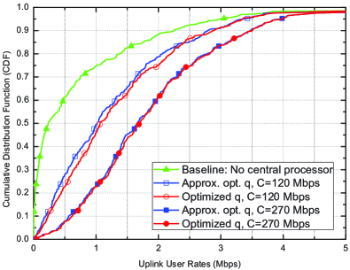
Figure 2: Cumulative distribution of user rates with the VMAC-WZ scheme

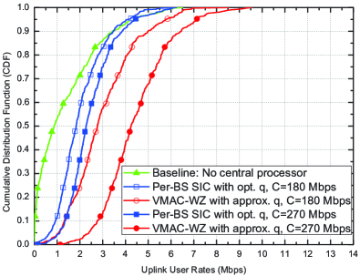
Figure 3: Performance comparison of the VMAC-WZ scheme with the per-BS interference cancellation scheme of [12].

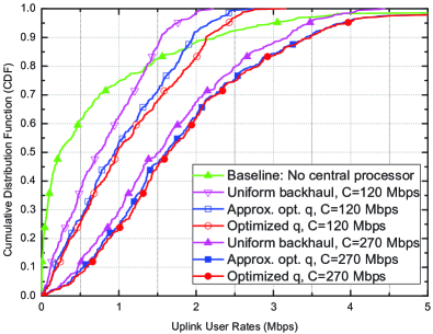
Figure 4: Cumulative distribution of user rates with the VMAC-SU scheme

Fig. 4 shows the CDF curves of user rates for the VMAC-SU scheme with three choices of quantization noise levels: the quantization noise levels given by allocating the backhaul capacity equally across the BSs (labeled as “uniform backhaul”), the approximately optimal $q_{i}$ proportional to the background noise as given by Algorithm 3 (labeled as “approx. opt. q”), and the optimal $q_{i}$ derived from the backhaul capacity allocation formulation of the problem (labeled as “optimized q”). It can be seen that VMAC with single-user compression also significantly improves the performance of baseline system and that the approximately optimal $q_{i}$ is near optimal, especially when $C$ is large. The figure also shows that allocating backhaul capacity uniformly across the BSs is strictly suboptimal.

To further compare the performance of the VMAC-SU scheme with different choices of quantization noise levels, Fig. 5 plots the average per-cell sum rate of the baseline and the VMAC-SU schemes as a function of the backhaul capacity. The figure clearly shows the advantage of optimizing the quantization noise levels (or equivalently the allocation of backhaul capacities). For example, to achieve $80$Mbps per-cell sum rate, we need $200$Mbps sum backhaul if backhaul capacities are allocated uniformly, $170$Mbps sum backhaul if $q_{i}$ is chosen to be proportional to the background noise, and $150$Mbps sum backhaul if $q_{i}$ is optimized. Thus, the optimization of the quantization noise level can save up to 25% in backhaul capacity.

Further, it can be seen from Fig. 5 that under infinite sum backhaul, the achieved per-cell sum rate saturates and approaches about $115$Mbps for this cellular setting. But when the quantization noise level is optimized, a finite sum backhaul capacity at about $200$Mbps is already sufficient to achieve about $100$Mbps user sum rate, which is $90\%$ of the full benefit of uplink network MIMO. Note that the performance gap between the approximately optimal $q_{i}$ and the optimal $q_{i}$ becomes smaller as the sum backhaul capacity increases, confirming the approximate optimality of $q_{i}=\alpha\sigma_{i}^{2}$ in the high SQNR regime.

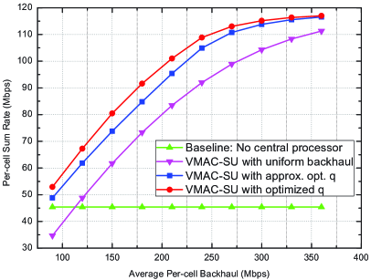
Figure 5: Per-cell sum rate vs. average per-cell backhaul capacity of the VMAC-SU scheme.

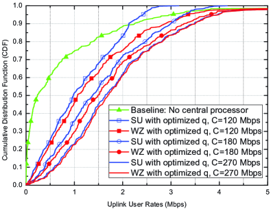
Figure 6: Comparison of the VMAC-SU and VMAC-WZ schemes

Fig. 6 compares the performance of Wyner-Ziv coding and single-user compression for the VMAC scheme. It is observed that Wyner-Ziv coding is superior to single-use compression. However, as the sum backhaul capacity becomes larger, the gain due to Wyner-Ziv coding diminishes.

V-B Multi-Tier Heterogeneous Network

TABLE II: Heterogeneous Network Channel Parameters

Cellular Layout	Hexagonal, wrapped around
BS-to-BS Distance	$500$ m
Number of Macro Cells	$7$ cells, $3$ sectors/cell
Number of Pico Cells	$3$ pico cells per macro sector
Frequency Reuse	$1$
Channel Bandwidth	$10$ MHz
Number of Users per
Macro Sector	$20$
User Transmit Power	$23$ dBm
Antenna Gain	14 dBi
Background Noise	$-169$ dBm/Hz
Noise Figure	$7$ dB
Pico BS Antenna Pattern	Omni-directional
Tx/Rx Antenna No.	$1$
Path Loss Macro to User	$128.1+37.6\log_{10}(d)$
Path Loss Pico to User	$140.7+36.7\log_{10}(d)$
	$8$ dB standard deviation
Log-normal Shadowing	for macro-user link;
	$4$ dB for pico-user link
Shadow Fading Correlation	$0.5$
Cluster Size	$1$ macro cell and $9$ pico cells
Min. Dist. between BSs	$75$ m
Scheduling Strategy	Round-robin

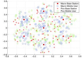
Figure 7: A picocell network topology with $7$ cells, $3$ sectors per cell, and $3$ pico base-stations per sector placed randomly.

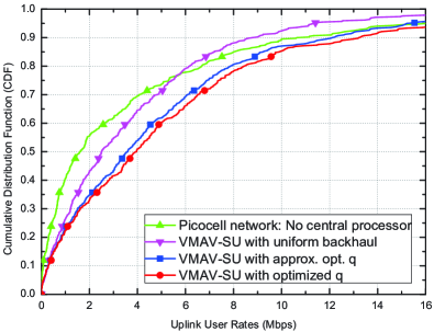
Figure 8: Cumulative distribution of user rates in the picocell network where the 3 macro-BSs and 9 pico-BSs within each 3-sector macrocell form a cluster. The VMAC-SU scheme is applied and the sum backhaul constraints for macro and pico BSs are $189$Mpbs and $81$Mpbs per cluster, respectively.

The performance of the VMAC-SU scheme is further evaluated for a two-tier heterogeneous network with $7$ macro-cells wrapped around, $3$ sectors per cell, $3$ pico BSs randomly located in each sector, and $20$ mobile users per macro-cell sector. The cellular topology is shown in Fig. 7. Each user establishes connection with the macro/pico BS with the highest received SNR. Note that the number of users in each pico/macro-cell is not fixed. On average there are $8$ users per macro-cell sector and $4$ users per pico-cell. In this network, every macro-cell forms a C-RAN cluster, consisting of $3$ macro-sectors and $9$ pico-cells. The macro BSs and pico BSs are subject to different sum backhaul capacity constraints. Specifically, the sum backhaul capacity is set to be $189$Mbps for the $3$ macro-BSs and $81$Mbps for the $9$ pico BSs. Perfect CSI is made available to all the BSs and to the CP. System parameters are outlined in Table II.

Fig. 8 shows the CDF plots of user rates achieved by the baseline scheme and the VMAC-SU scheme. It is clear that the C-RAN architecture significantly improves upon the baseline, more than doubling the $50$-percentile rate. The optimization of the quantization noise level is important, as a naive uniform backhaul allocation only achieves half of the potential gain for C-RAN. Finally, setting the quantization noise level to be proportional to the background noise is indeed approximately optimal. In this multi-tier heterogeneous network case, the proportionality constant is set independently for each tier using Algorithm 3.

VI Conclusion

This paper studies an uplink C-RAN model where the BSs within a cooperation cluster are connected to a cloud-computing based CP through noiseless backhaul links of limited sum capacity. We employ two VMAC schemes where the BSs use either Wyner-Ziv compression or single-user compression to quantize the received signals and send the compressed bits to the CP. At the CP, quantization codewords are first decoded; subsequently the user messages are decoded as if the users form a virtual multiple-access channel.

The main findings of the paper are concerned with efficient optimization of the quantization noise levels for both VMAC-WZ and VMAC-SU. We propose an alternating optimization algorithm for VMAC-WZ and a backhaul capacity allocation formulation for VMAC-SU. More importantly, it is observed that setting the quantization noise levels to be proportional to the background noise levels is approximately optimal. This leads to efficient algorithms for optimizing the quantization noise levels, or equivalently, for allocating the backhaul capacities.

From an analytic point of view, this paper shows that setting quantization noise levels to be proportional to the background noise levels is near optimal for maximizing the sum rate when the system operates in the high SQNR regime. With such a choice of quantization noise levels, the VMAC-WZ scheme can achieve the sum capacity of the uplink C-RAN model to within a constant gap. A similar constant-gap result is also obtained for VMAC-SU under a diagonally dominant channel condition. From a numerical perspective, simulation results confirm that the proposed VMAC schemes can significantly improve the performance of wireless cellular systems. The improvement is maximized with optimized quantization noise levels or equivalently optimized backhaul capacity allocations. The near optimal choice of quantization noise levels indeed performs very close to the optimal one over the SQNR region of practical interest.

Appendix A Proof of Theorem 2

The idea is to choose $q_{i}=\alpha\sigma_{i}^{2}$, $i=1,2,\ldots,L$ where $\alpha>0$ is an appropriately chosen constant, then compare the achievable rate of VMAC-WZ with the following cut-set like sum-capacity upper bound [7]

$$\bar{C}=\min\left\{\log\frac{\left|\mathbf{H}K_{X}\mathbf{H}^{H}+\mathrm{diag}(\sigma^{2}_{i})\right|}{\left|\mathrm{diag}(\sigma^{2}_{i})\right|},C\right\}$$ (33)

where the first term is the cut from the users to the BSs, and the second term is the cut across the backhaul links.

We choose the quantization noise level $\alpha$ depending on $C$ as follows: When $C\geq\log\frac{\left|\mathbf{H}K_{X}\mathbf{H}^{H}+2\mathrm{diag}(\sigma^{2}_{i})\right|}{\left|\mathrm{diag}(\sigma^{2}_{i})\right|}$, we choose $\alpha=1$, i.e., the quantization noise levels are set to be at the background noise levels. Since $\alpha=1$, it can be verified that

$$I(\mathbf{Y};\widehat{\mathbf{Y}})=\log\frac{\left|\mathbf{H}K_{X}\mathbf{H}^{H}+2\mathrm{diag}(\sigma^{2}_{i})\right|}{\left|\mathrm{diag}(\sigma^{2}_{i})\right|}.$$ (34)

Thus, we have $C\geq I(\mathbf{Y};\widehat{\mathbf{Y}})$. This implies that the sum backhaul constraint (2) is satisfied. Therefore, the sum rate

$$R_{sum}=I(\mathbf{X};\widehat{\mathbf{Y}})=\log\frac{\left|\mathbf{H}K_{X}\mathbf{H}^{H}+2\mathrm{diag}(\sigma^{2}_{i})\right|}{\left|2\mathrm{diag}(\sigma^{2}_{i})\right|}$$ (35)

is achievable. In this case, the gap between $\bar{C}$ and $R_{sum}$ can be bounded by

$$\bar{C}-R_{sum} \leq \log\frac{\left|\mathbf{H}K_{X}\mathbf{H}^{H}+\mathrm{diag}(\sigma^{2}_{i})\right|}{\left|\mathrm{diag}(\sigma^{2}_{i})\right|}$$

$$-\log\frac{\left|\mathbf{H}K_{X}\mathbf{H}^{H}+2\mathrm{diag}(\sigma^{2}_{i})\right|}{\left|2\mathrm{diag}(\sigma^{2}_{i})\right|}<L.$$

When $C<\log\frac{\left|\mathbf{H}K_{X}\mathbf{H}^{H}+2\mathrm{diag}(\sigma^{2}_{i})\right|}{\left|\mathrm{diag}(\sigma^{2}_{i})\right|}$, we choose $\alpha$ such that $I(\mathbf{Y};\widehat{\mathbf{Y}})=C$. First, note that for such a choice of $\alpha$ the sum rate $R_{sum}=I(\mathbf{X};\widehat{\mathbf{Y}})$ is achievable. Next, observe that

$$I(\mathbf{Y};\widehat{\mathbf{Y}})=\log\frac{\left|\mathbf{H}K_{X}\mathbf{H}^{H}+\mathrm{diag}(\sigma^{2}_{i})+\alpha\mathrm{diag}(\sigma^{2}_{i})\right|}{\left|\alpha\mathrm{diag}(\sigma^{2}_{i})\right|}$$ (36)

is a monotonically decreasing function of $\alpha$. Since $C=I(\mathbf{Y};\widehat{\mathbf{Y}})<\log\frac{\left|\mathbf{H}K_{X}\mathbf{H}^{H}+2\mathrm{diag}(\sigma^{2}_{i})\right|}{\left|\mathrm{diag}(\sigma^{2}_{i})\right|}$, we have $\alpha>1$. Now, we use $C=I(\mathbf{Y};\widehat{\mathbf{Y}})$ as an upper bound. The gap between $\bar{C}$ and $R_{sum}$ can be bounded by

$$\bar{C}-R_{sum} \leq I(\mathbf{Y};\widehat{\mathbf{Y}})-I(\mathbf{X};\widehat{\mathbf{Y}})$$

$$= \log\frac{\left|\mathbf{H}K_{X}\mathbf{H}^{H}+(1+\alpha)\mathrm{diag}(\sigma^{2}_{i})\right|}{\left|\alpha\mathrm{diag}(\sigma^{2}_{i})\right|}$$

$$-\log\frac{\left|\mathbf{H}K_{X}\mathbf{H}^{H}+(1+\alpha)\mathrm{diag}(\sigma^{2}_{i})\right|}{\left|(1+\alpha)\mathrm{diag}(\sigma^{2}_{i})\right|}$$

$$= L\log\left(1+\frac{1}{\alpha}\right)<L$$

where the last inequality follows from the fact that $\alpha>1$.

Combining the two cases, we see that the gap to the sum capacity for the VMAC-WZ scheme with appropriately chosen quantization noise levels (which are proportional to the background noise levels) is always less than $1$ bit per BS per channel use.

Appendix B Proof of Theorem 3

Lemma 2

For fixed $\kappa>1$, suppose that a $n\times n$ matrix $\Psi$ is $\kappa$-strictly diagonally dominant, then

$$\left|\Psi\right|\geq\left(1-\frac{1}{\kappa}\right)^{n}\prod_{i=1}^{n}|\Psi(i,i)|.$$ (37)

Proof:

The proof follows from the lower bound given in [25], which shows that if $\Psi$ is strictly diagonally dominant, i.e. $|\Psi(i,i)|>\sum\limits_{j\neq i}^{n}|\Psi(i,j)|$ for $i=1,\ldots,n$, then the determinant of $\Psi$ can be bounded from below as follows,

$$|\Psi|\geq\prod_{i=1}^{n}\left(|\Psi(i,i)|-\sum_{j\neq i}^{n}|\Psi(i,j)|\right).$$ (38)

Under the condition that $\Psi$ is $\kappa$-strictly diagonally dominant, i.e. $\sum_{j\neq i}^{n}|\Psi(i,j)|\leq\frac{|\Psi(i,i)|}{\kappa}$ we further bound $|\Psi|$ by

$$|\Psi| \geq \prod_{i=1}^{n}\left(|\Psi(i,i)|-\frac{|\Psi(i,i)|}{\kappa}\right)$$ (39)

$$= \left(1-\frac{1}{\kappa}\right)^{n}\prod_{i=1}^{n}|\Psi(i,i)|,$$

which completes the proof. ∎

We now prove Theorem 3. The proof uses the same technique as in that of Theorem 2. We first choose the quantization noise levels $q_{i}=\alpha\sigma^{2}_{i}$, $i=1,2,\ldots,L$, where $\alpha>0$ is a constant depending on $C$, then compare the achievable rate of the VMAC-SU scheme with the following cut-set like upper bound [7]

$$\bar{C}=\min\left\{\log\frac{\left|\mathbf{H}K_{X}\mathbf{H}^{H}+\mathrm{diag}(\sigma^{2}_{i})\right|}{\left|\mathrm{diag}(\sigma^{2}_{i})\right|},C\right\}.$$ (40)

We consider two different cases as follows: when $C\geq\log\frac{\left|\mathrm{diag}(\mathbf{H}K_{X}\mathbf{H}^{H})+2\mathrm{diag}(\sigma^{2}_{i})\right|}{\left|\mathrm{diag}(\sigma^{2}_{i})\right|}$, i.e. the sum backhaul capacity is large enough to support the choice of $q_{i}=\sigma_{i}^{2}$, we choose $\alpha=1$. In this case, the gap between $\bar{C}$ and $R_{sum}$ can be bounded by

$$\bar{C}-R_{sum} \leq \log\frac{\left|\mathbf{H}K_{X}\mathbf{H}^{H}+\mathrm{diag}(\sigma^{2}_{i})\right|}{\left|\mathrm{diag}(\sigma^{2}_{i})\right|}$$

$$-\log\frac{\left|\mathbf{H}K_{X}\mathbf{H}^{H}+2\mathrm{diag}(\sigma^{2}_{i})\right|}{\left|2\mathrm{diag}(\sigma^{2}_{i})\right|}<L.$$

When $C<\log\frac{\left|\mathrm{diag}(\mathbf{H}K_{X}\mathbf{H}^{H})+2\mathrm{diag}(\sigma^{2}_{i})\right|}{\left|\mathrm{diag}(\sigma^{2}_{i})\right|}$, we choose $\alpha$ so that $\sum_{i=1}^{L}I(Y_{i};\hat{Y}_{i})=C$. First, notice that

$$\sum_{i=1}^{L}I(Y_{i};\hat{Y}_{i})=\log\frac{\left|\mathrm{diag}(\mathbf{H}K_{X}\mathbf{H}^{H})+(1+\alpha)\mathrm{diag}(\sigma^{2}_{i})\right|}{\left|\alpha\mathrm{diag}(\sigma^{2}_{i})\right|}$$

is a monotonically decreasing function of $\alpha$. Since $C=\sum_{i=1}^{L}I(Y_{i};\hat{Y}_{i})<\log\frac{\left|\mathrm{diag}(\mathbf{H}K_{X}\mathbf{H}^{H})+2\mathrm{diag}(\sigma^{2}_{i})\right|}{\left|\mathrm{diag}(\sigma^{2}_{i})\right|}$, we have $\alpha>1$. Now, we use $C=\sum_{i=1}^{L}I(Y_{i};\hat{Y}_{i})$ as an upper bound. Let $\Omega=\mathbf{H}K_{X}\mathbf{H}^{H}+(1+\alpha)\mathrm{diag}(\sigma^{2}_{i})$ and note that $\Omega(i,i)\geq 0$. The gap between $\bar{C}$ and $R_{sum}$ is bounded by

$$\bar{C}-R_{sum} \leq \sum_{i=1}^{L}I(Y_{i};\hat{Y}_{i})-I(\mathbf{X};\widehat{\mathbf{Y}})$$

$$= \log\frac{\left|\mathrm{diag}(\mathbf{H}K_{X}\mathbf{H}^{H})+(1+\alpha)\mathrm{diag}(\sigma^{2}_{i})\right|}{\left|\alpha\mathrm{diag}(\sigma^{2}_{i})\right|}$$

$$-\log\frac{\left|\mathbf{H}K_{X}\mathbf{H}^{H}+(1+\alpha)\mathrm{diag}(\sigma^{2}_{i})\right|}{\left|(1+\alpha)\mathrm{diag}(\sigma^{2}_{i})\right|}$$

$$= \log\left[\left(1+\frac{1}{\alpha}\right)^{L}\frac{\prod\limits_{i=1}^{L}\Omega(i,i)}{|\Omega|}\right].$$

Since matrix $\mathbf{H}K_{X}\mathbf{H}^{H}+\mathrm{diag}(\sigma^{2}_{i})$ is $\kappa$-strictly diagonally dominant, $\Omega$ is also $\kappa$-strictly diagonally dominant. Following the result of Lemma 2, we further bound the gap as follows,

$$\bar{C}-R_{sum} \leq L\log\left(1+\frac{1}{\alpha}\right)+\sum_{i=1}^{L}\log\frac{\kappa}{\kappa-1}$$

$$< L\left(1+\log\frac{\kappa}{\kappa-1}\right),$$

where the last inequality follows from the fact that $\alpha>1$.

Combining the two cases, we see that the gap to sum capacity for the VMAC-SU scheme with quantization noise levels proportional to the background noise levels is always less than $1+\log\frac{\kappa}{\kappa-1}$ per BS per channel use.

Yuhan Zhou (S’08) received the B.E. degree in Electronic and Information Engineering from Jilin University, Chuangchun, Jilin, China, in 2005 and M.A.Sc. degree in Electrical and Computer Engineering from the University of Waterloo, Waterloo, Ontario, Canada, in 2009. He is currently working towards the Ph.D. degree with the Electrical and Computer Engineering Department at the University of Toronto, Toronto, Ontario, Canada. His research interests include wireless communications, network information theory, and convex optimization.

Wei Yu (S’97-M’02-SM’08-F’14) received the B.A.Sc. degree in Computer Engineering and Mathematics from the University of Waterloo, Waterloo, Ontario, Canada in 1997 and M.S. and Ph.D. degrees in Electrical Engineering from Stanford University, Stanford, CA, in 1998 and 2002, respectively. Since 2002, he has been with the Electrical and Computer Engineering Department at the University of Toronto, Toronto, Ontario, Canada, where he is now Professor and holds a Canada Research Chair (Tier 1) in Information Theory and Wireless Communications. His main research interests include information theory, optimization, wireless communications and broadband access networks. Prof. Wei Yu served as an Associate Editor for IEEE Transactions on Information Theory (2010-2013), as an Editor for IEEE Transactions on Communications (2009-2011), as an Editor for IEEE Transactions on Wireless Communications (2004-2007), and as a Guest Editor for a number of special issues for the IEEE Journal on Selected Areas in Communications and the EURASIP Journal on Applied Signal Processing. He was a Technical Program Committee (TPC) co-chair of the Communication Theory Symposium at the IEEE International Conference on Communications (ICC) in 2012, and a TPC co-chair of the IEEE Communication Theory Workshop in 2014. He was a member of the Signal Processing for Communications and Networking Technical Committee of the IEEE Signal Processing Society (2008-2013). Prof. Wei Yu received an IEEE ICC Best Paper Award in 2013, an IEEE Signal Processing Society Best Paper Award in 2008, the McCharles Prize for Early Career Research Distinction in 2008, the Early Career Teaching Award from the Faculty of Applied Science and Engineering, University of Toronto in 2007, and an Early Researcher Award from Ontario in 2006. Prof. Wei Yu was named as a Highly Cited Researcher by Thomson Reuters in 2014. He is a registered Professional Engineer in Ontario.

References

- [1] Y. Zhou and W. Yu, “Approximate bounds for limited backhaul uplink multicell processing with single-user compression,” in Proc. IEEE Canadian Workshop on Inf. Theory (CWIT), Jun. 2013, pp. 113–116.
- [2] Y. Zhou, W. Yu, and D. Toumpakaris, “Uplink multi-cell processing: Approximate sum capacity under a sum backhaul constraint,” in Proc. IEEE Inf. Theory Workshop (ITW), Sep. 2013, pp. 569–573.
- [3] D. Gesbert, S. Hanly, H. Huang, S. Shamai, O. Simeone, and W. Yu, “Multi-cell MIMO cooperative networks: A new look at interference,” IEEE J. Sel. Areas Commun., vol. 28, no. 9, pp. 1380–1408, Dec. 2010.
- [4] O. Somekh, B. M. Zaidel, and S. Shamai, “Sum rate characterization of joint multiple cell-site processing,” IEEE Trans. Inf. Theory, vol. 53, no. 12, pp. 4473–4497, Dec. 2007.
- [5] O. Simeone, O. Somekh, H. V. Poor, and S. Shamai, “Local base station cooperation via finite-capacity links for the uplink of linear cellular networks,” IEEE Trans. Inf. Theory, vol. 55, no. 1, pp. 190–204, Jan. 2009.
- [6] A. Sanderovich, S. Shamai, Y. Steinberg, and G. Kramer, “Communication via decentralized processing,” IEEE Trans. Inf. Theory, vol. 54, no. 7, pp. 3008–3023, Jul. 2008.
- [7] A. Sanderovich, O. Somekh, H. V. Poor, and S. Shamai, “Uplink macro diversity of limited backhaul cellular network,” IEEE Trans. Inf. Theory, vol. 55, no. 8, pp. 3457–3478, Aug. 2009.
- [8] A. Sanderovich, S. Shamai, and Y. Steinberg, “Distributed MIMO receiver–Achievable rates and upper bounds,” IEEE Trans. Inf. Theory, vol. 55, no. 10, pp. 4419–4438, Oct. 2009.
- [9] A. Avestimehr, S. Diggavi, and D. Tse, “Wireless network information flow: A deterministic approach,” IEEE Trans. Inf. Theory, vol. 57, no. 4, pp. 1872–1905, Apr. 2011.
- [10] S. H. Lim, Y.-H. Kim, A. El Gamal, and S.-Y. Chung, “Noisy network coding,” IEEE Trans. Inf. Theory, vol. 57, no. 5, pp. 3132–3152, May 2011.
- [11] M. H. Yassaee and M. R. Aref, “Slepian–Wolf coding over cooperative relay networks,” IEEE Trans. Inf. Theory, vol. 57, no. 6, pp. 3462–3482, Jun. 2011.
- [12] L. Zhou and W. Yu, “Uplink multicell processing with limited backhaul via per-base-station successive interference cancellation,” IEEE J. Sel. Areas Commun., vol. 31, no. 10, pp. 1981–1993, Oct. 2013.
- [13] A. del Coso and S. Simoens, “Distributed compression for MIMO coordinated networks with a backhaul constraint,” IEEE Trans. Wireless Commun., vol. 8, no. 9, pp. 4698–4709, Sep. 2009.
- [14] S.-H. Park, O. Simeone, O. Sahin, and S. Shamai, “Robust and efficient distributed compression for cloud radio access networks,” IEEE Trans. Veh. Commun., vol. 62, no. 2, pp. 692–703, Feb. 2013.
- [15] P. Marsch and G. Fettweis, “Uplink CoMP under a constrained backhaul and imperfect channel knowledge,” IEEE Trans. Wireless Commun., vol. 10, no. 6, pp. 1730–1742, Jun. 2011.
- [16] R. Karasik, O. Simeone, and S. Shamai, “Robust uplink communications over fading channels with variable backhaul connectivity,” IEEE Trans. Wireless Commun., 2013. [Online]. Available: http://arxiv.org/abs/1301.6938
- [17] B. Nazer, A. Sanderovich, M. Gastpar, and S. Shamai, “Structured superposition for backhaul constrained cellular uplink,” in Proc. IEEE Int. Symp. Inf. Theory (ISIT), Jun. 2009, pp. 1530–1534.
- [18] S.-N. Hong and G. Caire, “Compute-and-forward strategies for cooperative distributed antenna systems,” IEEE Trans. Inf. Theory, vol. 59, no. 9, pp. 5227–5243, Sep. 2013.
- [19] M. Razaviyayn, M. Hong, and Z.-Q. Luo, “A unified convergence analysis of block successive minimization methods for nonsmooth optimization,” SIAM J. Optim., vol. 23, no. 2, pp. 1126–1153, Feb. 2013.
- [20] D. R. Hunter and K. Lange, “A tutorial on MM algorithms,” Am. Stat., vol. 58, no. 1, pp. 30–37, Jan. 2004.
- [21] Q. Li, M. Hong, H.-T. Wai, Y.-F. Liu, W.-K. Ma, and Z.-Q. Luo, “Transmit solutions for MIMO wiretap channels using alternating optimization,” IEEE J. Sel. Areas Commun., vol. 31, no. 9, pp. 1714–1727, 2013.
- [22] M. Hong, Q. Li, and Y.-F. Liu, “Decomposition by successive convex approximation: A unifying approach for linear transceiver design in interfering heterogeneous networks,” submitted to IEEE Trans. Signal Process., 2012. [Online]. Available: http://arxiv.org/abs/1210.1507
- [23] L. Grippo and M. Sciandrone, “On the convergence of the block nonlinear Gauss–Seidel method under convex constraints,” Oper. Res. Lett., vol. 26, no. 3, pp. 127–136, Mar. 2000.
- [24] A. Beck and L. Tetruashvili, “On the convergence of block coordinate descent type methods,” SIAM J. Optim., vol. 23, no. 4, pp. 2037–2060, Apr. 2013.
- [25] A. M. Ostrowski, “Note on bounds for determinants with dominant principal diagonal,” Proc. Amer. Math. Soc., vol. 3, no. 1, pp. 26–30, 1952.