Deterministic Initialization of the K-Means Algorithm Using Hierarchical Clustering

Abstract

K-means is undoubtedly the most widely used partitional clustering algorithm. Unfortunately, due to its gradient descent nature, this algorithm is highly sensitive to the initial placement of the cluster centers. Numerous initialization methods have been proposed to address this problem. Many of these methods, however, have superlinear complexity in the number of data points, making them impractical for large data sets. On the other hand, linear methods are often random and/or order-sensitive, which renders their results unrepeatable. Recently, Su and Dy proposed two highly successful hierarchical initialization methods named Var-Part and PCA-Part that are not only linear, but also deterministic (non-random) and order-invariant. In this paper, we propose a discriminant analysis based approach that addresses a common deficiency of these two methods. Experiments on a large and diverse collection of data sets from the UCI Machine Learning Repository demonstrate that Var-Part and PCA-Part are highly competitive with one of the best random initialization methods to date, i.e., k-means++, and that the proposed approach significantly improves the performance of both hierarchical methods.

1 Introduction

Clustering, the unsupervised classification of patterns into groups, is one of the most important tasks in exploratory data analysis [1]. Primary goals of clustering include gaining insight into data (detecting anomalies, identifying salient features, etc.), classifying data, and compressing data. Clustering has a long and rich history in a variety of scientific disciplines including anthropology, biology, medicine, psychology, statistics, mathematics, engineering, and computer science. As a result, numerous clustering algorithms have been proposed since the early 1950s [2].

Clustering algorithms can be broadly classified into two groups: hierarchical and partitional [2]. Hierarchical algorithms recursively find nested clusters either in a top-down (divisive) or bottom-up (agglomerative) fashion. In contrast, partitional algorithms find all the clusters simultaneously as a partition of the data and do not impose a hierarchical structure. Most hierarchical algorithms have quadratic or higher complexity in the number of data points [1] and therefore are not suitable for large data sets, whereas partitional algorithms often have lower complexity.

Given a data set ${\mathcal{X}}=\{{\bf x}_{1},{\bf x}_{2},\dotsc,{\bf x}_{N}\}$ in $\mathbb{R}^{D}$, i.e., $N$ points (vectors) each with $D$ attributes (components), hard partitional algorithms divide ${\mathcal{X}}$ into $K$ exhaustive and mutually exclusive clusters $\mathcal{P}=\{P_{1},P_{2},\dotsc,P_{K}\},$ $\;\;\bigcup\nolimits_{i=1}^{K}{P_{i}={\mathcal{X}}},$ $\;\;P_{i}\cap P_{j}=\emptyset$ for $1\leq i\neq j\leq K$. These algorithms usually generate clusters by optimizing a criterion function. The most intuitive and frequently used criterion function is the Sum of Squared Error (SSE) given by:

$$\mbox{SSE}=\sum\limits_{i=1}^{K}{\sum\limits_{{\bf x}_{j}\in P_{i}}{\left\|{{\bf x}_{j}-{\bf c}_{i}}\right\|_{2}^{2}}}$$ (1)

where $\|.\|_{2}$ denotes the Euclidean ($\mathcal{L}_{2}$) norm and ${\bf c}_{i}={1\mathord{\left/{\vphantom{1{\left|P_{i}\right|}}}\right.\kern-1.2pt}{\left|P_{i}\right|}}\sum\nolimits_{{\bf x}_{j}\in P_{i}}{{\bf x}_{j}}$ is the centroid of cluster $P_{i}$ whose cardinality is $\left|P_{i}\right|$. The optimization of (1) is often referred to as the minimum SSE clustering (MSSC) problem.

The number of ways in which a set of $N$ objects can be partitioned into $K$ non-empty groups is given by Stirling numbers of the second kind:

$$\mathcal{S}(N,K)=\frac{1}{{K!}}\sum\limits_{i=0}^{K}{(-1)^{K-i}\left(\begin{gathered}K\hfill\\ i\hfill\\ \end{gathered}\right)}i^{N}$$ (2)

which can be approximated by $K^{N}/K!$ It can be seen that a complete enumeration of all possible clusterings to determine the global minimum of (1) is clearly computationally prohibitive except for very small data sets [3]. In fact, this non-convex optimization problem is proven to be NP-hard even for $K=2$ [4] or $D=2$ [5]. Consequently, various heuristics have been developed to provide approximate solutions to this problem [6]. Among these heuristics, Lloyd’s algorithm [7], often referred to as the (batch) k-means algorithm, is the simplest and most commonly used one. This algorithm starts with $K$ arbitrary centers, typically chosen uniformly at random from the data points. Each point is assigned to the nearest center and then each center is recalculated as the mean of all points assigned to it. These two steps are repeated until a predefined termination criterion is met.

The k-means algorithm is undoubtedly the most widely used partitional clustering algorithm [2]. Its popularity can be attributed to several reasons. First, it is conceptually simple and easy to implement. Virtually every data mining software includes an implementation of it. Second, it is versatile, i.e., almost every aspect of the algorithm (initialization, distance function, termination criterion, etc.) can be modified. This is evidenced by hundreds of publications over the last fifty years that extend k-means in various ways. Third, it has a time complexity that is linear in $N$, $D$, and $K$ (in general, $D\ll N$ and $K\ll N$). For this reason, it can be used to initialize more expensive clustering algorithms such as expectation maximization [8], DBSCAN [9], and spectral clustering [10]. Furthermore, numerous sequential [11, 12] and parallel [13] acceleration techniques are available in the literature. Fourth, it has a storage complexity that is linear in $N$, $D$, and $K$. In addition, there exist disk-based variants that do not require all points to be stored in memory [14]. Fifth, it is guaranteed to converge [15] at a quadratic rate [16]. Finally, it is invariant to data ordering, i.e., random shufflings of the data points.

On the other hand, k-means has several significant disadvantages. First, it requires the number of clusters, $K$, to be specified in advance. The value of this parameter can be determined automatically by means of various internal/relative cluster validity measures [17]. Second, it can only detect compact, hyperspherical clusters that are well separated. This can be alleviated by using a more general distance function such as the Mahalanobis distance, which permits the detection of hyperellipsoidal clusters [18]. Third, due its utilization of the squared Euclidean distance, it is sensitive to noise and outlier points since even a few such points can significantly influence the means of their respective clusters. This can be addressed by outlier pruning [19] or using a more robust distance function such as City-block ($\mathcal{L}_{1}$) distance. Fourth, due to its gradient descent nature, it often converges to a local minimum of the criterion function [15]. For the same reason, it is highly sensitive to the selection of the initial centers [20]. Adverse effects of improper initialization include empty clusters, slower convergence, and a higher chance of getting stuck in bad local minima [21]. Fortunately, except for the first two, these drawbacks can be remedied by using an adaptive initialization method (IM).

A large number of IMs have been proposed in the literature [22, 23, 21, 20]. Unfortunately, many of these have superlinear complexity in $N$ [24, 25, 26, 3, 27, 28, 29, 30, 31, 32], which makes them impractical for large data sets (note that k-means itself has linear complexity). In contrast, linear IMs are often random and/or order-sensitive [33, 34, 35, 36, 37, 38, 8, 39], which renders their results unrepeatable. Su and Dy proposed two divisive hierarchical initialization methods named Var-Part and PCA-Part that are not only linear, but also deterministic and order-invariant [40]. In this study, we propose a simple modification to these methods that improves their performance significantly.

The rest of the paper is organized as follows. Section 2 presents a brief overview of some of the most popular linear, order-invariant k-means IMs and the proposed modification to Var-Part and PCA-Part. Section 3 presents the experimental results, while Section 4 analyzes these results. Finally, Section 5 gives the conclusions.

2 Linear, Order-Invariant Initialization Methods for K-Means

2.1 Overview of the Existing Methods

Forgy’s method [33] assigns each point to one of the $K$ clusters uniformly at random. The centers are then given by the centroids of these initial clusters. This method has no theoretical basis, as such random clusters have no internal homogeneity [41].

MacQueen [35] proposed two different methods. The first one, which is the default option in the Quick Cluster procedure of IBM SPSS Statistics [42], takes the first $K$ points in ${\mathcal{X}}$ as the centers. An obvious drawback of this method is its sensitivity to data ordering. The second method chooses the centers randomly from the data points. The rationale behind this method is that random selection is likely to pick points from dense regions, i.e., points that are good candidates to be centers. However, there is no mechanism to avoid choosing outliers or points that are too close to each other [41]. Multiple runs of this method is the standard way of initializing k-means [8]. It should be noted that this second method is often mistakenly attributed to Forgy [33].

The maximin method [43] chooses the first center ${\bf c}_{1}$ arbitrarily and the $i$-th ($i\in\{2,3,\dotsc,K\}$) center ${\bf c}_{i}$ is chosen to be the point that has the greatest minimum-distance to the previously selected centers, i.e., ${\bf c}_{1},{\bf c}_{2},\dotsc,{\bf c}_{i-1}$. This method was originally developed as a $2$-approximation to the $K$-center clustering problem.

The k-means++ method [39] interpolates between MacQueen’s second method and the maximin method. It chooses the first center randomly and the $i$-th ($i\in\{2,3,\dotsc,K\}$) center is chosen to be ${\bf x}^{\prime}\in{\mathcal{X}}$ with a probability of $\frac{{md\left({{\bf x}^{\prime}}\right)^{2}}}{{\sum\nolimits_{j=1}^{N}{md({\bf x}_{j})^{2}}}}$, where $md({\bf x})$ denotes the minimum-distance from a point ${\bf x}$ to the previously selected centers. This method yields an $\Theta(\log{K})$ approximation to the MSSC problem.

The PCA-Part method [40] uses a divisive hierarchical approach based on PCA (Principal Component Analysis) [44]. Starting from an initial cluster that contains the entire data set, the method iteratively selects the cluster with the greatest SSE and divides it into two subclusters using a hyperplane that passes through the cluster centroid and is orthogonal to the principal eigenvector of the cluster covariance matrix. This procedure is repeated until $K$ clusters are obtained. The centers are then given by the centroids of these clusters. The Var-Part method [40] is an approximation to PCA-Part, where the covariance matrix of the cluster to be split is assumed to be diagonal. In this case, the splitting hyperplane is orthogonal to the coordinate axis with the greatest variance.

Figure 1 illustrates the Var-Part procedure on a toy data set with four natural clusters [45]. In iteration $1$, the initial cluster that contains the entire data set is split into two subclusters along the Y axis using a line (one-dimensional hyperplane) that passes through the mean point ($92.026667$). Between the resulting two clusters, the one above the line has a greater SSE. In iteration $2$, this cluster is therefore split along the X axis at the mean point ($66.975000$). In the final iteration, the cluster with the greatest SSE, i.e., the bottom cluster, is split along the X axis at the mean point ($41.057143$). In Figure 1(d), the centroids of the final four clusters are denoted by stars.

(a) Input data set

(b) Iteration 1

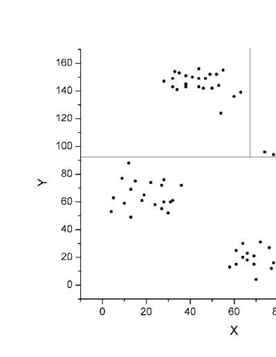
(c) Iteration 2

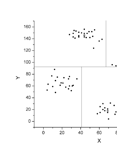
(d) Iteration 3

Figure 1: Illustration of Var-Part on the Ruspini data set

2.2 Proposed Modification to Var-Part and PCA-Part

Su and Dy [40] demonstrated that, besides being computationally efficient, Var-Part and PCA-Part perform very well on a variety of data sets. Recall that in each iteration these methods select the cluster with the greatest SSE and then project the $D$-dimensional points in this cluster on a partitioning axis. The difference between the two methods is the choice of this axis. In Var-Part, the partitioning axis is the coordinate axis with the greatest variance, whereas in PCA-Part it is the major axis. After the projection operation, both methods use the mean point on the partitioning axis as a ‘threshold’ to divide the points between two clusters. In other words, each point is assigned to one of the two subclusters depending on which side of the mean point its projection falls to. It should be noted that the choice of this threshold is primarily motivated by computational convenience. Here, we propose a better alternative based on discriminant analysis.

The projections of the points on the partitioning axis can be viewed as a discrete probability distribution, which can be conveniently represented by a histogram. The problem of dividing a histogram into two partitions is a well studied one in the field of image processing. A plethora of histogram partitioning, a.k.a. thresholding, methods has been proposed in the literature with the early ones dating back to the 1960s [46]. Among these, Otsu’s method [47] has become the method of choice as confirmed by numerous comparative studies [48, 49, 50, 46, 51, 52].

Given an image represented by $L$ gray levels $\left\{0,1,\dotsc,L-1\right\}$, a thresholding method partitions the image pixels into two classes $\mathcal{C}_{0}=\left\{0,1,\dotsc,t\right\}$ and $\mathcal{C}_{1}=\{t+1,t+2,$ $\dotsc,L-1\}$ (object and background, or vice versa) at gray level $t$. In other words, pixels with gray levels less than or equal to the threshold $t$ are assigned to $\mathcal{C}_{0}$, whereas the remaining pixels are assigned to $\mathcal{C}_{1}$.

Let $n_{i}$ be the number of pixels with gray level $i$. The total number of pixels in the image is then given by $n=\sum\nolimits_{i=0}^{L-1}{n_{i}}$. The normalized gray level histogram of the image can be regarded as a probability mass function:

$$p_{i}=\frac{n_{i}}{n},\quad p_{i}\geq 0,\quad\sum\limits_{i=0}^{L-1}{p_{i}}=1$$

Let $p_{0}(t)=\sum\nolimits_{i=0}^{t}{p_{i}}$ and $p_{1}(t)=1-p_{0}(t)$ denote the probabilities of $\mathcal{C}_{0}$ and $\mathcal{C}_{1}$, respectively. The means of the respective classes are then given by:

$$\begin{array}[]{l}\mu_{0}(t)={{\mu(t)}\mathord{\left/{\vphantom{{\mu(t)}{p_{0}(t)}}}\right.\kern-1.2pt}{p_{0}(t)}}\\ \mu_{1}(t)={{\left({\mu_{T}-\mu(t)}\right)}\mathord{\left/{\vphantom{{\left({\mu_{T}-\mu(t)}\right)}{p_{1}(t)}}}\right.\kern-1.2pt}{p_{1}(t)}}\\ \end{array}$$

where $\mu(t)=\sum\nolimits_{i=0}^{t}{ip_{i}}$ and $\mu_{T}=\mu(L-1)$ denote the first moment of the histogram up to gray level $t$ and mean gray level of the image, respectively.

Otsu’s method adopts between-class variance, i.e., $\sigma_{B}^{2}(t)=p_{0}(t)p_{1}(t)\left[{\mu_{0}(t)-\mu_{1}(t)}\right]^{2}$, from the discriminant analysis literature as its objective function and determines the optimal threshold $t^{*}$ as the gray level that maximizes $\sigma_{B}^{2}(t)$, i.e., $t^{*}=\mathop{{\mathop{\rm argmax}\nolimits}}\limits_{t\in\left\{0,1,\dotsc,L-1\right\}}\sigma_{B}^{2}(t)$. Between-class variance can be viewed as a measure of class separability or histogram bimodality. It can be efficiently calculated using:

$$\sigma_{B}^{2}(t)=\frac{{\left[{\mu_{T}p_{0}(t)-\mu(t)}\right]^{2}}}{{p_{0}(t)p_{1}(t)}}$$

It should be noted that the efficiency of Otsu’s method can be attributed to the fact that it operates on histogrammed pixel gray values, which are non-negative integers. Var-Part and PCA-Part, on the other hand, operate on the projections of the points on the partitioning axis, which are often fractional. This problem can be circumvented by linearly scaling the projection values to the limits of the histogram, i.e., $0$ and $L-1$. Let $y_{i}$ be the projection of a point ${\bf x}_{i}$ on the partitioning axis. $y_{i}$ can be mapped to histogram bin $b$ given by:

$$b=\left\lfloor{\frac{{L\left({y_{i}-\mathop{\min}\limits_{j}y_{j}}\right)}}{{\mathop{\max}\limits_{j}y_{j}-\mathop{\min}\limits_{j}y_{j}}}}\right\rfloor$$

where $\lfloor z\rfloor$ is the floor function which returns the largest integer less than or equal to $z$.

The computational complexities of histogram construction and Otsu’s method are $\mathcal{O}(N_{i})$ ($N_{i}$: number of points in the cluster) and $\mathcal{O}(L)$, respectively. $L$ is constant in our experiments and therefore the proposed modification does not alter the linear time complexity of Var-Part and PCA-Part.

Figure 2 shows a histogram where using the mean point as a threshold leads to poor results. This histogram is constructed during the first iteration of PCA-Part from the projections of the points in the Shuttle data set (see Table 1). As marked on the figure, the mean point of this histogram is $61$, whereas Otsu’s method gives a threshold of $105$. The SSE of the initial cluster is $1,836$. When the mean point of the histogram is used a threshold, the resulting two subclusters have SSE’s of $408$ and $809$. This means that splitting the initial cluster with a hyperplane orthogonal to the principal eigenvector of the cluster covariance matrix at the mean point results in approximately $34$% reduction in the SSE. On the other hand, when Otsu’s threshold is used, the subclusters have SSE’s of $943$ and $101$, which translates to about $43$% reduction in the SSE. In the next section, we will demonstrate that using Otsu’s threshold instead of the mean point often leads to significantly better initial clusterings on a variety of data sets.

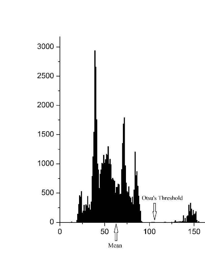
Figure 2: Comparison of mean point and Otsu’s thresholds

3 Experimental Results

The experiments were performed on $24$ commonly used data sets from the UCI Machine Learning Repository [53]. Table 1 gives the data set descriptions. For each data set, the number of clusters ($K$) was set equal to the number of classes ($K^{\prime}$), as commonly seen in the related literature [23, 39, 40, 29, 30, 31, 32, 54].

In clustering applications, normalization is a common preprocessing step that is necessary to prevent attributes with large ranges from dominating the distance calculations and also to avoid numerical instabilities in the computations. Two commonly used normalization schemes are linear scaling to unit range (min-max normalization) and linear scaling to unit variance (z-score normalization). Several studies revealed that the former scheme is preferable to the latter since the latter is likely to eliminate valuable between-cluster variation [55, 40]. As a result, we used min-max normalization to map the attributes of each data set to the $[0,1]$ interval.

Table 1: Data Set Descriptions ($N$: # points, $D$: # attributes, $K^{\prime}$: # classes)

ID	Data Set	$N$	$D$	$K^{\prime}$
1	Abalone	4,177	7	28
2	Breast Cancer Wisconsin (Original)	683	9	2
3	Breast Tissue	106	9	6
4	Ecoli	336	7	8
5	Glass Identification	214	9	6
6	Heart Disease	297	13	5
7	Ionosphere	351	34	2
8	Iris (Bezdek)	150	4	3
9	ISOLET	7,797	617	26
10	Landsat Satellite (Statlog)	6,435	36	6
11	Letter Recognition	20,000	16	26
12	MAGIC Gamma Telescope	19,020	10	2
13	Multiple Features (Fourier)	2,000	76	10
14	Musk (Clean2)	6,598	166	2
15	Optical Digits	5,620	64	10
16	Page Blocks Classification	5,473	10	5
17	Pima Indians Diabetes	768	8	2
18	Shuttle (Statlog)	58,000	9	7
19	Spambase	4,601	57	2
20	SPECTF Heart	267	44	2
21	Wall-Following Robot Navigation	5,456	24	4
22	Wine Quality	6,497	11	7
23	Wine	178	13	3
24	Yeast	1,484	8	10

The performance of the IMs was quantified using two effectiveness (quality) and two efficiency (speed) criteria:

• Initial SSE: This is the SSE value calculated after the initialization phase, before the clustering phase. It gives us a measure of the effectiveness of an IM by itself.

• Final SSE: This is the SSE value calculated after the clustering phase. It gives us a measure of the effectiveness of an IM when its output is refined by k-means. Note that this is the objective function of the k-means algorithm, i.e., (1).

• Number of Iterations: This is the number of iterations that k-means requires until reaching convergence when initialized by a particular IM. It is an efficiency measure independent of programming language, implementation style, compiler, and CPU architecture.

• CPU Time: This is the total CPU time in milliseconds taken by the initialization and clustering phases.

All of the methods were implemented in the C language, compiled with the gcc v4.4.3 compiler, and executed on an Intel Xeon E5520 2.26GHz machine. Time measurements were performed using the getrusage function, which is capable of measuring CPU time to an accuracy of a microsecond. The MT19937 variant of the Mersenne Twister algorithm was used to generate high quality pseudorandom numbers [56].

The convergence of k-means was controlled by the disjunction of two criteria: the number of iterations reaches a maximum of $100$ or the relative improvement in SSE between two consecutive iterations drops below a threshold, i.e., ${{\left({\mbox{SSE}_{i-1}-\mbox{SSE}_{i}}\right)}\mathord{\left/{\vphantom{{\left({\mbox{SSE}_{i-1}-\mbox{SSE}_{i}}\right)}{\mbox{SSE}_{i}}}}\right.\kern-1.2pt}{\mbox{SSE}_{i}}}\leq\varepsilon$, where $\mbox{SSE}_{i}$ denotes the SSE value at the end of the $i$-th ($i\in\{1,2,\dotsc,100\}$) iteration. The convergence threshold was set to $\varepsilon=10^{-6}$.

In this study, we focus on IMs that have time complexity linear in $N$. This is because k-means itself has linear complexity, which is perhaps the most important reason for its popularity. Therefore, an IM for k-means should not diminish this advantage of the algorithm. The proposed methods, named Otsu Var-Part (OV) and Otsu PCA-Part (OP), were compared to six popular, linear, order-invariant IMs: Forgy’s method (F), MacQueen’s second method (M), maximin (X), k-means++ (K), Var-Part (V), and PCA-Part (P). It should be noted that among these methods F, M, and K are random, whereas X, V, P, OV, and OP are deterministic.

We first examine the influence of $L$ (number of histogram bins) on the performance of OV and OP. Tables 2 and 3 show the initial and final SSE values obtained by respectively OV and OP for $L=64,128,256,512,1024$ on four of the largest data sets (the best values are underlined). It can be seen that the performances of both methods are relatively insensitive to the value of $L$. Therefore, in the subsequent experiments we report the results for $L=256$.

Table 2: Influence of $L$ on the effectiveness of Otsu Var-Part ($L$: # histogram bins)

ID	Criterion	$L=64$	$L=128$	$L=256$	$L=512$	$L=1024$
9	Initial SSE	143859	144651	144658	144637	144638
	Final SSE	118267	119127	118033	118033	118034
10	Initial SSE	1987	1920	1919	1920	1920
	Final SSE	1742	1742	1742	1742	1742
11	Initial SSE	3242	3192	3231	3202	3202
	Final SSE	2742	2734	2734	2734	2734
15	Initial SSE	17448	17504	17504	17504	17504
	Final SSE	14581	14581	14581	14581	14581

Table 3: Influence of $L$ on the effectiveness of Otsu PCA-Part ($L$: # histogram bins)

ID	Criterion	$L=64$	$L=128$	$L=256$	$L=512$	$L=1024$
9	Initial SSE	123527	123095	122528	123129	123342
	Final SSE	118575	118577	119326	118298	118616
10	Initial SSE	1855	1807	1835	1849	1848
	Final SSE	1742	1742	1742	1742	1742
11	Initial SSE	2994	2997	2995	2995	2991
	Final SSE	2747	2747	2747	2747	2747
15	Initial SSE	15136	15117	15118	15116	15117
	Final SSE	14650	14650	14650	14650	14650

In the remaining experiments, each random method was executed a $100$ times and statistics such as minimum, mean, and standard deviation were collected for each performance criteria. The minimum and mean statistics represent the best and average case performance, respectively, while standard deviation quantifies the variability of performance across different runs. Note that for a deterministic method, the minimum and mean values are always identical and the standard deviation is always $0$.

Tables Deterministic Initialization of the K-Means Algorithm Using Hierarchical Clustering–Deterministic Initialization of the K-Means Algorithm Using Hierarchical Clustering give the performance measurements for each method with respect to initial SSE, final SSE, number of iterations, and CPU time, respectively. For each of the initial SSE, final SSE, and number of iterations criteria, we calculated the ratio of the minimum/mean/standard deviation value obtained by each method to the best (least) minimum/mean/standard deviation value on each data set. These ratios will be henceforth referred to as the ‘normalized’ performance criteria. For example, on the Abalone data set (1), the minimum initial SSE of F is $424.92$ and the best minimum initial SSE is $21.57$ and thus the normalized initial SSE is about $20$. This simply means that on this data set F obtained approximately $20$ times worse minimum initial SSE than the best method. We then averaged these normalized values over the $24$ data sets to quantify the overall performance of each method with respect to each statistic (see Table 4). Note that we did not attempt to summarize the CPU time values in the same manner due to the sparsity of the data (see Table Deterministic Initialization of the K-Means Algorithm Using Hierarchical Clustering). For convenient visualization, Figure 3 shows box plots of the normalized performance criteria. Here, the bottom and top end of the whiskers of a box represent the minimum and maximum, respectively, whereas the bottom and top of the box itself are the $25$th percentile (Q1) and $75$th percentile (Q3), respectively. The line that passes through the box is the $50$th percentile (Q2), i.e., the median, while the small square inside the box denotes the mean.

4 Discussion

4.1 Best Case Performance Analysis

With respect to the minimum statistic, the following observations can be made:

• Initial SSE: OP is the best method, followed closely by P, OV, and V. On the other hand, F is the worst method, followed by X. These two methods give $2$–$3$ times worse minimum initial SSE than the best method. It can be seen that multiple runs of random methods do not produce good initial clusterings. In contrast, only a single run of OP, P, OV, or V often gives very good results. This is because these methods are approximate clustering algorithms by themselves and thus they give reasonable results even without k-means refinement.

• Final SSE: X is the worst method, while the remaining methods exhibit very similar performance. This homogeneity in performance is because k-means can take two disparate initial configurations to similar (or even identical) local minima. Given the abundance of local minima even in data sets of moderate size and/or dimensionality and the gradient descent nature of k-means, it is not surprising that the deterministic methods (except X) perform slightly worse than the random methods as the former methods were executed only once, whereas the latter ones were executed a $100$ times.

• Number of Iterations: K is the best method, followed by M and F. X is the worst method. As in the case of final SSE, random methods outperform deterministic methods due to their multiple-run advantage.

4.2 Average Case Performance Analysis

With respect to the mean statistic, the following observations can be made:

• Initial SSE: OP is the best method, followed closely by P, OV, and V. The remaining methods give $1.7$–$3.2$ times worse mean initial SSE than any of these hierarchical methods. Random methods exhibit significantly worse average performance than the deterministic ones because the former methods can produce highly variable results across different runs (see the standard deviation values in Table Deterministic Initialization of the K-Means Algorithm Using Hierarchical Clustering).

• Final SSE: This is similar to the case of minimum final SSE, with the difference that deterministic methods (except X) are now slightly better than the random ones. Once again, this is because random methods can produce highly variable results due to their stochastic nature.

• Number of Iterations: The ranking of the methods is similar to the case of mean final SSE.

4.3 Consistency Analysis

With respect to the standard deviation statistic, F is significantly better than both M and K. If, however, the application requires absolute consistency, i.e., exactly the same clustering in every run, a deterministic IM should be used.

4.4 CPU Time Analysis

It can be seen from Table Deterministic Initialization of the K-Means Algorithm Using Hierarchical Clustering that, on about half of the data sets, each of the IMs require less than a few milliseconds of CPU time. On the other hand, on large and/or high-dimensional data sets efficiency differences become more prominent. It should be noted that each of the values reported in this table corresponds to a single k-means ‘run’. In practice, a random method is typically executed $R$ times, e.g., in this study $R=100$, and the output of the run that gives the least final SSE is taken as the result. Therefore, the total computational cost of a random method is often significantly higher than that of a deterministic method. For example, on the ISOLET data set, which has the greatest $N\times D\times K$ value among all the data sets, K took on the average $3,397$ milliseconds, whereas OP took $12,460$ milliseconds. The latter method, however, required about $27$ times less CPU time than the former one since the former was executed a total of $100$ times.

4.5 Relative Performance Analysis

We also determined the number of data sets (out of 24) on which OV and OP respectively performed $\{$worse than/same as/better than$\}$ V and P. Tables 5 and 6 present the results for OV and OP, respectively. It can be seen that, with respect to initial SSE and number of iterations criteria, OV outperforms V more often than not. On the other hand, OP frequently outperforms P with respect to both criteria. As for final SSE, OP performs slightly better than P, whereas OV performs slightly worse than V. It appears that Otsu’s method benefits P more than it benefits V. This is most likely due to the fact that histograms of projections over the major axis necessarily have a greater dynamic range and variability and thus are more amenable to thresholding compared to histograms of projections over any coordinate axis.

4.6 Recommendations for Practitioners

Based on the analyses presented above, the following recommendations can be made:

• In general, X should not be used. As mentioned in Section 2, this method was not designed specifically as a k-means initializer [43]. It is easy to understand and implement, but is mostly ineffective and unreliable. Furthermore, despite its low overhead, this method does not offer significant time savings since it often results in slow k-means convergence.

• In applications that involve small data sets, e.g., $N<1,000$, K should be used. It is computationally feasible to run this method hundreds of times on such data sets given that one such run takes only a few milliseconds.

• In time-critical applications that involve large data sets or applications that demand determinism, the hierarchical methods should be used. These methods need to be executed only once and they lead to reasonably fast k-means convergence. The efficiency difference between V/OV and P/OP is noticeable only on high dimensional data sets such as ISOLET ($D=617$) and Musk ($D=166$). This is because V/OV calculates the direction of split by determining the coordinate axis with the greatest variance (in $\mathcal{O}(D)$ time), whereas P/OP achieves this by calculating the principal eigenvector of the cluster covariance matrix (in $\mathcal{O}(D^{2})$ time using the power method [44]). Note that despite its higher computational complexity, P/OP can, in some cases, be more efficient than V/OV (see Table Deterministic Initialization of the K-Means Algorithm Using Hierarchical Clustering). This is because the former converges significantly faster than the latter (see Table 4). The main disadvantage of these methods is that they are more complicated to implement due to their hierarchical formulation.

• In applications where an approximate clustering of the data set is desired, the hierarchical methods should be used. These methods produce very good initial clusterings, which makes it possible to use them as standalone clustering algorithms.

• Among the hierarchical methods, the ones based on PCA, i.e., P and OP, are preferable to those based on variance, i.e., V and OV. Furthermore, the proposed OP and OV methods generally outperform their respective counterparts, i.e., P and V, especially with respect to initial SSE and number of iterations.

5 Conclusions

In this paper, we presented a simple modification to Var-Part and PCA-Part, two hierarchical k-means initialization methods that are linear, deterministic, and order-invariant. We compared the original methods and their modified versions to some of the most popular linear initialization methods, namely Forgy’s method, Macqueen’s second method, maximin, and k-means++, on a large and diverse collection of data sets from the UCI Machine Learning Repository. The results demonstrated that, despite their deterministic nature, Var-Part and PCA-Part are highly competitive with one of the best random initialization methods to date, i.e., k-means++. In addition, the proposed modification significantly improves the performance of both hierarchical methods. The presented Var-Part and PCA-Part variants can be used to initialize k-means effectively, particularly in time-critical applications that involve large data sets. Alternatively, they can be used as approximate clustering algorithms without additional k-means refinement.

6 Acknowledgments

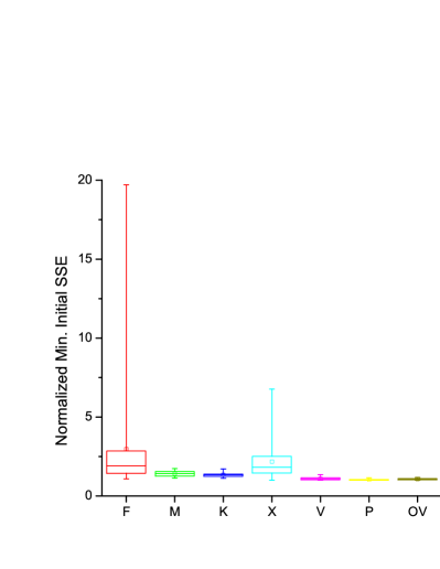
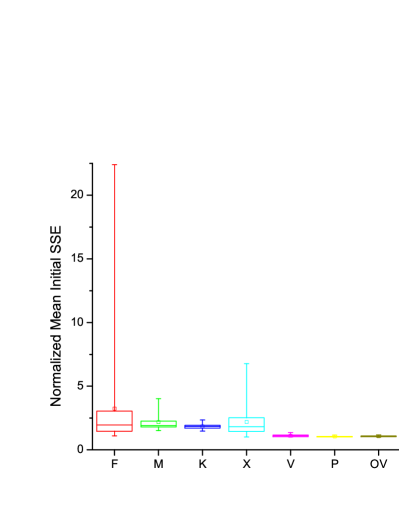
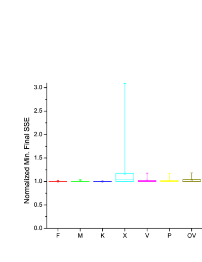
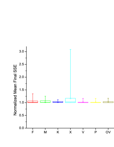
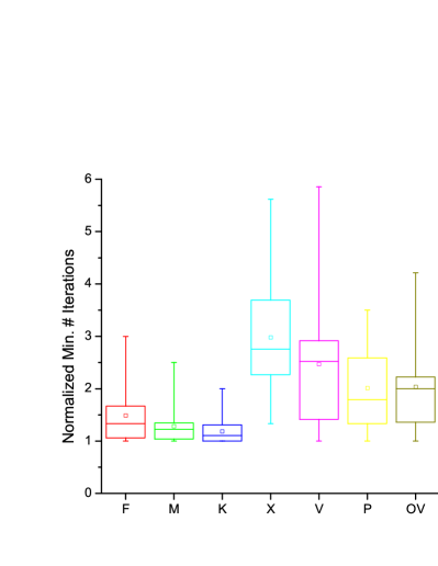
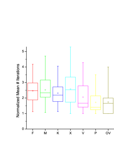
This publication was made possible by grants from the Louisiana Board of Regents (LEQSF2008-11-RD-A-12) and National Science Foundation (0959583, 1117457).

References

- [1] A. K. Jain, M. N. Murty, and P. J. Flynn, “Data Clustering: A Review,” ACM Computing Surveys, vol. 31, no. 3, pp. 264–323, 1999.
- [2] A. K. Jain, “Data Clustering: 50 Years Beyond K-Means,” Pattern Recognition Letters, vol. 31, no. 8, pp. 651–666, 2010.
- [3] L. Kaufman and P. Rousseeuw, Finding Groups in Data: An Introduction to Cluster Analysis. Wiley-Interscience, 1990.
- [4] D. Aloise, A. Deshpande, P. Hansen, and P. Popat, “NP-Hardness of Euclidean Sum-of-Squares Clustering,” Machine Learning, vol. 75, no. 2, pp. 245–248, 2009.
- [5] M. Mahajan, P. Nimbhorkar, and K. Varadarajan, “The Planar k-Means Problem is NP-hard,” Theoretical Computer Science, vol. 442, pp. 13–21, 2012.
- [6] A. Tarsitano, “A Computational Study of Several Relocation Methods for K-Means Algorithms,” Pattern Recognition, vol. 36, no. 12, pp. 2955–2966, 2003.
- [7] S. Lloyd, “Least Squares Quantization in PCM,” IEEE Transactions on Information Theory, vol. 28, no. 2, pp. 129–136, 1982.
- [8] P. S. Bradley and U. Fayyad, “Refining Initial Points for K-Means Clustering,” in Proc. of the 15th Int. Conf. on Machine Learning, pp. 91–99, 1998.
- [9] M. Dash, H. Liu, and X. Xu, “’’: Merging Distance and Density Based Clustering,” in Proc. of the 7th Int. Conf. on Database Systems for Advanced Applications, pp. 32–39, 2001.
- [10] W. Y. Chen, Y. Song, H. Bai, C. J. Lin, and E. Y. Chang, “Parallel Spectral Clustering in Distributed Systems,” IEEE Transactions on Pattern Analysis and Machine Intelligence, vol. 33, no. 3, pp. 568–586, 2011.
- [11] T. Kanungo, D. Mount, N. Netanyahu, C. Piatko, R. Silverman, and A. Wu, “An Efficient K-Means Clustering Algorithm: Analysis and Implementation,” IEEE Transactions on Pattern Analysis and Machine Intelligence, vol. 24, no. 7, pp. 881–892, 2002.
- [12] G. Hamerly, “Making k-means Even Faster,” in Proc. of the 2010 SIAM Int. Conf. on Data Mining, pp. 130–140, 2010.
- [13] T. W. Chen and S. Y. Chien, “Bandwidth Adaptive Hardware Architecture of K-Means Clustering for Video Analysis,” IEEE Transactions on Very Large Scale Integration (VLSI) Systems, vol. 18, no. 6, pp. 957–966, 2010.
- [14] C. Ordonez and E. Omiecinski, “Efficient Disk-Based K-Means Clustering for Relational Databases,” IEEE Transactions on Knowledge and Data Engineering, vol. 16, no. 8, pp. 909–921, 2004.
- [15] S. Z. Selim and M. A. Ismail, “K-Means-Type Algorithms: A Generalized Convergence Theorem and Characterization of Local Optimality,” IEEE Transactions on Pattern Analysis and Machine Intelligence, vol. 6, no. 1, pp. 81–87, 1984.
- [16] L. Bottou and Y. Bengio, “Convergence Properties of the K-Means Algorithms,” in Advances in Neural Information Processing Systems 7 (G. Tesauro, D. S. Touretzky, and T. K. Leen, eds.), pp. 585–592, MIT Press, 1995.
- [17] L. Vendramin, R. J. G. B. Campello, and E. R. Hruschka, “Relative Clustering Validity Criteria: A Comparative Overview,” Statistical Analysis and Data Mining, vol. 3, no. 4, pp. 209–235, 2010.
- [18] J. Mao and A. K. Jain, “A Self-Organizing Network for Hyperellipsoidal Clustering (HEC),” IEEE Transactions on Neural Networks, vol. 7, no. 1, pp. 16–29, 1996.
- [19] J. S. Zhang and Y.-W. Leung, “Robust Clustering by Pruning Outliers,” IEEE Transactions on Systems, Man, and Cybernetics – Part B, vol. 33, no. 6, pp. 983–999, 2003.
- [20] M. E. Celebi, H. Kingravi, and P. A. Vela, “A Comparative Study of Efficient Initialization Methods for the K-Means Clustering Algorithm,” Expert Systems with Applications, vol. 40, no. 1, pp. 200–210, 2013.
- [21] M. E. Celebi, “Improving the Performance of K-Means for Color Quantization,” Image and Vision Computing, vol. 29, no. 4, pp. 260–271, 2011.
- [22] J. M. Pena, J. A. Lozano, and P. Larranaga, “An Empirical Comparison of Four Initialization Methods for the K-Means Algorithm,” Pattern Recognition Letters, vol. 20, no. 10, pp. 1027–1040, 1999.
- [23] J. He, M. Lan, C. L. Tan, S. Y. Sung, and H. B. Low, “Initialization of Cluster Refinement Algorithms: A Review and Comparative Study,” in Proc. of the 2004 IEEE Int. Joint Conf. on Neural Networks, pp. 297–302, 2004.
- [24] G. N. Lance and W. T. Williams, “A General Theory of Classificatory Sorting Strategies - II. Clustering Systems,” The Computer Journal, vol. 10, no. 3, pp. 271–277, 1967.
- [25] M. M. Astrahan, “Speech Analysis by Clustering, or the Hyperphoneme Method,” Tech. Rep. AIM-124, Stanford University, 1970.
- [26] J. A. Hartigan and M. A. Wong, “Algorithm AS 136: A K-Means Clustering Algorithm,” Journal of the Royal Statistical Society C, vol. 28, no. 1, pp. 100–108, 1979.
- [27] A. Likas, N. Vlassis, and J. Verbeek, “The Global K-Means Clustering Algorithm,” Pattern Recognition, vol. 36, no. 2, pp. 451–461, 2003.
- [28] M. Al-Daoud, “A New Algorithm for Cluster Initialization,” in Proc. of the 2nd World Enformatika Conf., pp. 74–76, 2005.
- [29] S. J. Redmond and C. Heneghan, “A Method for Initialising the K-Means Clustering Algorithm Using kd-trees,” Pattern Recognition Letters, vol. 28, no. 8, pp. 965–973, 2007.
- [30] M. Al Hasan, V. Chaoji, S. Salem, and M. Zaki, “Robust Partitional Clustering by Outlier and Density Insensitive Seeding,” Pattern Recognition Letters, vol. 30, no. 11, pp. 994–1002, 2009.
- [31] F. Cao, J. Liang, and G. Jiang, “An Initialization Method for the K-Means Algorithm Using Neighborhood Model,” Computers and Mathematics with Applications, vol. 58, no. 3, pp. 474–483, 2009.
- [32] P. Kang and S. Cho, “K-Means Clustering Seeds Initialization Based on Centrality, Sparsity, and Isotropy,” in Proc. of the 10th Int. Conf. on Intelligent Data Engineering and Automated Learning, pp. 109–117, 2009.
- [33] E. Forgy, “Cluster Analysis of Multivariate Data: Efficiency vs. Interpretability of Classification,” Biometrics, vol. 21, p. 768, 1965.
- [34] R. C. Jancey, “Multidimensional Group Analysis,” Australian Journal of Botany, vol. 14, no. 1, pp. 127–130, 1966.
- [35] J. MacQueen, “Some Methods for Classification and Analysis of Multivariate Observations,” in Proc. of the 5th Berkeley Symposium on Mathematical Statistics and Probability, pp. 281–297, 1967.
- [36] G. H. Ball and D. J. Hall, “A Clustering Technique for Summarizing Multivariate Data,” Behavioral Science, vol. 12, no. 2, pp. 153–155, 1967.
- [37] J. T. Tou and R. C. Gonzales, Pattern Recognition Principles. Addison-Wesley, 1974.
- [38] H. Späth, “Computational Experiences with the Exchange Method: Applied to Four Commonly Used Partitioning Cluster Analysis Criteria,” European Journal of Operational Research, vol. 1, no. 1, pp. 23–31, 1977.
- [39] D. Arthur and S. Vassilvitskii, “k-means++: The Advantages of Careful Seeding,” in Proc. of the 18th Annual ACM-SIAM Symposium on Discrete Algorithms, pp. 1027–1035, 2007.
- [40] T. Su and J. G. Dy, “In Search of Deterministic Methods for Initializing K-Means and Gaussian Mixture Clustering,” Intelligent Data Analysis, vol. 11, no. 4, pp. 319–338, 2007.
- [41] M. R. Anderberg, Cluster Analysis for Applications. Academic Press, 1973.
- [42] M. J. Norušis, IBM SPSS Statistics 19 Statistical Procedures Companion. Addison Wesley, 2011.
- [43] T. Gonzalez, “Clustering to Minimize the Maximum Intercluster Distance,” Theoretical Computer Science, vol. 38, no. 2–3, pp. 293–306, 1985.
- [44] H. Hotelling, “Simplified Calculation of Principal Components,” Psychometrika, vol. 1, no. 1, pp. 27–35, 1936.
- [45] E. H. Ruspini, “Numerical Methods for Fuzzy Clustering,” Information Sciences, vol. 2, no. 3, pp. 319–350, 1970.
- [46] M. Sezgin and B. Sankur, “Survey over Image Thresholding Techniques and Quantitative Performance Evaluation,” Journal of Electronic Imaging, vol. 13, no. 1, pp. 146–165, 2004.
- [47] N. Otsu, “A Threshold Selection Method from Gray Level Histograms,” IEEE Transactions on Systems, Man and Cybernetics, vol. 9, no. 1, pp. 62–66, 1979.
- [48] P. K. Sahoo, S. Soltani, and A. K. C. Wong, “A Survey of Thresholding Techniques,” Computer Vision, Graphics, and Image Processing, vol. 41, no. 2, pp. 233–260, 1988.
- [49] S. U. Lee, S. Y. Chung, and R. H. Park, “A Comparative Performance Study of Several Global Thresholding Techniques,” Computer Vision, Graphics, and Image Processing, vol. 52, no. 2, pp. 171–190, 1990.
- [50] O. D. Trier and T. Taxt, “Evaluation of Binarization Methods for Document Images,” IEEE Transactions on Pattern Analysis and Machine Intelligence, vol. 17, no. 3, pp. 312–315, 1995.
- [51] R. Medina-Carnicer, F. J. Madrid-Cuevas, N. L. Fernandez-Garcia, and A. Carmona-Poyato, “Evaluation of Global Thresholding Techniques in Non-Contextual Edge Detection,” Pattern Recognition Letters, vol. 26, no. 10, pp. 1423–1434, 2005.
- [52] M. E. Celebi, Q. Wen, S. Hwang, H. Iyatomi, and G. Schaefer, “Lesion Border Detection in Dermoscopy Images Using Ensembles of Thresholding Methods,” Skin Research and Technology, vol. 19, no. 1, pp. e252–e258, 2013.
- [53] A. Frank and A. Asuncion, “UCI Machine Learning Repository.” http://archive.ics.uci.edu/ml, 2012. University of California, Irvine, School of Information and Computer Sciences.
- [54] T. Onoda, M. Sakai, and S. Yamada, “Careful Seeding Method based on Independent Components Analysis for k-means Clustering,” Journal of Emerging Technologies in Web Intelligence, vol. 4, no. 1, pp. 51–59, 2012.
- [55] G. Milligan and M. C. Cooper, “A Study of Standardization of Variables in Cluster Analysis,” Journal of Classification, vol. 5, no. 2, pp. 181–204, 1988.
- [56] M. Matsumoto and T. Nishimura, “Mersenne Twister: A 623-Dimensionally Equidistributed Uniform Pseudo-Random Number Generator,” ACM Transactions on Modeling and Computer Simulation, vol. 8, no. 1, pp. 3–30, 1998.
Initial SSE comparison of the initialization methods
{xtabular}c—c—r—r—r—r—r—r—r—r
F M K X V P OV OP
1 min 425 33 29 95 24 23 23 22
mean 483 20 46 10 34 2 95 0 24 0 23 0 23 0 22 0
2 min 534 318 304 498 247 240 258 239
mean 575 15 706 354 560 349 498 0 247 0 240 0 258 0 239 0
3 min 20 11 9 19 8 8 8 7
mean 27 3 20 8 13 2 19 0 8 0 8 0 8 0 7 0
4 min 54 26 26 48 20 19 19 20
mean 61 2 40 7 33 5 48 0 20 0 19 0 19 0 20 0
5 min 42 24 25 45 21 20 21 18
mean 48 2 40 9 32 5 45 0 21 0 20 0 21 0 18 0
6 min 372 361 341 409 249 250 249 244
mean 396 8 463 58 450 49 409 0 249 0 250 0 249 0 244 0
7 min 771 749 720 827 632 629 636 629
mean 814 12 1246 463 1237 468 827 0 632 0 629 0 636 0 629 0
8 min 26 9 9 18 8 8 7 7
mean 34 4 28 23 16 6 18 0 8 0 8 0 7 0 7 0
9 min 218965 212238 210387 221163 145444 124958 144658 122528
mean 223003 1406 224579 5416 223177 4953 221163 0 145444 0 124958 0 144658 0 122528 0
10 min 7763 2637 2458 4816 2050 2116 1919 1835
mean 8057 98 4825 1432 3561 747 4816 0 2050 0 2116 0 1919 0 1835 0
11 min 7100 4203 4158 5632 3456 3101 3231 2995
mean 7225 30 4532 165 4501 176 5632 0 3456 0 3101 0 3231 0 2995 0
12 min 4343 3348 3296 4361 3056 2927 3060 2923
mean 4392 13 5525 1816 5346 1672 4361 0 3056 0 2927 0 3060 0 2923 0
13 min 4416 5205 5247 4485 3354 3266 3315 3180
mean 4475 25 5693 315 5758 283 4485 0 3354 0 3266 0 3315 0 3180 0
14 min 53508 56841 56822 54629 37334 37142 37282 36375
mean 54312 244 82411 14943 75532 12276 54629 0 37334 0 37142 0 37282 0 36375 0
15 min 25466 25492 24404 25291 17476 15714 17504 15118
mean 25811 99 28596 1550 27614 1499 25291 0 17476 0 15714 0 17504 0 15118 0
16 min 633 275 250 635 300 230 232 222
mean 648 6 423 74 372 72 635 0 300 0 230 0 232 0 222 0
17 min 152 144 141 156 124 122 123 121
mean 156 1 216 44 219 61 156 0 124 0 122 0 123 0 121 0
18 min 1788 438 328 1818 316 309 276 268
mean 1806 6 946 290 494 115 1818 0 316 0 309 0 276 0 268 0
19 min 834 873 881 772 782 783 792 765
mean 838 1 1186 386 1124 244 772 0 782 0 783 0 792 0 765 0
20 min 269 295 297 277 232 222 225 214
mean 281 4 384 88 413 159 277 0 232 0 222 0 225 0 214 0
21 min 10976 11834 11829 11004 8517 7805 8706 7802
mean 11082 34 14814 1496 14435 1276 11004 0 8517 0 7805 0 8706 0 7802 0
22 min 719 473 449 733 386 361 364 351
mean 729 4 601 59 567 64 733 0 386 0 361 0 364 0 351 0
23 min 78 76 70 87 51 53 50 51
mean 87 3 113 22 101 20 87 0 51 0 53 0 50 0 51 0
24 min 144 89 83 115 77 63 73 63
mean 149 2 110 8 101 9 115 0 77 0 63 0 73 0 63 0
Final SSE comparison of the initialization methods
{xtabular}c—c—r—r—r—r—r—r—r—r
F M K X V P OV OP
1 min 21 22 21 25 21 21 21 21
mean 23 1 22 1 22 0 25 0 21 0 21 0 21 0 21 0
2
min 239 239 239 239 239 239 239 239
mean 239 0 239 0 239 0 239 0 239 0 239 0 239 0 239 0
3
min 7 7 7 7 7 7 8 7
mean 8 1 9 1 8 1 7 0 7 0 7 0 8 0 7 0
4
min 17 17 17 19 17 18 18 18
mean 19 1 19 2 19 1 19 0 17 0 18 0 18 0 18 0
5
min 18 18 18 23 19 19 20 18
mean 20 1 21 2 20 2 23 0 19 0 19 0 20 0 18 0
6
min 243 243 243 249 248 243 248 243
mean 252 8 252 8 252 8 249 0 248 0 243 0 248 0 243 0
7
min 629 629 629 826 629 629 629 629
mean 629 0 643 50 641 47 826 0 629 0 629 0 629 0 629 0
8
min 7 7 7 7 7 7 7 7
mean 8 1 8 2 7 1 7 0 7 0 7 0 7 0 7 0
9
min 117872 117764 117710 135818 118495 118386 118033 119326
mean 119650 945 119625 947 119536 934 135818 0 118495 0 118386 0 118033 0 119326 0
10
min 1742 1742 1742 1742 1742 1742 1742 1742
mean 1742 0 1742 0 1744 28 1742 0 1742 0 1742 0 1742 0 1742 0
11
min 2723 2718 2716 2749 2735 2745 2734 2747
mean 2772 29 2757 19 2751 19 2749 0 2735 0 2745 0 2734 0 2747 0
12
min 2923 2923 2923 2923 2923 2923 2923 2923
mean 2923 0 2923 0 2923 0 2923 0 2923 0 2923 0 2923 0 2923 0
13
min 3127 3128 3128 3316 3137 3214 3143 3153
mean 3166 31 3172 29 3173 35 3316 0 3137 0 3214 0 3143 0 3153 0
14
min 36373 36373 36373 36373 36373 36373 36373 36373
mean 37296 1902 37163 1338 37058 1626 36373 0 36373 0 36373 0 36373 0 36373 0
15
min 14559 14559 14559 14679 14581 14807 14581 14650
mean 14687 216 14752 236 14747 245 14679 0 14581 0 14807 0 14581 0 14650 0
16
min 215 215 215 230 227 215 229 216
mean 217 4 216 2 220 7 230 0 227 0 215 0 229 0 216 0
17
min 121 121 121 121 121 121 121 121
mean 121 0 122 5 122 5 121 0 121 0 121 0 121 0 121 0
18
min 235 235 235 726 235 274 274 235
mean 317 46 272 23 260 31 726 0 235 0 274 0 274 0 235 0
19
min 765 765 765 765 778 778 778 765
mean 778 3 779 14 785 19 765 0 778 0 778 0 778 0 765 0
20
min 214 214 214 214 214 214 214 214
mean 214 0 215 5 214 0 214 0 214 0 214 0 214 0 214 0
21
min 7772 7772 7772 7772 7774 7774 7774 7772
mean 7799 93 7821 124 7831 140 7772 0 7774 0 7774 0 7774 0 7772 0
22
min 334 334 334 399 335 334 335 335
mean 335 1 336 3 336 3 399 0 335 0 334 0 335 0 335 0
23
min 49 49 49 63 49 49 49 49
mean 49 0 49 2 49 2 63 0 49 0 49 0 49 0 49 0
24
min 58 58 58 61 69 59 69 59
mean 64 6 69 6 63 5 61 0 69 0 59 0 69 0 59 0
\tablecaptionNumber of iterations comparison of the initialization methods
{xtabular}c—c—r—r—r—r—r—r—r—r
F M K X V P OV OP
1 min 59 29 22 100 50 43 31 38
mean 90 11 68 19 48 17 100 0 50 0 43 0 31 0 38 0
2
min 4 4 4 8 4 4 5 3
mean 5 0 6 1 6 1 8 0 4 0 4 0 5 0 3 0
3
min 5 5 3 7 6 7 5 3
mean 10 2 9 3 7 2 7 0 6 0 7 0 5 0 3 0
4
min 8 6 7 14 17 7 12 6
mean 15 6 15 5 14 5 14 0 17 0 7 0 12 0 6 0
5
min 6 5 4 6 6 5 9 4
mean 10 3 11 4 9 3 6 0 6 0 5 0 9 0 4 0
6
min 5 5 5 12 3 4 3 4
mean 11 3 10 3 9 3 12 0 3 0 4 0 3 0 4 0
7
min 4 3 3 3 3 3 4 2
mean 5 1 7 2 8 2 3 0 3 0 3 0 4 0 2 0
8
min 4 4 3 6 4 4 6 3
mean 9 3 8 2 7 3 6 0 4 0 4 0 6 0 3 0
9
min 18 19 14 32 82 45 59 39
mean 43 15 40 14 36 13 32 0 82 0 45 0 59 0 39 0
10
min 12 12 11 53 28 27 10 23
mean 28 8 33 10 29 9 53 0 28 0 27 0 10 0 23 0
11
min 39 37 31 73 100 83 67 85
mean 75 19 72 18 76 18 73 0 100 0 83 0 67 0 85 0
12
min 9 10 10 35 25 10 26 9
mean 18 5 18 5 20 6 35 0 25 0 10 0 26 0 9 0
13
min 13 14 13 37 14 25 17 13
mean 29 10 30 10 30 11 37 0 14 0 25 0 17 0 13 0
14
min 4 4 4 8 5 5 5 3
mean 6 1 6 1 6 1 8 0 5 0 5 0 5 0 3 0
15
min 12 12 14 36 16 22 15 59
mean 31 13 33 14 30 10 36 0 16 0 22 0 15 0 59 0
16
min 14 12 9 27 25 15 19 16
mean 27 9 31 14 24 11 27 0 25 0 15 0 19 0 16 0
17
min 8 4 4 19 11 10 8 5
mean 13 2 12 5 11 4 19 0 11 0 10 0 8 0 5 0
18
min 10 8 9 22 30 16 7 27
mean 25 9 25 11 23 9 22 0 30 0 16 0 7 0 27 0
19
min 6 3 3 5 9 10 12 3
mean 12 5 14 6 12 7 5 0 9 0 10 0 12 0 3 0
20
min 6 5 4 7 7 7 6 2
mean 8 1 8 2 7 2 7 0 7 0 7 0 6 0 2 0
21
min 9 11 11 24 20 8 21 19
mean 20 8 22 8 20 8 24 0 20 0 8 0 21 0 19 0
22
min 15 17 18 20 62 50 33 49
mean 41 20 42 18 40 18 20 0 62 0 50 0 33 0 49 0
23
min 4 4 4 9 5 7 5 5
mean 7 2 8 3 7 3 9 0 5 0 7 0 5 0 5 0
24
min 13 13 15 73 33 21 28 32
mean 29 10 31 11 29 10 73 0 33 0 21 0 28 0 32 0
\tablecaptionCPU time comparison of the initialization methods
{xtabular}c—c—r—r—r—r—r—r—r—r
F M K X V P OV OP
1 min 20 10 10 40 20 20 20 10
mean 43 7 33 10 24 9 40 0 20 0 20 0 20 0 10 0
2
min 0 0 0 0 0 0 0 0
mean 0 1 0 1 0 2 0 0 0 0 0 0 0 0 0 0
3
min 0 0 0 0 0 0 0 0
mean 0 1 0 1 0 0 0 0 0 0 0 0 0 0 0 0
4
min 0 0 0 0 0 0 0 0
mean 0 2 0 1 0 2 0 0 0 0 0 0 0 0 0 0
5
min 0 0 0 0 0 0 0 0
mean 0 1 0 1 0 1 0 0 0 0 0 0 0 0 0 0
6
min 0 0 0 0 0 0 0 0
mean 0 1 0 2 1 2 0 0 0 0 0 0 0 0 0 0
7
min 0 0 0 0 0 0 0 0
mean 0 2 0 2 0 2 0 0 0 0 0 0 0 0 0 0
8
min 0 0 0 0 0 0 0 0
mean 0 0 0 1 0 1 0 0 0 0 0 0 0 0 0 0
9
min 1690 1630 1580 2570 6920 12160 5040 12460
mean 3691 1229 3370 1178 3397 1055 2570 0 6920 0 12160 0 5040 0 12460 0
10
min 0 10 10 50 30 50 10 50
mean 30 9 32 11 32 10 50 0 30 0 50 0 10 0 50 0
11
min 380 350 320 670 960 790 620 810
mean 710 174 673 168 724 166 670 0 960 0 790 0 620 0 810 0
12
min 10 10 10 40 20 10 30 20
mean 19 7 19 7 21 6 40 0 20 0 10 0 30 0 20 0
13
min 20 20 20 60 20 80 30 40
mean 52 17 52 17 57 20 60 0 20 0 80 0 30 0 40 0
14
min 10 10 10 30 30 210 20 200
mean 22 7 21 5 25 8 30 0 30 0 210 0 20 0 200 0
15
min 50 50 50 140 60 140 70 280
mean 122 50 126 53 124 41 140 0 60 0 140 0 70 0 280 0
16
min 0 0 0 10 10 10 10 10
mean 9 5 11 6 8 5 10 0 10 0 10 0 10 0 10 0
17
min 0 0 0 0 0 0 0 0
mean 0 2 1 2 1 2 0 0 0 0 0 0 0 0 0 0
18
min 40 30 30 50 100 70 30 100
mean 87 27 87 37 79 26 50 0 100 0 70 0 30 0 100 0
19
min 0 0 0 10 10 30 10 20
mean 11 5 12 6 11 8 10 0 10 0 30 0 10 0 20 0
20
min 0 0 0 0 0 0 0 0
mean 0 2 0 2 0 2 0 0 0 0 0 0 0 0 0 0
21
min 10 10 10 20 20 20 20 30
mean 21 9 20 8 20 8 20 0 20 0 20 0 20 0 30 0
22
min 10 20 20 10 60 50 40 40
mean 40 19 40 18 38 17 10 0 60 0 50 0 40 0 40 0
23
min 0 0 0 0 0 0 0 0
mean 0 1 0 1 0 0 0 0 0 0 0 0 0 0 0 0
24
min 0 0 0 10 0 0 10 0
mean 6 5 6 5 6 5 10 0 0 0 0 0 10 0 0 0