Clustering at high redshift: The connection between Lyman Alpha emitters and Lyman break galaxies

Abstract

We present a physically motivated semi-analytic model to understand the clustering of high redshift Lyman-$\alpha$ Emitters (LAEs). We show that the model parameters constrained by the observed luminosity functions, can be used to predict large scale bias and angular correlation function of LAEs. These predictions are shown to reproduce the observations remarkably well. We find that average masses of dark matter halos hosting LAEs brighter than threshold narrow band magnitude $\sim 25$ are $\sim 10^{11}M_{\odot}$. These are smaller than that of typical Lyman Break Galaxies (LBGs) brighter than similar threshold continuum magnitude by a factor $\sim 10$. This results in a smaller clustering strength of LAEs compared to LBGs. However, using the observed relationship between UV continuum and Lyman-$\alpha$ luminosity of LAEs, we show that both LAEs and LBGs belong to the same parent galaxy population with narrow band techniques having greater efficiency in picking up galaxies with low UV luminosity. We also show that the lack of evidence for the presence of the one halo term in the observed LAE angular correlation functions can be attributed to sub-Poisson distribution of LAEs in dark matter halos as a result of their low halo occupations.

1 Introduction

Over the past decade there has been a growing wealth of observations probing the properties of high redshift galaxies (Steidel et al., 1999; Giavalisco et al., 2004; Ouchi et al., 2004a; Beckwith et al., 2006; Grogin et al., 2011; Illingworth et al., 2013). Various surveys, using the Lyman break color selection technique (see for example, Madau et al., 1996; Steidel et al., 1996; Adelberger et al., 1998; Steidel et al., 1998), provided fairly good estimates of luminosity functions (LF) up to $z\sim 8$ (Bouwens et al., 2007, 2008; Reddy et al., 2008; McLure et al., 2012; Schenker et al., 2013; Oesch et al., 2013; Lorenzoni et al., 2013) and spatial clustering up to $z\sim 5$ (Giavalisco & Dickinson, 2001; Ouchi et al., 2004b, 2005; Kashikawa et al., 2006; Hildebrandt et al., 2009; Savoy et al., 2011; Bielby et al., 2011) of these Lyman break galaxies (LBG). On the other hand, narrow-band searches for high redshift Lyman-$\alpha$ line (Hu et al., 1998; Rhoads et al., 2000; Ouchi et al., 2003; Shimasaku et al., 2006a; Gronwall et al., 2007; Finkelstein et al., 2007; Dawson et al., 2007; Ouchi et al., 2008; Shioya et al., 2009; Wang et al., 2009; Hu et al., 2010; Ouchi et al., 2010) have detected substantial number of Lyman-$\alpha$ emitters (LAEs). These surveys helped to infer the statistical properties of LAEs, particularly their UV and Lyman-$\alpha$ luminosity functions and angular correlation functions (Ouchi et al., 2003, 2008; Shioya et al., 2009; Wang et al., 2009; Ouchi et al., 2010). While LBGs selected through colour cuts are biased towards bright galaxies, the narrow band selection of LAEs is biased towards galaxies having strong Lyman-$\alpha$ emission line and weak continuum emission. Therefore, these two techniques pickup galaxies with different type of selection biases. Despite several detailed studies there is no clear consensus on whether there is any differences between the two populations based, on properties such as stellar mass, dust content, age and star formation rate etc (see for example, Gawiser et al., 2006; Pentericci et al., 2007; Ouchi et al., 2008; Kornei et al., 2010a).

In the hierarchical model of structure formation the statistical properties of galaxies are determined by that of the parent dark matter halo population, given a prescription for how stars form inside these halos. The properties of dark matter halos are quite well understood using N-body simulations and analytical models like the halo model of large scale structure. There have been a number of studies over the past years, probing the properties of LAEs using semi-analytical and numerical (simulation) methods (Shimasaku et al., 2006b; Le Delliou et al., 2006; Mao et al., 2007; Kobayashi et al., 2007; Samui et al., 2007; Dayal et al., 2008; Tilvi et al., 2009; Samui et al., 2009; Zheng et al., 2010; Hu et al., 2010; Nagamine et al., 2010; Garel et al., 2012; Forero-Romero et al., 2011; Kobayashi et al., 2010; Dijkstra & Wyithe, 2012). These models have been successful in reproducing the (i) UV LF of LBGs, (ii) UV LF of LAEs and (iii) Lyman-$\alpha$ LF of LAEs. We also have been extensively developing simple physical models of galaxy formation to understand the LFs of LBGs and Lyman-$\alpha$ emitters. Any galaxy formation model that can simultaneously explain the observed properties (like for example, Dayal & Ferrara, 2012) of LBGs and LAEs is very useful to further our understanding of physics of galaxy formation at high-$z$.

In particular by modelling the clustering of LBGs and LAEs one will be able to understand any differences in the range of halo masses probed by these two population of sources. Recently we have presented a physically motivated semi-analytic halo model to simultaneously explain the LF and spatial clustering of high-$z$ LBGs (Jose et al., 2013, hereafter J13). Here we extend this model to explain the measured LFs and angular correlation function of high-$z$ LAEs. The organization of this paper is as follows. In the next section we briefly outline our models for computation of the LF of LAE. In Section 3 we extend our models for LBG clustering to study the clustering of LAEs. Section 4 presents a comprehensive comparison of the total angular correlation function computed in various models with observations. A discussion of our results and conclusions are presented in the final section. For all calculations we adopt a flat $\Lambda$CDM universe with cosmological parameters consistent with 7 year Wilkinson Microwave Anisotropy Probe (WMAP7) observations (Larson et al., 2011). Accordingly we assume $\Omega_{m}=0.27$, $\Omega_{\Lambda}=0.73$, $\Omega_{b}=0.045$, $h=0.71$, $n_{s}=0.963$ and $\sigma_{8}=0.801h^{-1}$Mpc. Here $\Omega_{i}$ is the background density of any species ’i’ in units of critical density $\rho_{c}$. The Hubble constant is $H_{0}=100h$ km s^-1 Mpc^-1

2 The Star formation rate and Luminosity function

Here we recall the salient points of our semi-analytic model used to explain the observed luminosity function of high-$z$ LBGs (Samui et al., 2007, hereafter SSS07) and LAEs (Samui et al., 2009, hereafter SSS09). The star formation rate ($\dot{M}_{SF}$) in a dark matter halo of mass $M$ collapsed at redshift $z_{c}$ and observed at redshift $z$ is given by (see, Chiu & Ostriker, 2000; Choudhury & Srianand, 2002),

$$\dot{M}_{SF}(M,z,z_{c}) = f_{\ast}\left(\frac{\Omega_{b}}{\Omega_{m}}M\right)\frac{t(z)-t(z_{c})}{\kappa^{2}t^{2}_{dyn(z_{c})}}$$

$$\times\exp\left[-\frac{t(z)-t(z_{c})}{\kappa t_{dyn(z_{c})}}\right],$$

where, the amount and duration of the star formation is determined by values of $f_{*}$ and $\kappa$ respectively. Further, $t(z)$ is the age of the universe; thus $t(z)-t(z_{c})$ gives the age of the galaxy at $z$ that was formed at an earlier epoch $z_{c}$, and $t_{dyn}$ is the dynamical time at that epoch. The stars are formed with a Salpeter initial mass function (IMF) having the mass range $1-100~{}M_{\odot}$. The star formation rate of a galaxy, as given in Eq. (2), is then used to obtain the UV luminosity at 1500Å (i.e $L_{1500}$) and AB magnitude ($M_{AB}$) at any given time using the procedure described in detail in SSS07. The observed luminosity is only a fraction $1/\eta$ of the actual luminosity because of the dust reddening in the galaxy. Having obtained the $M_{AB}$ of individual galaxies we can compute the luminosity function $\Phi(M_{AB},z)$ at any redshift $z$ using,

$$\Phi(M_{AB},z)dM_{AB} = \int\limits_{z}^{\infty}dz_{c}\frac{dn(M(M_{AB}),z_{c})}{dz_{c}}\frac{dM}{dL_{1500}}$$

$$\times~{}\frac{dL_{1500}}{dM_{AB}}~{}dM_{AB}.$$

Here ${\rm d}n(M,z_{c})/{\rm d}z_{c}=\dot{n}(M,z_{c})dt/dz_{c}$, and $\dot{n}(M,z_{c})dM$ is the formation rate of halos in the mass range $(M,M+dM)$ at redshift $z_{c}$. We model this formation rate as the time derivative of Sheth & Tormen (1999) (hereafter ST) mass function as they are found to be good in reproducing the observed LF of high-$z$ LBGs. Therefore we use $\dot{n}(M,z_{c})={\rm d}n_{ST}(M,z_{c})/{\rm d}t$ where $n_{ST}(M,z_{c})$ is the ST mass function at $z_{c}$. Also note that we use the notation $n(M)$ for $dn/dM$ for convenience.

Star formation in a given halo also depends on the cooling efficiency of the gas and various other feedback processes. We assume that gas in halos with virial temperatures ($T_{vir}$) in excess of $10^{4}$ K can cool and collapse to form stars. In the ionized regions we incorporate radiative feedback by a complete suppression of galaxy formation in halos with circular velocity $v_{c}\leqslant 35$ km s^-1 and no suppression with $v_{c}\geqslant V_{u}=95$ km s^-1 (Bromm & Loeb, 2002). For intermediate circular velocities, a linear fit from $1$ to $0$ is adopted as the suppression factor [Bromm & Loeb (2002); see also Benson et al. (2002); Dijkstra et al. (2004), SSS07]. In addition, we also incorporate the possible Active Galactic Nuclei (AGN) feedback that suppresses star formation in the high mass halos, by multiplying the star formation rate by a factor $[1+M/M_{agn}]^{-0.5}$ (see J13). This decreases the star formation activity in high mass halos above a characteristic mass scale $M_{agn}$, which is believed to be $\sim 10^{12}M_{\odot}$ (see Bower et al., 2006; Best et al., 2006).

The crucial parameter of our model is $f_{\ast}/\eta$ which governs the mass to light ratio of galaxies at any given redshift. Recently, some tentative evidences for dust obscuration in LBGS as a function of UV luminosity and redshift are reported (Reddy & Steidel, 2009; Reddy et al., 2012; Bouwens et al., 2012). However, as introducing this not so well established trend would lead to additional uncertainity in our models, we fix $\eta$ to be luminosity independent. J13 showed that for a luminosity independent $\eta$, only the combination $f_{\ast}/\eta$ determines the clustering predictions of LBGs. This ($f_{\ast}/\eta$) is fixed by fitting the observed UV LF of LBGs using $\chi^{2}$ minimization.

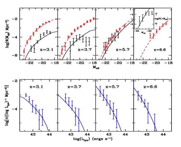
Figure 1: Top panels show the predicted UV LF of LBGs (dashed lines) at $z=3,4,6$ and $7$ and that of LAEs (thick lines) at $z=3.1,3.8,5.7$ and $6.6$ along with the observed data . The observed data points of LBGs taken from Bouwens et al. (2007, 2008) and Reddy et al. (2008) are shown as red filled squares. The black filled triangles are the observed UV LF data points from Ouchi et al. (2010, 2008). The insert in the top right panel shows the cumulative UV LF of LAEs (solid black lines) at $z=6.5$ as predicted by our models along with the data given by Kashikawa et al. (2011) (black filled triangles). Bottom panels show our model predictions of Lyman $\alpha$ LF of LAEs at $z=3.1,3.7,5.7$ and $6.6$. Here, the observed data points and error bars are from Ouchi et al. (2010, 2008)

The Lyman-$\alpha$ luminosity produced in any star forming region (when we use the case-B recombination) is related to its instantaneous star formation rate and is given by,

$$L_{Ly\alpha}=0.67h\nu_{\alpha}(1-f_{esc}){N}_{\gamma}{\dot{M}}_{SF}.$$ (3)

Here, $h\nu_{\alpha}=10.2$ eV is the energy of a Lyman-$\alpha$ photon and we fix $f_{esc}=0.1$, the escape fraction of UV ionizing photons. Further, ${N}_{\gamma}$ is the production rate of ionizing photon per unit solar mass of star formation which is a function of IMF and the metallicity. We use $N_{\gamma}=10450$ for the Salpeter IMF and metallicity of $Z=0.0004$ (See SSS07).

The observed Lyman-$\alpha$ luminosity is given by,

$$L_{Ly\alpha}^{obs}=f_{esc}^{Ly\alpha}L_{Ly\alpha}.$$ (4)

Here, $f_{esc}^{Ly\alpha}$ is the escape fraction of the Lyman-$\alpha$ photons which is decided by the dust optical depth, velocity field of the ISM in the galaxies and the Lyman-$\alpha$ optical depth due to ambient intergalactic medium around the galaxies.

Observations suggest that only a small fraction of LBGs ($G_{f}$) show detectable Lyman-$\alpha$ emission (See for example Kornei et al., 2010b). In our models we assume that the UV LF of LAEs at any $z$ is a fraction $G_{f}$ of the UV LF of LBGs at that redshift (i.e. $\Phi^{UV}_{LAE}=G_{f}\Phi^{UV}_{LBG}$). We estimate $G_{f}$ by comparing the model predictions of UV LF of LAEs with the observed data.

As a fiducial model we have chosen $\kappa=1.0$ at all redshifts and for $M_{agn}$, $0.8\times 10^{12}M_{\odot}$, $1.5\times 10^{12}M_{\odot}$ at redshifts $3$ and $4$. For higher redshifts we do not require any AGN feedback. As in SSS07 and J13, we find that with these parameters the observed luminosity functions is well reproduced for $f_{\ast}/\eta$ of 0.042, 0.038, 0.037 and 0.044 respectively for $z=3,4,6$ and $7$. We note that the values of $f_{\ast}/\eta$ is nearly constant over the redshift range considered. These values are tabulated in Table 1. If we use the average value of $\eta$ at $z=3-7$ estimated from Gonzalez et al. (2012); Reddy et al. (2012), we get $f_{\ast}=0.13-0.05$ in the same redshift range. This indicates an increase in the baryon fraction that is being converted into stars with time. In the top panel of Fig. 1 we show our model predictions of best fit UV LF of LBGs in dashed lines. The corresponding observational data is shown as solid squares.

The best fit values of $G_{f}$ that fits the UV LF of LAEs are also tabulated in Table 1. Our model predictions of UV LF of LAEs are shown in the top panels (in solid black lines) of Fig. 1 along with the observational data. At $z=6.6$, we compare our model predictions of cumulative UV LF of LAEs with the observed cumulative UV LF of LBGs given by Kashikawa et al. (2011) and fix $G_{f}$ to be 0.5 (See insert in the top right panel of Fig. 1). From the table it is clear that, $G_{f}$, the fraction of LBGs visible as LAEs increases from $\sim$ $0.05$ to $0.5$ from redshift $3-7$. Such a trend has been noted in the previous works of Stark et al. (2010); Pentericci et al. (2011); Curtis-Lake et al. (2012); Forero-Romero et al. (2012). These authors treat the fraction of LBGs visible as LAEs as a function of the UV magnitude of LBGs. However, the average fraction of fraction of LBGs visible as LAEs, obtained from their studies are consistent with our results.

Given $G_{f}$ one can obtain the Lyman-$\alpha$ LF of LAEs by varying $f_{*}f_{\rm esc}^{Ly\alpha}$ as a free parameter. In this way, the observed $Ly\alpha$ LFs of LAEs are well reproduced for $f_{\ast}f_{\rm esc}^{Ly\alpha}$ = $0.066,0.040,0.031$ and $0.029$ respectively at $z=3.1,3.8,5.7$ and $6.6$. These best fit $f_{*}f_{\rm esc}^{Ly\alpha}$ are tabulated in Table 1. We also show in the lower panels of Fig.1, our models predictions of the best fit Ly$\alpha$ LFs of LAEs along with observed data at different $z$. Using the $f_{\ast}$ determined earlier we have obtained $f_{\rm esc}^{Ly\alpha}=0.5-0.6$ in the redshift range $z=3.1-6.6$. Thus our models predicts no strong evolution in $f_{\rm esc}^{Ly\alpha}$ from $z=3.1$ to $6.6$ which is consistent with the earlier studies of Hayes et al. (2010); Blanc et al. (2011); Ono et al. (2010), who also found no clear evolution of $f_{\rm esc}^{Ly\alpha}$ in the above redshift range.

3 Two point correlation functions of LAEs

In this section we compute the angular correlation functions of high-$z$ LAEs on all angular scales. To do this, one requires the full knowledge of the halo occupation distribution (HOD). The HOD describes the probability distribution for galaxies brighter than a given luminosity threshold to reside in a dark matter halo of mass $M$ (Bullock et al., 2002; Berlind & Weinberg, 2002). Given the HOD, one can compute the average number of galaxies brighter than the luminosity threshold hosted by a dark matter halo of mass $M$. Further this information can be used with the halo model to calculate the galaxy correlation functions.

We modify the physically motivated HOD models of LBGs J13 to compute the same for LAEs that are brighter than a threshold Luminosity $L^{Ly\alpha}_{th}$. The mean number of galaxies inside a dark matter halo can be written as $N_{g}(M)=f_{cen}(M)+N_{s}(M)$ where $f_{cen}(M)$ and $N_{s}(M)$ are respectively the mean number of central and satellite galaxies. We also assume the central galaxy to be situated at the center of the halo and satellite galaxies following NFW density distribution of dark matter matter halos (Kravtsov et al., 2004).

3.1 The central galaxy occupation

In our model the luminosity $L$ of a galaxy initially increases and then decreases with its age. Therefore, a galaxy of mass $M$ collapsed at two different redshifts can shine with the same luminosity $L$ at a given observational redshift. Depending on the redshift of formation these galaxies will be either in their increasing phase or decreasing phase of luminosity. In between these two epochs (i.e. two redshifts) the galaxy will shine with luminosity greater than $L$. For such a model, the mean occupation number of central galaxies with a Lyman-$\alpha$ luminosity above a threshold luminosity (or magnitude) $L^{Ly\alpha}_{th}$ inside a halo of mass $M$ at any redshift $z$ as in Eq. (15) of J13 is

$$f_{cen}(L^{Ly\alpha}_{th},M,z)=G_{f}\frac{\int\limits_{z_{1}}^{z_{2}}dz_{c}\dfrac{dn(M,z_{c})}{dz_{c}}}{n(M,z)}.$$ (5)

Here $z_{1}(M,L^{Ly\alpha}_{th},z)$ and $z_{2}(M,L^{Ly\alpha}_{th},z)$ are the two redshifts at which a galaxy of mass $M$ is to be formed, so that it shines with an observed luminosity $L^{Ly\alpha}_{th}$ at $z$. Note a galaxy of mass $M$ that has collapsed between these two redshifts $z_{1}$ and $z_{2}$ will shine with a luminosity greater than $L^{Ly\alpha}_{th}$. We show in Fig 2 the halo mass $M$ that can host a galaxy of apparent magnitude, $m^{Ly\alpha}_{AB}=25.3$ (of the Lyman-$\alpha$ line) at $z=3.1$. Here, $m^{Ly\alpha}_{AB}$ is the narrow band apparent magnitude and can be computed from $L^{Ly\alpha}_{th}$ for a fixed set of cosmological parameters. The figure clearly shows that halos of any mass (above a minimum mass $M_{min}$) formed at two different redshifts can shine with the same magnitude at $z=3.1$. For example, when $M=10^{12}M_{\odot}$ (shown by dotted red horizontal line ) these two redshifts are approximately 3.13 and 5.9 For more details on the evaluation of $z_{1}$ and $z_{2}$ see Section (3) and Fig. (3) of J13.

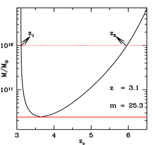
Figure 2: Masses of the dark matter halos that shine with an apparent magnitude $m^{Ly\alpha}_{AB}=25.3$ at $z=3.1$ as a function of their formation (collapse) redshift. Halos of a particular mass formed at two different redshifts can shine with the same brightness at $z=3.1$ which we refer as $z_{1}$ and $z_{2}$. For example, when $M=10^{12}M_{\odot}$ (shown by dotted red horizontal line) these two redshifts are approximately 3.13 and 5.94. The figure also shows in red horizontal solid line the minimum mass of the galaxy that can produce a magnitude 25.3 at $z=3.1$ which is roughly $2.4\times 10^{10}M_{\odot}$.

We also note that when $M<M_{min}(L^{Ly\alpha}_{th})$ the central galaxy occupation drops to zero, as galaxies below this mass scale can never posses a luminosity greater than $L^{Ly\alpha}_{th}$. For $m^{Ly\alpha}_{AB}=25.3$ and $z=3.1$ we have shown this threshold mass in Fig. 2. We have tabulated $M_{min}(L^{Ly\alpha}_{th})$ in Table 1 at each redshift. From this Table it can be seen that the $M_{min}$ is of the order of few times $10^{10}M_{\odot}$ at all redshifts and for all threshold magnitudes. These threshold masses of galaxies that can host an LAEs satisfying the threshold luminosities are roughly one order in magnitude smaller than lowest mass of LBGs with comparable threshold luminosities in UV light (see Table 3 of J13).

In Fig. 3 we have plotted as thin lines, the average occupation number of central galaxies ($f_{cen}(M)$) as function of the mass of the parent halo, calculated using the above prescription at different redshifts. For computing the $f_{cen}$ we have used $G_{f}$ and $f_{*}f_{\rm esc}^{Ly\alpha}$ which best fits the UV LF and and Ly$\alpha$ LF of LAEs.

3.1.1 The satellite galaxy occupation

Following J13 we have used the progenitor mass function and our star formation prescription to obtain an estimate of the number of subhalos and thereby the number of satellite LAEs hosted by a halo of mass $M$. The conditional mass function (Mo & White, 1996) gives the comoving number density of subhalos of mass $M_{s}$ which formed at $z_{s}$ inside a region containing a mass $M$ (or comoving volume $V$) that have a density contrast $\delta$ at $z_{p}<z_{s}$. To begin with, J13 consider regions of mass $M$ which have already formed virialized halos by the observational redshift $z$. In this limit the conditional mass function gives the mass function of subhalos in the mass range $M_{s}$ and $M_{s}+dM_{s}$ at $z_{s}$ inside a halo of mass $M$ that collapsed at $z<z_{p}<z_{s}$. The time derivative of this conditional mass function is taken as the formation rate of subhalos of mass $M_{s}$ inside a big halo of mass $M$. This is because as in J13 we assume that even though dark matter halos are created and destroyed inside the over dense volume of mass $M$, the satellite galaxies formed in these subhalos have survived and can be observed. The star formation models for the satellite galaxies are taken to be the same as that of central galaxies (given by Eq. (2)). This is similar to the assumption used by previous authors (Lee et al., 2009; Berrier et al., 2006; Conroy et al., 2006) where feedback due to halo merging processes are ignored.

We further assume in our models that no subhalo should be formed very close to the formation epoch of parent halo. More precisely if $t(z_{p})$ is the age of the universe when a parent halo collapsed then all the subhalos formed inside that parent halo within a time interval $\Delta t_{0}$ prior to $t(z_{p})$ do not host a satellite galaxy; rather they will be part of the parent halo itself. Thus in our models $t(z_{p})-t(z_{s})\geq\Delta t_{0}$ where $t(z_{s})$ is the age of the universe when the subhalo is formed inside the parent halo. The time scale $\Delta t_{0}$ is of the order of dynamical time scale of the parent halo. J13 showed that this formalism predicts the occupation of satellite galaxies $N_{s}(M,L_{th},z)$ that can successfully explain the small scale angular clustering of LBGs with $\Delta t_{0}$ of the order of dynamical time scale $t_{dyn}$ of the parent halo. For predicting the occupation of Lyman-$\alpha$ emitting satellites, we again assumed $\Delta t_{0}\geq t_{dyn}$. Interested readers may refer to Section (4.1.2) of J13 for more details.

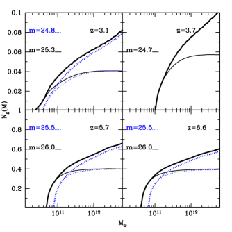
Figure 3: The halo occupation distribution, $\langle N_{g}(M)=f_{cen}(M)+N_{s}(M)\rangle$, as a function of the mass of the hosting halo, as predicted by our models at various redshifts and threshold magnitudes. In each panel the thin curves corresponds to $f_{cen}(M)$ where as the thick curves give the total occupation $N_{g}(M)=f_{cen}(M)+N_{s}(M)$. The solid and dotted lines correspond to two different threshold magnitudes. The curves are obtained using a fiducial set of model parameters (given in Section 2) that reproduce the observed luminosity function. In addition to that, to obtain the satellite occupation ($N_{s}(M)$), we have adopted $\Delta t_{0}=2.0t_{dyn}$ (see text for details).

3.1.2 The total halo occupation

We have plotted in Fig. 3 the total occupation number of galaxies, $N_{g}(M)=f_{cen}(M)+N_{s}(M)$ as a function of the mass of the parent halos at various redshifts and for different threshold magnitudes (i.e. $m^{Ly\alpha}_{AB})$. For each $z$ we have used the best fitted parameters given in Table 1. These curves are shown in thick lines and thin lines correspond to occupation number of central galaxies. To obtain $N_{s}(M)$, apart from the fiducial model parameters that fit the observed luminosity function, we have adopted $\Delta t_{0}=2t_{dyn}$. These values of $\Delta t_{0}$ are chosen as they are later used in Section 4 for explaining the small angular scale clustering. We find that for each limiting magnitude the mean numbers of central and satellite galaxies are monotonically increasing with the mass of the hosting halo mass.

It is of interest to calculate the average value of $N_{g}(M)=f_{cen}(M)+N_{s}(M)$, which is the average number of LAEs occupied in dark matter halos above the threshold mass $M_{min}$. As in J13 we define this quantity as

$$\langle N_{g}\rangle(L^{Ly\alpha}_{th},z)=\frac{\int_{M_{min}}^{\infty}dM\left(f_{cen}(M,z)+N_{s}(M,z)\right)n(M,z)}{\int_{M_{min}}^{\infty}dMn(M,z)}.$$ (6)

We give the value of $\langle N_{g}\rangle$ in Table 1 for different magnitude thresholds and redshifts. From this table it is clear that at $z=3.1$ there is about 1-2 % of LAEs in dark matter halos above the threshold mass $M_{min}$. This number is much smaller than that of LBGs (see Table 3 of J13) which was roughly 40%. However as we go to higher redshift, the average $N_{g}$ of LAEs increases. For $z\geq 5.7$ this is roughly 20 % which is roughly 50 % of the mean occupation of LBGs at higher redshifts. The mean $N_{g}$ described above can be invoked as the duty cycle of LAEs (see Lee et al. (2009), J13) hence this directly implies that LAEs have a smaller duty cycle compared to LBGs.

Similarly in Table 1, we also give the average mass $M_{av}$ of a halo hosting the LAEs, for each redshift and luminosity threshold. This average mass is defined as,

$$M_{av}=\frac{\int_{0}^{\infty}dMM\left(f_{cen}(M,z)+N_{s}(M,z)\right)n(M,z)}{\int_{0}^{\infty}dMf_{cen}(M,z)n(M,z)}.$$ (7)

One can find from Table 1 that the average mass of LAEs of the order of $10^{10}-10^{11}M_{\odot}$ at all redshifts and threshold magnitudes we are considering. For example, at $z=3.1$ and for $m_{AB}^{Ly\alpha}=25.3$ we find that $M_{av}=7\times 10^{10}M_{\odot}$ and at $z=5.7$ for $m_{AB}^{Ly\alpha}=25.5$ $M_{av}=1.4\times 10^{11}M_{\odot}$. Further, at a given redshift, $M_{av}$ of LAEs increases with higher threshold luminosity. We also note that, the average masses halos, hosting LBGs brighter than similar continuum magnitude, are higher by an order of magnitude (given in Table 3 of J13). For example at $z=4$, the average mass of LBGs brighter than $m_{AB}^{UV}=25.5$ is $5.6\times 10^{11}M_{\odot}$, which is roughly ten times bigger than that of LAEs brighter than $m_{AB}^{Ly\alpha}=25.3$. This is in agreement with the suggestions that LAEs are residing in smaller mass halos compared to LBGs (Ouchi et al., 2010).

$z$	$f_{\ast}/\eta$	$G_{f}$	$f_{\ast}f^{Ly\alpha}_{esc}$	$m_{AB}^{Ly\alpha}$	$log(L_{Ly\alpha})$	$M_{min}/M_{\odot}$	$M_{av}/M_{\odot}$	$\langle N_{g}\rangle$	$n_{g}$	$b_{g}$	$b_{g}(O)$
$\sim$ 3.1	0.042	0.041	0.066	25.3	42.1	$2.4\times 10^{10}$	$7.1\times 10^{10}$	0.011	1.8	2.1	1.5 $\pm$ 0.7
				24.8	42.3	$3.8\times 10^{10}$	$9.6\times 10^{10}$	0.014	1.1	2.2	1.5 $\pm$ 0.3
$\sim$ 3.7	0.038	0.059	0.040	24.7	42.6	$10^{11}$	$2.2\times 10^{11}$	0.024	0.4	3.5	2.8 $\pm$ 0.5
$\sim$ 5.7	0.037	0.421	0.031	26.0	42.4	$5.0\times 10^{10}$	$9.1\times 10^{10}$	0.190	1.8	5.1	5.5 $\pm$ 0.4
				25.5	42.6	$7.9\times 10^{10}$	$1.4\times 10^{11}$	0.180	0.8	5.6	6.1 $\pm$ 0.7
$\sim$ 6.6	0.044	0.50	0.029	26.0	42.4	$4.3\times 10^{10}$	$7.5\times 10^{10}$	0.230	1.1	6.1	3.6 $\pm$ 0.7
				25.5	42.6	$6.8\times 10^{10}$	$1.2\times 10^{11}$	0.213	0.5	6.7	6.0 $\pm$ 2.2

Table 1: Best fitted and derived parameters of our models. (1) Redshift; (2) $f_{\ast}/\eta$, the parameter related to the light to mass ratio of galaxies; (3) $G_{f}$, the fraction of LBGs that shows detectable Ly$\alpha$ emission; (4) $f_{\ast}f^{Ly\alpha}_{esc}$, the parameter related to the net Ly$\alpha$ emission from LAEs; (5) the limiting magnitude of LAE samples; (6) approximated limiting Ly$\alpha$ luminosity corresponding to $m_{AB}^{Ly\alpha}$; (7) minimum mass of dark matter matter halos that can host LAEs brighter than $m_{AB}^{Ly\alpha}$; (8) average mass of dark matter matter halos that can host LAEs brighter than $m_{AB}^{Ly\alpha}$; (9) average occupation of LAEs in dark matter halos; (10) number density of LAEs in units of $10^{-3}(h/Mpc)^{3}$; (11) large scale galaxy bias of LAEs of the given threshold magnitude; (12) best estimate of bias by Ouchi et al. (2010).

3.2 The correlation functions.

In the framework of halo model, the total correlation function can be written as (Cooray & Sheth, 2002)

$$\xi_{g}(R)=\xi^{1h}_{g}(R,z)+\xi^{2h}_{g}(R,z)$$ (8)

where each term on RHS has contributions from central as well as satellite galaxies. On scales much bigger than the virial radius of a typical halo, the clustering amplitude is dominated by correlations between galaxies inside separate halos (called the 2-halo term or $\xi^{2h}_{g}$). On the other hand, on scales smaller than the typical virial radius of a dark matter halo, the major contribution to galaxy clustering is from galaxies residing in the same halo (called the 1-halo term or $\xi^{1h}_{g}$).

The 2 halo term, $\xi^{2h}_{g}(r,z,L^{Ly\alpha}_{th})$, of galaxies with luminosity greater than $L^{Ly\alpha}_{th}$ at $z$, can now be calculated using (Peebles, 1980),

$$\xi^{2h}_{g}(R,z,L^{Ly\alpha}_{th})=\int_{0}^{\infty}\frac{dk}{2\pi^{2}}k^{2}\frac{\sin(kR)}{kR}P^{2h}_{g}(k,z,L^{Ly\alpha}_{th}).$$ (9)

Here $P_{g}^{2h}(k,L^{Ly\alpha}_{th},z)$ is the luminosity dependent galaxy power spectrum, which is computed as

$$P_{g}^{2h}(k,L^{Ly\alpha}_{th},z)=b^{2}_{g}(k,L^{Ly\alpha}_{th},z)P_{lin}(k,z).$$ (10)

In the above equation, $P_{lin}(k,z)$, is the linear power spectrum of CDM density fluctuations. The luminosity dependent galaxy bias obtained by adding the contributions of both the central and satellite galaxies is,

$$b_{g}(k,z,L^{Ly\alpha}_{th})=\frac{1}{n^{T}_{g}(L^{Ly\alpha}_{th},z)}\int dMn(M,z)b(M,z)$$

$$~{}~{}~{}~{}~{}~{}~{}\Big{[}f_{cen}(L^{Ly\alpha}_{th},M,z)+\langle N_{s}|L^{Ly\alpha}_{th},M,z)\rangle\Big{]}$$

$$u(k,M,z).$$ (11)

As before, $n(M,z)$ is the ST halo mass function, and

$$n^{T}_{g}(L^{Ly\alpha}_{th},z)=\int dMn(M,z)(f_{cen}(M,z)+\langle N_{s}|L^{Ly\alpha}_{th},M,z\rangle)$$ (12)

is the total number density of galaxies, including both central and satellite galaxies. Further, $b(M,z)$ is the mass dependent halo bias factor provided by the fitting function of Sheth and Tormen (Sheth & Tormen, 1999; Cooray & Sheth, 2002, also see Eq. (7) of J13). In Eq. (11) $u(k,M)$ is the Fourier transform of dark matter density profile normalized by its mass, i.e $u(k,M,z)=\bar{\rho}(k,M,z)/M$. For the present calculations we use the Navarro Frenk White (NFW) form for the dark matter density distribution (Navarro et al., 1997). On scales much larger than the virial radius of typical halos $u(k,M,z)=1$ and hence the luminosity dependent galaxy bias given by Eq. 11 becomes a constant.

We give in Table 1 this constant galaxy bias computed using our models. We note that the large scale galaxy bias predicted by our models compares well with observationally derived galaxy bias from Ouchi et al. (2010) (given in the last column of Table 1) at each redshift and for nearly all threshold luminosities. We also find that the galaxy bias for a given $z$ increases with increasing luminosity and is systematically higher for high redshift galaxies. Further, the large scale bias, computed here for LAEs brighter than a given Lyman $\alpha$ threshold luminosity, is smaller than that LBGs brighter than the same continuum luminosity (see Table 2 of J13). This result has been observed previously by Ouchi et al. (2010). This is because, as we have seen in the last section, LAEs of given Lyman $\alpha$ luminosity are residing in dark matter halos of smaller mass compared to LBGs of the same continuum UV luminosity. This directly results in smaller clustering strength of LAEs compared to LBGs. We elaborate on this interesting fact in the next section.

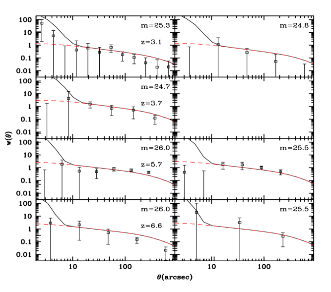
Figure 4: The angular correlation function of LAEs, taking into account the one halo and the two halo terms, at redshifts 3.1, 3.8, 5.7 and 6.6 for various limiting magnitudes. Each row corresponds to a particular redshift, which is labelled in the first panel of that row. In each panel clustering predictions for galaxies with a given threshold magnitude is shown. Our fiducial model predictions of galaxy angular correlation functions with $\Delta t_{0}=2t_{dyn}$ is shown in solid black lines. The dashed red curves are our model predictions assuming a sub-Poisson distribution for galaxies inside dark matter halos (see text for details). The data points and error bars shown by black open rectangles are from Ouchi et al. (2010).

3.3 The total correlation functions

The 1-halo term $\xi^{1h}_{g}(R)$ uses the standard assumption that radial distribution of satellite galaxies inside a parent halo follows the dark matter density distribution (NFW profile) (Cooray & Sheth, 2002). In this case the 1-halo term is given by (Tinker et al., 2005; Cooray & Ouchi, 2006)

$$\xi^{1h}(L^{Ly\alpha}_{th},R,z)=\frac{1}{(n_{g}^{T})^{2}}\int dM~{}n(M,z)\Big{[}2f_{cen}(L^{Ly\alpha}_{th},M,z)$$

$$~{}~{}\langle N_{s}|L^{Ly\alpha}_{th},M,z\rangle\frac{\rho_{NFW}(R|M)}{M}+$$

$$~{}~{}\langle N_{s}(N_{s}-1)|L^{Ly\alpha}_{th},M,z\rangle\frac{\lambda_{NFW}(R|M)}{M^{2}}\Big{]}.$$ (13)

Here, as before, $n^{T}_{g}(L^{Ly\alpha}_{th},z)$ is the total number density of galaxies which includes both the central and satellite galaxies. Further $\rho_{NFW}$ is the NFW profile of dark matter density (Navarro et al., 1997) inside a collapsed halo and $\lambda_{NFW}(r|M)$ is the convolution of this density profile with itself (Sheth et al., 2001). For the halo concentration parameter we use the fitting functions given by Prada et al. (2012) (Eq. (14-23) of their paper). Also to begin with, following the N-body simulations and semi-analytical models (eg.  Kravtsov et al., 2004; Zheng et al., 2005), we assume that the number of satellites inside a parent halo forms a Poisson distribution. Thus we have $\langle N_{s}(N_{s}-1)\rangle=N^{2}_{s}$, when $N_{g}$ is large.

Finally we compute luminosity dependent angular correlation function $w(\theta,z)$ from the spatial correlation function using Limber equation (Peebles, 1980, J13)

$$w(\theta,z)=\int_{0}^{\infty}dz^{\prime}~{}N(z^{\prime})\int_{0}^{\infty}dz^{\prime\prime}~{}N(z^{\prime\prime})\xi_{g}\left(z,r(\theta;z^{\prime},z^{\prime\prime})\right)$$ (14)

where $r(\theta;z^{\prime},z^{\prime\prime})$ is the comoving separation between two points at $z^{\prime}$ and $z^{\prime\prime}$ subtending an angle $\theta$ with respect to an observer today. Here we have also incorporated the normalized redshift selection function, $N(z)$, of the observed population of galaxies given in Ouchi et al. (2010, 2008). In Eq. (14) we neglect the redshift evolution of clustering of the galaxies detected around $z$. Hence the spatial two-point correlation function $\xi_{g}(r,z)$ is always evaluated at the observed redshift.

4 Comparisons with observations

The total angular correlation functions computed using our prescription for four redshifts and two threshold magnitudes are overplotted on the observed data in Fig. 4. The cosmological parameters, $M_{agn}$ and $\kappa$ are kept to their fiducial value. All these models assumes $\Delta t_{0}=2~{}t_{dyn}$. All other model parameters are obtained by fitting the LFs and are given in Table 1. It is important to note that, we compare our model predictions of LF and clustering of LAEs with that of LAEs in the Subaru/XMM-Newton Deep Survey (SXDS) Field (Ouchi et al., 2008, 2010; Kashikawa et al., 2011). In particular, the clustering data of LAEs provided by Ouchi et al. (2010) is for galaxies selected purely by their narrow band magnitude limits irrespective of whether those galaxies are detected in UV or not.

Firstly, we note that angular correlation functions predicted by our model (for $\theta\geq 10^{\prime\prime}$) is in very good agreement with the observed data at all redshifts and for all threshold luminosities. The amplitudes of these angular correlation functions are higher than that of LBGs (see Fig. 9 of J13) mainly because LAEs have a much narrower redshift distribution function $N(z)$.

We note that our models systematically overpredicts clustering at very small angular scales ($\theta\leq 10^{\prime\prime}$) at all redshifts and for all magnitudes. That is the contribution of one halo term predicted by our models to the $w(\theta)$ for small values of $\theta$ is not distinctly evident from the observed $w(\theta)$. We now investigate whether this discrepancy could be due to our earlier assumption that galaxies are Poisson distributed in dark matter halos. N-body simulations (eg. Kravtsov et al., 2004) showed that the HOD follows a Poisson distribution when the total number of galaxies inside a halo exceeds unity. Number of earlier works (Scoccimarro et al., 2001; Wechsler et al., 2001; Bullock et al., 2002) have pointed out that, galaxies follow sub-Poisson distribution when $N_{g}(M)\leq 1$. Note from Fig 3, the average halo occupation ($\langle N_{g}\rangle$) of LAEs ($3.1\leq z\leq 6.6$) in dark matter halos are typically smaller than unity. Therefore we choose the model of Bullock et al. (2002) (see also Hamana et al., 2004) for the average number of galaxy pairs inside a dark matter halo of mass $M$,

$$\langle N_{g}(N_{g}-1)(M)\rangle=\begin{cases}N^{2}_{g}(M)&\text{$N_{g}\geq 1$}\\ N^{2}_{g}(M)~{}\dfrac{ln(4N_{g}(M))}{ln(4)}&\text{$0.25<N_{g}<1$}\\ 0&\text{$N_{g}\leq 0.25$}\end{cases}$$ (15)

In this case the 1-halo term is computed as in Hamana et al. (2004), where

$$\xi^{1h}(L^{Ly\alpha}_{th},R,z)=\frac{1}{(n_{g}^{T})^{2}}\int dM~{}n(M,z)$$

$$\langle N_{g}(N_{g}-1)|L^{Ly\alpha}_{th},M,z\rangle\frac{\lambda_{NFW}(R|M)}{M^{2}}.$$ (16)

In Fig. 4 we show our model predictions (in red dashed lines) when one uses the above sub-Poisson distribution for galaxy occupation. One can see from the figure that our model predictions of angular correlation functions are consistent with the observed data even at very small angular scales ($\theta\leq 10^{\prime\prime}$) for all redshifts and threshold magnitudes.

As discussed earlier, galaxies selected by their threshold AB magnitude in Lyman $\alpha$ luminosity, are less strongly clustered than the galaxies selected by same UV threshold AB magnitude (See Fig. 9 and Table 2 of J13 also). This can be understood in the following way. In Fig. 5 we have plotted the difference in the observed Lyman $\alpha$ and UV magnitudes of LAEs at $z=3.1$ against their Lyman $\alpha$ magnitudes. The data points are from from Ouchi et al. (2008). The figure clearly shows that the observed Lyman $\alpha$ apparent magnitude of LAEs residing in a halo of given mass are higher than their continuum magnitude roughly by a factor of $\Delta m_{AB}=m_{AB}^{UV}-m_{AB}^{Ly\alpha}\sim 2$. Or equivalently, the Lyman $\alpha$ line luminosity of LAEs are typically higher than their continuum UV luminosity by a factor $10^{0.8}$. This inturn implies that, LAEs of a given Lyman $\alpha$ luminosity, can be found in low mass dark matter halos compared to an LBG of the same UV threshold magnitude. As a result, the galaxy bias of LAEs of a given Lyman $\alpha$ threshold magnitude are smaller than LBGs of the same threshold magnitude in UV.

Figure 5: A comparison of the Lyman $\alpha$ AB magnitudes ($m_{AB}^{Ly\alpha}$) and UV AB magnitudes ($m_{AB}^{UV}$) of observed Lyman $\alpha$ emitters at $z=3.1$. The Y-axis shows the difference between UV and Lyman $\alpha$ magnitudes. The data points are from Ouchi et al. (2008).

The above discussions suggest that at $z=3.1$, the galaxy bias of LAEs with a line threshold magnitude, $m_{AB}^{Ly\alpha}$, must be comparable to the galaxy bias of LBGs with continuum threshold magnitude, $m_{AB}^{UV}$, where $m_{AB}^{UV}\sim m_{AB}^{Ly\alpha}+2$. In order to demonstrate this more elaborately, we computed the galaxy bias of LBGs (using the prescription of J13) at $z=3.1$ for threshold magnitude $m_{AB}^{UV}=26.8$ and compared it with that of LAEs of threshold magnitude $m_{AB}^{Ly\alpha}=24.8$ (here $\Delta m_{AB}=2$). Interestingly we found that at $z=3.1$ galaxy bias of LBG samples (using the best fitted parameters of LBG LF) with $m_{AB}^{UV}=26.8$ is $b_{g}=2.35$ which compares very well with galaxy bias of $b_{g}=2.2$ that we obtain for LAEs with $m_{AB}^{Ly\alpha}=24.8$. Further, the average mass of these LBGs is $9.9\times 10^{10}M_{\odot}$, which is very similar to the average mass, $9.6\times 10^{10}M_{\odot}$, of LAEs with $m_{AB}^{Ly\alpha}=24.8$. We performed similar exercise at other redshifts and found comparable galaxy bias and average mass for LAEs and LBGs when appropriate limiting magnitude are chosen. This implies that the connection between dark matter halo and UV luminosity found by J13 for the LBGs is valid for the LAEs as well.

5 Discussion and conclusions

We have presented here a physically motivated semi-analytical model of galaxies to understand the clustering of high redshift Lyman-$\alpha$ emitters. In our models we assign luminosities (UV and Ly$\alpha$) to galaxies residing in dark matter halos by a physical model of star formation. The free parameters of this star formation model are then constrained by the observed high redshift luminosity functions. Further using the semi analytical approach of J13, we combined these constrained models of star formation with the halo model and predicted the angular correlation functions, $w(\theta)$ of LAEs. Our model predictions of $w(\theta)$ of LAEs with different threshold magnitudes compares remarkably well with the observed data of Ouchi et al. (2010) for $\theta\geq 10^{\prime\prime}$ in the redshift range $z\sim 3-7$.

Our models assumed that only a fraction $G_{f}$ of halos hosting LBGs produce a detectable amound of Lyman-$\alpha$ luminosity. The low amplitudes of LFs LAEs compared to that of LBGs at various redshifts suggest that $G_{f}$ is typically smaller than unity. We found that $G_{f}$ ranges from $4\%-50\%$ in the redshift range $3.1-6.6$. Such small values of $G_{f}$ directly result in a low halo occupation for LAEs compared to LBGs. Our models for LBG halo occupation (see J13) suggested that about 40% dark matter halos above a minimum mass $M_{min}$ host LBGs above a threshold luminosity. On the other hand, the average number LAEs occupying dark matter halos, $\langle N_{g}\rangle$, are much smaller, ranging from $1\%-23\%$ in the above redshift range. As low halo occupation is related to duty cycle (see J13), we can conclude that Lyman-$\alpha$ emission has much smaller duty cycle compared to the UV emitting phase of the high redshift galaxies.

We find that, for observationally determined $\eta$ from Bouwens et al. (2012); Reddy et al. (2012) studies at various redshifts, the escape fraction of Lyman-$\alpha$ from LAEs varies from $\sim 0.5$ to $\sim 0.6$ for the redshift range $3.1\leq z\leq 6.6$. Thus in our studies $f^{Ly\alpha}_{esc}$ is not strongly evolving in the above redshift range and such a trend is consistent with previous studies. The lack of sharp decrease in $f^{Ly\alpha}_{esc}$ in this redshift range is consistent with the epoch of reionization $z_{re}\geq 6.6$. Such large values of $f^{Ly\alpha}_{esc}$ are consistent with previous studies and can be explained by clumped models of interstellar medium (Neufeld, 1991; Dayal et al., 2010; Forero-Romero et al., 2010).

We found that the average masses, $M_{av}$ of halos hosting LAEs brighter than any threshold Lyman-$\alpha$ luminosity are smaller than that of LBGs brighter than similar continuum threshold luminosity. For Lyman $\alpha$ apparent magnitudes 25-26, $M_{av}$ ranges typically from $7.0\times 10^{10}M_{\odot}-1.2\times 10^{11}M_{\odot}$ and are smaller than typical LBGs of similar continuum magnitude by a factor 10. Because of their smaller halo masses, LAEs brighter than a given threshold line luminosity have smaller galaxy bias and are more weakly clustered than LBGs brighter than similar continuum luminosities. Our model predictions of galaxy bias compares very well with observationally derived galaxy bias of Ouchi et al. (2010). We also found that, the smaller masses and biases of LAEs brighter than a given line luminosity compared to LBGs brighter than similar continuum luminosity is the simple consequence of the fact that line luminosity of LAEs are typically higher than their continuum UV luminosity. In particular, Fig. 5 shows that the difference between the observed continuum magnitude, $m^{UV}_{AB}$, and line magnitude, $m^{Ly\alpha}_{AB}$, of LAEs at $z=3.1$ is $\Delta m_{AB}\sim 2$. We further showed that the galaxy bias of LBG sample with $m^{UV}_{AB}=26.8$ is almost same as the galaxy bias of LAEs with $m^{Ly\alpha}_{AB}=24.8$. In addition the average mass derived for these LBGs ($m^{UV}_{AB}=26.8$) is very much comparable to the average mass of LAEs with $m_{AB}^{Ly\alpha}=24.8$. This clearly suggests that LAEs belong to the same galaxy population of LBGs with narrow band technique having more efficiency in picking up galaxies with low UV luminosity or low mass.

Finally we note that our simple model, that uses Poisson distribution for satellite galaxies in dark matter halos, predicts an excess in the small angular scale ($\theta\leq 10^{\prime\prime}$) clustering. The angular correlation functions on these scales are dominated by one halo term. We demonstrate that this discrepancy can be removed if one uses a sub-Poisson distribution for galaxies inside dark matter halos when the total galaxy occupation $N_{g}$ is smaller than unity. Since $G_{f}$ is always smaller than unity, our models predict a low occupation of LAEs in dark matter halos (See Fig 3) for all redshifts and for various threshold magnitudes. The total occupation, $N_{g}$ is bigger than unity only for very massive dark matter halos. The small angular scale clustering of LAEs can in principle be used constrain the statistics of galaxy occupation in dark matter halos when the mean occupation, $N_{g}$, is smaller than unity.

We have shown that the clustering of LAEs can be understood in the framework of halo model and physical models of galaxy formation. A clear understanding of these LAEs requires the complete knowledge of Lyman-$\alpha$ radiative transport in the interstellar medium. Nevertheless, our simple model suggests that, LAEs belong to the same galaxy population as LBGs and narrow band techniques are picking up galaxies with strong Lyman-$\alpha$ lines.

References

- Adelberger et al. (1998) Adelberger K. L., Steidel C. C., Giavalisco M., Dickinson M., Pettini M., Kellogg M., 1998, ApJ, 505, 18
- Beckwith et al. (2006) Beckwith S. V. W. et al., 2006, AJ, 132, 1729
- Benson et al. (2002) Benson A. J., Lacey C. G., Baugh C. M., Cole S., Frenk C. S., 2002, MNRAS, 333, 156
- Berlind & Weinberg (2002) Berlind A. A., Weinberg D. H., 2002, ApJ, 575, 587
- Berrier et al. (2006) Berrier J. C., Bullock J. S., Barton E. J., Guenther H. D., Zentner A. R., Wechsler R. H., 2006, ApJ, 652, 56
- Best et al. (2006) Best P. N., Kaiser C. R., Heckman T. M., Kauffmann G., 2006, MNRAS, 368, L67
- Bielby et al. (2011) Bielby R. M. et al., 2011, MNRAS, 414, 2
- Blanc et al. (2011) Blanc G. A. et al., 2011, ApJ, 736, 31
- Bouwens et al. (2007) Bouwens R. J., Illingworth G. D., Franx M., Ford H., 2007, ApJ, 670, 928
- Bouwens et al. (2008) Bouwens R. J., Illingworth G. D., Franx M., Ford H., 2008, ApJ, 686, 230
- Bouwens et al. (2012) Bouwens R. J. et al., 2012, ApJ, 754, 83
- Bower et al. (2006) Bower R. G., Benson A. J., Malbon R., Helly J. C., Frenk C. S., Baugh C. M., Cole S., Lacey C. G., 2006, MNRAS, 370, 645
- Bromm & Loeb (2002) Bromm V., Loeb A., 2002, ApJ, 575, 111
- Bullock et al. (2002) Bullock J. S., Wechsler R. H., Somerville R. S., 2002, MNRAS, 329, 246
- Chiu & Ostriker (2000) Chiu W. A., Ostriker J. P., 2000, ApJ, 534, 507
- Choudhury & Srianand (2002) Choudhury T. R., Srianand R., 2002, MNRAS, 336, L27
- Conroy et al. (2006) Conroy C., Wechsler R. H., Kravtsov A. V., 2006, ApJ, 647, 201
- Cooray & Ouchi (2006) Cooray A., Ouchi M., 2006, MNRAS, 369, 1869
- Cooray & Sheth (2002) Cooray A., Sheth R., 2002, Phys. Rep., 372, 1
- Curtis-Lake et al. (2012) Curtis-Lake E. et al., 2012, MNRAS, 422, 1425
- Dawson et al. (2007) Dawson S., Rhoads J. E., Malhotra S., Stern D., Wang J., Dey A., Spinrad H., Jannuzi B. T., 2007, ApJ, 671, 1227
- Dayal & Ferrara (2012) Dayal P., Ferrara A., 2012, MNRAS, 421, 2568
- Dayal et al. (2008) Dayal P., Ferrara A., Gallerani S., 2008, MNRAS, 389, 1683
- Dayal et al. (2010) Dayal P., Ferrara A., Saro A., 2010, MNRAS, 402, 1449
- Dijkstra et al. (2004) Dijkstra M., Haiman Z., Rees M. J., Weinberg D. H., 2004, ApJ, 601, 666
- Dijkstra & Wyithe (2012) Dijkstra M., Wyithe J. S. B., 2012, MNRAS, 419, 3181
- Finkelstein et al. (2007) Finkelstein S. L., Rhoads J. E., Malhotra S., Pirzkal N., Wang J., 2007, ApJ, 660, 1023
- Forero-Romero et al. (2011) Forero-Romero J. E., Yepes G., Gottlöber S., Knollmann S. R., Cuesta A. J., Prada F., 2011, MNRAS, 415, 3666
- Forero-Romero et al. (2010) Forero-Romero J. E., Yepes G., Gottlöber S., Knollmann S. R., Khalatyan A., Cuesta A. J., Prada F., 2010, MNRAS, 403, L31
- Forero-Romero et al. (2012) Forero-Romero J. E., Yepes G., Gottlöber S., Prada F., 2012, MNRAS, 419, 952
- Garel et al. (2012) Garel T., Blaizot J., Guiderdoni B., Schaerer D., Verhamme A., Hayes M., 2012, MNRAS, 422, 310
- Gawiser et al. (2006) Gawiser E. et al., 2006, ApJ, 642, L13
- Giavalisco & Dickinson (2001) Giavalisco M., Dickinson M., 2001, ApJ, 550, 177
- Giavalisco et al. (2004) Giavalisco M. et al., 2004, ApJ, 600, L93
- Gonzalez et al. (2012) Gonzalez V., Bouwens R., llingworth G., Labbe I., Oesch P., Franx M., Magee D., 2012, ArXiv e-prints
- Grogin et al. (2011) Grogin N. A. et al., 2011, ApJS, 197, 35
- Gronwall et al. (2007) Gronwall C. et al., 2007, ApJ, 667, 79
- Hamana et al. (2004) Hamana T., Ouchi M., Shimasaku K., Kayo I., Suto Y., 2004, MNRAS, 347, 813
- Hayes et al. (2010) Hayes M. et al., 2010, Nature, 464, 562
- Hildebrandt et al. (2009) Hildebrandt H., Pielorz J., Erben T., van Waerbeke L., Simon P., Capak P., 2009, A&A, 498, 725
- Hu et al. (2010) Hu E. M., Cowie L. L., Barger A. J., Capak P., Kakazu Y., Trouille L., 2010, ApJ, 725, 394
- Hu et al. (1998) Hu E. M., Cowie L. L., McMahon R. G., 1998, ApJ, 502, L99
- Illingworth et al. (2013) Illingworth G. D. et al., 2013, ArXiv e-prints
- Jose et al. (2013) Jose C., Subramanian K., Srianand R., Samui S., 2013, MNRAS, 429, 2333
- Kashikawa et al. (2011) Kashikawa N. et al., 2011, ApJ, 734, 119
- Kashikawa et al. (2006) Kashikawa N. et al., 2006, ApJ, 637, 631
- Kobayashi et al. (2007) Kobayashi M. A. R., Totani T., Nagashima M., 2007, ApJ, 670, 919
- Kobayashi et al. (2010) Kobayashi M. A. R., Totani T., Nagashima M., 2010, ApJ, 708, 1119
- Kornei et al. (2010a) Kornei K. A., Shapley A. E., Erb D. K., Steidel C. C., Reddy N. A., Pettini M., Bogosavljević M., 2010a, ApJ, 711, 693
- Kornei et al. (2010b) Kornei K. A., Shapley A. E., Erb D. K., Steidel C. C., Reddy N. A., Pettini M., Bogosavljević M., 2010b, ApJ, 711, 693
- Kravtsov et al. (2004) Kravtsov A. V., Berlind A. A., Wechsler R. H., Klypin A. A., Gottlöber S., Allgood B., Primack J. R., 2004, ApJ, 609, 35
- Larson et al. (2011) Larson D. et al., 2011, ApJS, 192, 16
- Le Delliou et al. (2006) Le Delliou M., Lacey C. G., Baugh C. M., Morris S. L., 2006, MNRAS, 365, 712
- Lee et al. (2009) Lee K.-S., Giavalisco M., Conroy C., Wechsler R. H., Ferguson H. C., Somerville R. S., Dickinson M. E., Urry C. M., 2009, ApJ, 695, 368
- Lorenzoni et al. (2013) Lorenzoni S., Bunker A. J., Wilkins S. M., Caruana J., Stanway E. R., Jarvis M. J., 2013, MNRAS, 429, 150
- Madau et al. (1996) Madau P., Ferguson H. C., Dickinson M. E., Giavalisco M., Steidel C. C., Fruchter A., 1996, MNRAS, 283, 1388
- Mao et al. (2007) Mao J., Lapi A., Granato G. L., de Zotti G., Danese L., 2007, ApJ, 667, 655
- McLure et al. (2012) McLure R. J. et al., 2012, ArXiv e-prints
- Mo & White (1996) Mo H. J., White S. D. M., 1996, MNRAS, 282, 347
- Nagamine et al. (2010) Nagamine K., Ouchi M., Springel V., Hernquist L., 2010, PASJ, 62, 1455
- Navarro et al. (1997) Navarro J. F., Frenk C. S., White S. D. M., 1997, ApJ, 490, 493
- Neufeld (1991) Neufeld D. A., 1991, ApJ, 370, L85
- Oesch et al. (2013) Oesch P. A. et al., 2013, ArXiv e-prints
- Ono et al. (2010) Ono Y., Ouchi M., Shimasaku K., Dunlop J., Farrah D., McLure R., Okamura S., 2010, ApJ, 724, 1524
- Ouchi et al. (2005) Ouchi M. et al., 2005, ApJ, 635, L117
- Ouchi et al. (2008) Ouchi M. et al., 2008, ApJS, 176, 301
- Ouchi et al. (2003) Ouchi M. et al., 2003, ApJ, 582, 60
- Ouchi et al. (2010) Ouchi M. et al., 2010, ApJ, 723, 869
- Ouchi et al. (2004a) Ouchi M. et al., 2004a, ApJ, 611, 660
- Ouchi et al. (2004b) Ouchi M. et al., 2004b, ApJ, 611, 685
- Peebles (1980) Peebles P. J. E., 1980, The large-scale structure of the universe
- Pentericci et al. (2011) Pentericci L. et al., 2011, ApJ, 743, 132
- Pentericci et al. (2007) Pentericci L., Grazian A., Fontana A., Salimbeni S., Santini P., de Santis C., Gallozzi S., Giallongo E., 2007, A&A, 471, 433
- Prada et al. (2012) Prada F., Klypin A. A., Cuesta A. J., Betancort-Rijo J. E., Primack J., 2012, MNRAS, 3206
- Reddy et al. (2012) Reddy N. A., Pettini M., Steidel C. C., Shapley A. E., Erb D. K., Law D. R., 2012, ApJ, 754, 25
- Reddy & Steidel (2009) Reddy N. A., Steidel C. C., 2009, ApJ, 692, 778
- Reddy et al. (2008) Reddy N. A., Steidel C. C., Pettini M., Adelberger K. L., Shapley A. E., Erb D. K., Dickinson M., 2008, ApJS, 175, 48
- Rhoads et al. (2000) Rhoads J. E., Malhotra S., Dey A., Stern D., Spinrad H., Jannuzi B. T., 2000, ApJ, 545, L85
- Samui et al. (2007) Samui S., Srianand R., Subramanian K., 2007, MNRAS, 377, 285
- Samui et al. (2009) Samui S., Srianand R., Subramanian K., 2009, MNRAS, 398, 2061
- Savoy et al. (2011) Savoy J., Sawicki M., Thompson D., Sato T., 2011, ApJ, 737, 92
- Schenker et al. (2013) Schenker M. A. et al., 2013, ApJ, 768, 196
- Scoccimarro et al. (2001) Scoccimarro R., Sheth R. K., Hui L., Jain B., 2001, ApJ, 546, 20
- Sheth et al. (2001) Sheth R. K., Hui L., Diaferio A., Scoccimarro R., 2001, MNRAS, 325, 1288
- Sheth & Tormen (1999) Sheth R. K., Tormen G., 1999, MNRAS, 308, 119
- Shimasaku et al. (2006a) Shimasaku K. et al., 2006a, PASJ, 58, 313
- Shimasaku et al. (2006b) Shimasaku K. et al., 2006b, PASJ, 58, 313
- Shioya et al. (2009) Shioya Y. et al., 2009, ApJ, 696, 546
- Stark et al. (2010) Stark D. P., Ellis R. S., Chiu K., Ouchi M., Bunker A., 2010, MNRAS, 408, 1628
- Steidel et al. (1998) Steidel C. C., Adelberger K. L., Dickinson M., Giavalisco M., Pettini M., Kellogg M., 1998, ApJ, 492, 428
- Steidel et al. (1999) Steidel C. C., Adelberger K. L., Giavalisco M., Dickinson M., Pettini M., 1999, ApJ, 519, 1
- Steidel et al. (1996) Steidel C. C., Giavalisco M., Dickinson M., Adelberger K. L., 1996, AJ, 112, 352
- Tilvi et al. (2009) Tilvi V., Malhotra S., Rhoads J. E., Scannapieco E., Thacker R. J., Iliev I. T., Mellema G., 2009, ApJ, 704, 724
- Tinker et al. (2005) Tinker J. L., Weinberg D. H., Zheng Z., Zehavi I., 2005, ApJ, 631, 41
- Wang et al. (2009) Wang J.-X., Malhotra S., Rhoads J. E., Zhang H.-T., Finkelstein S. L., 2009, ApJ, 706, 762
- Wechsler et al. (2001) Wechsler R. H., Somerville R. S., Bullock J. S., Kolatt T. S., Primack J. R., Blumenthal G. R., Dekel A., 2001, ApJ, 554, 85
- Zheng et al. (2005) Zheng Z. et al., 2005, ApJ, 633, 791
- Zheng et al. (2010) Zheng Z., Cen R., Trac H., Miralda-Escudé J., 2010, ApJ, 716, 574