Low Complexity Joint Estimation of Synchronization Impairments in Sparse Channel for MIMO-OFDM System
(under review in AEU - International Journal of Electronics and Communications (Elsevier) (paper id-AEUE-D-12-00625))

Abstract

Low complexity joint estimation of synchronization impairments and channel in a single-user MIMO-OFDM system is presented in this letter. Based on a system model that takes into account the effects of synchronization impairments such as carrier frequency offset, sampling frequency offset, and symbol timing error, and channel, a Maximum Likelihood (ML) algorithm for the joint estimation is proposed. To reduce the complexity of ML grid search, the number of received signal samples used for estimation need to be reduced. The conventional channel estimation methods using Least-Squares (LS) fail for the reduced sample under-determined system, which results in poor performance of the joint estimator. The proposed ML algorithm uses Compressed Sensing (CS) based channel estimation method in a sparse fading scenario, where the received samples used for estimation are less than that required for an LS based estimation. The performance of the estimation method is studied through numerical simulations, and it is observed that CS based joint estimator performs better than LS based joint estimator.

1 Introduction

Multiple Input Multiple Output-Orthogonal Frequency Division Multiplexing (MIMO-OFDM) system, the preferred solution for the next generation wireless technologies, is very sensitive to synchronization impairments such as Carrier Frequency Offset (CFO), Sampling Frequency Offset (SFO) and Symbol Timing Error (STE)  [1]-[4]. In this letter, we propose a low complexity Maximum Likelihood (ML) algorithm for the joint estimation of synchronization impairments and channel using Compressed Sensing (CS) technique, in a sparse fading scenario, where the received samples used for estimation are less than that required for a Least Squares (LS) based estimation.

2 System Model

Consider a MIMO-OFDM system with $N_{T}$ transmit antennas and $N_{R}$ receive antennas using Quaternary Phase Shift Keying (QPSK) modulation and $N$ subcarriers per antenna. Let $T$ be the sampling time at the transmitter and $f_{c}$ be the carrier frequency. We define the normalized CFO as $\epsilon=\Delta f_{c}NT$, the normalized SFO as $\eta=\Delta T/T$, and the normalized STE as $\theta$, where $\Delta f_{c}$ is the net CFO in the received signal and $\Delta T$ is the difference between the sampling time at the receiver and the transmitter [4]. Let $\mathbf{X}$ be the block diagonal matrix with each diagonal matrix having the signal vector transmitted from each transmit antenna. Also, let $\mathbf{h}$ be the column vector representing the MIMO channel with $L_{m}$ as the maximum length of channel between any transmit and receive antenna pair. The signal vector at the receiver side is derived in [4] as,

$$\mathbf{r}=\mathbf{A}_{1}(\epsilon,\eta,\theta)\mathbf{h}+\mathbf{w}$$ (1)

$$\mathrm{where}\hskip 2.84544pt\mathbf{A}_{1}(\epsilon,\eta,\theta)=\mathbf{I}_{N_{R}}\otimes(\mathbf{D}(\epsilon,\eta)\mathbf{F}_{1}(\eta)\mathbf{G}(\theta)\mathbf{X(\mathbf{I}}_{N_{T}}\otimes\mathbf{F}_{2}))$$

$$\mathbf{D}(\varepsilon,\eta)={diag}[1,\exp(j2\pi\varepsilon(1+{\eta})/N),\ldots,\exp(j2\pi\varepsilon(1+{\eta})(N-1)/N)]$$

$$\mathbf{G}(\theta)={diag}[1,\exp(-j2\pi\theta/N),\ldots,\exp(-j2\pi(N-1)\theta/N)],$$

$$[\mathbf{F}_{1}(\eta)]_{n,k}=\frac{\exp(j2\pi k(n(1+{\eta}))/N)}{N},[\mathbf{F}_{2}]_{k,l}=\exp(-j2\pi lk/N),$$

with $n,k=0,1,\ldots,N-1$, and $l=0,1,\ldots,L_{m}-1$. $\mathbf{w}$ is the additive circular Gaussian noise vector with mean zero and variance $\sigma_{\mathbf{w}}^{2}$. Let $\theta_{\mathrm{max}}$ denote the maximum STE. Then the system model in (1) can be re-written as,

$$\mathbf{r} =\mathbf{A}_{2}(\epsilon,\eta)\mathbf{{h}}_{\theta}+\mathbf{w}$$ (2)

$$\mathrm{where}\hskip 5.69046pt \mathbf{A}_{2}=\mathbf{I}_{N_{R}}\otimes(\mathbf{D(\epsilon,\eta)F}_{1}(\eta)\mathbf{X(\mathbf{I}}_{N_{T}}\otimes\mathbf{F}_{2\theta_{\mathrm{max}}})),$$

$$\mathrm{and}\hskip 5.69046pt [\mathbf{F}_{2\theta_{\mathrm{max}}}]_{k,l}=\exp(-j2\pi lk/N),$$

with $k=0,1,\ldots,N-1$, $l=0,1,\ldots,(L_{m}+\theta_{\mathrm{max}}-1)$, and $\mathbf{{h}}_{\theta}$ being the STE embedded MIMO channel as given in [4].

3 ML Algorithm for Joint Estimation

The ML cost function [4] of the parameters $\epsilon,\theta,\eta,$ and $\mathbf{h}$, obtained from (1) is,

$$\arg\min_{\epsilon,\eta,\theta,\mathbf{h}}\mathrm{J}(\epsilon,\eta,\theta,\mathbf{h}|\mathbf{r})=\arg\min_{\epsilon,\eta,\theta,\mathbf{h}}(\mathbf{r}-\mathbf{A}_{1}\mathbf{h})^{H}(\mathbf{r}-\mathbf{A}_{1}\mathbf{h}).$$ (3)

The multi-dimensional minimization in (3) gives the estimate of the parameters ${\epsilon},{\theta},{\eta}$, and $\mathbf{h}$. Given the estimate of channel, $\hat{\mathbf{h}}$ and $\hat{\mathbf{h}}_{\mathrm{\theta}}$, and using the system models in (1) and (2), the optimization problem in (3) reduces to a two-dimensional and one-dimensional minimization problem respectively as,

$$[\hat{\epsilon},\hat{\eta}]=\arg\min_{\epsilon,\eta}(\mathbf{r}-\mathbf{A}_{2}\hat{\mathbf{h}}_{\theta})^{H}(\mathbf{r}-\mathbf{A}_{2}\hat{\mathbf{h}}_{\theta})=\arg\min_{\epsilon,\eta,}\mathrm{J}_{1}(\epsilon,\eta|\mathbf{r},\hat{\mathbf{h}}_{\theta}),$$ (4)

$$[\hat{\theta}]=\arg\min_{\theta}(\mathbf{r}-\mathbf{A}_{1}\hat{\mathbf{h}})^{H}(\mathbf{r}-\mathbf{A}_{1}\hat{\mathbf{h}})=\arg\min_{\theta}\mathrm{J}_{2}(\theta|\mathbf{r},\hat{\epsilon},\hat{\eta},\hat{\mathbf{h}}).$$ (5)

For the above ML algorithm to have a unique solution with the LS estimate of the channel, the number of received signal samples used for estimation must at least be equal to the number of unknown channel coefficients, i.e., $MN_{R}\geq L_{m}N_{T}N_{R}$. To have a low complexity joint estimation at the receiver we need to reduce the received samples used for estimation, where the ML algorithm using LS channel estimation (MLLS) fails. Hence we propose an ML algorithm using CS technique which performs better than MLLS for an under-determined MIMO-OFDM system in sparse fading channel.

3.1 CS based channel estimation

Algorithm 1 Sparse channel estimation using SP Algorithm

Inputs: $\mathbf{A}$, $\mathbf{r}$, and $K$

1:  $\mathbf{A}=\mathbf{AC}$;$\star$ Normalize columns of $\mathbf{A}$ using diagonal matrix $\mathbf{C}$:

2:  Initialization: $k=0$, $\mathcal{T}_{0}=\varnothing$, $\mathbf{e}_{0}=\mathbf{r}$;

3:  repeat

4:     $k=k+1$;

5:     $\tilde{\mathcal{T}}=\mathcal{T}_{k-1}\cup$ {indices of $K$-highest magnitude components of $\mathbf{A}^{H}\mathbf{e}_{k-1}$}

6:     $\mathbf{v}_{\tilde{\mathcal{T}}}=\mathbf{A}_{\tilde{\mathcal{T}}}^{\dagger}\mathbf{r}$, $\mathbf{v}_{\tilde{\mathcal{T}}^{c}}=\mathbf{0}$ ;

7:     $\mathcal{T}_{k}=$ indices of $K$-highest magnitude components of $\mathbf{v}$;

8:     $\mathbf{e}_{k}=\mathbf{r}-\mathbf{A}_{\mathcal{T}_{k}}\mathbf{A}_{\mathcal{T}_{k}}^{\dagger}\mathbf{r}$;

9:  until ($\|\mathbf{e}_{k}\|_{2}\geq\|\mathbf{e}_{k-1}\|_{2}$)

10:  $\mathcal{T}_{k}=\mathcal{T}_{k-1}$;

11:  $\mathbf{\hat{h}}_{\mathcal{T}_{k}}=\mathbf{A}_{\mathcal{T}_{k}}^{\dagger}\mathbf{r}$, $\mathbf{\hat{h}}_{\mathcal{T}_{k}^{c}}=\mathbf{0}$;

Output: $\mathcal{T}_{k}$ , $\hat{\mathbf{h}}^{(\mathrm{SP})}=\mathbf{C\hat{h}}$

Algorithm 2 MLSP

CS is a novel technique where a parameter that is sparse in a transform domain can be estimated with fewer samples than usually required [5] [6]. The application of CS is to recover the $K-$sparse channel (A channel is said to be $K$-sparse if it contains at most $K$ non-zero coefficients) from $MN_{R}$ received signal samples, where $MN_{R}<L_{m}N_{T}N_{R}$. Using (1) and (2),

$$\mathbf{r}_{u}=\mathcal{F}(\mathbf{r})=\mathbf{A}_{1u}(\epsilon,\eta,\theta)\mathbf{h}+\mathbf{w}_{u}=\mathbf{A}_{2u}(\epsilon,\eta)\mathbf{h}_{\theta}+\mathbf{w}_{u},$$ (6)

where $\mathcal{F}(\mathbf{r})$ is the operator which randomly selects $M$ samples from each receive antenna given in $\mathbf{r}$. Also, $\mathbf{A}_{1u}$=${\mathbf{A}_{1}}_{(\mathcal{T})}$ and $\mathbf{A}_{2u}$=${\mathbf{A}_{2}}_{(\mathcal{T})}$ where $\mathcal{T}$ contains the indices of the $MN_{R}$ samples selected from $\mathbf{r}$. In CS framework, $\mathbf{r}_{u}$ is called the observation vector and $\mathbf{A}$, which represents either $\mathbf{A}_{1u}$ or $\mathbf{A}_{2u}$, is called the measurement matrix.

In this letter, we use Subspace Pursuit (SP) algorithm [7] which is a popular greedy algorithm used in CS. In each iteration, SP identifies a $K$-dimensional space that reduces the reconstruction error of the sparse channel $\mathbf{h}$. The steps involved are given in Algorithm $1$. It has been shown theoretically that SP algorithm converges in finite number of steps [7].

3.2 ML algorithm using SP channel estimation (MLSP)

To obtain MLSP, the estimate of $\mathbf{h}$ using SP, denoted as $\hat{\mathbf{h}}_{\theta}^{(\mathrm{SP})}$ and $\hat{\mathbf{h}}^{({\mathrm{SP}})}$, obtained from Algorithm 1 are used to rewrite the cost function in (4) and (5) as, $\displaystyle\mathrm{J}_{1}\left(\epsilon,\eta|\mathbf{r}_{u},\hat{\mathbf{h}}_{\theta}^{(\mathrm{SP})}\right)$ and $\displaystyle\mathrm{J}_{2}\left(\theta|\mathbf{r}_{u},\hat{\epsilon},\hat{\eta},\hat{\mathbf{h}}^{(\mathrm{SP})}\right)$, respectively. The steps involved in MLSP are given in Algorithm $2$.
Remarks:The computational complexity of LS based estimation in MLLS is approximately $\mathcal{O}((L_{m}N_{T}N_{R})^{3})$, whereas that of SP based estimation in MLSP is approximately $\mathcal{O}(MN_{R}^{2}N_{T}L_{m}K)$ [7] which is lesser.

4 Simulation Results and Discussions

We considered a $2\times 2$ MIMO-OFDM system having $N=128$ subcarriers for each transmitter with $20$ MHz signal bandwidth. The channel coefficients are modeled as circular complex-valued Gaussian random variable having unit variance, and uniform power delay profile with $L_{m}$=$26$ and sparsity level, $K$=$5$. Also, the transmitted symbols belong to QPSK constellation with unit magnitude. We considered the training blocks having a Cyclic Prefix (CP) of length $32$. The condition $(L_{m}+\theta_{\mathrm{max}})$ less than length of CP [4] results in $\theta_{\mathrm{max}}$=$5$ and $|\theta|<5$. The range of normalized CFO used for grid search is $|\epsilon|<0.4$ with a resolution of $10^{-2}$ and that of normalized SFO is $|\eta|<5\times 10^{-3}$ with a resolution of $10^{-4}$. The actual values of the impairments, $\epsilon$, $\eta$, and $\theta$ used in the simulations are $0.102$, $101$ $\mathrm{ppm}$, and $2$, respectively.

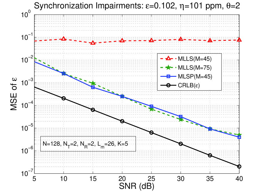
Figure 1: CRLB and MSE for the estimation of CFO.

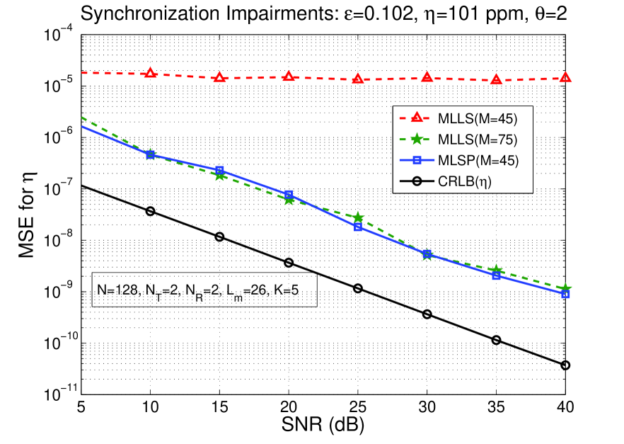
Figure 2: CRLB and MSE for the estimation of SFO.

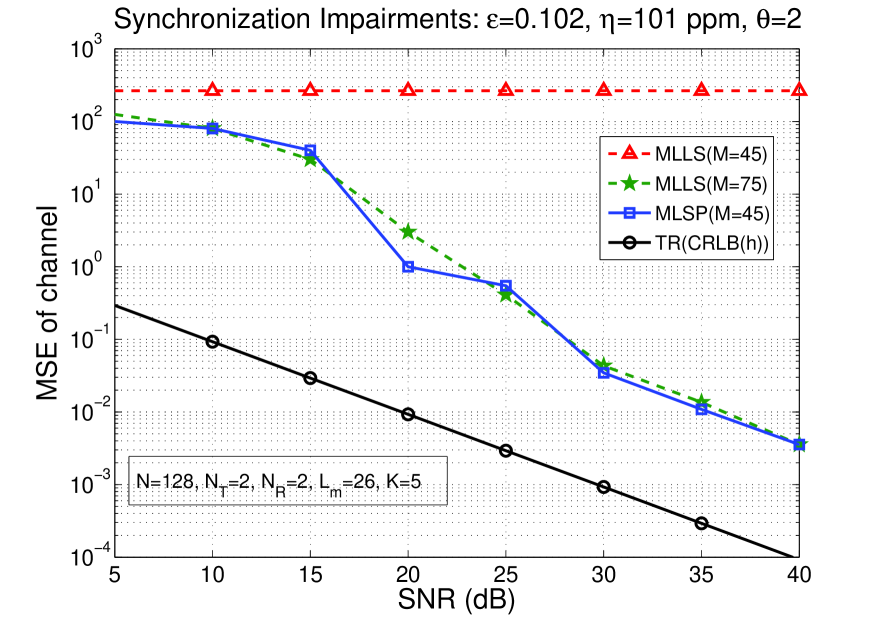
Figure 3: Tr(CRLB(h)) and MSE for the estimation of channel.

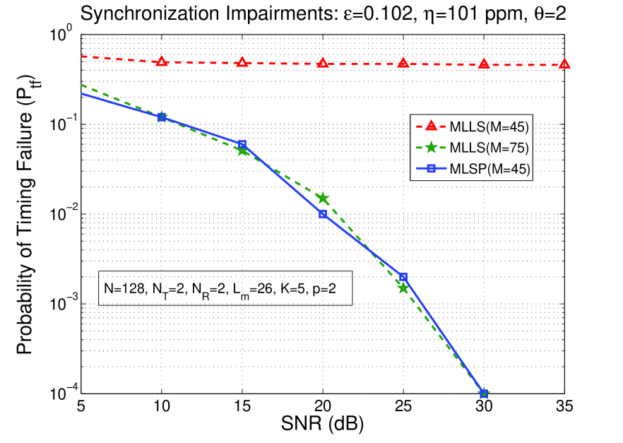
Figure 4: Probability of Timing Failure as a function of SNR(dB).

The Mean Square Error (MSE) values of the estimated parameters, using MLLS and MLSP, are calculated and are plotted in log-scale against SNR(dB), together with Cramér-Rao Lower Bound (CRLB) of the parameters [4], in Fig(1).- Fig(3). MLLS is simulated using MLSP algorithm given in Algorithm 2 by replacing the SP estimate of channel obtained in step 4 and step 5 using LS estimate of the channel. It is found from Fig(1).- Fig(3). that the MSE plots of MLLS for the estimation of CFO, SFO, and channel for $M$=$45$ fail, due to the poor performance of LS based estimation in under-determined system. Also, the MSE plots of MLSP for the estimation of CFO, SFO, and channel follow $\mathrm{CRLB}(\epsilon)$, $\mathrm{CRLB}(\eta)$, and $\mathrm{Tr}(\mathrm{CRLB}(\mathbf{h}))$ [4], respectively, but with a performance degradation of around $12$ dB, $13$ dB, and $15$ dB SNRs, respectively, at high SNR. The Probability of Timing Failure [4] for the estimation of $\theta$, defined as $\mathrm{P_{tf}}(p)=\mathrm{Pr}\left[|\hat{\theta}-\theta|\geqslant p\right]$, is calculated for $p$=$2$ and is plotted in Fig(4). for MLLS and MLSP, respectively. As in the cases of CFO, SFO, and channel, MLSP performs better than MLLS for the estimation of STE also. It is observed from the figures that, to have a comparable performance with MLSP using $90$ samples ($M$=$45$), MLLS requires at least $150$ samples ($M$=$75$), which shows the difference in computational complexity.

5 Conclusion

In this letter, we presented a low complexity ML joint estimation algorithm for single-user MIMO-OFDM system, where the received samples used for estimation are less than that required for an LS based ML estimation, MLLS. An ML algorithm for the joint estimation of synchronization impairments and channel using CS based technique, MLSP, is proposed. It is found from the simulations that MLSP performs better than MLLS for the joint estimation of CFO, SFO, STE, and channel.

References

• [1] Morelli M, Kuo C-CJ, Pun M-O. Synchronization Techniques for Orthogonal Frequency Division Multiple Access (OFDMA): A Tutorial Review. Proc. IEEE 2007;95(7):1394-427.
• [2] Nguyen-Le H, Le-Ngoc T, Ko C.C. Joint Channel Estimation and Synchronization for MIMO OFDM in the Presence of Carrier and Sampling Frequency Offsets. IEEE Trans. Veh. Technol. 2009;58(6):3075
• [3] Jose R, K.V.S. Hari. Joint Estimation of Synchronization Impairments in MIMO-OFDM System. Proceedings of National Conference on Communication, India, 2012.p.1-5.
• [4] Jose R, K.V.S. Hari. Maximum Likelihood Algorithms for Joint Estimation of Synchronization Impairments and Channel in MIMO-OFDM System. arXiv:1210.5314v2[cs.IT].
• [5] Donoho. Compressed Sensing. IEEE Trans. Inf. Theory 2006;52(4):1289 -306.
• [6] Candes EJ, Wakin MB. An Introduction to Compressive Sampling. IEEE Signal Processing Mag. 2008;25(2):21-30.
• [7] Wei D, Milenkovic O. Subspace Pursuit for Compressive Sensing Signal Reconstruction. IEEE Trans. Inf. Theory 2009;59(5):2230-49.