Analytic Treatment of Tipping Points for Social Consensus in Large Random Networks

Abstract

We introduce a homogeneous pair approximation to the Naming Game (NG) model by deriving a six-dimensional ODE for the two-word Naming Game. Our ODE reveals the change in dynamical behavior of the Naming Game as a function of the average degree $<k>$ of an uncorrelated network. This result is in good agreement with the numerical results. We also analyze the extended NG model that allows for presence of committed nodes and show that there is a shift of the tipping point for social consensus in sparse networks.

I Introduction

The dynamics of social influence has been heavily studied in the network science literature Schelling1978 ; Castellano2009 ; Kempe2003 . Some of the models used include the Voter Model vote , the threshold model Granovetter1978 , the Bass model Bass1969 and the Naming Game models Steels1995 ; Steels1998 ; Baronchelli2005 ; Baronchelli2006 . The last model is the focus of our paper. In this model, each node is assigned a list of names as its opinions chosen from an alphabet $S$. In each time step, two neighboring nodes, one listener and one speaker are randomly picked. The speaker randomly picks one name from its name list and sends it to the listener. If the name is not in the list of the listener, the listener will add this name to its list, otherwise the two communicators will achieve an agreement, i.e. both collapse their name list to this single name. The variations of this game can be classified as the “Original” (NG), “Listener Only” (LO-NG) and “Speaker Only” (SO-NG) types Baronchelli2 regarding the update when the communicators make an agreement, and as the “Direct”, “Reverse” and “Neutral” types regarding the way that the two communicators are randomly picked, as defined in DallAsta2006 . These variations have different behaviors but can be analyzed in the similar way. In this paper we mainly focus on the “Original” “Direct” version using binary alphabet of two symbols, denoted here as A and B.

A key feature in the Naming Game models (symmetric binary agreement version) is that once a susceptible individual adopts the new opinion, he can still revert back to his old opinion at all subsequent times which is suited to studying the dynamics of competing opinions where switching one’s opinion has little overhead, and where the opposing opinions A and B are not socially, culturally or morally ranked. These dynamics correspond to a particular case of the 2-convention NG introduced in Castellano2009 with the trust parameter $\beta=1$. Other versions of the Naming Games have been developed that address the issues of overall social preference of one opinion over the other through an asymmetry in the stickiness of each opinion.

Another significant difference between the Naming Games (NG) and other stochastic games on networks including population genetics models is the symmetric forms of the NG do not take into account the selective survivability or fitness of agents that adopt one opinion over another.

A third significant difference between the NG and other social influence models such as the Voter models vote is that in the NG, an agent is allowed to hold more than one opinions before switching to the other opinion. This changes the expected time to consensus starting from uniform initial conditions even in perfectly symmetric form of the models. Numerical studies in Castellano2009 have shown that for the symmetric NG on a complete graph, starting from the state where each agent has one of the two opinions with equal probability, the system first achieves consensus in order $\ln N$ number of time steps, as compared to order $N$ time steps for the Voter models. Here $N$ is the number of nodes in the network, and unit time consists of $N$ speaker-listener interactions.

Numerical studies in Castellano2009 have shown that for the symmetric NG on a complete graph, starting from the state where each node has one of the two opinions with equal probability, the number of time steps needed by the system to achieve consensus is of the order $\ln N$, while the number of time steps to consensus in the Voter models is of the order $N$. Here $N$ is the number of nodes in the network, and a single time step consists of $N$ speaker-listener interactions.

In this paper, we also address the nearly-symmetric cases of the Naming Game models where a single asymmetry is introduced into the models through the random inclusion of a minority fraction of committed agents whose opinion are fixed for all times to be A, say. The key observable is the expected time to consensus of the A opinion and its dependence on (I) the committed fraction and (II) the network topology.

In Zhang11 and Xie11 , we show that, for a complete graph, when the committed fraction grows beyond a critical value $p_{c}\approx 0.0979$, there is a super-exponential decrease in the time taken for the entire network to adopt the A opinion. Specifically, using a straight forward mean field approach, coarse-grained stochastic analysis, and direct simulations of the NG, we show that for $p<p_{c}$, the mean consensus time $T_{c}\sim e^{N}$, while for $p>p_{c}$, $T_{c}\sim\ln N$ . In the presence of committed agents of opinion $A$, the only absorbing state in the associated random walk Markov chain model Zhang11 is the consensus state of opinion $A$ while the near-consensus state where all susceptible agents have the $B$ opinion becomes a reflecting state. Similarly, the averaged or mean field system of two coupled nonlinear differential equations Xie11 , undergoes a saddle-node bifurcation when $p=p_{c}$, in which the saddle point (symmetric in phase plane in the case with no committed agents) merges with a node to form a new equilibrium point of saddle-node type Strogatzbook Golubitskybook . The $T_{c}\sim\ln N$ time scale comes from the slow dynamics along the center manifold between the saddle-node and the consensus of $A$ opinion, and is the same order as the symmetric case where there are no committed agents. In contrast, for $p<p_{c}$, the $T_{c}\sim e^{N}$ time scale is due to the additional numerous time steps spent along that portion of the center manifold which is between the stable fixed point and the saddle-point where the latter corresponds to a state with a larger fraction of agents of opinion $A$ than the former.

Simulations on a range of sparse random networks with 100 - 10000 nodes have shown, after extensive and costly numerical experiments, that the above tipping point effect of the NG with a minority fraction of committed agents is a very robust phenomenon with respect to underlying network topology. Of particular significance is the numerical / empirical observation Xie11 that as one lowers the average degree of the underlying random network, the tipping fraction $p_{c}$ decreases.

In this paper, we analytically establish the numerical discovery using a refined mean field approach Zhangcomple12 and report on precise changes in NG dynamics with respect to the average degree $<k>$ of an uncorrelated underlying network which are beyond the reach of the straight forward mean field model in Zhang11 , Xie11 . Specifically, the critical tipping fraction in the binary agreement model decreases to a minimum of 5 percent when the average degree $<k>=4$ from a maximum of 10 percent for complete graphs. This shows that the new mean field model is in better agreement with the numerical results reported above in Xie11 and provides a much improved approximation to NG dynamics on large random networks in comparison to the straight forward mean field model in Xie11 .

II Improved Mean Field Approach

Although the basic mean field approach applied to the NG models Xie11 have yielded significant results such as a phase transition at a critical fraction of the committed agents in the network, the tipping point Xie11 , its theoretical predictions deviate from the results of simulations on complex networks especially when the network is relatively “sparse”. The qualitative changes in dynamical behavior of the network under social games such as the NG, in terms of its average degree or the degree distribution, is important in network science, and we report here the significant results of a refined mean field model for the NG with committed agents.

Recently, a so-called homogeneous pair approximation has been introduced to study the dynamics of the voter model Vazquez Pugliese , a model simpler than the NG, which improves the basic mean field approximation by taking account of the correlation between the nearest neighbors. Their analysis is based on the master equation of the active links, the links between nodes with different opinions. Although it shows a spurious transition point, it captures most features of the dynamics and works very accurately on most uncorrelated networks such as Erdos-Renyi (ER) and scale-free (SF) networks.

In this paper, we apply a similarly improved mean field approach to the NG, especially the binary agreement model. Compared to the voter model, there are more than one type of active links (edges) in the NG, so we have to analyze all types of links including active and inert ones. As a consequence, instead of a one dimensional averaged nonlinear ODE in the voter model, we have a six dimensional nonlinear coupled system. We will derive the equations by analyzing all possible updates in the process and write it in a matrix form with the average degree $<k>$ as a explicit parameter. In contrast to the basic mean field theory, this improved ODE approximation clearly shows how the NG dynamics changes when $<k>$ decrease to 1, the critical value for ER network to have giant component, and converges to the basic mean field equations in Xie11 when $<k>$ grows to infinity. Next we show the significantly better agreement between the theoretical predictions of the new mean field theory and the simulations on ER network. Using this improved model, we are able to predict and replicate the empirically observed lowering of critical tipping fraction in low average degree networks, i.e. we need fewer committed agents to force a global consensus in a loosely connected social network.

III The Model

In the “Original” “Direct” version of Naming Game, every agent in the network has a naming list in its memory. In each time step, a speaker is randomly picked first and then a listener is randomly picked from the speaker’s neighbors (this order is called “Direct”). The speaker picks one name from its memory and sends it to the listener. If the listener does not know this name , it adds this new name to its list. Otherwise, both agents delete all names in their list but the one sent (this update is the “Original” version).

Consider the NG dynamics on an uncorrelated random network where the presence of links are independent, together with the following assumptions which comprise the foundation of the homogeneous pair approximation:

1. The opinions of direct neighbors are correlated, while there is no extra correlation besides that through the nearest neighbor. To make this assumption clear, suppose three nodes in the network are linked as 1-2-3 (so there is no link between 1 and 3). Their opinions are denoted by random variables $X_{1}$,$X_{2}$,$X_{3}$, correspondingly. Therefore our assumption says: $P(X_{1}|X_{2})\neq P(X_{1})$, but $P(X_{1}|X_{2},X_{3})=P(X_{1}|X_{2})$. This assumption is valid for all uncorrelated networks (Chung-Lu type network Chung , especially the ER network).

2. The opinion of a node and its degree are mutually independent. Suppose the node index $i$ is a random variable which labels a random node. In terms of the opinion and degree of node $i$, denoted respectively as $X_{i}$ and $k_{i}$, this assumption means $E[k_{i}|X_{i}]=<k>$, $P(X_{i}|k_{i})=P(X_{i})$ and $P(X_{i}|X_{j},k_{i},k_{j})=P(X_{i}|X_{j})$ where $j$ is a neighbor of $i$. This assumption is obviously satisfied for the networks in which every node has the same degree (regular geometry), but it is also valid for the network whose degree distribution is concentrated around its average (for example, Gaussian distribution with relatively small variance or Poisson distribution with not too small $<k>$). It can be shown that this assumption is good enough for ER network.

In other words, in typical mean field language, the probability distribution of the neighboring opinions of a specific node is an effective field. This field is however not uniform over the network but depends only on the opinion of the given node. For an uncorrelated random network with N nodes and average degree $<k>$, the number of links in this network is $M=N<k>/2$. We denote the numbers of nodes taking opinions A,B and AB as $n_{A}$, $n_{B}$, $n_{AB}$, their fractions as $p_{A}$,$p_{B}$, $p_{AB}$. We also denote the numbers of different types of links as $\vec{L}=[L_{A-A},L_{A-B},L_{A-AB},L_{B-B},L_{B-AB},L_{AB-AB}]^{T}$, and their fractions are given by $\vec{l}=\vec{L}/M$. We take $\vec{L}$ or $\vec{l}$ as the coarse grained macrostate vector. The global mean field is given by:

$$\vec{p}(\vec{L}) = \left(\begin{matrix}p_{A}\\ p_{B}\\ p_{AB}\\ \end{matrix}\right)={1\over 2M}\left(\begin{matrix}<k>n_{A}\\ <k>n_{B}\\ <k>n_{AB}\\ \end{matrix}\right)$$

$$= {1\over 2M}\left(\begin{matrix}2L_{A-A}+L_{A-B}+L_{A-AB}\\ L_{A-B}+2L_{B-B}+L_{B-AB}\\ L_{A-AB}+L_{B-AB}+2L_{AB-AB}\\ \end{matrix}\right).$$

Suppose $X_{i}$, $X_{j}$ are the opinions of two neighboring nodes. We simply write $P(X_{i}=A|X_{j}=B)$, for example, as $P(A|B)$. We also represent the effective fields for all these types of node in terms of $\vec{L}$:

$$\overrightarrow{P(\cdot|A)}(\vec{L})=\left(\begin{matrix}P(A|A)\\ P(B|A)\\ P(AB|A)\\ \end{matrix}\right)={1\over 2L_{A-A}+L_{A-B}+L_{A-AB}}\left(\begin{matrix}2L_{A-A}\\ L_{A-B}\\ L_{A-AB}\\ \end{matrix}\right),$$

$$\overrightarrow{P(\cdot|B)}(\vec{L})=\left(\begin{matrix}P(A|B)\\ P(B|B)\\ P(AB|B)\\ \end{matrix}\right)={1\over L_{A-B}+2L_{B-B}+L_{B-AB}}\left(\begin{matrix}L_{A-B}\\ 2L_{B-B}\\ L_{B-AB}\\ \end{matrix}\right),$$

$$\overrightarrow{P(\cdot|AB)}(\vec{L})=\left(\begin{matrix}P(A|AB)\\ P(B|AB)\\ P(AB|AB)\\ \end{matrix}\right)={1\over L_{A-AB}+L_{B-AB}+2L_{AB-AB}}\left(\begin{matrix}L_{A-AB}\\ L_{B-AB}\\ 2L_{AB-AB}\\ \end{matrix}\right).$$

To derive the averaged nonlinear ODE for NG dynamics, we calculate the expected change of $\vec{L}$ in one time step, $E[\Delta\vec{L}|\vec{L}]$. In the following equation, we add up the expectation $E[\Delta\vec{L}|\vec{L},\omega]$ conditioned by each type of nodes communications ($\omega$), and weighted by the probability of this type of nodes communications, $P(\omega)$.

$$E[\Delta\vec{L}|\vec{L}]=\sum_{\omega}P(\omega)E[\Delta\vec{L}|\vec{L},\omega].$$ (1)

For brevity, we display the calculation of one term in the above summation as example. Consider the case: listener holds opinion A while speaker has opinion B, and denote this case by $\omega=(B\rightarrow A)$. The probability for this type of communication is

$$P(B\rightarrow A)=p_{B}P(A|B)={1\over 2M}L_{A-B}.$$

The direct consequence of this communication is that the link between the listener and speaker changes from A-B into AB-B, so $L_{A-B}$ decreases by 1 and $L_{B-AB}$ increases by 1. This direct change of $\vec{L}$ is represented by

$$\vec{D}(B\rightarrow A)=\left(\begin{array}[]{c}0\\ -1\\ 0\\ 0\\ 1\\ 0\\ \end{array}\right).$$

Furthermore, since the listener changes opinions from A to AB, all his other related links change. The number of these links is on average $<k>-1$ (here we use the assumption 2, $E[k_{i}|X_{i}]=<k>$.). The probabilities for each link to be A-A, A-B, A-AB before the communication is given by $\overrightarrow{P(\cdot|A)}$ (here we use assumption 1). After the communication, these links will change into AB-A, AB-B, AB-AB correspondingly. This related change of $\vec{L}$ is represented by

$$(<k>-1)\left(\begin{array}[]{ccc}-1&0&0\\ 0&-1&0\\ 1&0&-1\\ 0&0&0\\ 0&1&0\\ 0&0&1\\ \end{array}\right)\left(\begin{array}[]{c}P(A|A)\\ P(B|A)\\ P(AB|A)\\ \end{array}\right).$$

The 6-by-3 matrix in the above expression indicates the link correspondence between A-A, A-B, A-AB and AB-A, AB-B, AB-AB when a “A node” changes into “AB node”, we denote it by

$$Q_{A}=\left(\begin{array}[]{ccc}-1&0&0\\ 0&-1&0\\ 1&0&-1\\ 0&0&0\\ 0&1&0\\ 0&0&1\\ \end{array}\right).$$

Let $\vec{R}(B\rightarrow A)=Q_{A}\overrightarrow{P(\cdot|A)}$, we obtain:

$$E[\Delta\vec{L}|\vec{L},B\rightarrow A]=\vec{D}(B\rightarrow A)+(<k>-1)\vec{R}(B\rightarrow A).$$

On the right hand side of the above equation, the first term represents the direct change and the second term represents the related change.

Similarly, we analyze all the other terms in equation (1) for different $\omega$ (the listener and speaker’s opinions), and write the weighted sum in matrix form, we obtain:

$$E[\Delta\vec{L}|\vec{L}]={1\over M}\left[D+(<k>-1)R\right]\vec{L},$$

where $D$ is a constant matrix whose column vectors come from linear combinations of $\vec{D}(\omega)$’s:

$$D=\left(\begin{array}[]{cccccc}0&0&{3\over 4}&0&0&{1\over 2}\\ 0&-1&0&0&0&0\\ 0&{1\over 2}&-1&0&0&0\\ 0&0&0&0&{3\over 4}&{1\over 2}\\ 0&{1\over 2}&0&0&-1&0\\ 0&0&{1\over 4}&0&{1\over 4}&-1\\ \end{array}\right),$$

and matrix $R$ is a function of $\vec{L}$, given by column vectors which come from $\vec{R}(\omega)$’s:

$$R=\big{(}\vec{0},{1\over 2}[Q_{A}\overrightarrow{P(\cdot|A)}+Q_{B}\overrightarrow{P(\cdot|B)}],Q_{A}[{1\over 4}\overrightarrow{P(\cdot|A)}-{3\over 4}\overrightarrow{P(\cdot|AB)}],$$

$$\vec{0},Q_{B}[{1\over 4}\overrightarrow{P(\cdot|B)}-{3\over 4}\overrightarrow{P(\cdot|AB)}],-(Q_{A}+Q_{B})\overrightarrow{P(\cdot|AB)}\big{)}.$$

Here $Q_{B}$, similar to $Q_{A}$ defined above, indicates the link correspondence between B-A, B-B, B-AB and AB-A, AB-B, AB-AB when a “B node” changes into “AB”,

$$\ Q_{B}=\left(\begin{array}[]{ccc}0&0&0\\ -1&0&0\\ 1&0&0\\ 0&-1&0\\ 0&1&-1\\ 0&0&1\\ \end{array}\right).$$

When “AB node” changes into “A” or “B”, the link correspondence is given by $-Q_{A}$ or $-Q_{B}$ respectively.

Then we normalize $\vec{L}$ by the total number of links $M$ and normalize time by the number of nodes $N$ to obtain:

$${d\over dt}\vec{l} = {N\over M}E[\Delta\vec{L}|\vec{L}]={N\over M}\left[D+(<k>-1)R\right]\vec{l}$$ (2)

$$= 2\left[{1\over<k>}D+({<k>-1\over<k>})R\right]\vec{l}.$$

Thus, we derived the new mean field ODEs for $\vec{l}$ and the average degree $<k>$ of the underlying social network on which the NG is played is explicit in the formula. In the last line, the first term is linear and comes from the direct change of the link between the listener and the speaker. The second term is nonlinear and comes from the related changes.

Under the previous basic mean field assumptions in Xie11 , the first term does not exist because there is no specific “speaker” and every one receives messages from the effective mean field. When $<k>\rightarrow 1$, the new ODE becomes:

$${d\over dt}\vec{l}=2D\vec{l},$$

which is a linear system. When $<k>\rightarrow\infty$, this ODE becomes:

$${d\over dt}\vec{l}=2R\vec{l}.$$

If in matrix $R$ we further require $\overrightarrow{P(\cdot|A)}=\overrightarrow{P(\cdot|B)}=\overrightarrow{P(\cdot|AB)}=\vec{p}$ and transform the coordinates by $\vec{L}\rightarrow\vec{p}(\vec{L})$, this ODE reverts to the one we have under the basic mean field assumption in Xie11 .

IV Numerical Results without committed agents

In this section, we show the numerical results of solving our ODEs by Runge-Kutta method and compare the phase trajectories with those of the basic mean field theory and also with the stochastic dynamical trajectories of the simulated NG on random networks of varying average degree. Fig.1 shows the comparison between our theoretical prediction (color lines) and the simulation on ER networks (black solid lines). The dotted lines are theoretical prediction by basic mean field approximation. We calculate the evolution of the fractions of nodes with A, B and AB opinions respectively and show that the prediction of the older basic mean field approximation deviates from the simulations significantly while that of the homogeneous pair approximation matches simulations very well.

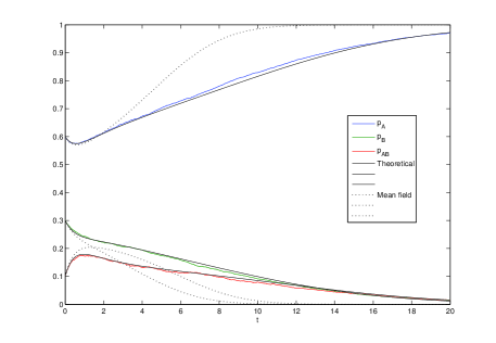
Figure 1: Fractions of A, B and AB nodes as function of time. The three color lines are the averages of 50 runs of NG (without committed agents) on ER network with $N=500$ and $<k>=5$. The black solid lines are solved from the ODE above with the same $<k>$. The black dotted lines are from the ODE using mean field assumption.

Fig.2 shows the trajectories of the macrostate mapped onto two dimensional space ($p_{A}$,$p_{B}$), the black line is the trajectory predicted by the mean field approximation. We find that when $<k>$ is large enough, say $50$, the homogeneous pair approximation is very close to the mean field approximation. When $<k>$ decreases, the trajectory tends to the line $p_{AB}=1-p_{A}-p_{B}=0$, which means there are fewer nodes with mixed opinions than predicted by the mean field. In this situation, opinions of neighbors are highly correlated forming the “opinion blocks”, and mixed opinion (AB) nodes can only appear on the boundary between the “A opinion block” and “B opinion block”.

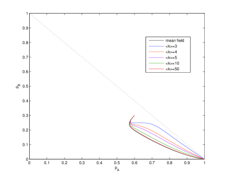
Figure 2: The trajectories of NG (no committed agents)solved from the ODE with different $<k>$ mapped onto 2D macrostate space. When $<k>\rightarrow\infty$, the trajectory tends to that of the mean field equation. When $<k>\rightarrow 1$, the trajectory get close to the line $p_{AB}=1-p_{A}-p_{B}=0$.

In the ODE models, it is hard to identify a proper cutoff for “total consensus”. Therefore, to make a comparison between the theoretical prediction and the simulation, we consider $\eta$-consensus ($T_{\eta}$) which is the first time $p_{A}$ or $p_{B}$ achieves $\eta$. Fig.3 shows the comparison of $T_{\eta}$ ($\eta=0.95$) for different system size $N$ and average degrees $<k>$. According to this figure, we find that when $N$ grows, the relative standard deviation of $T_{0.95}$ ($\Delta T_{0.95}/T_{0.95}\approx\Delta\ln(T_{0.95})$) decreases, which validates the pair approximation in the sense of thermodynamic limit. Further more, when $<k>$ grows, the pair approximation tends to the simple mean field assumption.

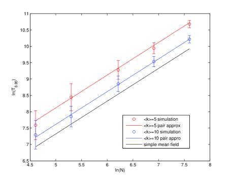
Figure 3: Comparison of $\eta$-consensus times $T_{0.95}$ of NG (no committed agent) between the simulation and theoretical prediction for different system sizes $N$ and average degrees $<k>$. The straight lines are from theoretical analysis under simple mean field assumption or pair approximation. The cycles and error bars show the means and the relative standard deviations of $T_{0.95}$ by simulation of dynamics

V Committed Agents

In this section, we consider the asymmetric case of the NG on large random networks with $p$ (fraction) committed agents (nodes that never change their opinions) of opinion A. Initially, all the other nodes are of opinion B. The main question considered here is under what conditions it is possible for the committed nodes to persuade the others and achieve a global consensus. Previous studies found there is a robust critical value of $p$ called the tipping point. Above this value, it is possible and the persuasion takes a short time, while below this value, it is nearly impossible as it takes exponentially long time with respect to the system sizesXie11 ; Zhang11 .

Similar to what we did in the previous section, we derive the new mean field ODE for the macrostate in the NG with committed agents, although the macrostate now contains three more dimensions. $\vec{L}=[L_{A-C},L_{B-C},L_{AB-C},L_{A-A},L_{A-B},L_{A-AB},L_{B-B},L_{B-AB},L_{AB-AB}]^{T}$, where $C$ denotes the committed A opinion and $A$ itself denotes the non-committed one. Hence we have a nine dimensional ODE which has the same form as equation (2), but with different details in $D$ and $R$ given below:

$$D=\left(\begin{array}[]{ccccccccc}0&0&{3\over 4}&0&0&0&0&0&0\\ 0&-{1\over 2}&0&0&0&0&0&0&0\\ 0&{1\over 2}&-{3\over 4}&0&0&0&0&0&0\\ 0&0&0&0&0&{3\over 4}&0&0&{1\over 2}\\ 0&0&0&0&-1&0&0&0&0\\ 0&0&0&0&{1\over 2}&-1&0&0&0\\ 0&0&0&0&0&0&0&{3\over 4}&{1\over 2}\\ 0&0&0&0&{1\over 2}&0&0&-1&0\\ 0&0&0&0&0&{1\over 4}&0&{1\over 4}&-1\\ \end{array}\right),$$

$$Q_{A}=\left(\begin{array}[]{cccc}-1&0&0&0\\ 0&0&0&0\\ 1&0&0&0\\ 0&-1&0&0\\ 0&0&-1&0\\ 0&1&0&-1\\ 0&0&0&0\\ 0&0&1&0\\ 0&0&0&1\\ \end{array}\right),\ \ Q_{B}=\left(\begin{array}[]{cccc}0&0&0&0\\ -1&0&0&0\\ 1&0&0&0\\ 0&0&0&0\\ 0&-1&0&0\\ 0&1&0&0\\ 0&0&-1&0\\ 0&0&1&-1\\ 0&0&0&1\\ \end{array}\right),$$

$$R = (\vec{0},{1\over 2}Q_{B}\overrightarrow{P(\cdot|B)},-{3\over 4}Q_{A}\overrightarrow{P(\cdot|AB)},\vec{0},{1\over 2}[Q_{A}\overrightarrow{P(\cdot|A)}+Q_{B}\overrightarrow{P(\cdot|B)}],$$

$$Q_{A}[{1\over 4}\overrightarrow{P(\cdot|A)}-{3\over 4}\overrightarrow{P(\cdot|AB)}],\vec{0},Q_{B}[{1\over 4}\overrightarrow{P(\cdot|B)}-{3\over 4}\overrightarrow{P(\cdot|AB)}],$$

$$-(Q_{A}+Q_{B})\overrightarrow{P(\cdot|AB)}).$$

Finally, we show the change of the critical tipping fraction with respect to the average degree $<k>$ of the underlying random networks in Fig.4. Starting from the state that $p_{B}=1-p$, the new ODE system will go to a stable state for which $p_{B}=p_{B}^{*}$. $p_{B}^{*}$ is $0$ if the committed agents finally achieve the global consensus. The sharp drop of each curve indicates the tipping point transition with the corresponding $<k>$. Fig.5 shows the normalized consensus time, $T_{0.95}/N$ around the tipping point $p_{c}$ for different system sizes. When $p>p_{c}$, $T_{0.95}/N$ is logarithmic with $N$; when $p<p_{c}$, $T_{0.95}/N$ grows very fast (since it takes to much time, we stop the simulation when $T_{0.95}/N$ exceeds $10^{4}$). Fig.5 confirms the tipping point found in Fig.4 is consistent with the transition point between the region of the logarithmic consensus time and exponential consensus time, and when the system size grows, the transition becomes sharper.

According to Fig.4, the tipping point shifts left when the average degree $<k>$ decreases. This theoretical result confirms and replicate in full without costly numerical simulations, the observed lowering of the tipping fraction as a function of decreasing the average degree of the underlying large random networks.

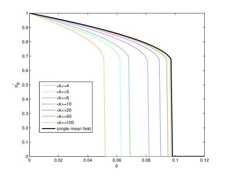
Figure 4: Fraction of B nodes of the stable point ($p_{B}^{*}$) as a function of the fraction of nodes committed to A (p). The color lines consist of stable points obtained by tracking the ODE of NG on ER for a long enough time. The black lines are the stable points solved from the mean field ODE.

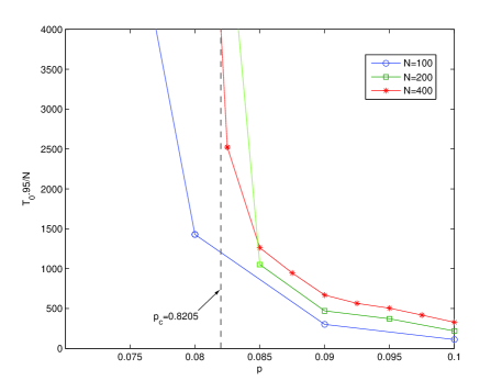
Figure 5: Normalized consensus time, $T_{0.95}/N$ around the tipping point $p_{c}=0.8205$ (vertical dash line) when $<k>=10$. Each data point is obtained by average of 100 runs of NG simulation with committed agents on ER network. The simulation stops when $T_{0.95}/N$ exceed $10^{4}$, since it almost never achieve consensus when $p<p_{c}$.

- (1) Thomas Schelling Micromotives and Macrobehavior. Norton (1978).
- (2) C. Castellano, S. Fortunato and V. Loreto: Statistical physics of social dynamics. Reviews of Modern Physics, 81(2):591-646 (2009).
- (3) D. Kempe, J. Kleinberg, E. Tardos. Maximizing the Spread of Influence through a Social Network. Proc. 9th ACM SIGKDD Intl. Conf. on Knowledge Discovery and Data Mining, (2003).
- (4) P. Clifford and A. Sudbury: ”A Model for Spatial Conflict”. Biometrika 60 (3): 581 C588 (1973).
- (5) M. Granovetter : Threshold Models of Collective Behavior. American Journal of Sociology 83 (6): 1420 C1443 (1978).
- (6) F. Bass : A new product growth model for consumer durables. Management Science 15 (5): p215 C227 (1969).
- (7) L. Steels: A self-organizing spatial vocabulary. Artificial Life, 2(3):319-332 (1995).
- (8) L. Steels and A. MacIntyre: Spatially distributed naming games. Advances in complex systems, 1: 301-324 (1998)
- (9) A. Baronchelli, L. Dall’Asta, A. Barrat and V. Loreto: Topology Induced Coarsening in Language Games. Physical Review E, 73:015102 (2005).
- (10) A. Baronchelli, M. Felici, V. Loreto, E. Caglioti and L. Steel: Sharp transition towards shared vocabularites in multi-agent system. J. Stat. Mech.: Theory Exp. P06014 (2006)
- (11) A. Baronchelli: Role of feedback and broadcasting in the naming game. Phys. Rev. E 83,046103 (2011).
- (12) Luca Dall Asta, Andrea Baronchelli, Alain Barrat and Vittorio Loreto: “Nonequilibrium dynamics of language games on complex networks” Phys. Rev. E 74, 036105 (2006).
- (13) W. Zhang, C. Lim, S. Sreenivasan, J. Xie, B. K. Szymanski, and G. Korniss: Social influencing and associated random walk models: Asymptotic consensus times on the complete graph Chaos 21, 2, 025115 (2011).
- (14) J. Xie, S. Sreenivasan, G. Korniss, W. Zhang, C. Lim, B. K. Szymanski: Social Consensus through the Influence of Committed Minorities, Phys. Rev. E 84, 011130 (2011).
- (15) S. H. Strogatz: Nonlinear Dynamics And Chaos: With Applications To Physics, Biology, Chemistry, And Engineering. Da Capo Press, (1994).
- (16) M. Golubitsky, D. G. Schaeffer, I. Stewart: Singularities and groups in bifurcation theory, Volume 2. Springer, (1988).
- (17) W. Zhang, C. Lim, G. Korniss, B. Szymanski, S. Sreenivasan and J. Xie: Tipping Points of Diehards in Social Consensus on Large Random Networks. Proc. 3rd Workshop on Complex Networks, CompleNet, Melbourne, FL, March 7-9, 2012.
- (18) F. Vazquez and V. M. Egu luz: Analytical solution of the voter model on uncorrelated networks. New Journal of Physics 10, 063011 (2008).
- (19) E. Pugliese and C. Castellano: Heterogeneous pair approximation for voter models on networks. Eur. Lett. 88, 5, pp. 58004 (2009).
- (20) F. Chung and L. Lu: The Average Distances in Random Graphs with Given Expected Degrees. Proceeding of National Academy of Science 99,15879 C15882 (2002).