Bingham Procrustean Alignment for Object Detection in Clutter

Abstract

A new system for object detection in cluttered RGB-D images is presented. Our main contribution is a new method called Bingham Procrustean Alignment (BPA) to align models with the scene. BPA uses point correspondences between oriented features to derive a probability distribution over possible model poses. The orientation component of this distribution, conditioned on the position, is shown to be a Bingham distribution. This result also applies to the classic problem of least-squares alignment of point sets, when point features are orientation-less, and gives a principled, probabilistic way to measure pose uncertainty in the rigid alignment problem. Our detection system leverages BPA to achieve more reliable object detections in clutter.

I Introduction

Detecting known, rigid objects in RGB-D images relies on being able to align 3-D object models with an observed scene. If alignments are inconsistent or inaccurate, detection rates will suffer. In noisy and cluttered scenes (such as shown in figure 1), good alignments must rely on multiple cues, such as 3-D point positions, surface normals, curvature directions, edges, and image features. Yet there is no existing alignment method (other than brute force optimization) that can fuse all of this information together in a meaningful way.

The Bingham distribution has recently been shown to be useful for fusing orientation information for 3-D object detection [6]. In this paper, we derive a surprising result connecting the Bingham distribution to the classical least-squares alignment problem, which allows our new system to easily fuse information from both position and orientation information in a principled, Bayesian alignment system which we call Bingham Procrustean Alignment (BPA).

I-A Background

Rigid alignment of two 3-D point sets $X$ and $Y$ is a well-studied problem—one seeks an optimal (quaternion) rotation ${\bf q}$ and translation vector ${\bf t}$ to minimize an alignment cost function, such as sum of squared errors between corresponding points on $X$ and $Y$. Given known correspondences, ${\bf t}$ and ${\bf q}$ can be found in closed form with Horn’s method [8]. If correspondences are unknown, the alignment cost function can be specified in terms of sum-of-squared distances between nearest-neighbor points on $X$ and $Y$, and iterative algorithms like ICP (Iterative Closest Point) are guaranteed to reach a local minimum of the cost function [4]. During each iteration of ICP, Horn’s method is used to solve for an optimal ${\bf t}$ and ${\bf q}$ given a current set of correspondences, and then the correspondences are updated using nearest neighbors given the new pose.

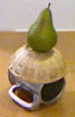
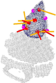
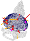
Figure 1: Object detections found with our system, along with the feature correspondences that BPA used to align the model. Surface features are indicated by red points, with lines sticking out of them to indicate orientations (red for normals, orange for principal curvatures). Edge features (which are orientation-less) are shown by magenta points.

ICP can be slow, because it needs to find dense correspondences between the two point sets at each iteration. Sub-sampling the point sets can improve speed, but only at the cost of accuracy when the data is noisy. Another drawback is its sensitivity to outliers—for example when it is applied to a cluttered scene with segmentation error.

Particularly because of the clutter problem, many modern approaches to alignment use sparse point sets, where one only uses points computed at especially unique keypoints in the scene. These keypoint features can be computed from either 2-D (image) or 3-D (geometry) information, and often include not only positions, but also orientations derived from image gradients, surface normals, principal curvatures, etc. However, these orientations are typically only used in the feature matching and pose clustering stages, and are ignored during the alignment step.

Another limitation is that the resulting alignments are often based on just a few features, with noisy position measurements, and yet there is very little work on estimating confidence intervals on the resulting alignments. This is especially difficult when the features have different noise models—for example, a feature found on a flat surface will have a good estimate of its surface normal, but a high variance principal curvature direction, while a feature on an object edge may have a noisy normal, but precise principal curvature. Ideally, we would like to have a posterior distribution over the space of possible alignments, given the data, and we would like that distribution to include information from feature positions and orientation measurements, given varying noise models.

As we will see in the next section, a full joint distribution on ${\bf t}$ and ${\bf q}$ is difficult to obtain. However, in the original least-squares formulation, it is possible to solve for the optimal ${\bf t}^{*}$ independently of ${\bf q}^{*}$, simply by taking ${\bf t}^{*}$ to be the translation which aligns the centroids of $X$ and $Y$. Given a fixed ${\bf t}^{*}$, solving for the optimal ${\bf q}^{*}$ then becomes tractable. In a Bayesian analysis of the least-squares alignment problem, we seek a full distribution on ${\bf q}$ given ${\bf t}$, not just the optimal value, ${\bf q}^{*}$. That way we can assess the confidence of our orientation estimates, and fuse $p({\bf q}|{\bf t})$ with other sources of orientation information, such as from surface normals.

Remarkably, given the common assumption of independent, isotropic Gaussian noise on position measurements (which is implicit in the classical least-squares formulation), we can show that $p({\bf q}|{\bf t})$ is a Bingham distribution. This result makes it easy to combine the least-squares distribution on ${\bf q}|{\bf t}$ with other Bingham distributions from feature orientations (or prior distributions), since the Bingham is a common distribution for encoding uncertainty on 3-D rotations represented as unit quaternions [5, 6, 2].

The mode of the least-squares Bingham distribution on ${\bf q}|{\bf t}$ will be exactly the same as the optimal orientation ${\bf q}^{*}$ from Horn’s method. When other sources of orientation information are available, they may bias the distribution away from ${\bf q}^{*}$. Thus, it is important that the concentration (inverse variance) parameters of the Bingham distributions are accurately estimated for each source of orientation information, so that this bias is proportional to confidence in the measurements. (See the appendix for an example.)

We use our new alignment method, BPA, to build an object detection system for known, rigid objects in cluttered RGB-D images. Our system combines information from surface and edge feature correspondences to improve object alignments in cluttered scenes (as shown in figure 1), and acheives state-of-the-art recognition performance on both an existing Kinect data set [1], and on a new data set containing far more clutter and pose variability than any existing data set.

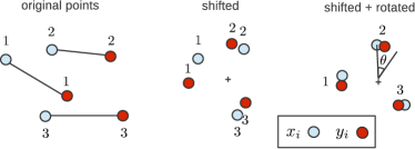
Figure 2: Rigid alignment of two point sets.

II Bingham Procrustean Alignment

Given two 3-D point sets $X$ and $Y$ in one-to-one correspondence, we seek a distribution over the set of rigid transformations of $X$, parameterized by a (quaternion) rotation ${\bf q}$ and a translation vector ${\bf t}$. Assuming independent Gaussian noise models on deviations between corresponding points on $Y$ and (transformed) $X$, the conditional distribution $p({\bf q}|{\bf t},X,Y)$ is proportional to $p(X,Y|{\bf q},{\bf t})p({\bf q}|{\bf t})$, where

$$p(X,Y|{\bf q},{\bf t}) =\prod_{i}p({\bf x_{i}},{\bf y_{i}}|{\bf q},{\bf t})$$ (1)

$$=\prod_{i}N(Q({\bf x_{i}}+{\bf t})-{\bf y_{i}};{\bf 0},\Sigma_{i})$$ (2)

given that $Q$ is ${\bf q}$’s rotation matrix, and covariances $\Sigma_{i}$.

Given isotropic noise models on point deviations (so that $\Sigma_{i}$ is a scalar times the identity matrix), $p({\bf x_{i}},{\bf y_{i}}|{\bf q},{\bf t})$ reduces to a 1-D Gaussian PDF on the distance between ${\bf y_{i}}$ and $Q({\bf x_{i}}+{\bf t})$, yielding

$$p({\bf x_{i}},{\bf y_{i}}|{\bf q},{\bf t}) =N(\|Q({\bf x_{i}}+{\bf t})-{\bf y_{i}}\|;0,\sigma_{i})$$

$$=N(d_{i};0,\sigma_{i})$$

where $d_{i}$ depends on ${\bf q}$ and ${\bf t}$.

Now consider the triangle formed by the origin (center of rotation), $Q({\bf x_{i}}+{\bf t})$ and ${\bf y_{i}}$, as shown on the left of figure 3. By the law of cosines, the squared-distance between $Q({\bf x_{i}}+{\bf t})$, and ${\bf y_{i}}$ is $d^{2}=a^{2}+b^{2}-ab\cos(\theta)$, which only depends on ${\bf q}$ via the angle $\theta$ between the vectors $Q({\bf x_{i}}+{\bf t})$ and ${\bf y_{i}}$. (We drop the $i$-subscripts on $d$, $a$, $b$, and $\theta$ for brevity.) We can thus replace $p({\bf x_{i}},{\bf y_{i}}|{\bf q},{\bf t})$ with

$$p({\bf x_{i}},{\bf y_{i}}|\theta,{\bf t})=\frac{1}{Z}\exp\left\{\frac{ab\cos(\theta)}{\sigma^{2}}\right\}$$ (3)

which has the form of a Von-Mises distribution on $\theta$.

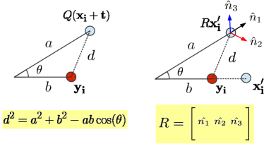
Figure 3: Distance between corresponding points as a function of orientation.

Next, we need to demonstrate how $\theta$ depends on ${\bf q}$. Without loss of generality, assume that ${\bf y_{i}}$ points along the axis $(1,0,0)$. When this is not the case, the Bingham distribution over ${\bf q}$ which we derive below can be post-rotated by any quaternion which takes $(1,0,0)$ to ${\bf y_{i}}/\|{\bf y_{i}}\|$.

Clearly, there will be a family of ${\bf q}$’s which rotate ${\bf x_{i}}+{\bf t}$ to form an angle of $\theta$ with ${\bf y_{i}}$, since we can compose ${\bf q}$ with any rotation about ${\bf x_{i}}+{\bf t}$ and the resulting angle with ${\bf y_{i}}$ will still be $\theta$. To demonstrate what this family is, we first let ${\bf s}$ be a unit quaternion which rotates ${\bf x_{i}}+{\bf t}$ onto ${\bf y_{i}}$’s axis, and let ${\bf x^{\prime}_{i}}=S({\bf x_{i}}+{\bf t})$, where $S$ is ${\bf s}$’s rotation matrix. Then, let ${\bf r}$ (with rotation matrix $R$) be a quaternion that rotates ${\bf x^{\prime}_{i}}$ to $Q({\bf x_{i}}+{\bf t})$, so that ${\bf q}={\bf r}\circ{\bf s}$. Because ${\bf y_{i}}$ and ${\bf x^{\prime}_{i}}$ point along the axis $(1,0,0)$, the first column of $R$, $\hat{n_{1}}$, will point in the direction of $Q({\bf x_{i}}+{\bf t})$, and form an angle of $\theta$ with ${\bf y_{i}}$, as shown on the right side of figure 3. Thus, $\hat{n_{1}}\cdot(1,0,0)=\hat{n_{11}}=\cos\theta$.

The rotation matrix of quaternion ${\bf r}=(r_{1},r_{2},r_{3},r_{4})$ is

$$R=\biggl{[}\begin{smallmatrix}r_{1}^{2}+r_{2}^{2}-r_{3}^{2}-r_{4}^{2}&\;\;&2r_{2}r_{3}-2r_{1}r_{4}&\;\;&2r_{2}r_{4}+2r_{1}r_{3}\\ 2r_{2}r_{3}+2r_{1}r_{4}&&r_{1}^{2}-r_{2}^{2}+r_{3}^{2}-r_{4}^{2}&&2r_{3}r_{4}-2r_{1}r_{2}\\ 2r_{2}r_{4}-2r_{1}r_{3}&&2r_{3}r_{4}+2r_{1}r_{2}&&r_{1}^{2}-r_{2}^{2}-r_{3}^{2}+r_{4}^{2}\end{smallmatrix}\biggr{]}$$

Therefore, $\cos\theta=\hat{n_{11}}=r_{1}^{2}+r_{2}^{2}-r_{3}^{2}-r_{4}^{2}=1-2r_{3}^{2}-2r_{4}^{2}$.

We can now make the following claim about $p({\bf x_{i}},{\bf y_{i}}|{\bf q},{\bf t})$:

Claim 1.

Given that ${\bf y_{i}}$ lies along the $(1,0,0)$ axis, then the probability density $p({\bf x_{i}},{\bf y_{i}}|{\bf q},{\bf t})$ is proportional to a Bingham density on ${\bf q}$ with parameters

$$\Lambda=(-\frac{2ab}{\sigma^{2}},-\frac{2ab}{\sigma^{2}},0)\;\;\;\;\textrm{and}\;\;\;\;V=\biggl{[}\begin{smallmatrix}0&0&0\\ 0&0&1\\ 1&0&0\\ 0&1&0\end{smallmatrix}\biggr{]}\circ{\bf s}=W\circ{\bf s}\;\;\;,$$

where “$\circ$” indicates column-wise quaternion multiplication.

Proof.

The Bingham density in claim 1 is given by

$$p({\bf q}|\Lambda,V) =\frac{1}{F}\exp\sum_{j=1}^{3}\lambda_{j}(({\bf w_{j}}\circ{\bf s})^{T}{\bf q})^{2}$$ (4)

$$=\frac{1}{F}\exp\left\{-\frac{2ab}{\sigma^{2}}r_{3}^{2}-\frac{2ab}{\sigma^{2}}r_{4}^{2}\right\}$$ (5)

$$=\frac{1}{F^{\prime}}\exp\left\{\frac{ab\cos\theta}{\sigma^{2}}\right\}$$ (6)

since $({\bf w_{j}}\circ{\bf s})^{T}{\bf q}={\bf w_{j}}^{T}({\bf q}\circ{\bf s^{-1}})={\bf w_{j}}^{T}{\bf r}$, and $\cos\theta=1-2r_{3}^{2}-2r_{4}^{2}$. Since (6) is proportional to (3), we conclude that $p({\bf q}|\Lambda,V)\propto p({\bf x_{i}},{\bf y_{i}}|{\bf q},{\bf t})$, as claimed.

∎

Claim 2.

Let ${\bf s^{\prime}}$ be a quaternion that rotates $(1,0,0)$ onto the axis of ${\bf y_{i}}$ (for arbitrary ${\bf y_{i}}$). Then the probability density $p({\bf x_{i}},{\bf y_{i}}|{\bf q},{\bf t})$ is proportional to a Bingham density on ${\bf q}$ with parameters

$$\Lambda=(-\frac{2ab}{\sigma^{2}},-\frac{2ab}{\sigma^{2}},0)\;\;\;\;\textrm{and}\;\;\;\;V={\bf s^{\prime}}\circ\biggl{[}\begin{smallmatrix}0&0&0\\ 0&0&1\\ 1&0&0\\ 0&1&0\end{smallmatrix}\biggr{]}\circ{\bf s}\;\;\;,$$

where “$\circ$” indicates column-wise quaternion multiplication.

As explained above, the distribution on ${\bf q}$ from claim 1 must simply be post-rotated by ${\bf s^{\prime}}$ when ${\bf y_{i}}$ is not aligned with the $(1,0,0)$ axis. The proof is left to the reader. Putting it all together, we find that

$$p({\bf q}|{\bf t},X,Y) \propto\prod_{i}{\rm Bingham}({\bf q};\Lambda_{i},V_{i})\cdot p({\bf q}|{\bf t})$$ (7)

$$={\rm Bingham}({\bf q};\tilde{\Lambda},\tilde{V})\cdot p({\bf q}|{\bf t})$$ (8)

where $\Lambda_{i}$ and $V_{i}$ are taken from claim 2, and where $\tilde{\Lambda}$ and $\tilde{V}$ are computed from the formula for multiplication of Bingham PDFs, which is given in the appendix.

Equation 8 tells us that, in order to update a prior on ${\bf q}$ given ${\bf t}$ after data points $X$ and $Y$ are observed, one must simply multiply the prior by an appropriate Bingham term. Therefore, assuming a Bingham prior over ${\bf q}$ given ${\bf t}$ (which includes the uniform distribution), the conditional posterior, $p({\bf q}|{\bf t},X,Y)$ is the PDF of a Bingham distribution.

To demonstrate this fact, we relied only upon the assumption of independent isotropic Gaussian noise on position measurements, which is exactly the same assumption made implicitly in the least-squares formulation of the optimal alignment problem. This illustrates a deep and hitherto unknown connection between least-squares alignment and the Bingham distribution, and paves the way for the fusion of orientation and position measurements in a wide variety of applications.

II-A Incorporating Orientation Measurements

Now that we have shown how the orientation information from the least-squares alignment of two point sets $X$ and $Y$ is encoded as a Bingham distribution, it becomes trivial to incorporate independent orientation measurements at some or all of the points, provided that the orientation noise model is Bingham. Given orientation measurements $(O_{X},O_{Y})$,

$$p({\bf q}|{\bf t},X, Y,O_{X},O_{Y})$$

$$\propto p(X,Y,O_{X},O_{Y}|{\bf q},{\bf t})\cdot p({\bf q}|{\bf t})$$

$$=p(X,Y|{\bf q},{\bf t})\cdot p(O_{X},O_{Y}|{\bf q},{\bf t})\cdot p({\bf q}|{\bf t})\;\;.$$

Similarly as in equation 8, $p(O_{X},O_{Y}|{\bf q},{\bf t})$ is the product of Bingham distributions from corresponding orientation measurements in $(O_{X},O_{Y})$, and so the entire posterior $p({\bf q}|{\bf t},X,Y,O_{X},O_{Y})$ is Bingham (provided as before that the prior $p({\bf q}|{\bf t})$ is Bingham).

II-B The Alignment Algorithm

To incorporate our Bayesian model into an iterative ICP-like alignment algorithm, one could solve for the maximum a posteriori (MAP) position and orientation by maximizing $p({\bf q},{\bf t}|X,Y,\ldots)$ with respect to ${\bf q}$ and ${\bf t}$. However, for probabilistic completeness, it is often more desirable to draw samples from this posterior distribution.

The joint posterior distribution $p({\bf q},{\bf t}|Z)$—where $Z$ contains all the measurements ($X,Y,O_{X},O_{Y},\ldots$)—can be broken up into $p({\bf q}|{\bf t},Z)p({\bf t}|Z)$. Unfortunately, writing down a closed-form distribution for $p({\bf t}|Z)$ is difficult. But sampling from the joint distribution is easy with an importance sampler, by first sampling ${\bf t}$ from a proposal distribution—for example, a Gaussian centered on the optimal least-squares translation (that aligns the centroids of $X$ and $Y$)—then sampling ${\bf q}$ from $p({\bf q}|{\bf t},Z)$, and then weighting the samples by the ratio of the true posterior (from equation 2) and the proposal distribution (e.g., Gaussian times Bingham).

We call this sampling algorithm Bingham Procrustean Alignment (BPA). It takes as input a set of (possibly oriented) features in one-to-one correspondence, and returns samples from the distribution over possible alignments. In section V, we will show how BPA can be incorporated into an iterative alignment algorithm that re-computes feature correspondences at each step and uses BPA to propose a new alignment given the correspondences.

III Building Noise-Aware 3-D Object Models

Figure 4: The 18 objects in our new Clutter data set.

Our first step in building a system to detect known, rigid objects—such as the ones in figure 4—is to build complete 3-D models of each object. However, the end goal of model building is not just to estimate an object’s geometry correctly. Rather, we seek to predict what an RGB-D sensor would see, from every possible viewing angle of the object. To generate such a predictive model, we will estimate both the most likely observations from each viewing angle, and also the degree of noise predicted in those measurements. That way, our detection system will realize that depth measurements near object boundaries, on reflective surfaces, or on surfaces at a high oblique angle with respect to the camera, are less reliable than front-on measurements of non-reflective, interior surface points.

In our model-building system, we place each object on a servo-controlled turntable in 2-3 resting positions and collect RGB-D images from a stationary Kinect sensor at $10^{\circ}$ turntable increments, for a total of 60-90 views. We then find the turntable plane in the depth images (using RANSAC), and separate object point clouds (on top of the turntable) from the background. Next we align each set of 30 scans (taken of the object in a single resting position) by optimizing for the 2-D position of the turntable’s center of rotation, with respect to an alignment cost function that measures the sum-of-squared nearest-neighbor distances from each object scan to every other scan. We then use another optimization to solve for the 6-dof translation + rotation that aligns the 2-3 sets of scans together into one, global frame of reference.

After the object scans are aligned, we compute their surface normals, principal curvatures, and FPFH features [10], and we use the the ratio of principal curvatures to estimate the (Bingham) uncertainty on the quaternion orientation defined by normals and principal curvature directions at each point. We then use ray-tracing to build a 3-D occupancy grid model, where in addition to the typical probability of occupancy, we also store each 3-D grid cell’s mean position and normal, and variance on the normals in that cell. We then threshold the occupancy grid at an occupancy probability of $0.5$, and remove interior cells (which cannot be seen from any viewing angle) to obtain a full model point cloud, with associated normals and normal variance estimates. We also compute a distance transform of this model point cloud, by computing the distance from the center of each cell in the occupancy grid to the nearest model point (or zero if the cell contains a model point).

Next, for a fixed set of 66 viewing angles across the view-sphere, we estimate range edges—points on the model where there is a depth discontinuity in the predicted range image seen from that view angle. We also store the minimum distance from each model point to a range edge for each of the 66 viewing angles. Using these view-dependent edge distances, along with the angles between surface normals and viewpoints, we fit sigmoid models across the whole data set to estimate the expected noise on range measurements and normal estimates as functions of (1) edge distance, and (2) surface angle, as shown in figure 5.

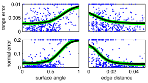
Figure 5: Our noise models predict range and normal errors (standard deviations) as functions of surface angle and edge distance (both with respect to the viewpoint).

IV Learning Discriminative Feature Models for Detection

Similarly to other recent object detection systems, our system computes a set of feature model placement score functions, in order to evaluate how well a given model placement hypothesis fits the scene according to different features, such as depth measurements, surface normals, edge locations, etc. In our early experiments with object detection using the generative object models in the previous section, the system was prone to make mis-classification errors, because some objects scored consistently higher on certain feature scores (presumably due to training set bias). Because of this problem, we trained discriminative, logistic regression models on each of the score components using the turntable scans with true model placements as positive training examples and a combination of correct object / wrong pose and wrong object / aligned pose as negative examples. Alignments of wrong objects were found by running the full object detection system (from the next section) with the wrong object on the turntable scans. By adding an (independent) discriminative layer to each of the feature score types, we were able to boost the classification accuracy of our system considerably.

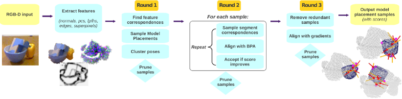
Figure 6: Single object detection pipeline.

V Detecting Single Objects in Clutter

The first stages of our object detection pipeline are very similar to many other state-of-the-art systems for 3-D object detection, with the exception that we rely more heavily on edge information. We are given as input an RGB-D image, such as from a Kinect. If environmental information is available, the image may be pre-processed by another routine to crop the image to an area of interest, and to label background pixels (e.g., belonging to a supporting surface).

As illustrated in figure 6, our algorithm starts by estimating a dense set of surface normals on the 3-D point cloud derived from the RGB-D image. From these surface normals, it estimates principal curvatures and FPFH features. In addition, it finds and labels three types of edges: range edges, image edges, and curvature edges—points in the RGB-D image where there is a depth discontinuity, an image intensity discontinuity, or high negative curvature. This edge information is converted into an edge image, which is formed from a spatially-blurred, weighted average of the three edge pixel masks. Intuitively, this edge image is intended to capture the relative likelihood that each point in the image is part of an object boundary. Then, the algorithm uses k-means to over-segment the point cloud based on positions, normals, and spatially-blurred colors (in CIELAB space) into a set of 3-D super-pixels.

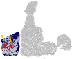
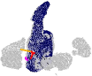
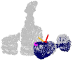
Figure 7: Examples of objects correctly aligned by BPA with only two correspondences.

Next, the algorithm samples possible oriented feature correspondences from the scene to the model. Then, for each correspondence, a candidate object pose is sampled using BPA. Given a set of sampled model poses from single correspondences, we then reject samples for which more than $20\%$ of a subset of $500$ randomly-selected model points project into free space—places where the difference between observed range image depth and predicted model depth is above $5cm$. Next, we run a pose clustering stage, where we group correspondences together whose sampled object poses are within $2.5cm$ and $\pi/16$ radians of one another. After pose clustering, we reject any sample with less than two correspondences, then re-sample object poses with BPA.

At this stage, we have a set of possible model placement hypotheses, with at least two features correspondences each. Because BPA uses additional orientation information, two correspondences is often all it takes to lock down a very precise estimate of an object’s pose when the correspondences are correct (Figure 7).

We proceed with a second round of model placement validation and rejection, this time using a scoring function that includes (1) range and normal differences, which are computed by projecting a new subset of $500$ randomly-selected model points into the observed range image, (2) visibility—the ratio of model points in the subset that are unoccluded, (3) edge likelihoods, computed by projecting the model’s edge points from the closest stored viewpoint into the observed edge image, and (4) edge visibility—the ratio of edge points that are unoccluded. Each of the feature score components is computed as a truncated (so as not to over-penalize outliers), average log-likelihood of observed features given model feature distributions. For score components (1) and (3), we weight the average log-likelihood by visibility probabilities, which are equal to 1 if predicted depth $<$ observed depth, and $N(\Delta\textrm{depth};0,\sigma_{vis})/N(0;0,1)$ otherwise.

After rejecting low-scoring samples in round 2, we then refine alignments by repeating the following three steps:

1. Assign observed super-pixel segments to the model.

2. Align model to the segments with BPA.

3. Accept the new alignment if the round 2 model placement score has improved.

In step (1), we sample a set of assigned segments according to the probability that each segment belongs to the model, which we compute as the ratio of segment points (sampled uniformly from the segment) that are within $1cm$ in position and $\pi/16$ radians in normal orientation from the closest model point. In step (2), we randomly extract a subset of 10 segment points from the set of assigned segments, find nearest neighbor correspondences from the keypoints to the model using the model distance transform, and then use BPA to align the model to the 10 segment points. Segment points are of two types—surface points and edge points. We only assign segment edge points to model edge points (as predicted from the given viewpoint), and surface points to surface points. Figures 1 and 8 show examples of object alignments found after segment alignment, where red points (with red normal vectors and orange principal curvature vectors sticking out of them) indicate surface point correspondences, and magenta points (with no orientations) are the edge point correspondences.

After round 2 alignments, the system removes redundant samples (with the same or similar poses), and then rejects low scoring samples using the scores found at the end of the segment alignment process. Then, it performs a final, gradient-based alignment, which optimizes the model poses with a local hill-climbing search to directly maximize model placement scores. Since this alignment step is by far the slowest, it is critical that the system has performed as much alignment with BPA and has rejected as many low-scoring samples as possible, to reduce the computational burden.

Finally, the system performs a third round of model placement evaluation, then sorts the pose samples by score and returns them. This third round of scoring includes several additional feature score components:

• Random walk score—starting from an observed point corresponding to the model, take a random walk in the edge image (to stay within predicted object boundaries), then measure the distance from the new observed point to the closest model point.

• Occlusion edge score—evaluate how well model occlusion edges (where the model surface changes from visible to occluded) fits the observed edge image.

• FPFH score—computes how well observed and model FPFH features match.

• Segment score—computes distances from segment points to nearest model points.

• Segment affinity score—measures how consistent the set of assigned segments is with respect to predicted object boundaries (as measured by the observed edge image, and by differences in segment positions and normals).

VI Detecting Multiple Objects in Clutter

To detect multiple objects in a scene, we run the individual object detector from the previous section to obtain the 50 best model placements for each model, along with their individual scores. Then, following Aldoma et. al [1], we use simulated annealing to optimize the subset of model placements (out of $50\times N$ for $N$ models) according to a multi-object-placement score, which we compute as a weighted sum of the following score components: (1) the average of single object scores, weighted by the number of observed points each object explains, (2) the ratio of explained / total observed points, and (3) a small penalty for the total number of detected objects. We also keep track of the top $100$ multi-object-placement samples found during optimization, so we can return a set of possible scene interpretations to the user (in the spirit of interpretation tree methods [7]). This is particularly useful for robot vision systems because they can use tracking, prior knowledge, or other sensory input (like touch) to provide additional validation of model placements, and we don’t want detections from a single RGB-D image to filter out possible model placements prematurely.

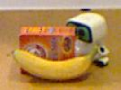
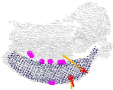
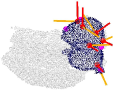
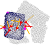
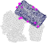
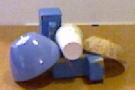
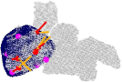
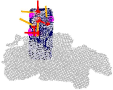
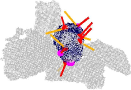
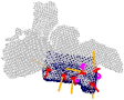
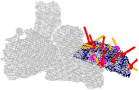
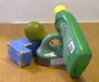
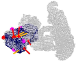
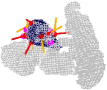
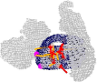
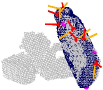
Figure 8: Object detections found with our system, along with the feature correspondences that BPA used to align the model. Surface features are indicated by red points, with lines sticking out of them to indicate orientations (red for normals, orange for principal curvatures). Edge features (which are orientation-less) are shown by magenta points.

Figure 9: The Clutter testing data set.

VII Experimental Results

We tested our object detection system on two Kinect-based data sets—the Kinect data set from Aldoma et. al [1] containing 35 models and 50 scenes, and a new, more difficult data set with many more occlusions and object pose variations that we collected for this paper which we will refer to as Clutter, which contains 18 models and 30 scenes (Figure 9). We used the same parameters (score component weights, number of samples, etc.) on both data sets. In table I, we compare the precision and recall of the top scene interpretations (multi-object-placement samples) of our method against Aldoma et. al on both data sets.

	this paper (BPA)		this paper (ICP)		Aldoma et. al [1]
	precision	recall	precision	recall	precision	recall
Kinect	89.4	86.4	71.8	71.0	90.9	79.5
Clutter	83.8	73.3	73.8	63.3	82.9	64.2

TABLE I: A comparison of precision and recall.

# samples	1	2	3	5	10	20
recall	73.3	77.5	80.0	80.8	83.3	84.2

TABLE II: Recall on the Clutter data set as a function of the number of scene interpretation samples.

Our algorithm (with BPA) achieves state-of-the art recall performance on both data sets. When multiple scene interpretations are considered, we achieve even higher recall rates (Table II). Our precisions are similar to the baseline method (slightly higher on Clutter, slightly lower on Kinect). We were unable to train discriminative feature models on the Kinect data set, because the original training scans were not provided. Training on scenes that are more similar to the cluttered test scenes is also likely to improve precision on the Clutter data set, since each training scan contained only one, fully-visible object.

VII-A BPA vs. ICP

We evaluated the benefits of our new alignment method, BPA, in two ways. First, we compared it to ICP by replacing the BPA alignment step in round 2 with an ICP alignment step. This resulted in a drop of $10\%$ in both precision and recall on the Clutter data.

For a second test of BPA, we initialized 50 model placements by adding random Gaussian noise to the ground truth poses for each object in each scene of the Clutter data set. Then, we ran BPA and ICP for 20 iterations on each of the model placements. We then computed the average of the minimum pose errors in each alignment trial, where the minimum at time $t$ in a given trial is computed as the minimum pose error from step $1$ to step $t$. (The justification for this measure is that this is approximately what the “accept if score improves” step of round 2 is doing.) As shown in figure 10, the pose errors decrease much faster in BPA.

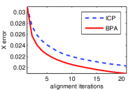
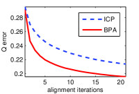
Figure 10: Comparing BPA with ICP. (Left) The average of the minimum position errors in each alignment trial. (Right) The average of the minimum orientation errors in each alignment trial.

VIII Related Work

Since the release of the Kinect in 2010, much progress has been made on 3-D object detection in cluttered RGB-D scenes. The two most succesful systems to date are Aldoma et. al [1] and Tang et. al [11]. Aldoma’s system is purely geometric, and uses SHOT features [12] for model-scene correspondences. It relies heavily on pose clustering of feature correspondences to suggest model placements. The main contribution of Aldoma’s system is that they jointly optimize multiple model placements for consistency, which inspired our own multiple object detection system.

Tang’s detection system uses both geometry and image features, and placed first in the ICRA 2011 Solutions in Perception instance recognition challenge. Their system relies heavily on being able to segment objects in the scene from one another, and most of the effort is spent on combining geometry and image features for classification of scene segments. It is unclear how well the system would perform if such segmentations are not easy to obtain, as is the case in our new Clutter data set.

The Bingham distribution was first used for 3-D cluttered object detection in Glover et. al [6]. However, that system was incomplete in that it lacked any alignment step, and differs greatly from this work because it did not use feature correspondences.

IX Conclusion and Future Work

We have presented a system for 3-D cluttered object detection which uses a new alignment method called Bingham Procrustean Alignment (BPA) to improve detections in highly cluttered scenes, along with a new RGB-D data set which contains much more clutter and pose variability than existing data sets. Our system relies heavily on geometry, and will clearly benefit from image and color models, such as in Tang et. al [11]. Our Clutter data set, while challenging, contains zero ambiguity, in that a human could easily detect all of the objects in their correct poses, given enough time to study the models. An important direction of future work is to handle ambiguous scenes, where the parts of objects that are visible are insufficient to perform unique alignments, and instead one ought to return distributions over possible model poses. In early experiments we have performed on this problem, the Bingham distribution has been a useful tool for representing orientation ambiguity.

APPENDIX

The Bingham Distribution. The Bingham distribution is commonly used to represent uncertainty on 3-D rotations (in unit quaternion form) [2, 5, 6]. For quaternions, its density function (PDF) is given by

$$p({\bf q};\Lambda,V)=\frac{1}{F}\exp\left\{\sum_{i=1}^{3}\lambda_{i}({\bf v_{i}}^{T}{\bf q})^{2}\right\}$$ (9)

where $F$ is a normalizing constant so that the distribution integrates to one over the surface of the unit hypersphere ${\mathbb{S}^{3}}$, the $\lambda$’s are non-positive ($\leq 0$) concentration parameters, and the ${\bf v_{i}}$’s are orthogonal direction vectors.

Product of Bingham PDFs. The product of two Bingham PDFs is given by adding their exponents:

$$\begin{split}f({\bf q};&\Lambda_{1},V_{1})f({\bf q};\Lambda_{2},V_{2})\\ &=\frac{1}{F_{1}F_{2}}\exp\left\{{\bf q}^{T}(\sum_{i=1}^{3}\lambda_{1i}{\bf v_{1i}}{\bf v_{1i}}^{T}+\lambda_{2i}{\bf v_{2i}}{\bf v_{2i}}^{T}){\bf q}\right\}\\ &=\frac{1}{F_{1}F_{2}}\exp\left\{{\bf q}^{T}(C_{1}+C_{2}){\bf q}\right\}\end{split}$$ (10)

After computing the sum $C=C_{1}+C_{2}$ in the exponent of equation 10, we compute the eigenvectors and eigenvalues of $C$, and then subtract off the lowest magnitude eigenvalue from each spectral component, so that only the eigenvectors corresponding to the largest $3$ eigenvalues (in magnitude) are kept, and $\lambda_{i}\leq 0\;\forall i$ (as in equation 9). We use the open-source Bingham Statistics Library to look up the normalization constant.

Estimating the Uncertainty on Feature Orientations. When we extract surface features from depth images, we estimate their 3-D orientations from their normals and principal curvature directions by computing the rotation matrix $R=\left[{\bf n}\;\;{\bf p}\;\;{\bf p^{\prime}}\right]$, where ${\bf n}$ is the normal vector, ${\bf p}$ is the principal curvature vector, and ${\bf p^{\prime}}$ is the cross product of ${\bf n}$ and ${\bf p}$. We take the quaternion associated with this rotation matrix to be the feature’s estimated orientation.

These orientation estimates may be incredibly noisy, not only due to typical sensing noise, but because on a flat surface patch the principal curvature direction is undefined and will be chosen completely at random. Therefore it is extremely useful to have an estimate of the uncertainty on each feature orientation that allows for the uncertainty on the normal direction to differ from the uncertainty on the principal curvature direction. Luckily, the Bingham distribution is well suited for this task.

To form such a Bingham distribution, we take the quaternion associated with $R$ to be the mode of the distribution, which is orthogonal to all the ${\bf v_{i}}$ vectors. Then, we set ${\bf v_{3}}$ to be the quaternion associated with $R^{\prime}=\left[{\bf n}\;\;-{\bf p}\;\;-{\bf p^{\prime}}\right]$, which has the same normal as the mode, but reversed principal curvature direction. In quaternion form, reversing the principal curvature is equivalent to the mapping:

$$(q_{1},q_{2},q_{3},q_{4})\;\;\rightarrow\;\;(-q_{2},q_{1},q_{4},-q_{3})\;\;.$$

We then take ${\bf v_{1}}$ and ${\bf v_{2}}$ to be unit vectors orthogonal to the mode and ${\bf v_{3}}$ (and each other). Given these ${\bf v_{i}}$’s, the concentration parameters $\lambda_{1}$ and $\lambda_{2}$ penalize deviations in the normal vector, while $\lambda_{3}$ penalizes deviations in the principal curvature direction. Therefore, we set $\lambda_{1}=\lambda_{2}=\kappa$ (we use $\kappa=-100$ in all our experiments in this paper), and we use the heuristic $\lambda_{3}=\max\{10(1-c_{1}/c_{2}),\kappa\}$, where $c_{1}/c_{2}$ is the ratio of the principal curvature eigenvalues. When the surface is completely flat, $c_{1}=c_{2}$ and $\lambda_{3}=0$, so the resulting Bingham distribution will be completely uniform in the principal curvature direction. When the surface is highly curved, $c_{1}\gg c_{2}$, so $\lambda_{3}$ will equal $\kappa$, and deviations in the principal curvature will be penalized just as much as deviations in the normal.

References

- [1] Aitor Aldoma, Federico Tombari, Luigi Di Stefano, and Markus Vincze. A global hypotheses verification method for 3d object recognition. In ECCV 2012, pages 511–524. Springer, 2012.
- [2] Matthew E Antone. Robust camera pose recovery using stochastic geometry. PhD thesis, Massachusetts Institute of Technology, Dept. of Electrical Engineering and Computer Science, 2001.
- [3] Dana H Ballard. Generalizing the hough transform to detect arbitrary shapes. Pattern recognition, 13(2):111–122, 1981.
- [4] P.J. Besl and N.D. McKay. A method for registration of 3-d shapes. IEEE Transactions on Pattern Analysis and Machine Intelligence, 14:239–256, 1992.
- [5] Christopher Bingham. An antipodally symmetric distribution on the sphere. The Annals of Statistics, 2(6):1201–1225, 1974.
- [6] Jared Glover, Radu Rusu, and Gary Bradski. Monte carlo pose estimation with quaternion kernels and the bingham distribution. In Proceedings of Robotics: Science and Systems, Los Angeles, CA, USA, June 2011.
- [7] W Eric L Grimson and Tomas Lozano-Perez. Localizing overlapping parts by searching the interpretation tree. Pattern Analysis and Machine Intelligence, IEEE Transactions on, (4):469–482, 1987.
- [8] Berthold KP Horn. Closed-form solution of absolute orientation using unit quaternions. JOSA A, 4(4):629–642, 1987.
- [9] David G Lowe. Object recognition from local scale-invariant features. In Computer Vision, 1999. The Proceedings of the Seventh IEEE International Conference on, volume 2, pages 1150–1157. Ieee, 1999.
- [10] Radu Bogdan Rusu, Nico Blodow, and Michael Beetz. Fast Point Feature Histograms (FPFH) for 3D Registration. In Proceedings of the IEEE International Conference on Robotics and Automation (ICRA), Kobe, Japan, May 12-17 2009.
- [11] Jie Tang, Stephen Miller, Arjun Singh, and Pieter Abbeel. A textured object recognition pipeline for color and depth image data. In Robotics and Automation (ICRA), 2012 IEEE International Conference on, pages 3467–3474. IEEE, 2012.
- [12] Federico Tombari, Samuele Salti, and Luigi Di Stefano. Unique signatures of histograms for local surface description. Computer Vision–ECCV 2010, pages 356–369, 2010.