Symplectic Cohomology and Duality for the Wrapped Fukaya Category

Abstract.

Consider the wrapped Fukaya category $\mathcal{W}$ of a collection of exact Lagrangians in a Liouville manifold. Under a non-degeneracy condition implying the existence of enough Lagrangians, we show that natural geometric maps from the Hochschild homology of $\mathcal{W}$ to symplectic cohomology and from symplectic cohomology to the Hochschild cohomology of $\mathcal{W}$ are isomorphisms, in a manner compatible with ring and module structures. This is a consequence of a more general duality for the wrapped Fukaya category, which should be thought of as a non-compact version of a Calabi-Yau structure. The new ingredients are: (1) Fourier-Mukai theory for $\mathcal{W}$ via a wrapped version of holomorphic quilts, (2) new geometric operations, coming from discs with two negative punctures and arbitrary many positive punctures, (3) a generalization of the Cardy condition, and (4) the use of homotopy units and A-infinity shuffle products to relate non-degeneracy to a resolution of the diagonal.

1. Introduction

It is a conjecture of Kontsevich [Kontsevich:1995uq] (inspired by mirror symmetry) that the quantum cohomology ring of a compact symplectic manifold $M$ should be isomorphic to the Hochschild cohomology

(1.1) $$\mathrm{HH}^{*}(\mathcal{F}(M))$$

of the Fukaya category $\mathcal{F}(M)$. There are at least two strong motivations for understanding this conjecture. For one, such an isomorphism would allow one to algebraically recover quantum cohomology along with its ring structure from computations of the Fukaya category. In another direction, Hochschild cohomology measures deformations of a category, so the conjecture has implications for the deformation theory of Fukaya categories; see e.g. [Seidel:2002ys].

We address a non-compact version of Kontsevich’s conjecture, in the setting of exact (non-compact) symplectic manifolds. The relevant symplectic objects are Liouville manifolds, exact symplectic manifolds with a convexity condition at infinity. Examples include cotangent bundles, affine complex varieties, and more general Stein manifolds. In this setting, there is an enlargement of the Fukaya category known as the wrapped Fukaya category

(1.2) $$\mathcal{W}:=\mathcal{W}(M),$$

whose objects include properly embedded (potentially non-compact) Lagrangians, and whose morphism spaces include intersection points as well as Reeb chords between Lagrangians at infinity. The wrapped Fukaya category is expected to be the correct mirror category to coherent sheaves on non-proper varieties, see e.g. [Abouzaid:2010ly] [Abouzaid:2011fk]. Moreover, it is the open-string, or Lagrangian, counterpart to a relatively classical invariant of non-compact symplectic manifolds, symplectic cohomology

(1.3) $$SH^{*}(M),$$

first defined by Cieliebak, Floer, and Hofer [Floer:1994uq] [Cieliebak:1995fk].

There are also existing geometric maps from the Hochschild homology

(1.4) $$\mathrm{HH}_{*}(\mathcal{W})$$

to symplectic cohomology [Abouzaid:2010kx] and from symplectic cohomology to the Hochschild cohomology [Seidel:2002ys]

(1.5) $$\mathrm{HH}^{*}(\mathcal{W}).$$

Thus, one can posit that a version of Kontsevich’s conjecture holds in this setting.

In this paper, we prove a non-compact version of Kontsevich’s conjecture for a Liouville manifold $M$ of dimension $2n$, assuming a non-degeneracy condition for $M$ first introduced by Abouzaid [Abouzaid:2010kx]. The reason for the non-degeneracy assumption is essentially this: to have any hope that symplectic cohomology be recoverable from the wrapped Fukaya category, it is important that the target manifold contain “enough Lagrangians.”

Definition 1.1.

A finite collection of Lagrangians $\{L_{i}\}$ is said to be essential if the natural map from Hochschild homology of the wrapped Fukaya category generated by $\{L_{i}\}$ to symplectic cohomology hits the identity element. Call $M$ non-degenerate if it admits any essential collection of Lagrangians.

The non-degeneracy condition is explicitly known for cotangent bundles [Abouzaid:2010fk] and some punctured Riemann surfaces [AbAurUnpublished]. In general, we expect that work of Bourgeois, Ekholm, and Eliashberg [BEE1published], suitably translated into the setting of the wrapped Fukaya category, would imply that every Stein manifold is non-degenerate, with essential Lagrangians given by the ascending co-cores of a plurisubharmonic Morse function. In a related direction, if $M$ is the total space of a Lefschetz fibration, upcoming work of Abouzaid and Seidel [AbSeInProgress] should also imply that $M$ is non-degenerate, with essential Lagrangians given by the Lefschetz thimbles of the fibration.

Our main result can then be stated as follows:

Theorem 1.1.

If $M$ is non-degenerate, then the natural geometric maps

(1.6) $$\mathrm{HH}_{*-n}(\mathcal{W})\stackrel{{\scriptstyle[\mathcal{OC}]}}{{\longrightarrow}}SH^{*}(M)\stackrel{{\scriptstyle[\mathcal{CO}]}}{{\longrightarrow}}\mathrm{HH}^{*}(\mathcal{W})$$

are both isomorphisms, compatible with Hochschild ring and module structures.

One consequence of Theorem 1.1 is that if $M$ is non-degenerate, the Hochschild homology and cohomology of $\mathcal{W}$ are isomorphic, up to a shift. In fact, a key step in proving Theorem 1.1 is first constructing a direct geometric Poincaré duality isomorphism

(1.7) $$\mathrm{HH}_{*-n}(\mathcal{W},\mathcal{B})\stackrel{{\scriptstyle\sim}}{{\longrightarrow}}\mathrm{HH}^{*}(\mathcal{W},\mathcal{B}),$$

for an arbitrary coefficient bimodule $\mathcal{B}$, which does not pass through $\mathrm{SH}^{*}(M)$. Such dualities have appeared before in the context of the algebraic geometry of smooth varieties. Van den Bergh [bergh:1998uq] [bergh:2002fk] was the first to observe a duality between Hochschild homology and cohomology for the coordinate ring of a smooth Calabi-Yau affine variety; see also [Krahmer:2007kx]. The relevant notion for us is a categorical, or non-commutative, version of smooth and Calabi-Yau, generalizing perfect complexes on a smooth Calabi-Yau variety. As in the algebro-geometric setting, smoothness is the prerequisite property that must be defined first.

Definition 1.2 (Kontsevich-Soibelman [Kontsevich:2006fk]).

An $A_{\infty}$ category $\mathcal{C}$ is (homologically) smooth if its diagonal bimodule is perfect, i.e., lies in the category split generated by tensor products of left and right Yoneda modules.

As a key technical ingredient in Theorem 1.1, we relate smoothness to the non-degeneracy condition.

Theorem 1.2.

If $M$ is non-degenerate, then $\mathcal{W}$ is smooth.

Definition 1.3.

An $A_{\infty}$ category $\mathcal{C}$ is a non-compact Calabi-Yau category if it is smooth and there is a Poincaré duality-type natural transformation

(1.8) $$\mathrm{HH}_{*-n}(\mathcal{C},\mathcal{B})\stackrel{{\scriptstyle\sim}}{{\longrightarrow}}\mathrm{HH}^{*}(\mathcal{C},\mathcal{B})$$

of functors from bimodules to chain complexes, inducing isomorphisms on homology. Such a natural transformation should be induced by an equivalence of bimodules

(1.9) $$\mathcal{C}\stackrel{{\scriptstyle\sim}}{{\longrightarrow}}\mathcal{C}^{!}[n].$$

Here, $\mathcal{C}^{!}$ is a perfect bimodule which represents, via tensoring, Hochschild cohomology.

(1.10) $$H^{*}(\mathcal{C}^{!}\otimes_{\mathcal{C}\!-\!\mathcal{C}}\mathcal{B})\cong\mathrm{HH}^{*}(\mathcal{C},\mathcal{B})$$

The bimodule $\mathcal{C}^{!}$, defined in Section 2.13, is known as the inverse dualizing bimodule. The non-compact Calabi-Yau terminology was introduced by Kontsevich and Soibelman [Kontsevich:2006fk] as a categorical abstraction of perfect complexes on a smooth, not necessarily proper Calabi-Yau variety.

With these definitions in place, we can state our second main result.

Theorem 1.3 (Duality for the wrapped Fukaya category).

Suppose $M$ is non-degenerate. Then, $\mathcal{W}$ is smooth and there is a geometric map

(1.11) $$\mathcal{CY}:\mathcal{W}\stackrel{{\scriptstyle\sim}}{{\longrightarrow}}\mathcal{W}^{!}[n]$$

giving $\mathcal{W}$ the structure of a non-compact Calabi-Yau category.

The geometric map (1.11) will be constructed from a new family of operations on the wrapped Fukaya category, parametrized by discs with multiple inputs and two (non-adjacent) outputs. The first-order term, for example, is a map

(1.12) $$\hom_{\mathcal{W}}(A,B)\rightarrow\hom_{Vect}(\hom_{\mathcal{W}}(C,D),\hom_{\mathcal{W}}(A,D)\otimes\hom_{\mathcal{W}}(C,B))$$

induced by a single disc with four boundary marked points, alternating as inputs and outputs, with a fixed cross ratio. A simplified version of these operations, in which the two outputs are adjacent, is used in a crucial way in [Abouzaid:2010kx].

Remark 1.1.

In contrast to the compact setting, symplectic cohomology and morphisms in the wrapped Fukaya category lack non-degenerate pairings, meaning one cannot trade inputs for outputs in Floer theoretic operations. From the perspective of topological field theory, the surfaces giving rise to operations on $\mathcal{W}$ must have at least one output. Thus, the two-output operations considered here and in [Abouzaid:2010kx] give new operations on $\mathcal{W}$.

In order to deduce Theorem 1.1 from Theorem 1.3, we invoke a holomorphic-curve version of the Cardy condition from topological field theory:

Theorem 1.4 (Generalized Cardy Condition).

There is a (homotopy)-commutative diagram

(1.13)

Here $[\mathcal{CY}_{\#}]$ is the map induced from (1.11) on the level of Hochschild homology, and $\bar{\mu}$ is a map induced by compositions of $A_{\infty}$ multiplication.

The proof follows from analyzing the degenerations of operations parametrized by families of annuli with marked points on both boundary components.

The map $[\bar{\mu}]$, a special case of the map appearing in the identification

$$H^{*}(\mathcal{W}^{!}\otimes_{\mathcal{W}\!-\!\mathcal{W}}\mathcal{B})\simeq\mathrm{HH}^{*}(\mathcal{W},\mathcal{B}),$$

is an isomorphism whenever $\mathcal{W}$ is smooth. So (1.13) provides a commutative diagram in which the top and right maps are isomorphisms. Theorem 1.3, which concerns the bottom and left maps, then follows from the observation that

Proposition 1.1.

If $M$ is non-degenerate, then $[\mathcal{OC}]$ is surjective and $[\mathcal{CO}]$ is injective.

Proposition 1.1 is a simple consequence of the compatibility of $[\mathcal{OC}]$ and $[\mathcal{CO}]$ with algebraic structures: $[\mathcal{CO}]$ is a morphism of rings, and $[\mathcal{OC}]$ is a morphism of $SH^{*}(M)$ modules, using the map $[\mathcal{CO}]$ and the module structure of Hochschild homology over cohomology. As an alternative to Proposition 1.1, our proof of Theorem 1.3 also directly establishes that $[\mathcal{CO}]$ is an isomorphism, which suffices.

As one application of this work, whenever $M$ is non-degenerate, we find two methods for explicitly recovering the ring structure on $SH^{*}(M)$ from the wrapped Floer theory of any essential collection of Lagrangians: one directly from Hochschild cohomology using its product, and one from Hochschild homology using $A_{\infty}$ structure maps and the new geometric operations $\mathcal{CY}$. In the case $M$ is Stein, formulae formally similar to the latter description have appeared in [BEE2], phrased in terms of the symplectic field theory invariants of attaching Legendrians of a suitable handle decomposition. Taking our formulae applied to the (conjecturally essential) collection of ascending Lagrangian co-cores for the same decomposition, it is natural to expect that the underlying algebraic structures should be related.

Remark 1.2.

Going further than the product, one might hope to recover all field-theoretic operations on symplectic cohomology from the Hochschild homology of the wrapped Fukaya category, at least in the sense of [Costello:2006vn], [Lurie:2009fk], or [Kontsevich:uq]. We have not attempted to do so here, but have two remarks. First, the work of [Costello:2006vn] is not immediately applicable, as it is formulated under different hypotheses—see instead [Lurie:2009fk]*Remark 4.2.17 for a version relevant to the wrapped Fukaya category. Second, in order to cite a theorem from topological field theory, there is an additional criterion to check: the Hochschild cycle whose image is $1\in SH^{*}(M)$ should be a homotopy fixed point the $S^{1}$ action on the Hochschild complex (the one inducing the Connes’ $B$ operator). We leave this for future work.

Theorem 1.3 will follow from the construction and analysis of a natural functor $\mathbf{M}$, coming from operations parametrized by quilted strips, from the wrapped Fukaya category of the product $M^{-}\times M$ to bimodules over $\mathcal{W}$. Quilted strips have been used in the compact setting [Wehrheim:2010fk] [Wehrheim:2010uq] to associate a functor between the (cohomology-level) Fukaya categories of $M$ and $N$ to a (monotone) Lagrangian correspondence $L\subset M^{-}\times N$ (an extension to the chain level is forthcoming [MWW1]). Using a variant of the original parameter spaces appearing in [Mau:2010lq], we give a direct chain-level construction of a version of this functor for the wrapped Fukaya category. The fullness of this functor, which contains both open-closed operations and morphisms with two output punctures in its definition, will have implications for the isomorphism (1.11). The need for such a construction partially explains the length of this paper. The idea that moduli spaces of quilts involving the diagonal $\Delta$ should be related to open-closed string maps is not new—see e.g., [Abouzaid:2010vn]. However, to our knowledge, our exploitation of the relationship between $\mathbf{M}$ and the morphism $\mathcal{CY}$ is new.

In more detail, we define an $A_{\infty}$ category

$$\mathcal{W}^{2}$$

associated to the product $M^{-}\times M$, with two types of objects: products $L_{i}\times L_{j}$ of objects in $\mathcal{W}$, and the diagonal $\Delta$. For purely technical reasons, we do not call this the wrapped Fukaya category of the product, as compositions in this category are defined using split Hamiltonians, which are not in the usual class of admissible Hamiltonians on the Liouville manifold $M^{-}\times M$, see e.g., [Oancea:2006oq]. However, this category has the property (reflecting an observation initially due to Floer [Floer:1988kx]) that

(1.14) $$H^{*}(\hom_{\mathcal{W}^{2}}(\Delta,\Delta))=SH^{*}(M).$$

Then, we construct an $A_{\infty}$ functor

(1.15) $$\mathbf{M}:\mathcal{W}^{2}\longrightarrow\mathcal{W}\mathrm{\!-\!mod\!-\!}\mathcal{W}$$

from $\mathcal{W}^{2}$ to the category of bimodules over $\mathcal{W}$, satisfying the following properties: on the level of objects, a product Lagrangian $K\times L$ is sent to the corresponding tensor product of left and right Yoneda modules $\mathcal{Y}^{l}_{K}\otimes\mathcal{Y}^{r}_{L}$, and the diagonal $\Delta$ is sent to the diagonal bimodule $\mathcal{W}_{\Delta}$. Moreover, on morphism complexes,

(1.16) $$H^{*}(\mathbf{M}^{1}):H^{*}(\hom_{\mathcal{W}^{2}}(\Delta,\Delta))\longrightarrow H^{*}(\hom_{\mathcal{W}\mathrm{\!-\!mod\!-\!}\mathcal{W}}(\mathcal{W}_{\Delta},\mathcal{W}_{\Delta}))$$

agrees with the map $[\mathcal{CO}]$ between symplectic cohomology and Hochschild homology. Similarly, we show the first order part of the map (1.11) appears in the functor $\mathbf{M}$ applied to the morphism complex $\hom_{\mathcal{W}^{2}}(\Delta,K\times L)$. The functor $\mathbf{M}$ we construct has the feature (unlike versions that use a more general class of Lagrangian correspondences and varying width strips) that no really new analysis is used in its construction beyond that which appears in the construction of open-closed operations and (1.11). Also, by using bimodules as a target instead of functors, we avoid passing to a wrapped version of the extended Fukaya category [Wehrheim:2010fk] whose objects consist of sequences of Lagrangian correspondences (this was suggested to us by Ma’u [Mau:2010lq]). Thus, it can be thought of as a lightweight construction of the quilt functor.

We establish the following crucial fact about the functor $\mathbf{M}$, which follows from a variant of the Yoneda lemma for bimodules:

Proposition 1.2.

$\mathbf{M}$ is full on the full sub-category of $\mathcal{W}^{2}$ consisting of product Lagrangians.

Thus, Theorem 1.2, the quasi-isomorphism in Theorem 1.3 (and indeed, more directly the statement that $\mathcal{CO}$ is an isomorphism) are consequences of the following:

Theorem 1.5 (Resolution of the diagonal).

Suppose $M$ is non-degenerate, with essential collection $\mathcal{L}$. Then in the category $\mathcal{W}^{2}$, $\Delta$ is split-generated by products of objects in the collection $\mathcal{L}$. By Proposition 1.2, $\mathbf{M}$ is full on $\mathcal{W}^{2}$.

Theorem 1.5, the most technical of our results, involves checking a split-generation criterion introduced into the symplectic literature by Abouzaid [Abouzaid:2010kx]: In $\mathcal{W}^{2}$, $\Delta$ is split-generated by the subcategory $\mathcal{W}^{2}_{split}$ consisting of product Lagrangians if and only if the cohomology-level unit $1\in H^{*}(\hom_{\mathcal{W}^{2}}(\Delta,\Delta))$ is in the image of a natural map from a certain bar complex involving $\Delta$ and $\mathcal{W}^{2}_{split}$:

(1.17) $$[\mu]:H^{*}(\mathcal{Y}^{r}_{\Delta}\otimes_{\mathcal{W}^{2}_{split}}\mathcal{Y}^{l}_{\Delta})\longrightarrow H^{*}(\hom_{\mathcal{W}^{2}}(\Delta,\Delta)).$$

As part of the proof of Theorem 1.5, we give a natural chain-level comparison map

(1.18) $$[\Gamma]:\rm{HH}_{*}(\mathcal{W},\mathcal{W})\longrightarrow H^{*}(\mathcal{Y}^{r}_{\Delta}\otimes_{\mathcal{W}^{2}_{split}}\mathcal{Y}^{l}_{\Delta})$$

between the Hochschild homology and the bar complex in (1.17). We also prove that it intertwines the non-degeneracy condition and the split-generation condition, so there is a commutative diagram

(1.19)

which translates the non-degeneracy condition into (1.17). This comparison map from morphisms and $A_{\infty}$ structure maps in $\mathcal{W}$ to those in $\mathcal{W}^{2}$ involves an $A_{\infty}$ generalization of the Eilenberg-Zilberg shuffle product map from algebraic topology (see e.g., [Loday:1992fk]*§4.2), which involves summing over all possible ways to insert units. In order for such a map to be a chain map in the $A_{\infty}$ setting, we are led to geometrically strictify units in both $\mathcal{W}$ and $\mathcal{W}^{2}$, using an implementation of the homotopy units of [Fukaya:2009ve] [Fukaya:2009qf]. This construction, which may be of independent interest, is the second reason for the length of this paper.

1.1. Contents of paper

In Section 2, we collect necessary facts about $A_{\infty}$ categories, modules and bimodules. These include definitions of these objects, constructions of differential graded categories associated to modules and bimodules, and a discussion of various tensor products associated to modules and bimodules. We recall definitions of the Hochschild co-chain and chain complexes, along with the ring and module structures on these complexes. In fact, we give two different chain-level models for each complex, one that seems more common in the symplectic literature, and a quasi-isomorphic one coming from categories of bimodules. We discuss canonical modules and bimodules coming from the Yoneda embedding, and the notion of homological smoothness. We discuss the notion of split-generation by a subcategory and recall a criterion for split-generation. Finally, we introduce operations of duality for modules and bimodules, in order to define a dual bimodule

(1.20) $$\mathcal{B}^{!}$$

associated to any bimodule $\mathcal{B}$. Specializing to the diagonal bimodule $\mathcal{C}_{\Delta}$ over an $A_{\infty}$ category $\mathcal{C}$, we obtain the so-called inverse dualizing bimodule

(1.21) $$\mathcal{C}^{!}:=(\mathcal{C}_{\Delta})^{!}.$$

We prove that, assuming $\mathcal{C}$ is smooth, tensoring a bimodule with $\mathcal{C}^{!}$ amounts to taking the Hochschild cohomology of the bimodule, via a natural comparison map

(1.22) $$[\mu_{\mathcal{B}}]:H^{*}(\mathcal{C}^{!}\otimes_{\mathcal{C}\!-\!\mathcal{C}}\mathcal{B})\stackrel{{\scriptstyle\sim}}{{\longrightarrow}}\mathrm{HH}^{*}(\mathcal{C},\mathcal{B}),$$

an $A_{\infty}$-categorical generalization of a result due to Van den Bergh [bergh:1998uq] [bergh:2002fk].

In Sections 3, 4, 5, and 6 we construct and prove various facts about the main geometric players in Theorem 1.1. First, in Section 3, we present our geometric setup, recalling the notions of Liouville manifolds, symplectic cohomology, and wrapped Floer cohomology. In Section 4, we introduce the moduli space of genus 0 open-closed strings, which are genus 0 bordered surfaces with signed boundary and interior marked points equipped with an additional framing around each interior point, restricting to at most one interior output or two boundary outputs. We define Floer data for such moduli spaces, and construct Floer-theoretic operations for submanifolds of these moduli spaces. In Section 5, we consider operations induced by various families of submanifolds. For spheres with two inputs, we obtain the product on symplectic cohomology and from discs with arbitrarily many inputs and one output, we construct $A_{\infty}$ structure maps for the wrapped Fukaya category. Then, using families of discs with boundary and interior marked points, we define the open-closed maps

(1.23) $$[\mathcal{OC}]:\mathrm{HH}_{*-n}(\mathcal{W},\mathcal{W})\longrightarrow SH^{*}(M)$$

from Hochschild homology to symplectic cohomology and

(1.24) $$[\mathcal{CO}]:SH^{*}(M)\longrightarrow\mathrm{HH}^{*}(\mathcal{W},\mathcal{W})$$

from symplectic cohomology to Hochschild cohomology. Actually we define two chain-level versions each of these open-closed maps, one for each of our two explicit Hochschild chain and co-chain complexes from Section 2, and prove that they are homotopic. Finally, we prove some basic facts about the open-closed maps: the map $[\mathcal{CO}]$ is a morphism of rings, giving $\mathrm{HH}_{*-n}(\mathcal{W},\mathcal{W})$ the structure of a module over $SH^{*}(M)$ via the existing module structure of $\mathrm{HH}_{*}(\mathcal{W},\mathcal{W})$ over $\mathrm{HH}^{*}(\mathcal{W},\mathcal{W})$. With respect to this induced module structure, we show that the map $[\mathcal{OC}]$ is a morphism of $SH^{*}(M)$ modules. This immediately implies Proposition 1.1. Also, in Section 6, we recall operations arising from unstable surfaces, the identity morphism and homology unit.

In Section 7, a core technical section, we introduce Floer-theoretic operations parametrized by new abstract moduli spaces of pairs of partially glued discs modulo simultaneous automorphisms. We begin with the moduli space of pairs of discs, a moduli space that not identical to the product of the moduli space of discs with itself, which arises as a further quotient by relative automorphisms of factors. We construct a compactification of these spaces, along the way examining natural subspaces where various boundary points are identified. We define a partial gluing operation, on loci where various boundary components between factors coincide, from pairs of discs to genus 0 open-closed strings. Finally, we define Floer data and operations for families of such partially glued pairs of discs. This construction allows us in subsequent sections to rapidly construct models for Floer theory on the product and the quilt functor, using operations entirely in $M$.

In Section 8, we move to the product manifold

(1.25) $$M^{-}\times M,$$

a symplectic manifold which contains two natural classes of Lagrangians, split Lagrangians of the form $L_{i}\times L_{j}$ and the diagonal $\Delta$. In general, there are technical issues defining wrapped Floer theory and symplectic cohomology of products, coming from a technical point that in order to define Floer theoretic invariants for $M$, we have fixed a choice of contact boundary at infinity, and such a choice does not determine a choice of contact boundary at infinity for the product (rather, it defines a “normal-crossings contact manifold”). See for example [Oancea:2006oq] for a solution in the case of symplectic cohomology. Instead of solving these issues, in Section 8 we use split Hamiltonians to reduce the moduli spaces of discs in $M^{-}\times M$ (for Lagrangians in $\mathrm{ob\ }\mathcal{W}^{2}$) to glued pairs of discs in $M$, producing a model

(1.26) $$\mathcal{W}^{2}$$

for the wrapped Fukaya category of $M^{-}\times M$. The reason we needed glued pairs of discs and not disjoint pairs of discs comes of course from the presence of the diagonal, beginning with a classical observation that the self-Lagrangian Floer cohomology of the diagonal $\Delta\subset M^{-}\times M$ computes the ordinary Floer cohomology of $M$.

In Section 9, we study spaces of quilted strips, first introduced by Ma’u [Mau:2010lq] as a variant of the quilted surfaces of Wehrheim-Woodward and Ma’u-Wehrheim-Woodward [Wehrheim:2010fk] [Mau:2010fk]. Using an embedding from labeled quilted strips with seam labels in $\mathrm{ob\ }\mathcal{W}^{2}$ into glued pairs of discs, we obtain Floer-theoretic operations, which we show in Proposition 9.3 give an $A_{\infty}$ functor

(1.27) $$\mathbf{M}:\mathcal{W}^{2}\longrightarrow\mathcal{W}\mathrm{\!-\!mod\!-\!}\mathcal{W}$$

where $\mathcal{W}\mathrm{\!-\!mod\!-\!}\mathcal{W}$ is the category of bimodules over $\mathcal{W}$. This is a bimodule version of a functoriality result in the sense of [Wehrheim:2010fk] for the wrapped Fukaya category (this version formulated by [Mau:2010lq]). The relation to open-closed operations is this: we see that the diagonal $\Delta$ is sent to the diagonal bimodule $\mathcal{W}_{\Delta}$, and the first order term

(1.28) $$[\mathbf{M}^{1}]:SH^{*}(M)=HW^{*}(\Delta,\Delta)\longrightarrow\hom_{\mathcal{W}\mathrm{\!-\!mod\!-\!}\mathcal{W}}(\mathcal{W}_{\Delta},\mathcal{W}_{\Delta})\simeq\mathrm{HH}^{*}(\mathcal{W},\mathcal{W})$$

is exactly the closed-open map $[\mathcal{CO}]$ (Proposition 9.7—in fact, it agrees on the chain level with the second chain-level closed-open map we defined). We verify that $\mathbf{M}$ sends split Lagrangians to tensor products of Yoneda modules, and hence, by a version of the Yoneda lemma for bimodules, $\mathbf{M}$ is always full on split Lagrangians (Proposition 1.2). A related observation was first made by Abouzaid-Smith [Abouzaid:2010vn], in the compact setting for an analogous functor with target category endofunctors of extended Fukaya categories (instead of bimodules).

In Section 10, another technical section, we introduce the tool of homotopy units, first constructed geometrically by Fukaya, Oh, Ohta, and Ono [Fukaya:2009qf] in the compact setting. Homotopy units allow one to geometrically strictify units in an $A_{\infty}$ category, which otherwise only exist on the homology level. A basic consequence of homotopy units is that one can talk about Floer-theoretic operations on the Fukaya category induced from families of surfaces by forgetting boundary marked points. Thus, we first explore and construct Floer theoretic operations with forgotten boundary points (Section 10.1). Then, we develop homotopies between such Floer theoretic operations and ones in which we had glued in geometric units instead of forgetting. In order to obtain a quasi-isomorphic category, we must, as in [Fukaya:2009qf], construct operations corresponding to all possible higher homotopies. When done for glued pairs of discs, (only allowing ourselves to forget boundary marked points with asymptotic to morphisms between product Lagrangians), we obtain a category quasi-isomorphic to $\mathcal{W}^{2}$. The resulting category, which we call

(1.29) $$\tilde{\mathcal{W}}^{2}$$

is identical to $\mathcal{W}^{2}$, except that its morphism spaces contain additional formal elements of the form $e^{+}\otimes x$, $x\otimes e^{+}$, which we term one-sided homotopy units, (there are also formal elements $f\otimes x$, $x\otimes f$, corresponding to the homotopy between the geometric unit and $e^{+}$). $A_{\infty}$ operations on $\tilde{\mathcal{W}}^{2}$ involving $e^{+}$ elements involve forgetful maps applied to boundary marked points, and operations involving $f$ elements correspond to homotopies between forgetful maps and geometric units. A crucial observation made in Proposition 10.11 asserts that $A_{\infty}$ operations on $\tilde{\mathcal{W}}^{2}$ reduce to operations on $\mathcal{W}$ when some of the inputs are one-sided homotopy units.

In Section 11, we use the tools developed in the previous section to prove that if $M$ is non-degenerate, then $\Delta$ is split-generated by product Lagrangians in $\mathcal{W}^{2}$ (the contents of Theorem 1.5). This, along with the existence of the functor $\mathbf{M}$ which is full on product Lagrangians (Proposition 1.2) implies $\mathbf{M}$ is full on $\Delta$, and in particular $\mathcal{W}$ is smooth (Theorem 1.2). As an immediate consequence, the map from $SH^{*}(M)\longrightarrow\mathrm{HH}^{*}(\mathcal{W},\mathcal{W})$, which we have shown is a part of the data of $[\mathbf{M}^{1}]$, is an isomorphism, proving part of Theorem 1.1. To prove split-generation of $\Delta$, we construct the map $\Gamma$ described in (1.18) between the Hochschild homology of of $\mathcal{W}$ and a bar complex appearing in an algebraic split-generation criterion for $\Delta$ in $\tilde{\mathcal{W}}^{2}$ (see (1.29)), discussed in Section 2. The map $\Gamma$, an $A_{\infty}$ version of the shuffle product, uses the formal elements $e^{+}\otimes x$ and $x\otimes e^{+}$ in an essential way, and is a chain map intertwining the natural maps in the non-degeneracy and split-generation criteria as in (1.19) thanks to identities involving operations in $\tilde{\mathcal{W}}^{2}$ applied to formal units, Proposition 10.11. As a consequence, we deduce that product Lagrangians split generate $\Delta$, whenever $M$ is non-degenerate.

Since $\mathcal{W}$ is smooth, by Section 2, the bimodule $\mathcal{W}^{!}$ is perfect and represents Hochschild cohomology. In Section 12, we construct a geometric morphism of bimodules

(1.30) $$\mathcal{CY}:\mathcal{W}_{\Delta}\longrightarrow\mathcal{W}^{!}[n],$$

coming from new operations controlled by discs with two negative punctures and arbitrary positive punctures. To first order, we show this map agrees on the chain level with the first order term of the quilt functor

$$\mathbf{M}^{1}:\hom_{\mathcal{W}^{2}}(\Delta,K\times L)\longrightarrow\hom_{\mathcal{W}\!-\!\mathcal{W}}(\mathcal{W}_{\Delta},\mathcal{Y}^{l}_{K}\otimes\mathcal{Y}^{r}_{K})$$

constructed in Section 9 (Proposition 12.2). This identification, which implies Theorem 1.3, relies on the identities for $\mathcal{W}^{2}$:

(1.31) $$\hom_{\mathcal{W}^{2}}(\Delta,K\times L) \simeq\hom_{\mathcal{W}}(K,L)[-n],$$

(1.32) $$\hom_{\mathcal{W}^{2}}(K\times L,\Delta) \simeq\hom_{\mathcal{W}}(L,K),$$

(see Propositions 8.2 and 8.1). The latter identity has a categorical shadow (Proposition 2.11), but the former is very special to categories expected to be non-compact Calabi-Yau. For example, we do not expect Fukaya-Seidel categories of products of Lefschetz fibrations to satisfy (1.31).

In Section 13, we analyze operations coming from spaces of annuli with many positive boundary marked points on both boundaries and one negative boundary marked point on the outer boundary. We show that degenerations of a codimension 1 family of these annuli give a relation between $\mathcal{CY}$ and standard open-closed maps, proving Theorem 1.4. In the relevant diagram (1.13), we have shown in Section 2 that if $\mathcal{W}$ is smooth, then the vertical map $\bar{\mu}$ is always a quasi-isomorphism. We have also shown in Sections 12 and 11 that $[\mathcal{CO}]$ and $[\mathcal{CY}_{\#}]$ are isomorphisms. This implies that $[\mathcal{OC}]$ is also a quasi-isomorphism, completing the proof of Theorem 1.1.

Finally, in Section 14, we explore a few basic consequences of this work. For one, we establish in Section 14.1 a converse result that if $\Delta$ is split-generated by product Lagrangians, then $M$ is non-degenerate, so Theorem 1.1 continues to apply. Then, furthering the relation between Theorem 1.3 and Poincaré duality, we demonstrate in Section 14.2 that the unique pre-image $\sigma\in\mathrm{HH}_{*}(\mathcal{W},\mathcal{W})$ of $1\in SH^{*}(M)$, which we call a fundamental class, satisfies

(1.33) $$\cdot\cap\sigma:\mathrm{HH}^{*}(\mathcal{W},\mathcal{W})\stackrel{{\scriptstyle\sim}}{{\longrightarrow}}\mathrm{HH}_{*-n}(\mathcal{W},\mathcal{W}).$$

As an application of this circle of ideas, in Section 14.3 we give an explicit formula for the $SH^{*}(M)$ pair of pants product on Hochschild homology, using only the operations given by $\mathcal{CY}$ and the $A_{\infty}$ structure maps of $\mathcal{W}$.

In Appendix A, we prove a compactness result for for the moduli spaces controlling our Floer-theoretic operations, which may be of independent interest. Such a result is necessary as we are considering spaces of maps into a non-compact target $M$. In order to apply standard Gromov compactness results, one first must show that spaces of maps with fixed asymptotics are a priori bounded in the target. Such results for the wrapped Fukaya category have generally used a convexity argument [Abouzaid:2010ly] [Abouzaid:2010kx] or maximum principles [Seidel:2010fk], which rely in a strong way on the Hamiltonian flow used having a rigid form at infinity. However, to construct higher operations on symplectic cohomology, we have found it necessary to introduce small time and surface dependent perturbations that are not of this rigid form. Our solution fuses standard maximum principle and convexity arguments with a slight strengthening of the maximum principle for cylindrical regions of the source surface, dating back to work of Floer-Hofer [Floer:1994uq] and Cieliebak [Cieliebak:1994fk], and also used successfully by Oancea [Oancea:2008fk].

Lastly, in Appendix B, we discuss ingredients necessary to construct all of our operations with appropriate signs over ${\mathbb{Z}}$ (or alternatively a field of characteristic other than $2$). We begin the appendix with a discussion of orientation lines, recall relevant results that orient moduli spaces of maps, give orientations for the abstract moduli spaces we use, and demonstrate the theory with a complete calculation of signs in an example.

Conventions

We will for simplicity work over a field ${\mathbb{K}}$ of arbitrary characteristic (though our results seem valid more generally, e.g., over ${\mathbb{Z}}$). If $f$ denotes any chain map, we will use $[f]$ to denote the resulting homology-level map.

Acknowledgements

I would like to thank Mohammed Abouzaid and Denis Auroux (my Ph.D. advisor) for all of their help with this work and for suggesting this line of inquiry. As should be evident, the work here has been greatly influenced by the paper [Abouzaid:2010kx]. I am also grateful to Yakov Eliashberg and Paul Seidel for many enlightening discussions, Sikimeti Ma’u for explaining her work [Mau:2010lq] on quilted strips, and Jonathan Bloom for comments on an earlier draft. Lastly, I would like to thank the organizers and attendees of the 2009 AIM Conference on Cyclic Homology and Symplectic Topology for a stimulating atmosphere that directly inspired much of this work. This work was partly completed with the support of an NSF Graduate Fellowship.

2. Algebraic preliminaries

We give an overview of the algebraic technology appearing in this paper: $A_{\infty}$ categories, functors, modules, bimodules, and Hochschild homology and cohomology. We also recall some useful but slightly more involved algebraic details: the $A_{\infty}$ Yoneda embedding, the Künneth formula for split bimodules, pullbacks of modules and bimodules along functors, and ring/module structures on Hochschild groups. We also introduce notions of module and bimodule duality, in order to ultimately define a natural bimodule $\mathcal{C}^{!}$ associated to any $A_{\infty}$ category $\mathcal{C}$. None of the material is completely new, although some of it does not seem to have appeared in the $A_{\infty}$ or symplectic context.

2.1. $A_{\infty}$ algebras and categories

Definition 2.1.

An $A_{\infty}$ algebra $\mathcal{A}$ is a graded vector space $\mathcal{A}$ together with maps

(2.1) $$\mu^{s}_{\mathcal{A}}:\mathcal{A}^{\otimes s}\rightarrow\mathcal{A},\ s\geq 1$$

of degree $2-s$ such that the following quadratic relation holds, for each $k$:

(2.2) $$\sum_{i,l}(-1)^{\maltese_{i}}\mu^{k-l+1}_{\mathcal{A}}(x_{k},\ldots,x_{i+l+1},\mu^{l}_{\mathcal{A}}(x_{i+l},\ldots,x_{i+1}),x_{i},\ldots,x_{1})=0.$$

where the sign is determined by

(2.3) $$\maltese_{i}:=|x_{1}|+\cdots+|x_{i}|-i.$$

Remark 2.1.

The parity of $\maltese_{i}$ is the same as the sum of the reduced degrees $\sum_{j=1}^{i}||x_{j}||$. Here $||x_{j}||=|x_{j}|-1$ is the degree of $x_{j}$ thought of as an element of the shifted vector space $\mathcal{A}[1]$. Thus, $\maltese_{i}$ can be thought of as a Koszul-type sign arising as $\mu^{l}$ acts from the right.

The first few $A_{\infty}$ relations are, up to sign:

(2.4) $$\mu^{1}(\mu^{1}(x)) =0$$

(2.5) $$\mu^{1}(\mu^{2}(x_{0},x_{1})) =\pm\mu^{2}(\mu^{1}(x_{0}),x_{1})\pm\mu^{2}(x_{0},\mu^{1}(x_{1}))$$

$$\pm\mu^{2}(\mu^{2}(x_{0},x_{1}),x_{2})\mp\mu^{2}(x_{0},\mu^{2}(x_{1},x_{2})) =\mu^{1}(\mu^{3}(x_{0},x_{1},x_{2}))\pm\mu^{3}(\mu^{1}(x_{0}),x_{1},x_{2})$$

(2.6) $$\pm\mu^{3}(x_{0},\mu^{1}(x_{1}),x_{2})\pm\mu^{3}(x_{0},x_{1},\mu^{1}(x_{2}))$$

In particular, the first few equations above imply that $\mu^{1}$ is a differential, (up to a sign change) $\mu^{2}$ descends to a product on $H^{*}(\mathcal{A},\mu^{1})$, and the resulting homology-level product $H^{*}(\mu^{2})$ is associative. $\mu^{3}$ can be thought of as the associator, and the other $\mu^{k}$ are higher homotopies for associativity.

One can also recast the notion of an $A_{\infty}$ algebra in the following way: Let

(2.7) $$T\mathcal{A}[1]=\bigoplus_{i>0}\mathcal{A}[1]^{\otimes i}$$

be the tensor co-algebra of the shifted $\mathcal{A}[1]$.

Given any map $\phi:T\mathcal{A}[1]\rightarrow\mathcal{A}[1]$, there is a unique so-called hat extension

(2.8) $$\hat{\phi}:T\mathcal{A}[1]\rightarrow T\mathcal{A}[1]$$

specified as follows:

(2.9) $$\hat{\phi}(x_{k}\otimes\cdots\otimes x_{1}):=\sum_{i,j}(-1)^{\maltese_{i}}x_{k}\otimes\cdots\otimes x_{i+j+1}\otimes\phi^{j}(x_{i+j},\ldots,x_{i+1})\otimes x_{i}\otimes\cdots\otimes x_{1}.$$

The (shifted) $A_{\infty}$ operations $\mu^{i}$ fit together to form a map

(2.10) $$\mu:T\mathcal{A}[1]\rightarrow\mathcal{A}[1]$$

of total degree 1. Then the $A_{\infty}$ equations, which can be re-expressed as one equation

(2.11) $$\mu\circ\hat{\mu}=0,$$

are equivalent to the requirement that $\hat{\mu}$ is a differential on $T\mathcal{A}[1]$

(2.12) $$\hat{\mu}^{2}=0.$$

Remark 2.2.

Actually, the hat extension $\hat{\phi}$ defined above is the unique extension satisfying the graded co-Leibniz rule with respect to the natural co-product $\Delta:T\mathcal{A}[1]\longrightarrow T\mathcal{A}[1]\otimes T\mathcal{A}[1]$, given by

(2.13) $$\Delta(x_{n}\otimes\cdots\otimes x_{1})=\sum_{i}(x_{n}\otimes\cdots\otimes x_{i+1})\otimes(x_{i}\otimes\cdots\otimes x_{1}).$$

In this way, the association of $(T\mathcal{A},\hat{\mu})$ to the $A_{\infty}$ algebra $(\mathcal{A},\mu)$ gives an embedding of $A_{\infty}$ algebra structures on a vector space to differential-graded co-algebra structures on the tensor algebra over that vector space. The chain complex $(T\mathcal{A},\hat{\mu})$ is called the bar complex of $\mathcal{A}$.

The discussion so far generalizes in a straightforward manner to the categorical setting.

Definition 2.2.

An $A_{\infty}$ category $\mathcal{C}$ consists of the following data:

• a collection of objects $\mathrm{ob\ }\mathcal{C}$

• for each pair of objects $X,X^{\prime}$, a graded vector space $\hom_{\mathcal{C}}(X,X^{\prime})$

• for any set of $d+1$ objects $X_{0},\ldots,X_{d}$, higher composition maps

  (2.14) $$\mu^{d}:\hom_{\mathcal{C}}(X_{d-1},X_{d})\times\cdots\times\hom_{\mathcal{C}}(X_{0},X_{1})\rightarrow\hom_{\mathcal{C}}(X_{0},X_{d})$$

  of degree $2-d$, satisfying the same quadratic relations as equation (2.2).

In this paper, we will work with some $A_{\infty}$ categories $\mathcal{C}$ with finitely many objects $X_{1},\ldots,X_{k}$. As observed in [Seidel:2009dq] and [Seidel:2008cr], any such category $\mathcal{C}$ is equivalent to an $A_{\infty}$ algebra over the semi-simple ring

$$R={\mathbb{K}}e_{1}\oplus\cdots\oplus{\mathbb{K}}e_{k},$$

which we also call $\mathcal{C}$. The correspondence is as follows: as a graded vector space this algebra is

(2.15) $$\mathcal{C}:=\bigoplus_{i,j}\hom(X_{i},X_{j})$$

with the idempotents $e_{i}$ of $R$ acting by

(2.16) $$e_{s}\cdot\mathcal{C}\cdot e_{t}=\hom(X_{t},X_{s}).$$

Tensor products are now interpreted as being over $R$ (with respect to composable morphisms), i.e.

(2.17) $$\mathcal{C}^{\otimes r}:=\mathcal{C}^{\otimes_{R}r}=\bigoplus_{V_{0},\ldots,V_{r}\in\mathrm{ob\ }\mathcal{C}}\hom(V_{r-1},V_{r})\otimes\cdots\otimes\hom(V_{0},V_{1}).$$

In this picture, the $A_{\infty}$ structure on the category $\mathcal{C}$ is equivalent to the data of an $A_{\infty}$ structure over $R$ on the graded vector space $\mathcal{C}$. Namely, maps

(2.18) $$\mu^{d}:\mathcal{C}^{\otimes d}\longrightarrow\mathcal{C}$$

are by definition the same data as the higher composition maps (2.14).

Definition 2.3.

Given an $A_{\infty}$ category $\mathcal{C}$, the opposite category

(2.19) $$\mathcal{C}^{op}$$

is defined as follows:

• objects of $\mathcal{C}^{op}$ are the same as objects of $\mathcal{C}$,

• as graded vector spaces, morphisms of $\mathcal{C}^{op}$ are morphism of $\mathcal{C}$ with objects reversed:

  (2.20) $$\hom_{\mathcal{C}^{op}}(X,Y)=\hom_{\mathcal{C}}(Y,X)$$

• $A_{\infty}$ operations are, up to a sign, the reversed $A_{\infty}$ operations of $\mathcal{C}$:

  (2.21) $$\mu^{d}_{\mathcal{C}^{op}}(x_{1},\ldots,x_{d})=(-1)^{\maltese_{d}}\mu^{d}_{\mathcal{C}}(x_{d},\ldots,x_{1})$$

  where $\maltese_{d}=\sum_{i=1}^{d}||x_{i}||$ is the usual sign.

The opposite category $\mathcal{C}^{op}$ can be thought of as an algebra over the semi-simple ring $R^{op}$.

2.2. Morphisms and functors

Definition 2.4.

A morphism of $A_{\infty}$ algebras

(2.22) $$\mathbf{F}:(\mathcal{A},\mu_{\mathcal{A}}^{\cdot})\rightarrow(\mathcal{B},\mu_{B}^{\cdot})$$

is the data of, for each $d\geq 1$, maps of graded vector spaces

(2.23) $$\mathbf{F}^{d}:\mathcal{A}^{\otimes d}\rightarrow\mathcal{B}$$

of degree $1-d$, satisfying the following equation, for each $k$:

(2.24) $$\begin{split}\sum_{j;i_{1}+\cdots+i_{j}=k}\mu_{\mathcal{B}}^{j}(\mathbf{F}^{i_{j}}(x_{k},\ldots,x_{k-i_{j}+1}),\ldots,\mathbf{F}^{i_{1}}(x_{i_{1}},\ldots,x_{1}))=\\ \sum_{s\leq k,t}(-1)^{\maltese_{t}}\mathbf{F}^{k-s+1}(x_{k},\ldots,x_{t+s+1},\mu_{\mathcal{A}}^{s}(x_{t+s},\ldots,x_{t+1}),x_{t},\ldots,x_{1}).\end{split}$$

Here,

(2.25) $$\maltese_{t}=\sum_{i=1}^{t}||x_{i}||$$

is the same (Koszul) sign as before.

Suppose $\mathcal{A}$ and $\mathcal{B}$ are algebras over semi-simple rings, or equivalently $A_{\infty}$ categories. Then, unwinding the definition above leads to the following categorical notion of functor:

Definition 2.5.

An $A_{\infty}$ functor

(2.26) $$\mathbf{F}:\mathcal{C}\longrightarrow\mathcal{C}^{\prime}$$

consists of the following data:

• For each object $X$ in $\mathcal{C}$, an object $\mathbf{F}(X)$ in $\mathcal{C}^{\prime}$,

• for any set of $d+1$ objects $X_{0},\ldots,X_{d}$, higher maps

  (2.27) $$\mathbf{F}^{d}:\hom_{\mathcal{C}}(X_{d-1},X_{d})\times\cdots\times\hom_{\mathcal{C}}(X_{0},X_{1})\longrightarrow\hom_{\mathcal{C}}(\mathbf{F}(X_{0}),\mathbf{F}(X_{d}))$$

  of degree $1-d$, satisfying the same relations as equation (2.24).

The equations (2.24) imply that the first-order term of any morphism or functor descends to a cohomology level functor $[\mathbf{F}^{1}]$. We say that a morphism $\mathbf{F}$ is a quasi-isomorphism if $[\mathbf{F}^{1}]$ is an isomorphism. Call a functor $\mathbf{F}$ quasi-full if $[\mathbf{F}^{1}]$ is an isomorphism onto a full subcategory of the cohomology of the image, and call it a quasi-equivalence if $\mathbf{F}$ is also essentially surjective.

2.3. Unitality

There are three a posteriori equivalent definitions of units in the $A_{\infty}$ setting. We will make definitions for $A_{\infty}$ algebras.

Definition 2.6.

An $A_{\infty}$ algebra $\mathcal{A}$ is strictly unital if there is an element $e_{+}\in\mathcal{A}$ such that

(2.28) $$\begin{split}\mu^{1}(e_{+})&=0,\\ \mu^{2}(e_{+},x)&=(-1)^{|x|}\mu^{2}(x,e_{+})=x,\mathrm{\ and}\\ \mu^{k}(\ldots,e_{+},\ldots)&=0,\ k\geq 3.\end{split}$$

A weaker version, following [Seidel:2008zr], is the notion of a homology-level unit.

Definition 2.7.

$\mathcal{A}$ is said to be homologically unital if there is an element $e\in\mathcal{A}$ of degree 0 that descends to a unit on level of homology; i.e. $\left(H^{*}(\mathcal{A}),H^{*}(\mu^{2}),[e]\right)$ is an associative unital algebra. Any such element $e$ is called a homology unit of $\mathcal{A}$.

Although strict unitality is algebraically a desirable property, most often one can only geometrically construct a homological unit. Fukaya-Oh-Ohta-Ono [Fukaya:2009ve] observed that there is a richer structure which can be constructed geometrically, that interpolates between these two notions.

Definition 2.8.

Let $\mathcal{A}$ be an $A_{\infty}$ algebra with homological unit $e$. A homotopy unit for $(\mathcal{A},e)$ is an $A_{\infty}$ structure $\mu_{\mathcal{A}^{\prime}}$ on the graded vector space

(2.29) $$\mathcal{A}^{\prime}:=\mathcal{A}\oplus{\mathbb{K}}f[1]\oplus{\mathbb{K}}e^{+}$$

restricting to the original $A_{\infty}$ structure on $\mathcal{A}$, satisfying

(2.30) $$\mu^{1}(f)=e^{+}-e,$$

with $e^{+}$ is a strict unit for $(\mathcal{A}^{\prime},\mu_{\mathcal{A}^{\prime}})$.

As a sanity check, we note that in the definition above, the inclusion

(2.31) $$\mathcal{A}\hookrightarrow\mathcal{A}^{\prime}$$

is a quasi-isomorphism. Moreover, the condition that $e^{+}$ be a strict unit determines all $A_{\infty}$ structure maps $\mu_{\mathcal{A}^{\prime}}$ involving occurrences of $e^{+}$. Thus, additional data involved in constructing the required $A_{\infty}$ structure on $\mathcal{A}^{\prime}$ is exactly contained in operations with occurrences of of $f$. Thus, the data of a homotopy unit translates into the data of maps

(2.32) $$\mathfrak{h}_{k}:(T\mathcal{A})^{\otimes k}\rightarrow\mathcal{A}$$

such that the operations

(2.33) $$\begin{split}\mu^{i_{1}+\cdots+i_{k}+k-1}_{\mathcal{A}^{\prime}}(x^{1}_{1},\ldots,x^{1}_{i_{1}},f,x^{2}_{1},&\ldots,x^{2}_{i_{2}},\ldots\ldots,f,x^{k}_{1},\ldots,x^{k}_{i_{k}}):=\\ &\mathfrak{h}_{k}(x^{1}_{1}\otimes\cdots\otimes x^{1}_{i_{1}};\ldots;x^{k}_{1}\otimes\cdots\otimes x^{k}_{i_{k}})\end{split}$$

satisfy the $A_{\infty}$ relations. The $A_{\infty}$ relations can then also be translated into equations for the $\mathfrak{h}_{k}$, which we will omit for the time being; see [Fukaya:2009ve]*§3.3 for greater detail.

These definitions all admit fairly straightforward categorical generalizations. For homological unitality, one mandates that each object $X$ contain a homology level identity morphism $[e_{X}]\in H^{*}(\hom_{\mathcal{C}}(X,X))$. For strict unitality, one requires the existence of morphisms $e_{X}^{+}\in\hom_{\mathcal{C}}(X,X)$ satisfying (2.28). Finally, one defines a homotopy unit structure on $\mathcal{C}$ to be the structure of an $A_{\infty}$ category on $\mathcal{C}^{\prime}$, defined to be $\mathcal{C}$ enlarged with additional morphisms generated by formal elements $f_{X},e_{X}^{+}\in\hom_{\mathcal{C}}(X,X)$, satisfying the same conditions as Definition 2.8.

By definition any $A_{\infty}$ algebra with a homotopy unit is quasi-equivalent to a strictly unital one (namely $\mathcal{A}^{\prime}$) and is homologically unital (with homological unit $e$). Conversely, it is shown in [Seidel:2008zr] that any homologically unital $A_{\infty}$ algebra is quasi-equivalent to a strictly unital or homotopy unital $A_{\infty}$ algebra. The same holds for $A_{\infty}$ categories.

2.4. Categories of modules and bimodules

To an $A_{\infty}$ algebra or category $\mathcal{C}$ one can associate categories of left $A_{\infty}$ modules and right $A_{\infty}$ modules over $\mathcal{C}$. These categories are dg categories, with explicitly describable morphism spaces and differentials. Similarly, to a pair of $A_{\infty}$ algebras/categories $(\mathcal{C},\mathcal{D})$, one can associate a dg category of $A_{\infty}$ $\mathcal{C}\!-\!\mathcal{D}$ bimodules. These dg categories can be thought of as 1-morphisms in a two-category whose objects are $A_{\infty}$ categories.

Remark 2.3.

The fact that module categories over $\mathcal{C}$ are dg categories comes from an interpretation of left/right module categories over $\mathcal{C}$ as categories of (covariant/contravariant) $A_{\infty}$ functors from $\mathcal{C}$ into chain complexes. The dg structure is then inherited from the dg structure on chain complexes. Similarly, $\mathcal{C}\!-\mathcal{D}$ bimodules can be thought of as $A_{\infty}$ bi-functors from the $A_{\infty}$ bi-category $\mathcal{C}^{op}\times\mathcal{D}$ into chain complexes. We will not pursue this viewpoint further, and instead refer the reader to [Seidel:2008zr]*§(1j).

Definition 2.9.

A left $\mathcal{C}$-module $\mathcal{N}$ consists of the following data:

• For $X\in\mathrm{ob\ }\mathcal{C}$, a graded vector space $\mathcal{N}(X)$.

• For $r\geq 0$, and objects $X_{0},\ldots,X_{r}\in\mathrm{ob\ }\mathcal{C}$, module structure maps

  (2.34) $$\mu^{r|1}_{\mathcal{N}}:\hom_{\mathcal{C}}(X_{r-1},X_{r})\otimes\cdots\hom_{\mathcal{C}}(X_{0},X_{1})\otimes\mathcal{N}(X_{0})\longrightarrow\mathcal{N}(X_{r})$$

  of degree $1-r$, satisfying the following analogue of the $A_{\infty}$ equations, for each $k$:

  (2.35) $$\begin{split}\sum(-1)^{\maltese_{0}^{s}}\mu^{k-j+1|1}_{\mathcal{N}}(x_{s},\ldots,x_{s+j+1},\mu^{j}_{\mathcal{C}}(x_{s+j},\ldots,x_{s+1}),x_{s},\ldots,x_{1},\mathbf{n})\\ +\sum\mu^{s|1}_{\mathcal{N}}(x_{1},\ldots,x_{s},\mu^{k-s|1}_{\mathcal{N}}(x_{s+1},\ldots,x_{k},\mathbf{n}))=0.\end{split}$$

Here, the sign

(2.36) $$\maltese_{0}^{s}:=|\mathbf{n}|+\sum_{i=1}^{s}||x_{i}||$$

is given by the sum of the degree of $\mathbf{n}$ plus the reduced degrees of $x_{1},\ldots,x_{s}$.

The first two equations

(2.37) $$\begin{split}(\mu^{0|1}_{\mathcal{N}})^{2}&=0\\ \mu^{1|1}_{\mathcal{N}}(a,\mu^{0|1}_{\mathcal{N}}(\mathbf{m}))\pm\mu^{1|1}_{\mathcal{N}}(\mu^{1}_{\mathcal{C}}(a),\mathbf{m})&=\pm\mu^{0|1}_{\mathcal{N}}(\mu^{1|1}_{\mathcal{N}}(a,\mathbf{m}))\end{split}$$

imply that $\mu^{0|1}_{\mathcal{N}}$ is a differential and that the first module multiplication $\mu^{1|1}_{\mathcal{N}}$ descends to homology. Right modules have an essentially identical definition, with a direction reversal and slightly different signs.

Definition 2.10.

A right $\mathcal{C}$-module $\mathcal{M}$ consists of the following data:

• For $X\in\mathrm{ob\ }\mathcal{C}$, a graded vector space $\mathcal{M}(X)$.

• For $r\geq 0$, and objects $X_{0},\ldots,X_{r}\in\mathrm{ob\ }\mathcal{C}$, module structure maps

  (2.38) $$\mu^{1|r}_{\mathcal{M}}:\mathcal{M}(X_{0})\otimes\hom_{\mathcal{C}}(X_{1},X_{0})\otimes\cdots\hom_{\mathcal{C}}(X_{r-1},X_{r})\longrightarrow\mathcal{M}(X_{r})$$

  of degree $1-r$, satisfying the following analogue of the $A_{\infty}$ equations, for each $k$:

  (2.39) $$\begin{split}\sum(-1)^{\maltese_{-k}^{-(s+j+1)}}\mu^{1|k-j+1}_{\mathcal{M}}(\mathbf{m},x_{1},\ldots,x_{s},\mu^{j}_{\mathcal{C}}(x_{s+1},\ldots,x_{s+j}),x_{s+j+1},\ldots,x_{k})\\ +\sum(-1)^{\maltese_{-k}^{-(s+1)}}\mu^{1|s}_{\mathcal{M}}(\mu^{1|k-s}_{\mathcal{M}}(\mathbf{m},x_{1},\ldots,x_{s}),x_{s+1},\ldots,x_{k})=0.\end{split}$$

Here, the signs as usual denote the sum of the reduced degrees of elements to the right:

(2.40) $$\maltese_{-k}^{-a}:=\sum_{i=a}^{k}||x_{i}||.$$

Again, the first two equations imply that $\mu^{1|0}_{\mathcal{M}}$ is a differential and that the first module multiplication $\mu^{1|1}_{\mathcal{M}}$ descends to homology. Thus, for right or left modules, one can talk about unitality.

Definition 2.11 (Compare [Seidel:2008zr]*§(2f)).

A left (right) module is homologically-unital if the underlying cohomology left (right) modules are unital; that is, for any $X\in\mathrm{ob\ }\mathcal{C}$ with homology unit $e_{X}$, the cohomology level module multiplication by $[e_{X}]$ is the identity.

Now, let $\mathcal{C}$ and $\mathcal{D}$ be $A_{\infty}$ categories.

Definition 2.12.

An $A_{\infty}$ $\mathcal{C}\!-\!\mathcal{D}$ bimodule $\mathcal{B}$ consists of the following data:

• for $V\in\mathrm{ob\ }\mathcal{C}$, $V^{\prime}\in\mathrm{ob\ }\mathcal{D}$, a graded vector space $\mathcal{B}(V,V^{\prime})$

• for $r,s\geq 0$, and objects $V_{0},\ldots,V_{r}\in\mathrm{ob\ }\mathcal{C}$, $W_{0},\ldots,W_{s}\in\mathrm{ob\ }\mathcal{C}^{\prime}$, bimodule structure maps

  (2.41) $$\begin{split}\mu^{r|1|s}_{\mathcal{B}}:&\hom_{\mathcal{C}}(V_{r-1},V_{r})\times\cdots\hom_{\mathcal{C}}(V_{0},V_{1})\times\mathcal{B}(V_{0},W_{0})\times\\ &\times\hom_{\mathcal{D}}(W_{1},W_{0})\times\cdots\times\hom_{\mathcal{D}}(W_{s},W_{s-1})\longrightarrow\mathcal{B}(V_{r},W_{s})\end{split}$$

  of degree $1-r-s$,

such that the following equations are satisfied, for each $r\geq 0$, $s\geq 0$:

(2.42) $$\begin{split}&\sum(-1)^{\maltese_{-s}^{-(j+1)}}\mu^{r-i|1|s-j}_{\mathcal{B}}(v_{r},\ldots,v_{i+1},\mu^{i|1|j}_{\mathcal{B}}(v_{i},\ldots,v_{1},\mathbf{b},w_{1},\ldots,w_{j}),w_{j+1}\ldots,w_{s})\\ &+\sum(-1)^{\maltese_{-s}^{k}}\mu^{r-i+1|1|s}_{\mathcal{B}}(v_{r},\ldots,v_{k+i+1},\mu^{i}_{\mathcal{C}}(v_{k+i},\ldots,v_{k+1}),v_{k},\ldots,v_{1},\mathbf{b},w_{1},\ldots,w_{s})\\ &+\sum(-1)^{\maltese_{-s}^{-(l+j+1)}}\mu^{r|1|s-j+1}_{\mathcal{B}}(v_{r},\ldots,v_{1},\mathbf{b},w_{1},\ldots,w_{l},\mu^{j}_{\mathcal{D}}(w_{l+1},\ldots,w_{l+j}),w_{l+j+1}\ldots,w_{s})\\ &\ \ \ \ \ \ =0.\end{split}$$

The signs above are given by the sum of the degrees of elements to the right of the inner operation, with the convention that we use reduced degree for elements of $\mathcal{C}$ or $\mathcal{D}$ and full degree for elements of $\mathcal{B}$. Thus,

(2.43) $$\maltese_{-s}^{-(j+1)} :=\sum_{i=j+1}^{s}||w_{i}||,$$

(2.44) $$\maltese_{-s}^{k} :=\sum_{i=1}^{s}||w_{i}||+|\mathbf{b}|+\sum_{j=1}^{k}||v_{j}||.$$

Once more, the first few equations imply that $\mu^{0|1|0}$ is a differential, and the left and right multiplications $\mu^{1|1|0}$ and $\mu^{0|1|1}$ descend to homology.

Definition 2.13.

Let $\mathcal{C}$ and $\mathcal{D}$ be homologically-unital $A_{\infty}$ categories, and $\mathcal{B}$ a $\mathcal{C}\!-\!\mathcal{D}$ bimodule. $\mathcal{B}$ is homologically-unital if the homology level multiplications $[\mu^{1|1|0}]$ and $[\mu^{0|1|1}]$ are unital, i.e. homology units in $\mathcal{C}$ and $\mathcal{D}$ act as the identity.

We will frequently refer to $\mathcal{C}\!-\!\mathcal{C}$ bimodules as simply $\mathcal{C}$-bimodules, or bimodules over $\mathcal{C}$.

Now, we define the $dg$-category structure on various categories of modules and bimodules. For the sake of brevity, we assume that $A_{\infty}$ categories $\mathcal{C}$ and $\mathcal{D}$ have finitely many objects, and can thus be thought of as algebras over semi-simple rings $R$ and $R^{\prime}$ respectively. In this language, a left (right) $\mathcal{C}$-module $\mathcal{N}$ ($\mathcal{M}$) is the data of an $R$ ($R^{op}$) vector space $\mathcal{N}$ ($\mathcal{M}$) together with maps

(2.45) $$\begin{split}\mu^{r|1}_{\mathcal{N}}:\mathcal{C}^{\otimes_{R}r}\otimes_{R}\mathcal{N}&\longrightarrow\mathcal{N},\ r\geq 0\\ \mu^{1|s}_{\mathcal{M}}:\mathcal{M}\otimes_{R}\mathcal{C}^{\otimes_{R}s}&\longrightarrow\mathcal{M},\ s\geq 0\end{split}$$

satisfying equations (2.35) and (2.39) respectively. Similarly, a $\mathcal{C}\!-\!\mathcal{D}$ bimodule $\mathcal{B}$ is an $R\otimes R^{\prime op}$ vector space $\mathcal{B}$ together with maps

(2.46) $$\mu^{r|1|s}_{\mathcal{B}}:\mathcal{C}^{\otimes_{R}r}\otimes_{R}\mathcal{B}\otimes_{R^{\prime}}\mathcal{D}^{\otimes_{R^{\prime}}s}\longrightarrow\mathcal{B}$$

satisfying (2.42). We can combine the structure maps $\mu^{r|1|s}_{\mathcal{B}}$, $\mu^{1|s}_{\mathcal{M}}$, $\mu^{r|1}_{\mathcal{N}}$ for all $r,s$ to form total (bi)-module structure maps

(2.47) $$\begin{split}\mu_{\mathcal{B}}:=\oplus\mu^{r|1|s}_{\mathcal{B}}:T\mathcal{C}\otimes\mathcal{B}\otimes T\mathcal{D}&\longrightarrow\mathcal{B}\\ \mu_{\mathcal{N}}:=\oplus\mu^{r|1}_{\mathcal{N}}:T\mathcal{C}\otimes\mathcal{N}&\longrightarrow\mathcal{N}\\ \mu_{\mathcal{M}}:=\oplus\mu^{1|s}_{\mathcal{M}}:\mathcal{M}\otimes T\mathcal{C}&\longrightarrow\mathcal{M}.\end{split}$$

The hat extensions of these maps

(2.48) $$\begin{split}\hat{\mu}_{\mathcal{B}}:T\mathcal{C}\otimes\mathcal{B}\otimes T\mathcal{D}&\longrightarrow T\mathcal{C}\otimes\mathcal{B}\otimes T\mathcal{D}\\ \hat{\mu}_{\mathcal{N}}:T\mathcal{C}\otimes\mathcal{N}&\longrightarrow T\mathcal{C}\otimes\mathcal{N}\\ \hat{\mu}_{\mathcal{M}}:\mathcal{M}\otimes T\mathcal{C}&\longrightarrow\mathcal{M}\otimes T\mathcal{C}.\end{split}$$

sum over all ways to collapse subsequences with either module/bimodule or $A_{\infty}$ structure maps, as follows:

(2.49) $$\hat{\mu}_{\mathcal{B}}(c_{k}, \ldots,c_{1},\mathbf{b},d_{1},\ldots,d_{l}):=$$

$$\sum(-1)^{\maltese_{-l}^{-(t+1)}}c_{k}\otimes\cdots\otimes c_{s+1}\otimes\mu_{\mathcal{B}}^{s|1|t}(c_{s},\ldots,c_{1},\mathbf{b},d_{1},\ldots,d_{t})\otimes d_{t+1}\otimes\cdots\otimes d_{l}$$

$$+\sum(-1)^{\maltese_{-l}^{s}}c_{k}\otimes\cdots\otimes c_{s+i+1}\otimes\mu_{\mathcal{C}}^{i}(c_{s+i},\ldots,c_{s+1})\otimes c_{s}\otimes\cdots\otimes c_{1}\otimes$$

$$\ \ \ \ \ \ \ \ \ \ \ \ \ \mathbf{b}\otimes d_{1}\otimes\cdots\otimes d_{l}$$

$$+\sum(-1)^{\maltese_{-l}^{-(j+t+1)}}c_{k}\otimes\cdots\otimes c_{1}\otimes\mathbf{b}\otimes d_{1}\otimes\cdots\otimes d_{j}\otimes$$

$$\ \ \ \ \ \ \ \ \ \ \ \ \ \mu_{\mathcal{D}}^{t}(d_{j+1},\ldots d_{j+t})\otimes d_{j+t+1}\otimes\cdots\otimes d_{l}$$

(2.50) $$\hat{\mu}_{\mathcal{N}}(c_{k}, \ldots,c_{1},\mathbf{n}):=$$

$$\sum c_{k}\otimes\cdots\otimes c_{s+1}\otimes\mu_{\mathcal{N}}^{s|1}(c_{s},\ldots,c_{1},\mathbf{n})$$

$$+\sum(-1)^{\maltese_{0}^{s}}c_{k}\otimes\cdots\otimes c_{s+i+1}\otimes\mu_{\mathcal{C}}(c_{s+i},\ldots,c_{s+1})\otimes c_{s}\otimes\cdots\otimes c_{1}\otimes\mathbf{n}$$

(2.51) $$\hat{\mu}_{\mathcal{M}}(\mathbf{m}, d_{1},\ldots,d_{l}):=$$

$$\sum(-1)^{\maltese_{-l}^{-(t+1)}}\mu_{\mathcal{B}}^{1|t}(\mathbf{m},d_{1},\ldots,d_{t})\otimes d_{t+1}\otimes\cdots\otimes d_{l}$$

$$+\sum(-1)^{\maltese_{-l}^{-(t+j+1)}}\mathbf{m}\otimes d_{l}\otimes\cdots d_{t}\otimes\mu_{\mathcal{C}}^{j}(d_{t+1},\ldots,d_{t+j})\otimes d_{t+j+1}\otimes\cdots\otimes d_{l},$$

with signs as specified in Definitions 2.12, 2.9, 2.10. Then the $A_{\infty}$ bimodule and module equations, which can be concisely written as

(2.52) $$\begin{split}\mu_{\mathcal{B}}\circ\hat{\mu}_{\mathcal{B}}&=0,\\ \mu_{\mathcal{N}}\circ\hat{\mu}_{\mathcal{N}}&=0,\\ \mu_{\mathcal{M}}\circ\hat{\mu}_{\mathcal{M}}&=0,\end{split}$$

are equivalent to requiring that the hat extensions (2.48) are differentials.

Remark 2.4.

Actually, the hat extensions of the maps $\mu_{\mathcal{N}}$, $\mu_{\mathcal{M}}$, $\mu_{\mathcal{B}}$ are the unique extensions of those maps which are a bicomodule co-derivation with respect to the structure of $T\mathcal{C}\otimes\mathcal{M}\otimes T\mathcal{D}$ as a bicomodule over differential graded co-algebras $(T\mathcal{C},\hat{\mu}_{\mathcal{C}})$, $(T\mathcal{D},\hat{\mu}_{\mathcal{D}})$. A good reference for this perspective, which we will not spell out more, is [Tradler:2008fk].

Definition 2.14.

A pre-morphism of left $\mathcal{C}$ modules of degree $k$

(2.53) $$\mathcal{H}:\mathcal{N}\longrightarrow\mathcal{N}^{\prime}$$

is the data of maps

(2.54) $$\mathcal{H}^{r|1}:\mathcal{C}^{\otimes r}\otimes\mathcal{N}\longrightarrow\mathcal{N}^{\prime},\ r\geq 0$$

of degree $k-r$. These can be packaged together into a total pre-morphism map

(2.55) $$\mathcal{H}=\oplus\mathcal{H}^{r|1}:T\mathcal{C}\otimes\mathcal{N}\longrightarrow\mathcal{N}^{\prime}.$$

Definition 2.15.

A pre-morphism of right $\mathcal{C}$ modules of degree $k$

(2.56) $$\mathcal{G}:\mathcal{M}\longrightarrow\mathcal{M}^{\prime}$$

is the data of maps

(2.57) $$\mathcal{G}^{1|s}:\mathcal{M}\otimes\mathcal{C}^{\otimes s}\longrightarrow\mathcal{M}^{\prime},\ s\geq 0$$

of degree $k-s$. These can be packaged together into a total pre-morphism map

(2.58) $$\mathcal{G}=\oplus\mathcal{G}^{1|s}:\mathcal{M}\otimes T\mathcal{C}\longrightarrow\mathcal{M}^{\prime}.$$

Definition 2.16.

A pre-morphism of $\mathcal{C}\!-\!\mathcal{D}$ bimodules of degree $k$

(2.59) $$\mathcal{F}:\mathcal{B}\longrightarrow\mathcal{B}^{\prime}$$

is the data of maps

(2.60) $$\mathcal{F}^{r|1|s}:\mathcal{C}^{\otimes r}\otimes\mathcal{B}\otimes\mathcal{D}^{\otimes s}\longrightarrow\mathcal{B}^{\prime},\ r,s\geq 0.$$

of degree $k-r-s$. These can be packaged together into a total pre-morphism map

(2.61) $$\mathcal{F}:=\oplus\mathcal{F}^{r|1|s}:T\mathcal{C}\otimes\mathcal{B}\otimes T\mathcal{D}\longrightarrow\mathcal{B}^{\prime}.$$

Remark 2.5.

Such morphisms are said to be degree $k$ because the induced map

(2.62) $$\mathcal{F}:T\mathcal{C}[1]\otimes\mathcal{B}\otimes T\mathcal{D}[1]\longrightarrow\mathcal{B}^{\prime}$$

has graded degree $k$.

Now, any collapsing maps of the form

(2.63) $$\begin{split}\phi:T\mathcal{C}\otimes\mathcal{B}\otimes T\mathcal{D}&\longrightarrow\mathcal{B}^{\prime}\\ \psi:T\mathcal{C}\otimes\mathcal{N}&\longrightarrow\mathcal{N}^{\prime}\\ \rho:\mathcal{M}\otimes T\mathcal{C}&\longrightarrow\mathcal{M}^{\prime}\end{split}$$

admit, in the style of (2.9), hat extensions

(2.64) $$\begin{split}\hat{\phi}:T\mathcal{C}\otimes\mathcal{B}\otimes T\mathcal{D}&\longrightarrow T\mathcal{C}\otimes\mathcal{B}^{\prime}\otimes T\mathcal{D}\\ \hat{\psi}:T\mathcal{C}\otimes\mathcal{N}&\longrightarrow T\mathcal{C}\otimes\mathcal{N}^{\prime}\\ \hat{\rho}:\mathcal{M}\otimes T\mathcal{C}&\longrightarrow\mathcal{M}^{\prime}\otimes T\mathcal{C}\end{split}$$

which sum over all ways (with signs) to collapse a subsequence with $\phi$, $\psi$, and $\rho$ respectively:

(2.65) $$\begin{split}\hat{\mathcal{\phi}}(c_{k},&\ldots,c_{1},\mathbf{b},d_{1},\ldots,d_{l}):=\\ &\sum(-1)^{|\phi|\cdot\maltese_{-l}^{-(t+1)}}c_{k}\otimes\cdots\otimes c_{s+1}\otimes\mathcal{\phi}(c_{s},\ldots,c_{1},\mathbf{b},d_{1},\ldots,d_{t})\otimes d_{t+1}\otimes\cdots\otimes d_{l}.\\ \hat{\mathcal{\psi}}(c_{k},&\ldots,c_{1},\mathbf{n}):=\\ &\sum c_{k}\otimes\cdots\otimes c_{s+1}\otimes\mathcal{\psi}(c_{s},\ldots,c_{1},\mathbf{m}).\\ \hat{\mathcal{\rho}}(\mathbf{m},&c_{1},\ldots,c_{l}):=\\ &\sum(-1)^{|\rho|\cdot\maltese_{-l}^{-(t+1)}}\mathcal{\rho}(\mathbf{m},c_{1},\ldots,c_{t})\otimes c_{t+1}\otimes\cdots\otimes c_{l}.\end{split}$$

Remark 2.6.

Once more, the hat extensions are uniquely specified by the requirements that $\hat{\psi}$ and $\hat{\rho}$ be (left and right) co-module homomorphisms over the co-algebra $(T\mathcal{C},\Delta_{\mathcal{C}})$, and that $\hat{\phi}$ be a bi-co-module homomorphism over the co-algebras $(T\mathcal{C},\Delta_{\mathcal{C}})$ and $(T\mathcal{D},\Delta_{\mathcal{D}})$. In this manner, categories of modules and bimodules over $A_{\infty}$ algebras give categories of dg comodules and dg bicomodules over the associated dg co-algebras. See [Tradler:2008fk].

It is now easy to define composition of pre-morphisms:

Definition 2.17.

If $\mathcal{F}_{1}$ is a pre-morphism of $A_{\infty}$ left modules/right modules/bimodules from $\mathcal{M}_{0}$ to $\mathcal{M}_{1}$ and $\mathcal{F}_{2}$ is a pre-morphism of $A_{\infty}$ left modules/right modules/bimodules from $\mathcal{M}_{1}$ to $\mathcal{M}_{2}$, define the composition $\mathcal{F}_{2}``\circ"\mathcal{F}_{1}$ as:

(2.66) $$\mathcal{F}_{2}``\circ"\mathcal{F}_{1}:=\mathcal{F}_{2}\circ\hat{\mathcal{F}}_{1}.$$

Remark 2.7.

Observe the hat extension of the composition agrees with the composition of the hat extensions, e.g. $\widehat{\mathcal{F}_{2}``\circ"\mathcal{F}_{1}}=\hat{\mathcal{F}}_{2}\circ\hat{\mathcal{F}}_{1}$. i.e. this notion agrees with usual composition of homomorphisms of comodules/bi-comodules.

Similarly, there is a differential on pre-morphisms.

Definition 2.18.

If $\mathcal{F}$ is a pre-morphism of left modules/right modules/bimodules from $\mathcal{M}$ to $\mathcal{N}$ with associated bimodule structure maps $\mu_{\mathcal{M}}$ and $\mu_{\mathcal{N}}$, define the differential $\delta\mathcal{F}$ to be:

(2.67) $$\delta(\mathcal{F}):=\mu_{\mathcal{N}}\circ\hat{\mathcal{F}}-(-1)^{|\mathcal{F}|}\mathcal{F}\circ\hat{\mu}_{\mathcal{M}}.$$

The fact that $\delta^{2}=0$ is a consequence of the $A_{\infty}$ module or bimodule equations for $\mathcal{M}$ and $\mathcal{N}$. As one consequence of $\delta(\mathcal{F})=0$, the first order term $\mathcal{F}^{0|1}$, $\mathcal{F}^{1|0}$ or $\mathcal{F}^{0|1|0}$ descends to a cohomology level module or bimodule morphism. Call any pre-morphism $\mathcal{F}$ of bimodules or modules a quasi-isomorphism if $\delta(\mathcal{F})=0$, and the resulting cohomology level morphism $[\mathcal{F}]$ is an isomorphism.

Remark 2.8.

We have developed modules and bimodules in parallel, but note now that modules are a special case of bimodules in the following sense: a left $A_{\infty}$ module (right $A_{\infty}$ module) over $\mathcal{C}$ is a $\mathcal{C}\!-\!{\mathbb{K}}$ (${\mathbb{K}}\!-\!\mathcal{C}$) bimodule $\mathcal{M}$ with structure maps $\mu^{r|1|s}$ trivial for $s>0$ ($r>0$). Thus we abbreviate $\mu^{r|1|0}$ by $\mu^{r|1}$ (and correspondingly, $\mu^{0|1|s}$ by $\mu^{1|s}$).

Thus, we have seen that $\mathcal{C}\!-\!\mathcal{D}$ bimodules, as well as left and right $\mathcal{C}$ modules form dg categories which will be denoted

(2.68) $$\begin{split}\mathcal{C}&\mathrm{\!-\!mod\!-\!}\mathcal{D}\\ \mathcal{C}&\mathrm{\!-\!mod}\\ &\ \mathrm{mod\!-\!}\mathcal{C}\end{split}$$

respectively.

2.5. Tensor products

There are several relevant notions of tensor product for modules and bimodules. The first notion, that of tensoring two bimodules over a single common side, can be thought of as composition of 1-morphisms in the 2-category of $A_{\infty}$ categories.

Definition 2.19.

Given a $\mathcal{C}\!-\!\mathcal{D}$ bimodule $\mathcal{M}$ and an $\mathcal{D}\!-\!\mathcal{E}$ bimodule $\mathcal{N}$, the (convolution) tensor product over $\mathcal{D}$

(2.69) $$\mathcal{M}\otimes_{\mathcal{D}}\mathcal{N}$$

is the $\mathcal{C}\!-\!\mathcal{E}$ bimodule given by

• underlying graded vector space

  (2.70) $$\mathcal{M}\otimes T\mathcal{D}\otimes\mathcal{N};$$

• differential

  (2.71) $$\mu^{0|1|0}_{\mathcal{M}\otimes_{\mathcal{D}}\mathcal{N}}:\mathcal{M}\otimes T\mathcal{D}\otimes\mathcal{N}\rightarrow\mathcal{M}\otimes T\mathcal{D}\otimes\mathcal{N}$$

  given by

  (2.72) $$\begin{split}\mu^{0|1|0}(&\mathbf{m},d_{1},\ldots,d_{k},\mathbf{n})=\\ &\sum(-1)^{\maltese_{-(k+1)}^{-(t+1)}}\mu_{\mathcal{M}}^{0|1|t}(\mathbf{m},d_{1},\ldots,d_{t})\otimes d_{t+1}\otimes\cdots\otimes d_{k}\otimes\mathbf{n}\\ &+\sum\mathbf{m}\otimes d_{1}\otimes\cdots\cdots\otimes d_{k-s}\otimes\mu_{\mathcal{N}}^{s|1|0}(d_{k-s+1},\ldots,d_{k},\mathbf{n})\\ &+\sum(-1)^{\maltese_{-(k+1)}^{-(j+i+1)}}\mathbf{m}\otimes d_{1}\otimes\cdots\otimes d_{j}\otimes\mu^{i}_{\mathcal{A}}(d_{j+1},\ldots,d_{j+i})\otimes\\ &\ \ \ \ \ \ \ \ \ \ \ \ \ d_{j+i+1}\otimes\cdots\otimes d_{k}\otimes\mathbf{n}.\end{split}$$

• for $r$ or $s$ $>0$, higher bimodule maps

  (2.73) $$\mu^{r|1|s}_{\mathcal{M}\otimes_{\mathcal{D}}\mathcal{N}}:\mathcal{C}^{\otimes r}\otimes\mathcal{M}\otimes T\mathcal{D}\otimes\mathcal{N}\otimes\mathcal{E}^{\otimes s}\longrightarrow\mathcal{M}\otimes T\mathcal{D}\otimes\mathcal{N}$$

  given by:

  (2.74) $$\begin{split}\mu^{r|1|0}&(c_{1},\ldots,c_{r},\mathbf{m},d_{1},\ldots,d_{k},\mathbf{n})=\\ &\sum_{t}(-1)^{\maltese_{-(k+1)}^{-(t+1)}}\mu^{r|1|t}_{\mathcal{M}}(c_{1},\ldots,c_{r},\mathbf{m},d_{1},\ldots,d_{t})\otimes d_{t+1}\otimes\cdots\otimes d_{k}\otimes\mathbf{n}\end{split}$$

  (2.75) $$\begin{split}\mu^{0|1|s}&(\mathbf{m},d_{1},\ldots,d_{k},\mathbf{n},e_{1},\ldots,e_{s})=\\ &\sum_{j}\mathbf{m}\otimes d_{1}\otimes\cdots\otimes d_{k-j}\otimes\mu^{j|1|s}_{\mathcal{N}}(d_{k-j+1},\ldots,d_{k},\mathbf{n},e_{1},\ldots,e_{s})\end{split}$$

  and

  (2.76) $$\mu^{r|1|s}=0\mathrm{\ if\ }r>0\ \mathrm{and}\ s>0.$$

In all equations above, the sign is the sum of degrees of all elements to the right, using reduced degree for elements of $\mathcal{A}$ and full degree for elements of $\mathcal{N}$:

(2.77) $$\maltese_{-(k+1)}^{-t}:=|\mathbf{n}|+\sum_{i=t}^{k}||d_{i}||.$$

One can check that these maps indeed give $\mathcal{M}\otimes_{\mathcal{D}}\mathcal{N}$ the structure of an $\mathcal{C}\!-\!\mathcal{E}$ bimodule. As one would expect from a two-categorical perspective, convolution with $\mathcal{N}$ gives a dg functor

(2.78) $$\cdot\otimes_{\mathcal{D}}\mathcal{N}:\mathcal{C}\mathrm{\!-\!mod\!-\!}\mathcal{D}\longrightarrow\mathcal{C}\mathrm{\!-\!mod\!-\!}\mathcal{E}.$$

Namely, there is an induced map on morphisms, which we will omit for the time being.

As a special case, suppose $\mathcal{M}^{r}$ is a right $\mathcal{A}$ module and $\mathcal{N}^{l}$ is a left $\mathcal{A}$ module. Then, thinking of $\mathcal{M}$ and $\mathcal{N}$ as ${\mathbb{K}}\!-\!\mathcal{A}$ and $\mathcal{A}\!-\!{\mathbb{K}}$ modules respectively, there two possible one-sided tensor products. The tensor product over $\mathcal{A}$

(2.79) $$\mathcal{M}^{r}\otimes_{\mathcal{A}}\mathcal{N}^{l}$$

is by definition the graded vector space

(2.80) $$\mathcal{M}^{r}\otimes T\mathcal{A}\otimes\mathcal{N}^{l}$$

with differential

(2.81) $$d_{\mathcal{M}\otimes_{\mathcal{A}}\mathcal{N}}:\mathcal{M}^{r}\otimes T\mathcal{A}\otimes\mathcal{N}^{l}\rightarrow\mathcal{M}^{r}\otimes T\mathcal{A}\otimes\mathcal{N}^{l}$$

given by

(2.82) $$\begin{split}d(&\mathbf{m},a_{1},\ldots,a_{k},\mathbf{n})=\\ &\sum(-1)^{\maltese_{-(k+1)}^{-(r+1)}}\mu_{\mathcal{M}}^{1|r}(\mathbf{m},a_{1},\ldots,a_{r})\otimes a_{r+1}\otimes\cdots\otimes a_{k}\otimes\mathbf{n}\\ &+\sum\mathbf{m}\otimes a_{1}\otimes\cdots\cdots a_{k-s}\otimes\mu_{\mathcal{N}}^{s|1}(a_{k-s+1},\ldots,a_{k},\mathbf{n})\\ &+\sum(-1)^{\maltese_{-(k+1)}^{-(s+j+1)}}\mathbf{m}\otimes a_{1}\otimes\cdots\otimes\mu^{j}_{\mathcal{A}}(a_{s+1},\ldots,a_{s+j})\otimes a_{s+j+1}\otimes\cdots\otimes a_{k}\otimes\mathbf{n}.\end{split}$$

In the opposite direction, tensoring over ${\mathbb{K}}$, we obtain the product $\mathcal{A}\!-\!\mathcal{B}$ bimodule

(2.83) $$\mathcal{N}^{l}\otimes_{\mathbb{K}}\mathcal{M}^{r},$$

which equals $\mathcal{N}^{l}\otimes_{\mathbb{K}}\mathcal{M}^{r}$ on the level of graded vector spaces and has

(2.84) $$\begin{split}\mu^{r|1|s}_{\mathcal{N}\otimes_{\mathbb{K}}\mathcal{M}}(a_{1},&\ldots,a_{r},\mathbf{n}\otimes\mathbf{m},b_{1},\ldots,b_{s}):=\\ &\begin{cases}(-1)^{|\mathbf{m}|}\mu^{r|1}_{\mathcal{N}}(a_{1},\ldots,a_{r},\mathbf{n})\otimes\mathbf{m}&s=0,r>0\\ \mathbf{n}\otimes\mu^{1|s}_{\mathcal{M}}(\mathbf{m},b_{1},\ldots,b_{s})&r=0,s>0\\ (-1)^{|\mathbf{m}|}\mu^{1|0}_{\mathcal{N}}(\mathbf{n})\otimes\mathbf{m}+\mathbf{n}\otimes\mu^{0|1}_{\mathcal{M}}(\mathbf{m})&r=s=0\\ 0&\mathrm{otherwise}\end{cases}\end{split}$$

The $A_{\infty}$ bimodule equations follow from the $A_{\infty}$ module equations for $\mathcal{M}$ and $\mathcal{N}$.

Finally, given an $\mathcal{A}\!-\!\mathcal{B}$ bimodule $\mathcal{M}$ and a $\mathcal{B}\!-\!\mathcal{A}$ bimodule $\mathcal{N}$, we can simultaneously tensor over the $\mathcal{A}$ and $\mathcal{B}$ module structures to obtain a chain complex.

Definition 2.20.

The bimodule tensor product of $\mathcal{M}$ and $\mathcal{N}$ as above, denoted

(2.85) $$\mathcal{M}\otimes_{\mathcal{A}\!-\!\mathcal{B}}\mathcal{N}$$

is a chain complex defined as follows: As a vector space,

(2.86) $$\mathcal{M}\otimes_{\mathcal{A}\!-\!\mathcal{B}}\mathcal{N}:=(\mathcal{M}\otimes T\mathcal{B}\otimes\mathcal{N}\otimes T\mathcal{A})^{diag},$$

where the $diag$ superscript means to restrict to cyclically composable elements. The differential on $\mathcal{M}\otimes_{\mathcal{A}\!-\!\mathcal{B}}\mathcal{N}$ is

(2.87) $$\begin{split}d_{\mathcal{M}\otimes_{\mathcal{A}\!-\!\mathcal{B}}\mathcal{N}}:\mathbf{m}&\otimes b_{k}\otimes\cdots\otimes b_{1}\otimes\mathbf{n}\otimes a_{1}\otimes\cdots\otimes a_{l}\longmapsto\\ &\sum_{r,s}(-1)^{\#_{r,s}}\mu^{l-r|1|k-s}_{\mathcal{M}}(a_{r+1},\ldots,a_{l},\mathbf{m},b_{k},\ldots,b_{s+1})\otimes b_{s}\otimes\cdots\otimes b_{1}\otimes\\ &\ \ \ \ \ \ \ \ \ \ \ \ \ \ \ \mathbf{n}\otimes a_{1}\otimes\cdots\otimes a_{r}\\ &+\sum_{i,r}(-1)^{\maltese_{-l}^{i}}\mathbf{m}\otimes b_{k}\otimes\cdots b_{i+r+1}\otimes\mu^{r}_{\mathcal{B}}(b_{i+r},\ldots,b_{i+1})\otimes b_{i}\otimes\cdots\otimes b_{1}\otimes\\ &\ \ \ \ \ \ \ \ \ \ \ \ \ \ \ \mathbf{n}\otimes a_{1}\otimes\cdots\otimes a_{l}\\ &+\sum_{j,s}(-1)^{\maltese_{-l}^{-(j+s+1)}}\mathbf{m}\otimes b_{k}\otimes\cdots b_{1}\otimes\mathbf{n}\otimes a_{1}\otimes\cdots\otimes a_{j}\otimes\\ &\ \ \ \ \ \ \ \ \ \ \ \ \ \ \ \mu^{s}_{\mathcal{A}}(a_{j+1},\ldots,a_{j+s})\otimes a_{j+s+1}\otimes\cdots\otimes a_{l}\\ &+\sum_{r,s}(-1)^{\maltese_{-l}^{-(s+1)}}\mathbf{m}\otimes b_{k}\otimes\cdots\otimes b_{r+1}\otimes\mu^{r|1|s}_{\mathcal{N}}(b_{r},\ldots,b_{1},\mathbf{n},a_{1},\ldots,a_{s})\otimes\\ &\ \ \ \ \ \ \ \ \ \ \ \ \ \ \ a_{s+1}\otimes\cdots\otimes a_{l}\end{split}$$

with signs given by:

(2.88) $$\maltese_{-l}^{-t} :=\sum_{n=t}^{l}||a_{n}||$$

(2.89) $$\maltese_{-l}^{i} :=\sum_{n=1}^{l}||a_{n}||+|\mathbf{n}|+\sum_{m=1}^{i}||b_{m}||$$

(2.90) $$\#_{i,r} :=\bigg{(}\sum_{n=r+1}^{l}||a_{n}||\bigg{)}\cdot\bigg{(}|\mathbf{m}|+\sum_{m=1}^{k}||b_{m}||+|\mathbf{n}|+\sum_{n=1}^{r}||a_{n}||\bigg{)}+\maltese_{-r}^{s}.$$

The sign (2.90) should be thought of as the Koszul sign coming from moving $a_{r+1},\ldots,a_{l}$ past all the other elements, applying $\mu_{\mathcal{M}}$ (which acts from the right), and then moving the result to the left.

The bimodule tensor product is functorial in the following sense. If

(2.91) $$\mathcal{F}:\mathcal{N}\longrightarrow\mathcal{N}^{\prime}$$

is a morphism of $\mathcal{B}\!-\!\mathcal{A}$ bimodules, then there is an induced morphism

(2.92) $$\mathcal{M}\otimes_{\mathcal{A}\!-\!\mathcal{B}}\mathcal{N}\stackrel{{\scriptstyle\mathcal{F}_{\#}}}{{\longrightarrow}}\mathcal{M}\otimes_{\mathcal{A}\!-\!\mathcal{B}}\mathcal{N}^{\prime}$$

given by summing with signs over all ways to collapse some of the terms around the element of $\mathcal{N}$ by the various $\mathcal{F}^{r|1|s}$, which can be concisely written as

(2.93) $$\mathcal{F}_{\#}(\mathbf{m}\otimes b_{1}\otimes\cdots\otimes b_{k}\otimes\mathbf{n}\otimes a_{1}\otimes\cdots\otimes a_{l}):=\mathbf{m}\otimes\hat{\mathcal{F}}(b_{1},\ldots,b_{k},\mathbf{n},a_{1},\ldots,a_{l}).$$

One can then see that

Proposition 2.1.

Via (2.93), quasi-isomorphisms of bimodules induce quasi-isomorphisms of complexes.

Remark 2.9.

There are identically induced morphisms $\mathcal{G}_{\#}:\mathcal{M}\otimes_{\mathcal{A}\!-\!\mathcal{B}}\mathcal{N}\rightarrow\mathcal{M}^{\prime}\otimes_{\mathcal{A}\!-\!\mathcal{B}}\mathcal{N}$ from morphisms $\mathcal{G}:\mathcal{M}\rightarrow\mathcal{M}^{\prime}$. One simply needs to add additional Koszul signs coming from moving elements of $\mathcal{B}$ to the beginning in order to apply $\mathcal{G}$.

Remark 2.10.

Suppose for a moment that the categories $\mathcal{A}$ and $\mathcal{B}$ have one object each and no higher products; e.g. $A:=\mathcal{A}$ and $B:=\mathcal{B}$ can be thought of as ordinary unital associative algebras over $\mathbb{K}$. Similarly, let $M$ and $N$ be ordinary $A\!-\!B$ and $B\!-\!A$ bimodules respectively. Then, the explicit chain level description we have given above for $M\otimes_{A\!-\!B}N$ is a bar-complex model computing the derived tensor product or bimodule Tor

(2.94) $$Tor_{A\!-\!B}(M,N):=M\otimes^{\mathbb{L}}_{A\!-\!B}N.$$

Now, note that $M$ can be thought of as a right $A^{op}\otimes B$ module and $N$ can be thought of as a left $A^{op}\otimes B$ module. Thus, using (2.79) we can write down an explicit chain complex computing the tensor product $M\otimes_{A^{op}\otimes B}^{\mathbb{L}}N$ as

(2.95) $$M\otimes T(A^{op}\otimes B)\otimes N.$$

plus a standard differential. This is a second canonical bar complex that computes the same Tor group $Tor_{A\!-\!B}(M,N)=Tor_{A^{op}\otimes B}(M,N)$; in particular these two complexes have the same homology. There are natural intertwining chain maps explicitly realizing this quasi-isomorphism, which we would like to emulate in the $A_{\infty}$-category setting. However, we stumble into a substantial initial roadblock: there is not a clean notion of the tensor product of $A_{\infty}$ algebras or categories $\mathcal{A}^{op}\otimes\mathcal{B}$. We defer further discussion of these issues to a later point in the paper.

2.6. The diagonal bimodule

For any $A_{\infty}$ category $\mathcal{A}$, there is a natural $\mathcal{A}\!-\!\mathcal{A}$ bimodule quasi-representing the identity convolution endofunctor.

Definition 2.21.

The diagonal bimodule $\mathcal{A}_{\Delta}$ is specified by the following data:

(2.96) $$\mathcal{A}_{\Delta}(X,Y) :=\hom_{\mathcal{A}}(Y,X)$$

(2.97) $$\mu_{\mathcal{A}_{\Delta}}^{r|1|s}(c_{r},\ldots,c_{1},\mathbf{c},c_{1}^{\prime},\ldots,c_{s}^{\prime}) :=(-1)^{\maltese_{-s}^{-1}+1}\mu_{\mathcal{A}}^{r+1+s}(c_{r},\ldots,c_{1},\mathbf{c},c_{1}^{\prime},\ldots,c_{s}^{\prime}).$$

with

(2.98) $$\maltese_{-s}^{-1}:=\sum_{i=1}^{s}||c_{i}^{\prime}||.$$

One of the standard complications in theory of bimodules is that tensor product with the diagonal is only quasi-isomorphic to the identity. However, these quasi-isomorphisms are explicit, at least in one direction.

Proposition 2.2.

Let $\mathcal{M}$ be a homologically unital right $A_{\infty}$ module $\mathcal{M}$ over $\mathcal{A}$. Then, there is a quasi-isomorphism of modules

(2.99) $$\mathcal{F}_{\Delta,right}:\mathcal{M}\otimes_{\mathcal{A}}\mathcal{A}_{\Delta}\longrightarrow\mathcal{M}$$

given by the following data:

(2.100) $$\begin{split}\mathcal{F}_{\Delta,right}^{1|l}:\mathcal{M}\otimes T\mathcal{A}\otimes\mathcal{A}_{\Delta}\otimes\mathcal{A}^{\otimes l}&\longrightarrow\mathcal{M}\\ (\mathbf{m},a_{k},\ldots,a_{1},\mathbf{a},a^{1}_{1},\ldots,a^{1}_{l})&\longmapsto(-1)^{\circ_{-l}^{k}}\mu^{1|k+l+1}_{\mathcal{M}}(\mathbf{m},a_{k},\ldots,a_{1},\mathbf{a},a^{1}_{1},\ldots a^{1}_{l}),\end{split}$$

where the sign is

(2.101) $$\circ_{-l}^{k}=\sum_{n=1}^{l}||a^{1}_{n}||+|\mathbf{a}|-1+\sum_{m=1}^{k}||a_{m}||.$$

There are similar quasi-isomorphisms of homologically unital left-modules

(2.102) $$\begin{split}\mathcal{F}_{\Delta,left}:\mathcal{A}_{\Delta}\otimes_{\mathcal{A}}\mathcal{N}&\longrightarrow\mathcal{N}\\ \mathcal{F}^{l|1}:(a_{1}^{1},\ldots,a_{l}^{1},\mathbf{a},a_{k},\ldots a_{1},\mathbf{n})&\longmapsto(-1)^{\bullet_{0}^{k}}\mu^{k+l+1|1}(a_{1}^{1},\ldots,a_{l}^{1},\mathbf{a},a_{k},\ldots,a_{1},\mathbf{n}).\end{split}$$

and quasi-isomorphisms of homologically unital bimodules

(2.103) $$\begin{split}\mathcal{F}_{\Delta,right}:\mathcal{B}\otimes_{\mathcal{A}}&\mathcal{A}_{\Delta}\longrightarrow\mathcal{B}\\ \mathcal{F}^{r|1|s}_{\Delta,right}:\mathcal{A}^{\otimes r}\otimes\mathcal{B}\otimes T\mathcal{A}\otimes&\mathcal{A}_{\Delta}\otimes\mathcal{A}^{\otimes s}\longrightarrow\mathcal{B}\\ (a_{1},\ldots,a_{r},\mathbf{b},a_{l}^{1},\ldots,a_{1}^{1},\mathbf{a},&a_{1}^{2},\ldots,a_{s}^{2})\longmapsto\\ &(-1)^{\circ_{-s}^{l}}\mu^{r|1|l+s+1}_{\mathcal{B}}(a_{1},\ldots,a_{r},\mathbf{b},a_{l}^{1},\ldots,a_{1}^{l},\mathbf{a},a_{1}^{2},\ldots,a_{s}^{2})\end{split}$$

(2.104) $$\begin{split}\mathcal{F}_{\Delta,left}:\mathcal{A}_{\Delta}\otimes_{\mathcal{A}}&\mathcal{B}\longrightarrow\mathcal{B}\\ \mathcal{F}^{r|1|s}_{\Delta,left}:\mathcal{A}^{\otimes r}\otimes\mathcal{A}_{\Delta}\otimes T\mathcal{A}\otimes&\mathcal{B}\otimes\mathcal{A}^{\otimes s}\longrightarrow\mathcal{B}\\ (a_{1},\ldots,a_{r},\mathbf{a},a_{l}^{1},\ldots,a_{1}^{1},\mathbf{b},&a_{1}^{2},\ldots,a_{s}^{2})\longmapsto\\ &(-1)^{\bigstar_{-s}^{l}}\mu^{r+l+1|1|s}_{\mathcal{B}}(a_{1},\ldots,a_{r},\mathbf{a},a_{l}^{1},\ldots,a_{1}^{1},\mathbf{b},a_{1}^{2},\ldots,a_{s}^{2})\end{split}$$

with signs

(2.105) $$\bullet_{0}^{k} :=|\mathbf{n}|-1+\sum_{i=1}^{k}||a_{i}||$$

(2.106) $$\circ_{-s}^{l} :=\sum_{n=1}^{s}||a^{2}_{n}||+|\mathbf{a}|-1+\sum_{m=1}^{l}||a^{1}_{m}||$$

(2.107) $$\bigstar_{-s}^{l} :=\sum_{n=1}^{s}||a^{2}_{n}||+|\mathbf{b}|-1+\sum_{m=1}^{l}||a^{1}_{m}||.$$

Proof.

We will just establish that (2.103) is a quasi-isomorphism; the other bimodule case (2.104) is analogous and the module cases (2.102) and (2.100) are special cases. Also, we omit signs from the proof, leaving them as an exercise. First, suppose that $\mathcal{A}$, $\mathcal{C}$ are ordinary unital associative algebras $A,C$ over semi-simple rings $R$, $R^{\prime}$ (the case $\mu^{1}=0$, $\mu^{k}=0$ for $k>2$). Similarly, suppose $\mathcal{B}$ is an ordinary unital $\mathcal{C}\!-\!\mathcal{A}$-bimodule $B$ ($\mu^{1|0}=0$, so $\mu^{0|1|1}$ is multiplication by elements from $A$, $\mu^{1|1|0}$ is multiplication by $C$, and $\mu^{r|1|s}=0$ for $r+s\neq 1$). In this special case, the bimodule

(2.108) $$B\otimes_{A}A_{\Delta}$$

has internal differential given by

(2.109) $$\begin{split}d_{B\otimes_{A}A_{\Delta}}:=\mu^{0|1|0}_{B\otimes_{A}A_{\Delta}}:\mathbf{b}\otimes a_{1}\otimes\cdots&\otimes a_{k}\otimes\mathbf{a}\longmapsto\\ &(\mathbf{b}\cdot a_{1})\otimes\cdots\otimes a_{k}\otimes\mathbf{a}\\ +&\sum_{i}\mathbf{b}\otimes a_{1}\otimes\cdots(a_{i}\cdot a_{i+1})\otimes\cdots a_{k}\otimes\mathbf{a}\\ +&\mathbf{b}\otimes a_{1}\otimes\cdots\otimes a_{k-1}\otimes(a_{k}\cdot\mathbf{a}),\end{split}$$

where we are not allowed to multiply $\mathbf{b}$ with $\mathbf{a}$, e.g. $d(\mathbf{b}\otimes\mathbf{a})=0.$ The morphism of bimodules

(2.110) $$\mathcal{F}_{\Delta,right}=\oplus\mathcal{F}^{k|1|l}:B\otimes_{A}A_{\Delta}\longrightarrow M$$

has first order term $\mathcal{F}^{0|1|0}$ given by

(2.111) $$\mathcal{F}^{0|1|0}:\mathbf{b}\otimes a_{1}\otimes\cdots\otimes a_{k}\otimes\mathbf{a}\longmapsto\begin{cases}\mathbf{b}\cdot\mathbf{a}&k=0\\ 0&\textrm{otherwise.}\end{cases}$$

The cone of this morphism is

(2.112) $$\mathrm{Cone}(\mathcal{F}^{0|1|0}):=(M\otimes T\mathcal{A}\otimes A_{\Delta})\oplus M[1]$$

with differential given by the following matrix

(2.113) $$\left(\begin{array}[]{cc}d_{B\otimes_{A}A_{\Delta}}&0\\ \mathcal{F}^{0|1|0}&0,\end{array}\right).$$

This cone complex is visibly identical to the classical right-sided bar complex for $B$ over $A$, i.e. the chain complex

(2.114) $$B\otimes TA$$

with differential

(2.115) $$d(\mathbf{b}\otimes a_{1}\otimes\cdots\otimes a_{k})=(\mathbf{b}\cdot a_{1})\otimes a_{2}\otimes\cdots\otimes a_{k}+\sum_{i}\mathbf{b}\otimes a_{1}\otimes\cdots\otimes(a_{i}\cdot a_{i+1})\otimes\cdots a_{k}.$$

But for $B$ and $A$ unital, the bar complex is known to be acylic, with contracting homotopy

(2.116) $$\mathfrak{h}:\mathbf{b}\otimes a_{1}\otimes\cdots\otimes a_{k}\longmapsto\mathbf{b}\otimes a_{1}\otimes\cdots\otimes a_{k}\otimes e,$$

where $e$ is the unit of $A$.

In the general case where $\mathcal{B}$ and $\mathcal{A}$ may have differentials and higher products, the cone of $\mathcal{F}^{0|1|0}$ is the complex

(2.117) $$(\mathcal{B}\otimes T\mathcal{A}\otimes\mathcal{A}_{\Delta})\oplus\mathcal{B}[1]$$

with differential

(2.118) $$\left(\begin{array}[]{cc}d_{\mathcal{B}\otimes_{\mathcal{A}}\mathcal{A}_{\Delta}}&0\\ \mathcal{F}^{0|1|0}&\mu^{0|1|0}_{\mathcal{B}},\end{array}\right).$$

Here $d_{\mathcal{B}\otimes_{\mathcal{A}}\mathcal{A}_{\Delta}}$ is the internal bimodule differential. This differential respects the length filtration of the complex, and thus we can look at the associated spectral sequence. The only terms that preserve length involve the differentials $\mu^{0|1|0}_{\mathcal{B}}$ and $\mu^{1}_{\mathcal{A}}$ and thus the first page of the spectral sequence is the complex

(2.119) $$(H^{*}(\mathcal{B})\otimes T(H^{*}(\mathcal{A}))\otimes H^{*}(\mathcal{A}_{\Delta}))\oplus H^{*}(\mathcal{B})$$

with first page differential given by all of the homology-level terms involving $\mu^{2}_{\mathcal{A}}$ and $\mu^{1|1}_{\mathcal{B}}$. This is exactly the cone complex considered in (2.112) for the homology level morphism

(2.120) $$H^{*}(\mathcal{F}^{1|1}_{\Delta,right}):H^{*}(\mathcal{B})\otimes T(H^{*}(\mathcal{A}))\otimes H^{*}(\mathcal{A}_{\Delta})\longrightarrow H^{*}(\mathcal{B});$$

hence the first page differential is acylic. ∎

The case of Proposition 2.2 in which $\mathcal{A}$ is strictly unital also appears in [Seidel:2008cr]*§2. Now, finally suppose we took the tensor product with respect to the diagonal bimodule on the right and left of a bimodule $\mathcal{B}$. Then, as one might expect, one can compose two of the above quasi-isomorphisms to obtain a direct

(2.121) $$\mathcal{F}_{\Delta,left,right}:=\mathcal{F}_{\Delta,left}``\circ"\mathcal{F}_{\Delta,right}:\mathcal{A}_{\Delta}\otimes_{\mathcal{A}}\mathcal{B}\otimes_{\mathcal{A}}\mathcal{A}_{\Delta}\stackrel{{\scriptstyle\sim}}{{\longrightarrow}}\mathcal{B},$$

which, explicitly, is given by

(2.122) $$\begin{split}\mathcal{F}_{\Delta,left,right}^{r|1|s}&:\\ a_{1}\otimes\cdots\otimes&a_{r}\otimes\mathbf{a}\otimes a_{1}^{\prime}\otimes\cdots\otimes a_{l}^{\prime}\otimes\mathbf{b}\otimes a_{1}^{\prime\prime}\otimes\cdots\otimes a_{k}^{\prime\prime}\otimes\mathbf{a}^{\prime}\otimes a_{1}^{\prime\prime\prime}\otimes\cdots\otimes a_{s}^{\prime\prime\prime}\\ \longmapsto\sum&\mu_{\mathcal{B}}^{r+1+i|1|s-j}(a_{1},\ldots,a_{r},\mathbf{a},a_{1}^{\prime},\ldots,a_{i}^{\prime},\mu_{\mathcal{B}}^{l-i|1|k+1+j}(a_{i+1}^{\prime},\ldots,a_{l}^{\prime},\\ &\mbox{ }\mbox{ }\mbox{ }\mbox{ }\mbox{ }\mbox{ }\mathbf{b},a_{1}^{\prime\prime},\ldots,a_{k}^{\prime\prime},\mathbf{a}^{\prime},a_{1}^{\prime\prime\prime},\ldots,a_{j}^{\prime\prime\prime}),a_{j+1}^{\prime\prime\prime},\ldots,a_{s}^{\prime\prime\prime}).\end{split}$$

up to signs that have already been discussed. There is an analogous morphism $\mathcal{F}_{\Delta,right,left}$ given by collapsing on the left first before collapsing to the right.

2.7. The Yoneda embedding

Objects in $\mathcal{C}$ provide a natural source for left and right $\mathcal{C}$-modules.

Definition 2.22.

Given an object $X\in\mathrm{ob\ }\mathcal{C}$, the left Yoneda-module $\mathcal{Y}^{l}_{X}$ over $\mathcal{C}$ is defined by the following data:

(2.123) $$\mathcal{Y}^{l}_{X}(Y):=\hom_{\mathcal{C}}(X,Y)\mathrm{\ for\ any\ }Y\in\mathrm{ob\ }\mathcal{C}$$

(2.124) $$\begin{split}\mu^{r|1}:\hom_{\mathcal{C}}(Y_{r-1},Y_{r})\times\hom_{\mathcal{C}}(Y_{r-2},Y_{r-1})\times&\cdots\times\hom_{\mathcal{C}}(Y_{0},Y_{1})\times\mathcal{Y}^{l}_{X}(Y_{0})\longrightarrow\mathcal{Y}^{l}_{X}(Y_{r})\\ (y_{r},\ldots,y_{1},\mathbf{x})&\longmapsto(-1)^{\maltese_{0}^{r}}\mu^{r+1}(y_{r},\ldots,y_{1},\mathbf{x}),\end{split}$$

with sign

(2.125) $$\maltese_{0}^{r}=||\mathbf{x}||+\sum_{i=1}^{r}||y_{i}||.$$

Similarly, the right Yoneda-module $\mathcal{Y}^{r}_{X}$ over $\mathcal{C}$ is defined by the following data:

(2.126) $$\mathcal{Y}^{r}_{X}(Y):=\hom_{\mathcal{C}}(Y,X)\mathrm{\ for\ any\ }Y\in\mathrm{ob\ }\mathcal{C}$$

(2.127) $$\begin{split}\mu^{1|s}:\mathcal{Y}^{r}_{X}(Y_{s})\times\hom_{\mathcal{C}}(Y_{s-1},Y_{s})\times\hom_{\mathcal{C}}(Y_{s-2},Y_{s-1})\times&\cdots\times\hom_{\mathcal{C}}(Y_{0},Y_{1})\rightarrow\mathcal{Y}^{r}_{X}(Y_{0})\\ (\mathbf{x},y_{s},\ldots,y_{1})&\mapsto\mu^{s+1}(\mathbf{x},y_{s},\ldots,y_{1}).\end{split}$$

These modules are associated respectively to the left and right Yoneda embeddings, $A_{\infty}$ functors which we will now describe.

Definition 2.23.

The left Yoneda embedding is a contravariant $A_{\infty}$ functor

(2.128) $$\mathbf{Y}_{L}:\mathcal{C}^{op}\longrightarrow\mathcal{C}\mathrm{\!-\!mod}$$

defined as follows: On objects,

(2.129) $$\mathbf{Y}_{L}(X):=\mathcal{Y}^{l}_{X}.$$

On morphisms

(2.130) $$\begin{split}\mathbf{Y}_{L}^{d}:\hom(X_{d-1},X_{d})\times\cdots\times\hom(X_{0},X_{1})&\longrightarrow\hom_{\mathcal{C}\mathrm{\!-\!mod}}(\mathcal{Y}^{l}_{X_{d}},\mathcal{Y}^{l}_{X_{0}})\\ (x_{d},\ldots,x_{1})&\longmapsto\phi_{(x_{1},\ldots,x_{d})}\end{split}$$

where $\phi_{\vec{x}}:=\phi_{x_{1},\ldots,x_{d}}$ is the morphism given by

(2.131) $$\begin{split}\hom(Y_{f-1},Y_{f})\times\cdots\times\hom(Y_{0},Y_{1})\times&\mathcal{Y}^{l}_{X_{d}}(Y_{0})\longrightarrow\mathcal{Y}^{l}_{X_{0}}(Y_{f})\\ (y_{f},\ldots,y_{1},\mathbf{m})&\longmapsto(-1)^{\maltese_{-d}^{f}}\mu_{\mathcal{C}}^{f+d+1}(y_{f},\ldots,y_{1},\mathbf{m},x_{d},\ldots,x_{1})\end{split}$$

with sign

(2.132) $$\maltese_{-d}^{f}=\sum_{i=1}^{d}||x_{i}||+||\mathbf{m}||+\sum_{j=1}^{f}||y_{j}||.$$

Definition 2.24.

The right Yoneda embedding is a (covariant) $A_{\infty}$ functor

(2.133) $$\mathbf{Y}_{R}:\mathcal{C}\longrightarrow\mathrm{mod\!-\!}\mathcal{C}$$

defined as follows: On objects,

(2.134) $$\mathbf{Y}_{R}(X):=\mathcal{Y}^{r}_{X}.$$

On morphisms

(2.135) $$\begin{split}\mathbf{Y}_{R}^{d}:\hom(X_{d-1},X_{d})\times\cdots\times\hom(X_{0},X_{1})&\longrightarrow\hom_{\mathrm{mod\!-\!}\mathcal{C}}(\mathcal{Y}^{r}_{X_{0}},\mathcal{Y}^{r}_{X_{d}})\\ (x_{d},\ldots,x_{1})&\mapsto\psi_{(x_{1},\ldots,x_{d})}\end{split}$$

where $\psi_{\vec{x}}:=\psi_{x_{1},\ldots,x_{d}}$ is the morphism given by

(2.136) $$\begin{split}\mathcal{Y}^{r}_{X_{0}}(Y_{f})\times\hom(Y_{f-1},Y_{f})\times\cdots\times\hom(Y_{0},Y_{1})&\longrightarrow\mathcal{Y}^{r}_{X_{d}}(Y_{0})\\ (\mathbf{m},y_{f},\ldots,y_{1})&\longmapsto\mu_{\mathcal{C}}^{f+d+1}(x_{d},\ldots,x_{1},\mathbf{m},y_{f},\ldots,y_{1}).\end{split}$$

An important feature of these modules, justifying the use of module categories, is that the $A_{\infty}$ Yoneda embedding is full. In fact, a slightly stronger result is true, which we will need.

Proposition 2.3 (Seidel [Seidel:2008zr]*Lem. 2.12).

Let $\mathcal{C}$ be a homologically unital, and let $\mathcal{M}$ and $\mathcal{N}$ be homologically unital left and right $\mathcal{C}$ modules respectively. Then, for any object $X$ of $\mathcal{C}$ there are quasi-isomorphisms of chain complexes

(2.137) $$\lambda_{\mathcal{M},X}:\mathcal{M}(X) \stackrel{{\scriptstyle\sim}}{{\longrightarrow}}\hom_{\mathcal{C}\mathrm{\!-\!mod}}(\mathcal{Y}^{l}_{X},\mathcal{M})$$

(2.138) $$\lambda_{\mathcal{N},X}:\mathcal{N}(X) \stackrel{{\scriptstyle\sim}}{{\longrightarrow}}\hom_{\mathrm{mod\!-\!}\mathcal{C}}(\mathcal{Y}^{r}_{X},\mathcal{N}).$$

When $\mathcal{M}=\mathcal{Y}^{l}_{Z}$ or $\mathcal{N}=\mathcal{Y}^{r}_{Z}$, the quasi-isomorphisms defined above

(2.139) $$\hom_{\mathcal{C}}(X,Z) \stackrel{{\scriptstyle\sim}}{{\longrightarrow}}\hom_{\mathcal{C}\mathrm{\!-\!mod}}(\mathcal{Y}^{l}_{Z},\mathcal{Y}^{l}_{X})$$

(2.140) $$\hom_{\mathcal{C}}(X,Z) \stackrel{{\scriptstyle\sim}}{{\longrightarrow}}\hom_{\mathcal{C}\mathrm{\!-\!mod}}(\mathcal{Y}^{r}_{X},\mathcal{Y}^{r}_{Z})$$

are exactly the first order terms of the Yoneda embeddings $\mathbf{Y}_{L}^{l}$ and $\mathbf{Y}_{R}^{1}$, implying that

Corollary 2.1 ([Seidel:2008zr]*Cor. 2.13).

The Yoneda embeddings $\mathbf{Y}_{L}$ and $\mathbf{Y}_{R}$ are full.

In Section 2.13, we will prove analogous results for bimodules.

2.8. Pullbacks of modules and bimodules

Given an $A_{\infty}$ functor

(2.141) $$\mathfrak{F}:\mathcal{A}\rightarrow\mathcal{B}$$

there is an associated pull-back functor on modules

(2.142) $$\mathfrak{F}^{*}:\mathcal{B}\mathrm{\!-\!mod}\longrightarrow\mathcal{A}\mathrm{\!-\!mod},$$

defined as follows:

Definition 2.25.

Given a right $\mathcal{B}$ module $\mathcal{M}$ with structure maps $\mu^{1|r}_{\mathcal{M}}$, and an $A_{\infty}$ functor $\mathfrak{F}:\mathcal{A}\rightarrow\mathcal{B}$, define the pullback of $\mathcal{M}$ along $\mathfrak{F}$ to be the right $\mathcal{A}$ module

(2.143) $$\mathfrak{F}^{*}\mathcal{M}(Y):=\mathcal{M}(\mathfrak{F}(Y)),\ Y\in\mathrm{ob\ }\mathcal{A}$$

with module structure maps

(2.144) $$\mu^{1|r}_{\mathfrak{F}^{*}\mathcal{M}}(\mathbf{a},a_{1},\ldots,a_{r}):=\sum_{k,i_{1}+\cdots+i_{k}=r}\mu^{1|k}_{\mathcal{M}}\left(\underline{\mathbf{a}},\mathfrak{F}^{i_{1}}(a_{1},\ldots),\cdots,\mathfrak{F}^{i_{k}}(\ldots,a_{r})\right).$$

Here on the right side, $\underline{\mathbf{a}}$ is simply $\mathbf{a}$ thought of as living in some $\mathcal{M}(\mathfrak{F}(Y))$ instead of $\mathfrak{F}^{*}\mathcal{M}(Y)$.

Example 2.1.

Given an $A_{\infty}$ category $\mathcal{C}$ and a collection of objects $\{X_{i}\}$ in $\mathcal{C}$, let $\mathcal{X}$ be the full subcategory of $\mathcal{C}$ with objects $\{X_{i}\}$. Then the naive inclusion functor

(2.145) $$\iota:\mathcal{X}\lhook\joinrel\relbar\joinrel\rightarrow\mathcal{C},$$

induces a pullback on modules

(2.146) $$\begin{split}\iota^{*}:\mathcal{C}\mathrm{\!-\!mod}&\longrightarrow\mathcal{X}\mathrm{\!-\!mod}\\ \iota^{*}:\mathrm{mod\!-\!}\mathcal{C}&\longrightarrow\mathrm{mod\!-\!}\mathcal{X}\end{split}$$

which is the ordinary restriction. Namely, a $\mathcal{C}$ module such as

(2.147) $$\mathcal{Y}^{r}_{Z};\ Z\in\mathrm{ob\ }\mathcal{C}$$

induces a module

(2.148) $$\iota^{*}\mathcal{Y}^{r}_{Z}$$

over $\mathcal{X}$, in which one pairs $Z$ only with objects in $\mathcal{X}$. We will often refer to this module simply as $\mathcal{Y}^{r}_{Z}$ when the category $\mathcal{X}$ is explicit.

We can repeat these definitions for contravariant functors, which we will need. Namely, let

(2.149) $$\bar{\mathfrak{F}}:\mathcal{A}^{op}\rightarrow\mathcal{B}$$

be a contravariant $A_{\infty}$ functor, which consists of maps

(2.150) $$\bar{\mathfrak{F}}^{1}:\mathcal{A}(X,Y)\rightarrow\mathcal{B}(\bar{\mathfrak{F}}(Y),\bar{\mathfrak{F}}(X))$$

and higher order maps

(2.151) $$\bar{\mathfrak{F}}^{d}:\mathcal{A}(X_{d-1},X_{d})\otimes\mathcal{A}(X_{d-2},X_{d-1})\otimes\cdots\otimes\mathcal{A}(X_{0},X_{1})\longrightarrow\mathcal{B}(\bar{\mathfrak{F}}(X_{d}),\bar{\mathfrak{F}}(X_{0}))$$

satisfying the following equations

(2.152) $$\sum\mu_{\mathcal{B}}\left(\bar{\mathfrak{F}}^{i_{k}}(\dots a_{k})\bar{\mathfrak{F}}^{i_{k-1}}(\ldots)\cdots\bar{\mathfrak{F}}^{i_{1}}(a_{1},\ldots,a_{i_{1}})\right)=\sum\bar{\mathfrak{F}}\left(a_{1}\cdots\mu_{\mathcal{A}}(\cdots)\cdots a_{k}\right).$$

(notice the order reversal in the $a_{i}$). In this case, pull-back changes the direction of the module action

(2.153) $$\bar{\mathfrak{F}}^{*}:\mathcal{B}\mathrm{\!-\!mod}\longrightarrow\mathrm{mod\!-\!}\mathcal{A}$$

Definition 2.26.

Given a left $\mathcal{B}$ module $\mathcal{M}$, and a contravariant functor $\bar{\mathfrak{F}}:\mathcal{A}^{op}\rightarrow\mathcal{B}$ as above, the pulled-back right module $\bar{\mathfrak{F}}^{*}\mathcal{M}$ is defined by

(2.154) $$\begin{split}\bar{\mathfrak{F}}^{*}\mathcal{M}(X)&=\mathcal{M}(\bar{\mathfrak{F}}(X)),\ X\in\mathrm{ob\ }\mathcal{A}\\ \mu^{1|r}_{\bar{\mathfrak{F}}^{*}\mathcal{M}}(\mathbf{m},a_{1},\ldots,a_{r})&=\sum_{k,i_{1}+\cdots+i_{k}=r}\mu^{k|1}(\bar{\mathfrak{F}}^{i_{k}}(\ldots,a_{r})\cdots\bar{\mathfrak{F}}^{i_{1}}(a_{1},\ldots,a_{i_{1}}),\underline{\mathbf{m}})\end{split}$$

This entire process can be repeated for bimodules, with contravariant or covariant functors. Given $A_{\infty}$ categories $\mathcal{A}_{1}$, $\mathcal{A}_{2}$, $\mathcal{B}_{1}$, $\mathcal{B}_{2}$ and functors

(2.155) $$\begin{split}\mathfrak{F}&:\mathcal{A}_{1}\longrightarrow\mathcal{A}_{2}\\ \mathfrak{G}&:\mathcal{B}_{1}\longrightarrow\mathcal{B}_{2}\end{split}$$

there is an associated pull-back functor

(2.156) $$(\mathfrak{F}\otimes\mathfrak{G})^{*}:\mathcal{A}_{2}\mathrm{\!-\!mod\!-\!}\mathcal{B}_{2}\longrightarrow\mathcal{A}_{1}\mathrm{\!-\!mod\!-\!}\mathcal{B}_{1}$$

defined as follows: If $\mathcal{M}\in\mathrm{ob\ }\mathcal{A}_{2}\mathrm{\!-\!mod\!-\!}\mathcal{B}_{2}$, then

(2.157) $$(\mathfrak{F}\otimes\mathfrak{G})^{*}\mathcal{M}(A,B):=\mathcal{M}(\mathfrak{F}(A),\mathfrak{G}(B)),\ A\in\mathrm{ob\ }\mathcal{A}_{1},\ B\in\mathrm{ob\ }\mathcal{B}_{1}$$

with structure maps

(2.158) $$\begin{split}\mu^{r|1|s}_{(\mathfrak{F}\otimes\mathfrak{G})^{*}\mathcal{M}}(a_{r},\ldots,a_{1},&\mathbf{m},b_{1},\ldots,b_{s}):=\\ \sum_{k,i_{1}+\cdots+i_{k}=r}&\sum_{l,j_{1}+\cdots j_{l}=s}\mu^{k|1|l}_{\mathcal{M}}(\mathfrak{F}^{i_{k}}(a_{r},\ldots,),\cdots,\mathfrak{F}^{i_{1}}(\ldots a_{1}),\\ &\underline{\mathbf{m}},\mathfrak{G}^{j_{1}}(b_{1},\ldots),\cdots,\mathfrak{G}^{j_{l}}(\ldots,b_{s})).\end{split}$$

Once more, $\underline{\mathbf{m}}$ is simply the element $\mathbf{m}$ thought of as living in $\mathcal{M}(\mathfrak{F}(A),\mathfrak{G}(B))$ for some $A$, $B$. Finally, abbreviate the pull-back $(\mathfrak{F}\otimes\mathfrak{F})^{*}$ by simply $\mathfrak{F}^{*}$.

The Yoneda embeddings $\mathbf{Y}_{L}$ and $\mathbf{Y}_{R}$ behave compatibly with pullback, in the sense that for any functor $\mathbf{F}:\mathcal{C}\longrightarrow\mathcal{D}$ there are natural transformation of functors

(2.159) $$\begin{split}\mathfrak{T}^{\mathbf{F}}_{L}:(\mathbf{Y}_{L})_{\mathcal{C}}&\longrightarrow\mathbf{F}^{*}\circ(\mathbf{Y}_{L})_{\mathcal{D}}\circ\mathbf{F}\\ \mathfrak{T}^{\mathbf{F}}_{R}:(\mathbf{Y}_{R})_{\mathcal{C}}&\longrightarrow\mathbf{F}^{*}\circ(\mathbf{Y}_{R})_{\mathcal{D}}\circ\mathbf{F}.\end{split}$$

We will not need the full data of this natural transformation (the interested reader is referred to [Seidel:2008zr]*eq. (1.23)), but to first order, we obtain morphisms of modules

(2.160) $$\begin{split}(\mathfrak{T}^{\mathbf{F}}_{L})_{X}:\mathcal{Y}^{l}_{X}&\longrightarrow\mathbf{F}^{*}\mathcal{Y}^{l}_{\mathbf{F}(X)}.\\ (\mathfrak{T}^{\mathbf{F}}_{R})_{X}:\mathcal{Y}^{r}_{X}&\longrightarrow\mathbf{F}^{*}\mathcal{Y}^{r}_{\mathbf{F}(X)}.\end{split}$$

given by

(2.161) $$\begin{split}(\mathfrak{T}_{L}^{\mathbf{F}})_{X}^{r|1}(a_{1},\ldots,a_{r},\mathbf{x})&:=\mathbf{F}^{r+1}(a_{1},\ldots,a_{r}\mathbf{x}).\\ (\mathfrak{T}_{R}^{\mathbf{F}})_{X}^{1|s}(\mathbf{x},a_{1},\ldots,a_{s})&:=\mathbf{F}^{s+1}(\mathbf{x},a_{1},\ldots,a_{s}).\end{split}$$

Finally, tensoring $(\mathfrak{T}_{L}^{\mathbf{F}})_{X}$ and $(\mathfrak{T}_{R}^{\mathbf{F}})_{Z}$, we obtain associated morphisms of Yoneda bimodules

(2.162) $$(\mathfrak{T}_{LR}^{\mathbf{F}})_{X,Z}:=(\mathfrak{T}^{\mathbf{F}}_{L})_{X}\otimes(\mathfrak{T}^{\mathbf{F}}_{R})_{Z}:\mathcal{Y}^{l}_{X}\otimes\mathcal{Y}^{r}_{Z}\longrightarrow\mathbf{F}^{*}\mathcal{Y}^{l}_{\mathbf{F}(X)}\otimes\mathbf{F}^{*}\mathcal{Y}^{r}_{\mathbf{F}(Z)}.$$

These maps are quasi-isomorphisms if $\mathbf{F}$ is. There are also analogous versions of these natural transformations for contravariant functors $\mathbf{G}$, in which naturally, Yoneda lefts and rights get reversed:

(2.163) $$\begin{split}(\mathfrak{T}^{\mathbf{G}}_{L})_{X}:\mathcal{Y}^{l}_{X}&\longrightarrow\mathbf{G}^{*}\mathcal{Y}^{r}_{\mathbf{G}(X)}.\\ (\mathfrak{T}^{\mathbf{G}}_{R})_{X}:\mathcal{Y}^{r}_{X}&\longrightarrow\mathbf{G}^{*}\mathcal{Y}^{l}_{\mathbf{G}(X)}.\end{split}$$

2.9. Hochschild invariants

In what follows, let $\mathcal{A}$ be an $A_{\infty}$ algebra or category, and $\mathcal{B}$ an $\mathcal{A}\!-\!\mathcal{A}$ bimodule, frequently referred to as simply an $\mathcal{A}$-bimodule. To such a pair ($\mathcal{A}$,$\mathcal{B}$), one can associate invariants known as Hochschild cohomology and Hochschild homology. We momentarily bypass the more conceptual route of defining these as bimodule Ext or Tor groups, and give explicit co-chain level models, using the $A_{\infty}$ bar complex.

Definition 2.27.

The (ordinary) Hochschild co-chain complex of $\mathcal{A}$ with coefficients in $\mathcal{B}$ is

(2.164) $$\mathrm{CC}^{*}(\mathcal{A},\mathcal{B}):=\hom_{Vect}(T\mathcal{A},\mathcal{B}),$$

with grading

(2.165) $$\mathrm{CC}^{r}(\mathcal{A},\mathcal{B}):=\hom_{grVect}(\oplus\mathcal{A}^{\otimes j},\mathcal{B}[r+j]).$$

Given a Hochschild co-chain $\phi\in\mathrm{CC}^{l}(\mathcal{A},\mathcal{B})$, one can consider the extension

(2.166) $$\hat{\phi}:T\mathcal{A}\longrightarrow T\mathcal{A}\otimes\mathcal{B}\otimes T\mathcal{A}.$$

given by

(2.167) $$\begin{split}\hat{\phi}(x_{k},\ldots,x_{1}):=\sum_{i,j}(-1)^{l\cdot\maltese_{1}^{i}}x_{k}\otimes\cdots\otimes x_{j+1}&\otimes\phi(x_{j},\ldots,x_{i+1})\otimes x_{i}\otimes\cdots\otimes x_{1}.\end{split}$$

with sign given by the degree $l$ of $\phi$ times

(2.168) $$\maltese_{1}^{i}:=\sum_{s=1}^{i}||x_{s}||.$$

Then the differential is given by:

(2.169) $$d(\phi):=\mu_{\mathcal{B}}\circ\hat{\phi}-\phi\circ\hat{\mu}_{\mathcal{A}}.$$

With respect to the grading, the differential clearly has degree 1.

In an analogous fashion, we give an explicit chain-level model for the Hochschild homology complex $(\mathrm{CC}_{*}(\mathcal{A},\mathcal{B}),d_{\mathrm{CC}_{*}})$.

Definition 2.28.

Let $\mathcal{A}$ be an $A_{\infty}$ algebra and $\mathcal{B}$ an $A_{\infty}$ bimodule. The (ordinary) Hochschild homology chain complex $\mathrm{CC}_{*}(\mathcal{A},\mathcal{B})$ is defined to be

$$\mathrm{CC}_{*}(\mathcal{A},\mathcal{B}):=(\mathcal{B}\otimes_{R}T\mathcal{A})^{\mathrm{diag}},$$

where the $\mathrm{diag}$ superscript means we restrict to cyclically composable elements of $(\mathcal{B}\otimes_{R}T\mathcal{A})$. Explicitly this complex is the direct sum of, for any $k$ and any $k+1$-tuple of objects $X_{0},\ldots,X_{k}\in\mathrm{ob\ }\mathcal{A}$, the vector spaces

(2.170) $$\mathcal{B}(X_{k},X_{0})\times\hom_{\mathcal{A}}(X_{k-1},X_{k})\times\cdots\times\hom_{\mathcal{A}}(X_{0},X_{1}).$$

The differential $d_{\mathrm{CC}_{*}}$ acts on Hochschild chains as follows:

(2.171) $$\begin{split}d_{\mathrm{CC}_{*}}(\mathbf{b}\otimes&x_{1}\otimes\cdots\otimes x_{k})=\\ &\sum(-1)^{\#_{j}^{i}}\mu_{\mathcal{B}}(x_{k-j+1},\ldots,x_{k},\mathbf{b},x_{1},\ldots,x_{i})\otimes x_{i+1}\otimes\cdots\otimes x_{k-j}\\ &+\sum(-1)^{\maltese_{-k}^{-(s+j+1)}}\mathbf{b}\otimes x_{1}\otimes\cdots\otimes\mu^{j}_{\mathcal{A}}(x_{s+1}\otimes\cdots\otimes x_{s+j})\otimes x_{s+j}\otimes\cdots\otimes x_{k}\end{split}$$

with signs

(2.172) $$\maltese_{-k}^{-t} :=\sum_{i=t}^{k}||x_{i}||$$

(2.173) $$\sharp_{j}^{i} :=\bigg{(}\sum_{s=k-j+1}^{k}||x_{s}||\bigg{)}\cdot\bigg{(}|\mathbf{b}|+\sum_{t=1}^{k-j}||x_{t}||\bigg{)}+\maltese_{-(k-j)}^{-(i+1)}.$$

In this complex, Hochschild chains are graded as follows:

(2.174) $$\deg(\mathbf{b}\otimes x_{1}\otimes\cdots\otimes x_{k}):=\deg(\mathbf{b})+\sum_{i}\deg(x_{i})-k+1.$$

Example 2.2.

Let $\mathcal{M}$ be a right $\mathcal{C}$ module and $\mathcal{N}$ a left $\mathcal{C}$ module, and form the product bimodule $\mathcal{N}\otimes_{\mathbb{K}}\mathcal{M}$. Then the Hochschild chain complex

(2.175) $$\mathrm{CC}_{*}(\mathcal{C},\mathcal{N}\otimes_{\mathbb{K}}\mathcal{M})$$

is exactly the bar complex

(2.176) $$\mathcal{M}\otimes_{\mathcal{C}}\mathcal{N}$$

defined in (2.79), up to reordering a term (along with the accompanying Koszul sign change).

Hochschild homology and cohomology are both functorial with respect to bimodule morphisms. For example, for a morphism of $\mathcal{A}$ bimodules

(2.177) $$\mathcal{F}:\mathcal{B}\longrightarrow\mathcal{B}^{\prime}$$

of degree $|\mathcal{F}|$, the induced map on Hochschild chain complexes sums over all ways to apply the various $\mathcal{F}^{r|1|s}$ to the element of $\mathcal{B}$ along with some nearby terms:

(2.178) $$\begin{split}\mathcal{F}_{\#}:CC_{*}(\mathcal{A},\mathcal{B})&\longrightarrow CC_{*}(\mathcal{A},\mathcal{B}^{\prime})\\ \mathbf{b}\otimes a_{1}\otimes\cdots\otimes a_{k}&\longmapsto\sum_{i,j}(-1)^{\sharp_{j}^{i}}\mathcal{F}^{i|1|j}(a_{k-j+1},\ldots,a_{k},\mathbf{b},a_{1},\ldots,a_{i})\otimes a_{i+1}\otimes\cdots a_{k-j}.\end{split}$$

where

(2.179) $$\sharp_{j}^{i}=\bigg{(}\sum_{s=k-j+1}^{k}||x_{s}||\bigg{)}\cdot\bigg{(}|\mathbf{b}|+\sum_{t=1}^{k-j}||x_{t}||\bigg{)}+|\mathcal{F}|\cdot\maltese_{-(k-j)}^{-(i+1)}.$$

Moreover, (as one might expect) the induced morphisms $\mathcal{F}_{\#}$ are quasi-isomorphisms if $\mathcal{F}$ are.

There is also a form of functoriality with respect to morphisms of underlying $A_{\infty}$ algebras. If

(2.180) $$\mathbf{F}:\mathcal{A}\longrightarrow\tilde{\mathcal{A}}$$

is an $A_{\infty}$ morphism (functor), then for any $\tilde{\mathcal{A}}$ bimodule $\mathcal{B}$, there is an induced map

(2.181) $$CC_{*}(\mathcal{A},\mathbf{F}^{*}(\mathcal{B}))\stackrel{{\scriptstyle\mathbf{F}_{\#}}}{{\longrightarrow}}CC_{*}(\tilde{A},\mathcal{B})$$

defined as follows:

(2.182) $$\begin{split}\mathbf{b}\otimes&a_{1}\otimes\cdots\otimes a_{k}\longmapsto\\ &\sum_{s}\sum_{i_{1}+\cdots+i_{s}=k}\underline{\mathbf{b}}\otimes\mathbf{F}^{i_{1}}(a_{1},\ldots,a_{i_{1}})\otimes\cdots\otimes\mathbf{F}^{i_{s}}(a_{k-i_{s}+1},\ldots,a_{k}).\end{split}$$

Here as usual $\underline{\mathbf{b}}$ is $\mathbf{b}$ thought of as living in $\mathcal{B}$ instead of $\mathbf{F}^{*}\mathcal{B}$. This is functorial and respects quasi-isomorphisms.

2.10. Module and ring structures

The Hochschild co-chain complex of the bimodule $\mathcal{A}$ has a product, giving it the structure of a dg algebra.

Definition 2.29.

The Yoneda product on $\mathrm{CC}^{*}(\mathcal{A},\mathcal{A})$ is given by

(2.183) $$\begin{split}\phi&\star\psi(x_{1},\ldots,x_{k}):=\\ &\sum(-1)^{\bigstar}\mu^{k}(x_{1},\ldots,x_{i},\phi(x_{i+1},\ldots,x_{i+r}),\ldots,\psi(x_{j+1},\ldots,x_{j+l}),x_{j+l+1},\ldots,x_{k})\end{split}$$

with sign

(2.184) $$\bigstar:=|\phi|\cdot\bigg{(}\sum_{s=j+l+1}^{k}||x_{s}||+\sum_{t=i+r+1}^{j}||x_{t}||\bigg{)}+|\psi|\cdot\bigg{(}\sum_{s=j+l+1}^{k}||x_{s}||\bigg{)}.$$

Remark 2.11.

In categorical language, $\mathrm{CC}^{*}(\mathcal{A},\mathcal{A})$ is the direct sum of, for any $k$ and objects $X_{0},\ldots,X_{k}$,

(2.185) $$\hom_{\mathcal{A}}(X_{k-1},X_{k})\times\cdots\hom_{\mathcal{A}}(X_{0},X_{1})\rightarrow\hom_{\mathcal{A}}(X_{0},X_{k}).$$

Remark 2.12.

One can check using the $A_{\infty}$ relations and the definition of the Hochschild differential that the Yoneda product is commutative on the level of homology.

Remark 2.13.

Actually, one can define two (almost) commuting products on the Hochschild co-chain complex $\mathrm{CC}^{*}(\mathcal{A},\mathcal{A})$, part of the structure it possesses as an $E_{2}$ algebra. The other product comes more directly from the 2-categorical perspective. Namely, thinking of Hochschild cohomology as endomorphisms of the diagonal bimodule, the second product structure arises from composition of endomorphisms. We will not further develop the $E_{2}$ structure here.

If $\mathcal{A}$ is (homologically) unital, then $\mathrm{HH}^{*}(\mathcal{A},\mathcal{A})$ is also (homologically) unital.

There is a cap-product map

(2.186) $$\cap:\mathrm{CC}^{*}(\mathcal{A},\mathcal{A})\times\mathrm{CC}_{*}(\mathcal{A},\mathcal{B})\rightarrow\mathrm{CC}_{*}(\mathcal{A},\mathcal{B})$$

given by

(2.187) $$\begin{split}\alpha\cap(\mathbf{b}\otimes&x_{1}\otimes\cdots\otimes x_{n}):=\\ \sum&(-1)^{\diamond}\mu_{B}\big{(}x_{j+1},\ldots,x_{n},\mathbf{b},x_{1},\ldots,x_{i},\\ &\alpha(x_{i+1},\ldots,x_{i+k}),x_{i+k+1},\ldots,x_{s}\big{)}\otimes x_{s+1}\otimes\cdots\otimes x_{j},\end{split}$$

where the sign is

(2.188) $$\diamond:=|\alpha|\cdot\bigg{(}\sum_{s=i+k+1}^{n}||x_{i}||\bigg{)}+\bigg{(}\sum_{s=j+1}^{n}||x_{i}||\bigg{)}\cdot\bigg{(}|\mathbf{b}|+|\alpha|+\sum_{t=1}^{j}||x_{i}||\bigg{)}+\maltese_{-j}^{-(s+1)}.$$

Proposition 2.4.

The cap product gives $\mathrm{HH}_{*}(\mathcal{A},\mathcal{B})$ the structure of a module over $\mathrm{HH}^{*}(\mathcal{A},\mathcal{A})$.

Proof.

We need to check that

• cap product is a chain map, which follows from verifying

  (2.189) $$d(\alpha\cap b)=\delta\alpha\cap b+\alpha\cap db.$$

• cap product is natural with respect to the product structure, namely

  (2.190) $$(\alpha\star\beta)\cap b\simeq\alpha\cap(\beta\cap b)$$

  for Hochschild cocycles $\alpha$, $\beta$ and a Hochschild cycle $b$.

This is an exercise up to sign, involving an application of the $A_{\infty}$ bimodule relations for $\mathcal{B}$ and the definitions of Hochschild cycle and cocycle. ∎

2.11. Hochschild invariants from bimodules

There are alternate chain level descriptions of Hochschild invariants that align more closely with our viewpoint of using $A_{\infty}$ bimodules.

Definition 2.30.

The two-pointed complex for Hochschild homology

(2.191) $${}_{2}\mathrm{CC}_{*}(\mathcal{A},\mathcal{B})$$

is the chain complex computing the bimodule tensor product with the diagonal bimodule:

(2.192) $${}_{2}\mathrm{CC}_{*}(\mathcal{A},\mathcal{B}):=\mathcal{A}_{\Delta}\otimes_{\mathcal{A}\!-\!\mathcal{A}}\mathcal{B}.$$

Observe that the complex ${{}_{2}}\mathrm{CC}_{*}(\mathcal{A},\mathcal{B})$ can be alternatively described as the ordinary Hochschild complex

(2.193) $$CC_{*}(\mathcal{A},\mathcal{A}_{\Delta}\otimes_{\mathcal{A}}\mathcal{B}).$$

Thus, the quasi-isomorphism of bimodules

(2.194) $$\mathcal{A}_{\Delta}\otimes_{\mathcal{A}}\mathcal{B}\stackrel{{\scriptstyle\sim}}{{\longrightarrow}}\mathcal{B}$$

functorially induces a quasi-isomorphism of complexes

(2.195) $$\Phi:\mbox{ }_{2}\mathrm{CC}_{*}(\mathcal{A},\mathcal{B})\stackrel{{\scriptstyle\sim}}{{\longrightarrow}}\mathrm{CC}_{*}(\mathcal{A},\mathcal{B}).$$

explicitly given by

(2.196) $$\begin{split}\Phi(\mathbf{a},&a_{1},\ldots,a_{k},\mathbf{b},\bar{a}_{1},\ldots,\bar{a}_{l}):=\\ &\sum(-1)^{\bowtie}\mu^{i+k+1|1|j}_{\mathcal{B}}(\bar{a}_{l-i+1},\ldots,\bar{a}_{l},\mathbf{a},a_{1},\ldots,a_{k},\mathbf{b},\bar{a}_{1},\ldots,\bar{a}_{j})\otimes\bar{a}_{j+1}\otimes\cdots\otimes\bar{a}_{l-i}.\end{split}$$

with sign

(2.197) $$\bowtie:=\bigg{(}\sum_{s=l-i+1}^{l}||\bar{a}_{s}||\bigg{)}\cdot\bigg{(}|\mathbf{a}|+|\mathbf{b}|+\sum_{t=1}^{k}||a_{t}||+\sum_{s=1}^{l-i}||\bar{a}_{s}||\bigg{)}+\sum_{m=j+1}^{l-i}||\bar{a}_{m}||.$$

Definition 2.31.

The two-pointed complex for Hochschild cohomology

(2.198) $${}_{2}\mathrm{CC}^{*}(\mathcal{A},\mathcal{B})$$

is the chain complex of morphisms in the category of bimodules:

(2.199) $${}_{2}\mathrm{CC}^{*}(\mathcal{A},\mathcal{B}):=\hom_{\mathcal{A}\!-\mathcal{A}}(\mathcal{A}_{\Delta},\mathcal{B}).$$

Similarly, as one natural interpretation of Hochschild cohomology is as endomorphisms of the identity functor or the (derived) self-ext of the diagonal bimodule, one expects a quasi-isomorphism of complexes

(2.200) $$\Psi:\mathrm{CC}^{*}(\mathcal{A},\mathcal{B})\stackrel{{\scriptstyle\sim}}{{\rightarrow}}\hom_{\mathcal{A}\!-\!\mathcal{A}}(\mathcal{A}_{\Delta},\mathcal{B})$$

Explicitly, if $\phi\in\mathrm{CC}^{*}(\mathcal{A},\mathcal{B})$ is a Hochschild co-chain then one such map is given by:

(2.201) $$\begin{split}\Psi(\phi)(x_{1},&\ldots,x_{k},\mathbf{a},y_{1},\ldots,y_{l}):=\\ &\sum(-1)^{\blacktriangle}\mu_{\mathcal{B}}^{k+1+i|1|s}(x_{1},\ldots,x_{k},\mathbf{a},y_{1},\ldots,y_{i},\phi(y_{i+1},\ldots,y_{l-s}),y_{l-s+1},\ldots,y_{l})\end{split}$$

with sign

(2.202) $$\blacktriangle:=|\phi|\cdot(\sum_{j=l-s+1}^{l}||y_{j}||).$$

Proposition 2.5.

$\Psi$ is a quasi-isomorphism when $\mathcal{A}$ is homologically unital.

Proof.

As with previous arguments, we will simply exhibit the result for $\mathcal{A}=A$ without differentials and higher products $\mu^{k}=0$, and similarly for the bimodule structure (also disregarding signs). In this case,

(2.203) $$\mathrm{CC}^{*}(A,A)=\hom_{Vect}(TA,A)$$

with differential

(2.204) $$\begin{split}{}_{1}d\phi(x_{1},&\ldots,x_{k})=x_{1}\cdot\phi(x_{2},\ldots,x_{k})\\ &+\phi(x_{1},\ldots,x_{k-1})\cdot x_{k}\\ &+\sum\phi(x_{1},\ldots,x_{i}\cdot x_{i+1},\ldots,x_{k}).\end{split}$$

The two pointed complex is

(2.205) $${{}_{2}}\mathrm{CC}^{*}(A,A):=\hom_{Vect}(TA\otimes\underline{A}\otimes TA,A)$$

with differential given by

(2.206) $$\begin{split}{}_{2}d(\psi)(y_{1},\ldots,y_{r},&\mathbf{a},x_{1},\ldots,x_{s})=y_{1}\cdot\psi(y_{2},\ldots,y_{r},\mathbf{a},x_{1},\ldots,x_{s})\\ &+\psi(y_{1},\ldots,y_{r},\mathbf{a},x_{1},\ldots,x_{s-1})\cdot x_{s}\\ &+\sum\psi(y_{1},\ldots,y_{i}\cdot y_{i+1},\ldots,y_{r},\mathbf{a},x_{1},\ldots,x_{s})\\ &+\sum\psi(y_{1},\ldots,y_{r},\mathbf{a},x_{1},\ldots,x_{j}\cdot x_{j+1},\ldots,x_{s})\\ &+\psi(y_{1},\ldots,y_{r-1},y_{r}\cdot\mathbf{a},x_{1},\ldots,x_{s})\\ &+\psi(y_{1},\ldots,y_{r},\mathbf{a}\cdot x_{1},x_{2}\ldots,x_{s}).\end{split}$$

Here we have underlined the bimodule $\underline{A}$ and boldfaced the bimodule element $\mathbf{a}$ for ease of reading; the main difference from the ordinary Hochschild complex is that one input, the element $\mathbf{a}$ must always be specified, and moreover this element cannot come outside the Hochschild cochain in the differential ${{}_{2}}d$. In contrast $A:=\hom(A^{\otimes 0},A)$ is naturally a sub-complex of the ordinary Hochschild complex $\mathrm{CC}^{*}(A,A)$.

Split the ${}_{2}\mathrm{CC}(A,A)$ differential above into the sum of two types of terms. The first only involves terms on the left of $\mathbf{a}$

(2.207) $$\begin{split}d_{left}(\psi)(y_{1},\ldots,y_{r},&\mathbf{a},x_{1},\ldots,x_{s})=y_{1}\cdot\psi(y_{2},\ldots,y_{r},\mathbf{a},x_{1},\ldots,x_{s})\\ &+\sum\psi(y_{1},\ldots,y_{i}\cdot y_{i+1},\ldots,y_{r},\mathbf{a},x_{1},\ldots,x_{s})\\ &+\psi(y_{1},\ldots,y_{r-1},y_{r}\cdot\mathbf{a},x_{1},\ldots,x_{s})\end{split}$$

and the second only involves terms on the right

(2.208) $$\begin{split}d_{right}(\psi)(y_{1},\ldots,y_{r},&\mathbf{a},x_{1},\ldots,x_{s})=\psi(y_{1},\ldots,y_{r},\mathbf{a},x_{1},\ldots,x_{s-1})\cdot x_{s}\\ &+\sum\psi(y_{1},\ldots,y_{r},\mathbf{a},x_{1},\ldots,x_{j}\cdot x_{j+1},\ldots,x_{s})\\ &+\psi(y_{1},\ldots,y_{r},\mathbf{a}\cdot x_{1},x_{2}\ldots,x_{s}).\end{split}$$

The map $\mathbf{\Psi}:\mathrm{CC}_{*}(A,A)\longrightarrow{{}_{2}}\mathrm{CC}_{*}(A,A)$ is given by:

(2.209) $$\mathbf{\Psi}(\phi)(y_{1},\ldots,y_{r},\mathbf{a},x_{1},\ldots,x_{s})=\begin{cases}0&r>0\\ \mathbf{a}\cdot\phi(x_{1},\ldots,x_{s})&r=0\end{cases}$$

It is an easy verification that this is a chain map. Let us show explicitly that it induces a quasi-isomorphism. The Cone of $\Psi$ is the complex

(2.210) $$Cone(\mathbf{\Psi}):=\mathrm{CC}^{*}(A,A)\oplus{{}_{2}}\mathrm{CC}^{*}(A,A)[1]$$

with differential given by

(2.211) $$d_{Cone(\mathbf{\Psi})}=\left(\begin{array}[]{cc}{}_{1}d&0\\ \mathbf{\Psi}&{}_{2}d\end{array}\right)$$

The second Hochschild complex admits a filtration by “length on the right,” i.e.

(2.212) $$F_{p}{{}_{2}}\mathrm{CC}(A,A)=\bigoplus_{l\geq p}\hom(TA\otimes\underline{A}\otimes A^{\otimes l},A).$$

This is compatible under $\mathbf{\Psi}$ with the length filtration on $\mathrm{CC}(A,A)$

(2.213) $$F^{\prime}_{p}\mathrm{CC}(A,A)=\bigoplus_{l\geq p}\hom(A^{\otimes l},A)$$

so we obtain an overall filtration $\mathcal{G}$ on the complex $Cone(\Psi)$. The zeroth page of the associated spectral sequence, the associated graded of the filtration, is

(2.214) $$Gr(\mathcal{G})_{l}:=\hom_{Vect}(A^{\otimes l},A)\oplus\bigoplus_{k\geq 0}\hom_{Vect}(A^{\otimes k}\otimes\underline{A}\otimes A^{\otimes l},A).$$

where the first piece comes from $\mathrm{CC}^{*}(A,A)$ and the remainder comes from ${{}_{2}}\mathrm{CC}^{*}(A,A)$. The differential on this page of the spectral sequence acts as follows:

(2.215) $$d\phi=\begin{cases}0&\phi\in\hom_{Vect}(A^{\otimes l},A)\\ \mathbf{\Psi}(\phi)&\phi\in\hom_{Vect}(\underline{A}\otimes A^{\otimes l},A)\\ d_{left}(\phi)&\phi\in\hom_{Vect}(A^{\otimes k}\otimes\underline{A}\otimes A^{\otimes l},A)\end{cases}$$

We can view this as a single complex, for each $l$, of

(2.216) $$\bigoplus_{k^{\prime}\geq 0}\hom_{Vect}(A^{\otimes k^{\prime}}\otimes A^{\otimes l},A)$$

with differential

(2.217) $$\begin{split}d\phi(y_{1},\ldots,y_{k^{\prime}},x_{1},\ldots,x_{l})&=y_{1}\cdot\phi(y_{2},\ldots,y_{k^{\prime}},x_{1},\ldots,x_{l})\\ &+\sum_{i}\phi(y_{1},\ldots,y_{i}\cdot y_{i+1},\ldots,y_{k^{\prime}},x_{1},\ldots,x_{l}).\end{split}$$

This is visibly a bar complex, admitting for unital $A$ the contracting homotopy

(2.218) $$\mathfrak{h}(\phi)(y_{1},\ldots,y_{k^{\prime}},x_{1},\ldots,x_{l})=\phi(y_{1},\ldots,y_{k}^{\prime},e,x_{1},\ldots,x_{l}).$$

Hence, the first page of the spectral sequence vanishes and we see that $Cone(\mathbf{\Psi})$ is acyclic.

The general case follows from analyzing the associated length filtration on the complex computing $Cone(\mathbf{\Psi})$, as in Proposition 2.2 below. Namely, the first page of the associated spectral sequence gives exactly the homology-level complex (2.210), which we have just shown to be acyclic. ∎

Remark 2.14.

Our emphasis on multiple chain-level models for Hochschild invariants, with explicit quasi-isomorphisms between them, may seem contrary to the “derived” or “Morita-theoretic” perspective that the resulting invariants are abstractly independent of choices. One reason for such an exposition is that the open-closed geometric maps constructed in Section 5 depend explicitly on choices of chain complexes. As one consequence of the discussion here, we will obtain the (unsurprising) result that variants of the geometric open-closed maps that with different source (two-pointed) Hochschild chain complexes are quasi-isomorphic in an explicit fashion. This is expected but not a priori obvious from definitions.

2.12. Split-generation

Let $X\subset C$ be a full subcategory of a triangulated category. We say that $X$ split-generates $C$ if every element of $C$ is isomorphic to a summand of a finite iterated cone of elements in $X$. We say a triangulated category is split-closed if any idempotent endomorphism of an object $Z$ leads to a splitting of that object as a direct sum $X\oplus Y$.

Now recall that, for an $A_{\infty}$ category $\mathcal{C}$, the category of modules $\mathrm{mod\!-\!}\mathcal{C}$ is naturally pre-triangulated (meaning the cohomology level category $H^{0}(\mathrm{mod\!-\!}\mathcal{C})$ is triangulated)—we can take sums, shifts, and mapping cones of modules, and hence complexes of modules.

There is a notion of an idempotent up to homotopy [Seidel:2008zr]*(4b) which would allow us to properly extend discussion of split-generation to the chain level. However, it is also known that a cohomology level idempotent endomorphism can always be lifted, essentially uniquely, to an idempotent up to homotopy [Seidel:2008zr]*Lemma 4.2. Thus, for our purposes, it is sufficient to make the following definition:

Definition 2.32.

Let $\mathcal{C}$ be an $A_{\infty}$ category, and $\mathcal{X}\subset\mathcal{C}$ a full subcategory. We say that $\mathcal{X}$ split-generates $\mathcal{C}$ if any Yoneda module in $\mathrm{mod\!-\!}\mathcal{C}$ admits a homologically left-invertible morphism into a (finite) complex of Yoneda modules of objects of $\mathcal{X}$.

If $i$ is the (homology-level) morphism and $p$ is the (homology) left inverse, then the reverse composition $i\circ p$ is the idempotent that exhibits the target module as a homological summand of the larger complex.

Definition 2.33.

Call a right module $\mathcal{M}$ over $\mathcal{X}$ perfect if it admits a homologically left-invertible morphism into a finite complex of Yoneda modules of objects of $\mathcal{X}$.

Given a collection of objects $\{X_{i}\}$ in an $A_{\infty}$ category $\mathcal{C}$, it is then natural to ask when they split-generate another object $Z$. There is a criterion for split-generation, known to category theorists and first introduced in the symplectic/$A_{\infty}$ setting by Abouzaid [Abouzaid:2010kx], as follows. Denote by

(2.219) $$\mathcal{X}$$

the full sub-category of $\mathcal{C}$ with objects $\{X_{i}\}$. Then, one can form the chain complex

(2.220) $$\mathcal{Y}^{r}_{Z}\otimes_{\mathcal{X}}\mathcal{Y}^{l}_{Z}$$

where the above notation indicates that the Yoneda modules $\mathcal{Y}^{r}_{Z}$, $\mathcal{Y}^{l}_{Z}$ are thought of as modules over $\mathcal{X}$ via the inclusion $\mathcal{X}\subset\mathcal{C}$ as in Example 2.1. Concretely, this bar complex is given as

(2.221) $$\bigoplus_{k\geq 1}\bigoplus_{X_{i_{1}},\ldots,X_{i_{k}}\in\mathrm{ob\ }\mathcal{X}}\hom_{\mathcal{C}}(X_{i_{k}},Z)\otimes\hom_{\mathcal{X}}(X_{i_{k-1}},X_{i_{k}})\otimes\cdots\otimes\hom_{\mathcal{X}}(X_{i_{1}},X_{i_{2}})\otimes\hom_{\mathcal{C}}(Z,X_{i_{1}})$$

with differential given by summing over all ways to collapse some (but not all) of the terms with a $\mu$:

(2.222) $$\begin{split}d(\mathbf{a}\otimes x_{k}\otimes\cdots\otimes x_{1}\otimes\mathbf{b})&=\sum_{i}(-1)^{\maltese_{0}^{i}}\mu^{i}(\mathbf{a},x_{k},\ldots,x_{i+1})\otimes x_{i}\otimes\cdots\otimes x_{k}\otimes\mathbf{b}\\ &+\sum_{j,r}(-1)^{\maltese_{0}^{r}}\mathbf{a}\otimes\cdots\mu^{j}(x_{r+j},\ldots,x_{r+1})\otimes x_{r}\otimes\cdots\otimes x_{1}\otimes\mathbf{b}\\ &+\sum_{s}(-1)^{\maltese_{0}^{s}}\mathbf{a}\otimes\cdots\otimes x_{s+1}\otimes\mu^{s+1}(x_{s},\ldots,x_{1},\mathbf{b}),\end{split}$$

where the sign is the usual

(2.223) $$\maltese_{0}^{t}:=|\mathbf{b}|+\sum_{j=1}^{t}||x_{j}||.$$

There is a collapsing morphism

(2.224) $$\begin{split}\mathcal{Y}^{r}_{Z}\otimes_{\mathcal{X}}\mathcal{Y}^{l}_{Z}&\stackrel{{\scriptstyle\mu}}{{\longrightarrow}}\hom_{\mathcal{C}}(Z,Z)\\ \mathbf{a}\otimes x_{k}\cdots\otimes x_{1}\otimes\mathbf{b}&\longmapsto(-1)^{\maltese_{0}^{k}}\mu^{k+2}(\mathbf{a},x_{k},\ldots,x_{1},\mathbf{b}).\end{split}$$

which is a chain map, inducing a homology level morphism

(2.225) $$[\mu]:H^{*}(\mathcal{Y}^{r}_{Z}\otimes_{\mathcal{X}}\mathcal{Y}^{l}_{Z})\longrightarrow H^{*}(\hom_{\mathcal{C}}(Z,Z)).$$

This map can be thought of as the first piece of information involving $Z$ from the category $\mathcal{C}$ that is not already contained in the $\mathcal{X}$ modules $\mathcal{Y}^{r}_{Z}$ and $\mathcal{Y}^{l}_{Z}$. The following proposition relates a checkable criterion involving the map $[\mu]$ to the split-generation of $Z$.

Proposition 2.6 ([Abouzaid:2010kx]*Lemma 1.4).

The following two statements are equivalent:

(2.226) $$\textrm{The identity element }[e_{Z}]\in H^{*}(\hom_{\mathcal{C}}(Z,Z))\textrm{ is in the image of }[\mu].$$

(2.227) $$\textrm{The object }Z\textrm{ is split generated by the }\{X_{i}\}.$$

In fact, the criterion (2.226) in turn implies that we completely understand the map $[\mu]$.

Proposition 2.7.

If the identity element $[e_{Z}]$ is in the image of $[\mu]$, then the map $[\mu]$ is an isomorphism.

Proof.

We will show this up to checking signs. First, assume that there is are no differentials $\mu^{1}=0$ or higher products $\mu^{k}=0$, $k>2$. Denote the ordinary composition $\mu^{2}$ by $\cdot$. Then, the map (2.224) is given by

(2.228) $$\mu:\mathbf{a}\otimes x_{1}\cdots\otimes x_{k}\otimes\mathbf{b}\longmapsto\begin{cases}\mathbf{a}\cdot\mathbf{b}&k=0\\ 0&\textrm{otherwise}.\end{cases}$$

Thus, we may suppose that there exists elements $\mathbf{a}_{k}\in\hom(X_{i_{k}},X)$ $\mathbf{b}_{k}\in\hom(Z,X_{i_{k}})$ such that

(2.229) $$\sum\mathbf{a}_{k}\cdot\mathbf{b}_{k}=e_{Z}.$$

Now, the cone of the morphism $\mu$ is a version of the bar complex where the outermost elements are both $Z$ and the inner elements range over $\mathcal{X}$:

(2.230) $$Cone(\mu):=\hom(Z,Z)[1]\oplus\mathcal{Y}^{r}_{Z}\otimes_{\mathcal{X}}\mathcal{Y}^{l}_{Z}$$

with differential given by the usual bar differential on $\mathcal{Y}^{r}_{Z}\otimes_{\mathcal{X}}\mathcal{Y}^{l}_{Z}$ along with the collapsing multiplication $\mathbf{a}\otimes\mathbf{b}\mapsto\mathbf{a}\cdot\mathbf{b}$:

(2.231) $$d(\mathbf{a}\otimes x_{1}\cdots x_{k}\otimes\mathbf{b}):=\begin{cases}\mathbf{a}\cdot\mathbf{b}&k=0\\ d_{\mathcal{Y}^{r}_{Z}\otimes_{\mathcal{X}}\mathcal{Y}^{l}_{Z}}(\mathbf{a}\otimes x_{1}\cdots x_{k}\otimes\mathbf{b})&\textrm{otherwise}\end{cases}$$

This admits the following contracting homotopy:

(2.232) $$\begin{split}\mathfrak{H}:Cone(\mu)&\longrightarrow Cone(\mu)\\ z&\longmapsto\sum(z\cdot\mathbf{a}_{k})\otimes\mathbf{b}_{k},\ z\in\hom(Z,Z)\\ \mathbf{a}\otimes x_{1}\otimes\cdots\otimes x_{k}\otimes\mathbf{b}&\longmapsto\sum\mathbf{a}_{k}\otimes(\mathbf{b}_{k}\cdot\mathbf{a})\otimes x_{1}\otimes\cdots\otimes x_{k}\otimes\mathbf{b}.\end{split}$$

One can check that, as (2.229) holds, $\mathfrak{H}$ satisfies

(2.233) $$d\mathfrak{H}-\mathfrak{H}d=id$$

as desired.

Now, suppose there are non-trivial differentials. Then the map (2.224) is still given by

(2.234) $$\mu:\mathbf{a}\otimes x_{1}\cdots\otimes x_{k}\otimes\mathbf{b}\longmapsto\begin{cases}\mathbf{a}\cdot\mathbf{b}&k=0\\ 0&\textrm{otherwise}.\end{cases}$$

The condition that $[e_{Z}]$ is in the image implies that for some representative $e_{Z}$, there exists $\mathbf{a}_{k}\in\hom(Z,X_{i_{k}})$ $\mathbf{b}_{k}\in\hom(X_{i_{k}},Z)$ such that

(2.235) $$\begin{split}d(\sum\mathbf{a}_{k}\otimes\mathbf{b}_{k})&=0\\ \sum\mathbf{a}_{k}\cdot\mathbf{b}_{k}&=e_{Z}.\end{split}$$

But the differential on the length two words in the bar complex $\mathcal{Y}^{r}_{Z}\otimes_{\mathcal{X}}\mathcal{Y}^{l}_{Z}$ only involves $\mu^{1}$ terms, so the element $\sum a_{k}\otimes b_{k}$ descends to the homology level bar complex $\mathcal{Y}^{r}_{H^{*}(Z)}\otimes_{H^{*}(\mathcal{X})}\mathcal{Y}^{l}_{H^{*}(Z)}$. Thus taking the Cone of $\mu$, and looking at the first page of the spectral sequence associated to the length filtration, we conclude by reduction to the previous case.

Now, we reduce the general case to the dg case described above as follows. Let

(2.236) $$\overline{\mathcal{X}}$$

denote the image of the subcategory $\mathcal{X}$ under a given full and faithful functor

(2.237) $$\mathbf{F}:\mathcal{C}\stackrel{{\scriptstyle\sim}}{{\lhook\joinrel\relbar\joinrel\rightarrow}}\mathcal{D}$$

into a dg category $\mathcal{D}$ (for example, we could take $\mathbf{F}$ to be the right Yoneda embedding $\mathbf{Y}_{R}$). Denote by

(2.238) $$\bar{Z}:=\mathbf{F}(Z)$$

the image of the object $Z$ under $\mathbf{F}$. We claim that $\mathbf{F}$ functorially induces the following homotopy commutative diagram:

(2.239)

Here $(\mathbf{F})_{!}$ is defined as the sum over all ways to apply terms of the functor $\mathbf{F}$ to portions of the bar complex $\mathcal{Y}^{r}_{Z}\otimes_{\mathcal{X}}\mathcal{Y}^{l}_{Z}$ except for collapsing maximally

(2.240) $$\begin{split}(\mathbf{F})_{!}(\mathbf{a}\otimes&x_{1}\otimes\cdots\otimes x_{k}\otimes\mathbf{b}):=\\ &\sum_{s\geq 2}\sum_{i_{1}+\cdots+i_{s}=k+2}\mathbf{F}^{i_{1}}(\mathbf{a},x_{1},\ldots,x_{i_{1}-1})\otimes\cdots\otimes\mathbf{F}^{i_{s}}(x_{k-i_{s}+2},\ldots,x_{k},\mathbf{b}).\end{split}$$

If (2.239) held along with the equivalences, then we would be done by reduction to the dg case, as $\mathcal{D}$ is a dg category. Now, the commutativity of the diagram follows from the $A_{\infty}$ functor equations for the functor $\mathbf{F}$, which take the following form (as $\mathcal{D}$ is dg):

(2.241) $$\begin{split}\mu^{1}_{\mathcal{D}}(\mathbf{F}^{k+2}(\mathbf{a},&x_{1},\ldots,x_{k},\mathbf{b}))+\sum_{i_{1}+i_{2}=k+2}\mu^{2}_{\mathcal{D}}(\mathbf{F}^{i_{1}}(\mathbf{a},x_{1},\ldots,x_{i_{1}}),\mathbf{F}^{i_{2}}(x_{i_{1}+1},\ldots,x_{k},\mathbf{b}))\\ &=\mathbf{F}^{1}(\mu_{\mathcal{C}}^{k+2}(\mathbf{a},x_{1},\ldots,x_{k},\mathbf{b}))+\mathbf{F}(d_{\mathcal{Y}^{r}_{Z}\otimes_{\mathcal{X}}\mathcal{Y}^{l}_{Z}}(\mathbf{a},x_{1},\ldots,x_{k},\mathbf{b})).\end{split}$$

where $\mathbf{F}$ above is thought of as the total functor

(2.242) $$\mathbf{F}=\oplus\mathbf{F}^{d}:T\mathcal{C}\rightarrow\mathcal{D}$$

In other words, (2.241) tells us that

(2.243) $$\mathbf{F}^{1}\circ\mu_{\mathcal{C}}-\mu_{\mathcal{D}}\circ(\mathbf{F})_{!}=\mu^{1}_{\mathcal{D}}\circ\mathbf{F}\pm\mathbf{F}\circ d_{\mathcal{Y}^{r}_{Z}\otimes_{\mathcal{X}}\mathcal{Y}^{l}_{Z}},$$

so the total functor $\mathbf{F}$ implements the homotopy between the two composites in the diagram (2.239).

Finally, it remains the check the equivalences in (2.239). We already know $\mathbf{F}^{1}$ induces a quasi-isomorphism by assumption, so we just need to check $(\mathbf{F})_{!}$. This could be done by hand, but we will present an alternate naturality/functoriality argument. First, note that the bar complexes in (2.239) can be re-expressed by Example 2.2 as Hochschild homology complexes

(2.244) $$\begin{split}\mathrm{CC}_{*}(\mathcal{X},\mathcal{Y}^{l}_{Z}\otimes_{\mathbb{K}}\mathcal{Y}^{r}_{Z})\\ \mathrm{CC}_{*}(\overline{\mathcal{X}},\mathcal{Y}^{l}_{\bar{Z}}\otimes_{\mathbb{K}}\mathcal{Y}^{r}_{\bar{Z}}).\end{split}$$

by reordering the positions of $\mathcal{Y}^{l}_{Z}$ and $\mathcal{Y}^{l}_{\bar{Z}}$ (with the Koszul sign change given by the gradings) Now, we note by (2.162) that there is a natural morphism of bimodules

(2.245) $$\mathfrak{T}^{\mathbf{F}}_{LR}:\mathcal{Y}^{l}_{Z}\otimes_{\mathbb{K}}\mathcal{Y}^{r}_{Z}\longrightarrow\mathbf{F}^{*}\mathcal{Y}^{l}_{\bar{Z}}\otimes_{\mathcal{X}}\mathbf{F}^{*}\mathcal{Y}^{r}_{\bar{Z}}.$$

By functoriality with respect to bimodules (2.178), we obtain a map on Hochschild complexes

(2.246) $$(\mathfrak{T}^{\mathbf{F}}_{LR})_{\#}:\mathrm{CC}_{*}(\mathcal{X},\mathcal{Y}^{l}_{Z}\otimes_{\mathbb{K}}\mathcal{Y}^{r}_{Z})\longrightarrow\mathrm{CC}_{*}(\mathcal{X},\mathbf{F}^{*}(\mathcal{Y}^{l}_{\bar{Z}}\otimes_{{\mathbb{K}}}\mathcal{Y}^{r}_{\bar{Z}})).$$

Now, by (2.182) the functor $\mathbf{F}$ also gives a functorial map on Hochschild complexes

(2.247) $$\mathbf{F}_{\#}:\mathrm{CC}_{*}(\mathcal{X},\mathbf{F}^{*}(\mathcal{Y}^{l}_{\bar{Z}}\otimes_{\mathbb{K}}\mathcal{Y}^{r}_{\bar{Z}}))\longrightarrow\mathrm{CC}_{*}(\overline{\mathcal{X}},\mathcal{Y}^{l}_{\bar{Z}}\otimes_{\mathbb{K}}\mathcal{Y}^{r}_{\bar{Z}}).$$

We now observe that the composition

(2.248) $$\mathbf{F}_{\#}\circ(\mathfrak{T}^{\mathbf{F}}_{LR})_{\#}$$

is exactly the map $(\mathbf{F})_{!}$. Thus, the fact that $(\mathbf{F})_{!}$ is a quasi-isomorphism follows from the fact that $\mathbf{F}$ is full, hence the individual maps in (2.248) are quasi-isomorphisms. ∎

Remark 2.15.

Actually, the commutative diagram (2.239) holds whether or not the target category $\mathcal{D}$ was a dg category.

Since the converse of the Proposition 2.7 is trivially true, we see that

Corollary 2.2.

The following three statements are equivalent:

(2.249) $$\textrm{The identity element }[e_{Z}]\in H^{*}(\hom_{\mathcal{C}}(Z,Z))\textrm{ is in the image of }[\mu].$$

(2.250) $$\textrm{The object }Z\textrm{ is split generated by the }\{X_{i}\}.$$

(2.251) $$\textrm{The map }[\mu]\textrm{ is an isomorphism}.$$

Proposition 2.8.

Let $\mathcal{F}:\mathcal{C}\longrightarrow\mathcal{D}$ be an $A_{\infty}$ functor, such that for a full subcategory $\mathcal{X}\subseteq\mathcal{C}$, $\mathcal{F}$ is quasi-full. Then, if $\mathcal{X}$ split generates $\mathcal{C}$, $\mathcal{F}$ is quasi-full on $\mathcal{C}$.

Proof.

This result does not have a clean proof in the literature. The case that $\mathcal{X}$ (non-split)-generates $\mathcal{C}$ can be found in [Seidel:2008zr]*Lemma 3.25. Parts of the argument for the split-closed case are in [Seidel:quartic]*Lemma 2.5. ∎

There are some final definitions we will need in the next subsection.

Definition 2.34.

A $\mathcal{C}\!-\!\mathcal{D}$ bimodule $\mathcal{B}$ is said to be perfect if it is split-generated by a finite collection of Yoneda bimodules

(2.252) $$\mathcal{Y}^{l}_{X_{i}}\otimes_{\mathbb{K}}\mathcal{Y}^{r}_{Y_{j}}.$$

Definition 2.35 ((homological) smoothness, compare [Kontsevich:2006fk]*§8).

An $A_{\infty}$ category $\mathcal{C}$ is said to be (homologically) smooth if the diagonal bimodule $\mathcal{C}_{\Delta}$ is a perfect $\mathcal{C}\!-\!\mathcal{C}$ bimodule.

Remark 2.16.

It is known that the dg category of perfect complexes on a variety $X$ is homologically smooth if and only if $X$ itself is smooth in the ordinary sense. This provides some justification for the usage of the term “smooth.” See for example [Krahmer:2007kx]*Thm. 3.8 for an exposition of this result in the case of affine varieties.

2.13. Module and bimodule duality

We have seen that the convolution tensor product with an $\mathcal{C}\!-\!\mathcal{D}$ bimodule $\mathcal{B}$ induces dg functors of the form

(2.253) $$\begin{split}\cdot\otimes_{\mathcal{C}}\mathcal{B}:\mathrm{mod\!-\!}\mathcal{C}&\longrightarrow\mathrm{mod\!-\!}\mathcal{D}\\ \mathcal{B}\otimes_{\mathcal{D}}\cdot:\mathcal{D}\mathrm{\!-\!mod}&\longrightarrow\mathcal{C}\mathrm{\!-\!mod}\end{split}$$

We can also define dual, or adjoint functors

(2.254) $$\hom_{\mathcal{C}\mathrm{\!-\!mod}}(\cdot,\mathcal{B}):\mathcal{C}\mathrm{\!-\!mod} \longrightarrow\mathrm{mod\!-\!}\mathcal{D}$$

(2.255) $$\hom_{\mathrm{mod\!-\!}\mathcal{D}}(\cdot,\mathcal{B}):\mathrm{mod\!-\!}\mathcal{D} \longrightarrow\mathcal{C}\mathrm{\!-\!mod}.$$

Definition 2.36.

Let $\mathcal{M}$ be an $A_{\infty}$ left module over a category $\mathcal{C}$, and $\mathcal{B}$ a $\mathcal{C}\!-\!\mathcal{D}$ bimodule. The right $\mathcal{D}$ module

(2.256) $$\hom_{\mathcal{C}\mathrm{\!-\!mod}}(\mathcal{M},\mathcal{B})$$

is specified by the following data:

• For each object $Y$ of $\mathcal{D}$, a graded vector space

  (2.257) $$\hom_{\mathcal{C}\mathrm{\!-\!mod}}(\mathcal{M},\mathcal{B})(Y):=\hom_{\mathcal{C}\mathrm{\!-\!mod}}(\mathcal{M},\mathcal{B}(\cdot,Y))$$

  whose elements $\mathcal{F}$ are collections of maps

  (2.258) $$\mathcal{F}=\oplus_{r}\mathcal{F}^{r|1}:\oplus_{X_{0},\ldots,X_{r}}\hom_{\mathcal{C}}(X_{r-1},X_{r})\times\cdots\hom_{\mathcal{C}}(X_{0},X_{1})\times\mathcal{M}(X_{0})\longrightarrow\mathcal{B}(X_{r},Y).$$

• A differential

  (2.259) $$\mu^{1|0}_{\hom_{\mathcal{C}\mathrm{\!-\!mod}}(\mathcal{M},\mathcal{B})}:\hom_{\mathcal{C}\mathrm{\!-\!mod}}(\mathcal{M},\mathcal{B})(Y)\longrightarrow\hom_{\mathcal{C}\mathrm{\!-\!mod}}(\mathcal{M},\mathcal{B})(Y)$$

  given by the differential in the $dg$ category of left $\mathcal{C}$ modules

  (2.260) $$d\mathcal{F}=\mathcal{F}\circ\hat{\mu}_{\mathcal{M}}-\mu_{\mathcal{B}}\circ\hat{\mathcal{F}}.$$

  Above, $\mu_{\mathcal{B}}$ is the total left-sided bimodule structure map $\oplus\mu^{r|1|0}_{\mathcal{B}}$.

• Higher right multiplications:

  (2.261) $$\begin{split}\mu^{1|s}:\hom_{\mathcal{C}\mathrm{\!-\!mod}}(\mathcal{M},\mathcal{B})(Y_{0})\times&\hom_{\mathcal{D}}(Y_{1},Y_{0})\times\cdots\times\hom_{\mathcal{D}}(Y_{s},Y_{s-1})\longrightarrow\\ &\hom_{\mathcal{C}\mathrm{\!-\!mod}}(\mathcal{M},\mathcal{B})(Y_{s})\end{split}$$

  given by

  (2.262) $$\mu^{1|s}(\mathcal{F},y_{1},\ldots,y_{s}):=\mathcal{F}_{y_{1},\ldots,y_{s}}\in\hom_{\mathcal{C}\mathrm{\!-\!mod}}(\mathcal{M},\mathcal{B}(\cdot,Y_{s}))$$

  where $\mathcal{F}_{y_{1},\ldots,y_{s}}$ is the morphism specified by the following data

  (2.263) $$\mathcal{F}_{y_{1},\ldots,y_{s}}^{k|1}(x_{1},\ldots,x_{k},\mathbf{m})=\sum_{i}\mu_{\mathcal{B}}^{i|1|s}(x_{1},\ldots,x_{i},\mathcal{F}^{k-i|1}(x_{i+1},\ldots,x_{k},\mathbf{m}),y_{1},\ldots,y_{s}).$$

Remark 2.17.

Note that for any $\mathcal{C}\!-\!\mathcal{D}$ bimodule $\mathcal{B}$, $\mathcal{B}(\cdot,Y)$ is a left $\mathcal{C}$ module with structure maps $\mu^{r|1|0}_{\mathcal{B}}$, for any object $Y\in\mathrm{ob\ }\mathcal{D}$. This is implicit in our construction above. Similarly, $\mathcal{B}(X,\cdot)$ is a right $\mathcal{D}$ module with structure maps $\mu^{0|1|s}_{\mathcal{B}}$.

Definition 2.37.

Let $\mathcal{N}$ be an $A_{\infty}$ right module over a category $\mathcal{D}$, and $\mathcal{B}$ a $\mathcal{C}\!-\!\mathcal{D}$ bimodule. The left $\mathcal{C}$ module

(2.264) $$\hom_{\mathrm{mod\!-\!}\mathcal{D}}(\mathcal{N},\mathcal{B})$$

is specified by the following data:

• For each object $X$ of $\mathcal{C}$, a graded vector space

  (2.265) $$\hom_{\mathrm{mod\!-\!}\mathcal{D}}(\mathcal{N},\mathcal{B})(X):=\hom_{\mathrm{mod\!-\!}\mathcal{D}}(\mathcal{N},\mathcal{B}(X,\cdot))$$

  whose elements $\mathcal{G}$ are collections of maps

  (2.266) $$\mathcal{G}=\oplus_{s}\mathcal{G}^{1|s}:\oplus_{Y_{0},\ldots,Y_{s}}\mathcal{N}(Y_{0})\times\hom_{\mathcal{D}}(Y_{1},Y_{0})\times\cdots\hom_{\mathcal{D}}(Y_{s},Y_{s-1})\longrightarrow\mathcal{B}(X,Y_{s}).$$

• A differential

  (2.267) $$\mu^{1|0}_{\hom_{\mathrm{mod\!-\!}\mathcal{D}}(\mathcal{N},\mathcal{B})}:\hom_{\mathrm{mod\!-\!}\mathcal{D}}(\mathcal{N},\mathcal{B})(Y)\longrightarrow\hom_{\mathrm{mod\!-\!}\mathcal{D}}(\mathcal{N},\mathcal{B})(Y)$$

  given by the differential in the $dg$ category of right $\mathcal{D}$ modules

  (2.268) $$d\mathcal{G}=\mathcal{G}\circ\hat{\mu}_{\mathcal{N}}-\mu_{\mathcal{B}}\circ\hat{\mathcal{G}}.$$

  Above, $\mu_{\mathcal{B}}$ is the total right-sided bimodule structure map $\oplus\mu^{0|1|s}_{\mathcal{B}}$.

• Higher left multiplications:

  (2.269) $$\begin{split}\mu^{r|1}:\hom_{\mathcal{C}}(X_{r-1},X_{r})\times\cdots&\times\hom_{\mathcal{C}}(X_{0},X_{1})\times\hom_{\mathrm{mod\!-\!}\mathcal{D}}(\mathcal{N},\mathcal{B})(X_{0})\longrightarrow\\ &\hom_{\mathrm{mod\!-\!}\mathcal{D}}(\mathcal{N},\mathcal{B})(X_{r})\end{split}$$

  given by

  (2.270) $$\mu^{r|1}(x_{r},\ldots,x_{1},\mathcal{G}):=\mathcal{G}_{x_{r},\ldots,x_{1}}\in\hom_{\mathrm{mod\!-\!}\mathcal{D}}(\mathcal{N},\mathcal{B}(X_{r},\cdot))$$

  where $\mathcal{G}_{x_{r},\ldots,x_{1}}$ is the morphism specified by the following data

  (2.271) $$\begin{split}\mathcal{G}_{x_{r},\ldots,x_{1}}^{1|l}(&\mathbf{n},y_{l},\ldots,y_{1})=\\ &\sum_{j}(-1)^{\star}\mu_{\mathcal{B}}^{r|1|l-j}(x_{r},\ldots,x_{1},\mathcal{G}^{1|l-j}(\mathbf{n},y_{l},\ldots,y_{j+1}),y_{j},\ldots,y_{1})\end{split}$$

  with sign

  (2.272) $$\star=|\mathcal{G}|\cdot(\sum_{i=1}^{j}||y_{i}||).$$

Definition 2.38.

When the bimodule in question above is the diagonal bimodule $\mathcal{C}_{\Delta}$, we call the resulting left or right module $\hom_{\mathcal{C}\mathrm{\!-\!mod}}(\mathcal{M},\mathcal{C}_{\Delta})$ or $\hom_{\mathrm{mod\!-\!}\mathcal{C}}(\mathcal{N},\mathcal{C}_{\Delta})$ the module dual of $\mathcal{M}$ or $\mathcal{N}$ respectively.

Remark 2.18.

The terminology module dual is in contrast to linear dual, another operation that can frequently performed on modules and bimodules that are finite rank over ${\mathbb{K}}$ (see e.g. [Seidel:2008cr]).

Now suppose our target bimodule splits as a tensor product of a left module with a right module

(2.273) $$\mathcal{B}=\mathcal{M}\otimes_{\mathbb{K}}\mathcal{N}.$$

Then, given another left module $\mathcal{P}$, the definitions imply that there is a natural inclusion

(2.274) $$\hom_{\mathcal{C}\mathrm{\!-\!mod}}(\mathcal{P},\mathcal{M})\otimes_{\mathbb{K}}\mathcal{N}\hookrightarrow\hom_{\mathcal{C}\mathrm{\!-\!mod}}(\mathcal{P},\mathcal{M}\otimes_{\mathbb{K}}\mathcal{N})$$

Lemma 2.1.

When $\mathcal{P}$ and $\mathcal{N}$ are Yoneda modules (or perfect modules), the inclusion (2.274) is a quasi-equivalence.

Proof.

We suppose that $\mathcal{P}$ and $\mathcal{N}$ are Yoneda modules $\mathcal{Y}^{l}_{X}$, $\mathcal{Y}^{r}_{Z}$, and compute the underlying chain complexes, for an object $B$:

(2.275) $$\hom_{\mathcal{C}\mathrm{\!-\!mod}}(\mathcal{Y}^{l}_{X},\mathcal{M}\otimes_{\mathbb{K}}\mathcal{Y}^{r}_{Z})(B) :=\hom_{\mathcal{C}\mathrm{\!-\!mod}}(\mathcal{Y}^{l}_{X},\mathcal{M}\otimes_{\mathbb{K}}\hom_{\mathcal{C}}(B,Z))$$

(2.276) $$\simeq\mathcal{M}(X)\otimes_{\mathbb{K}}\hom_{\mathcal{C}}(B,Z)\textrm{ (by Prop. \ref{moduleyoneda})}.$$

and

(2.277) $$\hom_{\mathcal{C}\mathrm{\!-\!mod}}(\mathcal{Y}^{l}_{X},\mathcal{M})\otimes_{\mathbb{K}}\mathcal{Y}^{r}_{Z}(B)\simeq\mathcal{M}(X)\otimes_{\mathbb{K}}\hom(B,Z)\textrm{ (by Prop. \ref{moduleyoneda})}.$$

The inclusion (2.274) commutes with the quasi-isomorphisms used in Proposition 2.3.

We deduce the result for more general perfect modules by noting that as we vary $\mathcal{P}$ and $\mathcal{N}$ in (2.274) we obtain natural transformations that commute with finite colimits, hence they remain isomorphisms for perfect objects. ∎

Similarly, given a right module $\mathcal{Q}$, there are natural inclusions

(2.278) $$\mathcal{M}\otimes\hom_{\mathrm{mod\!-\!}\mathcal{D}}(\mathcal{Q},\mathcal{N})\hookrightarrow\hom_{\mathrm{mod\!-\!}\mathcal{D}}(\mathcal{Q},\mathcal{M}\otimes_{\mathbb{K}}\mathcal{N}).$$

Lemma 2.2.

When $\mathcal{Q}$ and $\mathcal{M}$ are Yoneda modules or (perfect modules), the inclusion (2.278) is a quasi-equivalence.

Remark 2.19.

There are also analogously defined functors on modules given by Hom from a bimodule:

(2.279) $$\hom_{\mathcal{C}\mathrm{\!-\!mod}}(\mathcal{B},\cdot):\mathcal{C}\mathrm{\!-\!mod} \longrightarrow\mathcal{D}\mathrm{\!-\!mod}$$

(2.280) $$\hom_{\mathrm{mod\!-\!}\mathcal{D}}(\mathcal{B},\cdot):\mathrm{mod\!-\!}\mathcal{D} \longrightarrow\mathrm{mod\!-\!}\mathcal{C}.$$

We will not need them here.

The following proposition in some sense verifies that module duality is a sane operation for homologically unital $A_{\infty}$ categories.

Proposition 2.9.

Let $X$ be an object of a homologically unital $A_{\infty}$ category $\mathcal{C}$ and $\mathcal{Y}^{r}_{X}$, $\mathcal{Y}^{l}_{X}$ the corresponding Yoneda modules. Then, there is a quasi-isomorphism between the module dual of $\mathcal{Y}^{r}_{X}$ and $\mathcal{Y}^{l}_{X}$, and vice versa:

(2.281) $$\hom_{\mathcal{C}\mathrm{\!-\!mod}}(\mathcal{Y}^{l}_{X},\mathcal{C}_{\Delta}) \simeq\mathcal{Y}^{r}_{X}$$

(2.282) $$\hom_{\mathrm{mod\!-\!}\mathcal{C}}(\mathcal{Y}^{r}_{X},\mathcal{C}_{\Delta}) \simeq\mathcal{Y}^{l}_{X}.$$

Proof.

We verify first that the module dual

(2.283) $$\hom_{\mathcal{C}\mathrm{\!-\!mod}}(\mathcal{Y}^{l}_{X},\mathcal{C}_{\Delta})$$

is identical in definition to the pulled back right module

(2.284) $$\mathcal{N}:=\mathbf{Y}_{L}^{*}\mathcal{Y}^{l}_{\mathbf{Y}_{L}(X)},$$

using the definition of pullback in Section 2.8. By the definitions in that section, (2.284) is the right module is given by the following data:

• a graded vector space

  (2.285) $$\mathcal{N}(Y):=\hom_{\mathcal{C}\mathrm{\!-\!mod}}(\mathbf{Y}_{L}(X),\mathbf{Y}_{L}(Y))=\hom_{\mathcal{C}\mathrm{\!-\!mod}}(\mathbf{Y}_{L}(X),\mathcal{C}_{\Delta}(\cdot,Y))$$

• differential

  (2.286) $$\mu^{1|0}_{\mathcal{N}}$$

  given by the standard differential in the dg category of modules in (2.285).

• bimodule structure maps given by

  (2.287) $$\begin{split}\mu^{1|s}_{\mathcal{N}}:\mathcal{N}(Y_{0})\times&\hom_{\mathcal{C}}(Y_{1},Y_{0})\times\cdots\hom_{\mathcal{C}}(Y_{s},Y_{s-1})\longrightarrow\mathcal{N}(Y_{s})\\ \mu^{1|s}_{\mathcal{N}}(\mathbf{N},y_{1},\ldots,y_{s})&:=\sum_{k}\mu^{k|1}_{\mathcal{Y}^{l}_{\mathbf{Y}_{L}(X)}}(\mathbf{Y}_{L}^{i_{k}}(y_{s-i_{k}+1},\ldots,y_{s}),\ldots,\mathbf{Y}_{L}^{i_{1}}(y_{1},\ldots,y_{i_{1}}),\underline{\mathbf{N}})\\ &=\mu^{2}_{\mathcal{C}\mathrm{\!-\!mod}}(\mathbf{Y}_{L}^{s}(y_{1},\ldots,y_{s}),\underline{\mathbf{N}}).\end{split}$$

The last equality in (2.287) used the fact that since $\mathcal{C}\mathrm{\!-\!mod}$ is a dg category, $\mu^{1|k}_{\mathcal{Y}^{r}_{\mathbf{Y}_{L}(X)}}$ is $\mu^{1}$ in the category of modules when $k=0$, $\mu^{2}$ when $k=1$, and 0 otherwise. Now, recall from (2.130)-(2.131) that

(2.288) $$\mathbf{Y}_{L}^{s}(y_{1},\ldots,y_{s}):=\phi_{y_{1},\ldots,y_{s}}\in\hom_{\mathcal{C}\mathrm{\!-\!mod}}(\mathbf{Y}_{L}(Y_{0}),\mathbf{Y}_{L}(Y_{s}))$$

is the morphism given by the data

(2.289) $$\phi_{y_{1},\ldots,y_{s}}^{r|1}(x_{1},\ldots,x_{r},\mathbf{a})=\mu^{r+1+s}(x_{1},\ldots,x_{r},\mathbf{a},y_{1},\ldots,y_{s})$$

so by definition the composition

(2.290) $$\mu^{2}_{\mathcal{C}\mathrm{\!-\!mod}}(\phi_{y_{1},\ldots,y_{s}},\underline{\mathbf{N}})\in\mathcal{N}(Y_{s})=\hom_{\mathcal{C}\mathrm{\!-\!mod}}(\mathcal{Y}^{l}_{X},\mathcal{Y}^{l}_{Y_{s}})$$

is $\phi_{y_{1},\ldots,y_{s}}\circ\hat{\underline{\mathbf{N}}}$, i.e.

(2.291) $$\begin{split}\mu^{2}_{\mathcal{C}\mathrm{\!-\!mod}}(\phi_{y_{1},\ldots,y_{s}},&\underline{\mathbf{N}})^{r|1}(x_{1},\ldots,x_{r},\mathbf{n})=\\ &\sum_{k}\mu_{\mathcal{C}}^{r-k+s+1}\big{(}x_{1},\ldots,x_{r-k},\underline{\mathbf{N}}^{k|1}(x_{r-k+1},\ldots,x_{r},\mathbf{n}),y_{1},\ldots,y_{s}\big{)}.\end{split}$$

This is evidently the same as the definition of $\hom_{\mathcal{C}\mathrm{\!-\!mod}}(\mathcal{Y}^{l}_{X},\mathcal{C}_{\Delta})$.

Thus, the first order term of the contravariant natural transformation

(2.292) $$(\mathfrak{T}^{\mathbf{Y}_{L}}_{R})_{X}:\mathcal{Y}^{r}_{X}\longrightarrow\mathbf{\mathbf{Y}_{L}}^{*}\mathcal{Y}^{l}_{\mathbf{\mathbf{Y}_{L}}(X)}.$$

defined by an order reversal of (2.160) provides the desired quasi-isomorphism when $\mathcal{C}$ is homologically unital.

An analogous check verifies that $\hom_{\mathrm{mod\!-\!}\mathcal{C}}(\mathcal{Y}^{r}_{X},\mathcal{C}_{\Delta})$ is exactly $\mathbf{\mathbf{Y}_{R}}^{*}\mathcal{Y}^{l}_{\mathbf{\mathbf{Y}_{R}}(X)}$. In a similar fashion, the first order term of the natural transformation defined in (2.160)

(2.293) $$(\mathfrak{T}^{\mathbf{Y}_{R}}_{L})_{X}:\mathcal{Y}^{l}_{X}\longrightarrow\mathbf{\mathbf{Y}_{R}}^{*}\mathcal{Y}^{l}_{\mathbf{\mathbf{Y}_{R}}(X)}$$

gives the desired quasi-isomorphism. ∎

Proposition 2.10 (Hom-tensor adjunction).

Let $\mathcal{M}$ and $\mathcal{N}$ be left and right $\mathcal{C}$ modules, and $\mathcal{B}$ a $\mathcal{C}$ bimodule. Then there are natural adjunction isomorphisms, as chain complexes

(2.294) $$\hom_{\mathcal{C}\!-\!\mathcal{C}}(\mathcal{M}\otimes_{\mathbb{K}}\mathcal{N},\mathcal{B}) =\hom_{\mathcal{C}\mathrm{\!-\!mod}}(\mathcal{M},\hom_{\mathrm{mod\!-\!}\mathcal{C}}(\mathcal{N},\mathcal{B}))$$

(2.295) $$\hom_{\mathcal{C}\!-\!\mathcal{C}}(\mathcal{M}\otimes_{\mathbb{K}}\mathcal{N},\mathcal{B}) =\hom_{\mathrm{mod\!-\!}\mathcal{C}}(\mathcal{N},\hom_{\mathcal{C}\mathrm{\!-\!mod}}(\mathcal{M},\mathcal{B})).$$

Proof.

Up to a sign check, we will show that the two expressions in (2.294) contain manifestly the same amount of data as chain complexes; the case (2.295) is the same. A premorphism

(2.296) $$\mathcal{F}:\mathcal{M}\longrightarrow\hom_{\mathrm{mod\!-\!}\mathcal{C}}(\mathcal{N},\mathcal{B})$$

is the data of morphisms

(2.297) $$\mathcal{F}^{r|1}:\hom_{\mathcal{C}}(X_{r-1},X_{r})\times\cdots\times\mathcal{M}(X_{0})\longrightarrow\hom_{\mathrm{mod\!-\!}\mathcal{C}}(\mathcal{N},\mathcal{B})$$

sending

(2.298) $$c_{1}\otimes\cdots\otimes c_{k}\otimes\mathbf{x}\longmapsto\mathcal{F}^{r|1}(c_{1},\ldots,c_{k},\mathbf{x})\in\hom_{\mathrm{mod\!-\!}\mathcal{C}}(\mathcal{N},\mathcal{B}(X_{r},\cdot)).$$

Associate to this the morphism

(2.299) $$\underline{\mathcal{F}}\in\hom_{\mathcal{C}\!-\!\mathcal{C}}(\mathcal{M}\otimes_{\mathbb{K}}\mathcal{N},\mathcal{B})$$

specified by

(2.300) $$\underline{\mathcal{F}}^{r|1|s}(a_{1},\ldots,a_{r},(\mathbf{x}\otimes\mathbf{y}),b_{1},\ldots,b_{s}):=\bigg{(}\mathcal{F}^{r|1}(a_{1},\ldots,a_{r},\mathbf{x})\bigg{)}^{1|s}(\mathbf{y},b_{1},\ldots,b_{s}).$$

This identification is clearly reversible, so it will suffice to quickly check that the differential agrees. We compute that

(2.301) $$\delta\mathcal{F}=\mathcal{F}\circ\hat{\mu}_{\mathcal{M}}-\mu_{\hom(\mathcal{N},\mathcal{B})}\circ\hat{\mathcal{F}}.$$

By the correspondence given above, $\mathcal{F}\circ\hat{\mu}_{\mathcal{M}}$ is the morphism whose $1|s$ terms correspond to

(2.302) $$\begin{split}\sum&\underline{\mathcal{F}}^{r-r^{\prime}|1|s}(a_{1},\ldots,a_{r^{\prime}},\mu^{r-r^{\prime}|1}_{\mathcal{M}}(a_{r^{\prime}+1},\ldots,a_{r},\mathbf{x})\otimes\mathbf{y},b_{1},\ldots,b_{s})\\ &+\sum\underline{\mathcal{F}}^{r-k^{\prime}+1|1|s}(a_{1},\ldots,a_{i},\mu^{k}_{\mathcal{C}}(a_{i+1},\ldots,a_{i+k}),a_{i+k+1},\ldots,a_{r},\mathbf{x}\otimes\mathbf{y},b_{1},\ldots,b_{s}).\end{split}$$

In the second term of (2.301), there are two cases. First, $\mu_{\hom(\mathcal{N},\mathcal{B})}^{0|1}(\mathcal{F}(a_{1},\ldots,a_{r},\mathbf{x}))$ is the differential

(2.303) $$\mathcal{F}(a_{1},\ldots,a_{r},\mathbf{x})\circ\hat{\mu}_{\mathcal{N}}-\mu_{\mathcal{B}}\circ\hat{\mathcal{F}}(a_{1},\ldots,a_{r},\mathbf{x}),$$

a morphism whose $1|s$ terms correspond to

(2.304) $$\begin{split}\sum&\underline{\mathcal{F}}^{r|1|s-s^{\prime}}(a_{1},\ldots,a_{r},\mathbf{x}\otimes\mu_{\mathcal{N}}^{1|s^{\prime}}(\mathbf{y},b_{1},\ldots,b_{s^{\prime}}),b_{s^{\prime}+1}\ldots,b_{s})\\ &+\sum\underline{\mathcal{F}}^{r|1|l-l^{\prime}+1}(a_{1},\ldots,a_{r},\mathbf{x}\otimes\mathbf{y},b_{1},\ldots,b_{j},\mu^{l}_{\mathcal{C}}(b_{j+1},\ldots,b_{j+l}),b_{j+l+1},\ldots,b_{s})\end{split}$$

and

(2.305) $$\sum\mu_{\mathcal{B}}^{0|1|s-s^{\prime}}(\underline{\mathcal{F}}^{r|1|s^{\prime}}(a_{1},\ldots,a_{r},\mathbf{x}\otimes\mathbf{y},b_{1},\ldots,b_{s^{\prime}}),b_{s^{\prime}+1},\ldots,b_{s})$$

respectively. Finally, there are higher terms

(2.306) $$\sum\mu_{\hom(\mathcal{N},\mathcal{B})}^{r^{\prime}|1}(a_{1},\ldots,a_{r}^{\prime},\mathcal{F}^{r-r^{\prime}|1}(a_{r^{\prime}+1},\ldots,a_{r},\mathbf{x}))$$

whose $1|s$ terms correspond exactly to

(2.307) $$\sum\mu_{\mathcal{B}}^{r^{\prime}|1|s^{\prime}}(a_{1},\ldots,a_{r}^{\prime},\underline{\mathcal{F}}^{r-r^{\prime}|1|s^{\prime}}(a_{r^{\prime}+1},\ldots,a_{r},\mathbf{x}\otimes\mathbf{y},b_{1},\ldots,b_{s}^{\prime}),b_{s^{\prime}+1},\ldots,b_{s}).$$

Thus, the differentials agree. ∎

Using adjunction, we can rapidly prove a few facts about bimodules.

Proposition 2.11.

There is a quasi-isomorphism of chain complexes

(2.308) $$\hom_{\mathcal{C}\!-\mathcal{C}}(\mathcal{Y}^{l}_{X}\otimes\mathcal{Y}^{r}_{Z},\mathcal{C}_{\Delta})\simeq\hom_{\mathcal{C}}(Z,X).$$

Proof.

By adjunction and module duality, we have that

(2.309) $$\hom_{\mathcal{C}\!-\mathcal{C}}(\mathcal{Y}^{l}_{X}\otimes\mathcal{Y}^{r}_{Z},\mathcal{C}_{\Delta}) \simeq\hom_{\mathcal{C}\mathrm{\!-\!mod}}(\mathcal{Y}^{l}_{X},\hom_{\mathrm{mod\!-\!}\mathcal{C}}(\mathcal{Y}^{r}_{Z},\mathcal{C}_{\Delta}))$$

(2.310) $$\simeq\hom_{\mathcal{C}\mathrm{\!-\!mod}}(\mathcal{Y}^{l}_{X},\mathcal{Y}^{l}_{Z})$$

(2.311) $$\simeq\hom_{\mathcal{C}}(Z,X).$$

∎

Strictly speaking, the next fact is not about bimodules, but it will be useful for what follows.

Proposition 2.12.

Let $A$ and $B$ be objects of a homologically unital category $\mathcal{C}$. Then, the collapse map

(2.312) $$\mu:\mathcal{Y}^{r}_{A}\otimes_{\mathcal{C}}\mathcal{Y}^{l}_{B}\simeq\hom(B,A)$$

defined by

(2.313) $$\mathbf{a}\otimes c_{1}\otimes\cdots\otimes c_{k}\otimes\mathbf{b}\longmapsto\mu^{k+2}_{\mathcal{C}}(\mathbf{a},c_{1},\ldots,c_{k},\mathbf{b}).$$

is a quasi-isomorphism.

Proof.

One can see this result as a consequence of Corollary 2.2, as $\mathcal{C}$ split-generates itself. More, one could examine the cone of $\mu$ and note that it is exactly the usual $A_{\infty}$ bar complex for $\mathcal{C}$. Alternatively, here is a conceptual computation using module duality that the chain complexes compute the same homology:

(2.314) $$\mathcal{Y}^{r}_{A}\otimes_{\mathcal{C}}\mathcal{Y}^{l}_{B} \simeq\hom_{\mathcal{C}\mathrm{\!-\!mod}}(\mathcal{Y}^{l}_{A},\mathcal{C}_{\Delta})\otimes_{\mathcal{C}}\mathcal{Y}^{l}_{B}$$

(2.315) $$\simeq\hom_{\mathcal{C}\mathrm{\!-\!mod}}(\mathcal{Y}^{l}_{A},\mathcal{C}_{\Delta}\otimes_{\mathcal{C}}\mathcal{Y}^{l}_{B})$$

(2.316) $$\simeq\hom_{\mathcal{C}\mathrm{\!-\!mod}}(\mathcal{Y}^{l}_{A},\mathcal{Y}^{l}_{B})$$

(2.317) $$\simeq\hom_{\mathcal{C}}(B,A).$$

Here, the justification for our ability to bring in $\mathcal{Y}^{l}_{B}$ in (2.315) is analogous to Lemma 2.1. ∎

Proposition 2.13 (Künneth Formula for Bimodules).

There are quasi-isomorphisms

(2.318) $$\begin{split}\hom_{\mathcal{C}}(X^{\prime},X)\otimes\hom_{\mathcal{D}}(Z,Z^{\prime})&\simeq\hom_{\mathcal{C}\mathrm{\!-\!mod}}(\mathcal{Y}^{l}_{X},\mathcal{Y}^{l}_{X^{\prime}})\otimes_{\mathbb{K}}\hom_{\mathrm{mod\!-\!}\mathcal{D}}(\mathcal{Y}^{r}_{Z},\mathcal{Y}^{r}_{Z^{\prime}})\\ &\simeq\hom_{\mathcal{C}\!-\!\mathcal{D}}(\mathcal{Y}^{l}_{X}\otimes\mathcal{Y}^{r}_{Z},\mathcal{Y}^{l}_{X^{\prime}}\otimes\mathcal{Y}^{r}_{Z^{\prime}}).\end{split}$$

Proof.

Using adjunction and the Yoneda lemma, we compute

(2.319) $$\hom_{\mathcal{C}\!-\!\mathcal{D}}(\mathcal{Y}^{l}_{X}\otimes\mathcal{Y}^{r}_{Z},\mathcal{Y}^{l}_{X^{\prime}}\otimes\mathcal{Y}^{r}_{Z^{\prime}}) =\hom_{\mathcal{C}\mathrm{\!-\!mod}}(\mathcal{Y}^{l}_{X}\hom_{\mathrm{mod\!-\!}\mathcal{D}}(\mathcal{Y}^{r}_{Z},\mathcal{Y}^{l}_{X^{\prime}}\otimes\mathcal{Y}^{r}_{Z^{\prime}}))$$

(2.320) $$\simeq\hom_{\mathcal{C}\mathrm{\!-\!mod}}(\mathcal{Y}^{l}_{X},\mathcal{Y}^{l}_{X^{\prime}}\otimes\hom_{\mathrm{mod\!-\!}\mathcal{D}}(\mathcal{Y}^{r}_{Z},\mathcal{Y}^{r}_{Z^{\prime}}))\textrm{ (Lemma \ref{homrightintosplitmodulelemma})}$$

(2.321) $$\simeq\hom_{\mathcal{C}}(X^{\prime},X)\otimes\hom_{\mathrm{mod\!-\!}\mathcal{D}}(\mathcal{Y}^{r}_{Z},\mathcal{Y}^{r}_{Z^{\prime}})$$

(2.322) $$\simeq\hom_{\mathcal{C}}(X^{\prime},X)\otimes\hom_{\mathcal{D}}(Z,Z^{\prime}).$$

One can check that the maps in this computation are compatible with the natural inclusions

(2.323) $$\hom_{\mathcal{C}\mathrm{\!-\!mod}}(\mathcal{Y}^{l}_{X},\mathcal{Y}^{l}_{X^{\prime}})\otimes_{\mathbb{K}}\hom_{\mathrm{mod\!-\!}\mathcal{D}}(\mathcal{Y}^{r}_{Z},\mathcal{Y}^{r}_{Z^{\prime}})\lhook\joinrel\relbar\joinrel\rightarrow\hom_{\mathcal{C}\!-\!\mathcal{D}}(\mathcal{Y}^{l}_{X}\otimes\mathcal{Y}^{r}_{Z},\mathcal{Y}^{l}_{X^{\prime}}\otimes\mathcal{Y}^{r}_{Z^{\prime}}).$$

given by sending a pair of morphisms $\mathcal{F},\mathcal{G}$ to the morphism

(2.324) $$(\mathcal{F}\otimes\mathcal{G})^{r|1|s}:=\mathcal{F}^{r|1}\otimes\mathcal{G}^{1|s}.$$

∎

We can now attempt to replicate the duality procedure for bimodules. Suppose first we were in the setting of an ordinary bimodule $B$ over an associative algebra $A$. An $A$ bimodule structure on $B$ is equivalent to a right $A^{e}:=A\otimes A^{op}$ module structure, meaning that one can emulate the above process and define the dual of $B$ to arise as Hom into some $A^{e}$ bimodule $M$. The basic example is the case $M=$ the diagonal $A^{e}$ bimodule, $A\otimes_{\mathbb{K}}A$ as a graded vector space.

Rephrasing everything in the language of bimodules over $A$, an $A^{e}$-bimodule structure on the graded vector space

(2.325) $$A\otimes_{\mathbb{K}}A$$

is the datum of a left and right $A^{e}$ module structure, i.e. the data of two $A$ bimodule structures, an outer structure and an inner structure. We naturally arrive at a definition that seems to have been first studied by Van Den Bergh [bergh:1998uq].

Definition 2.39 (Van Den Bergh [bergh:1998uq], Kontsevich-Soibelman [Kontsevich:2006fk], Ginzburg [Ginzburg:2007fk]).

The inverse dualizing bimodule of $A$ is, as a graded vector space

(2.326) $$A^{!}:=\bigoplus_{i}\mathrm{Ext}^{i}_{A^{e}}(A,A\otimes_{\mathbb{K}}A)[-i]$$

where $\mathrm{Ext}$ is taken with respect to the outer bimodule structure on $A\otimes A$. The inner bimodule structure of $A\otimes A$ survives and gives the bimodule structure on $A^{!}$.

More generally, one can define the dual bimodule to $B$ to be

(2.327) $$B^{!}:=\bigoplus_{i}\mathrm{Ext}^{i}_{A^{e}}(B,A\otimes_{\mathbb{K}}A)[i],$$

with the same bimodule structure as in the definition.

We would like to emulate the definition of $B^{!}$ in the $A_{\infty}$ setting and define, for a bimodule $\mathcal{B}$ over an $A_{\infty}$ category $\mathcal{C}$, a bimodule dual

(2.328) $$\mathcal{B}^{!}\textrm{``}=\textrm{''}\hom_{\mathcal{C}\!-\!\mathcal{C}}(\mathcal{B},\mathcal{C}_{\Delta}\otimes_{\mathbb{K}}\mathcal{C}_{\Delta}).$$

Remark 2.20.

The reason we have put the above equality in quotes is that $\textrm{``}\mathcal{C}_{\Delta}\otimes_{\mathbb{K}}\mathcal{C}_{\Delta}\textrm{''}$ is not a bimodule or even a space with commuting outer and inner bimodule structures, unlike the associative case. It can, however, be thought of as a 4-module, a special case of a theory of $A_{\infty}$ $n$-modules recently introduced by Ma’u [Mau:2010lq]. A 4-module associates to any four-tuple of objects $(X,Y,Z,W)$ a chain complex, and to any four-tuples of composable sequences of objects

(2.329) $$\bigg{(}(X_{0},\ldots,X_{k}),(Y_{0},\ldots,Y_{l}),(Z_{0},\ldots,Z_{s}),(W_{0},\ldots,W_{t})\bigg{)}$$

operations $\mu^{k|s|t|l}$ satisfying a generalization of the $A_{\infty}$ bimodule equations. In the same way that one can tensor/hom modules with bimodules to obtain new modules, one can tensor/hom bimodules with 4-modules to obtain new bimodules. The process we are about to describe is a special case of a general such theory, which has not been completely described.

Definition 2.40.

Let $\mathcal{B}$ be an $A_{\infty}$ bimodule over an $A_{\infty}$ category $\mathcal{C}$. The bimodule dual of $\mathcal{B}$ is the bimodule

(2.330) $$\mathcal{B}^{!}:=\hom_{\mathcal{C}\!-\!\mathcal{C}}(\mathcal{B},\mathcal{C}_{\Delta}\otimes_{\mathbb{K}}\mathcal{C}_{\Delta})$$

over $\mathcal{C}$ defined by the following data:

• For pairs of objects, $(X,Y)$, $\mathcal{B}^{!}(X,Y)$ is the chain complex

  (2.331) $$\mathcal{B}^{!}(X,Y):=\hom_{\mathcal{C}\!-\!\mathcal{C}}(\mathcal{B},\mathcal{Y}^{l}_{X}\otimes_{\mathbb{K}}\mathcal{Y}^{r}_{Y})$$

  which we recall is the data of, for $k,l\geq 0$ and objects $A_{0},\ldots,A_{k},B_{0},\ldots,B_{l}$, maps

  (2.332) $$\begin{split}\mathcal{F}^{k|1|s}:\hom_{\mathcal{C}}(A_{k-1},A_{k})&\otimes\cdots\otimes\hom_{\mathcal{C}}(A_{0},A_{1})\otimes\mathcal{B}(A_{0},B_{0})\\ \otimes\hom_{\mathcal{C}}(B_{1},B_{0})\otimes&\cdots\otimes\hom_{\mathcal{C}}(B_{l},B_{l-1})\\ &\longrightarrow\mathcal{Y}^{l}_{X}(A_{k})\otimes_{\mathbb{K}}\mathcal{Y}^{r}_{Y}(B_{l}).\end{split}$$

  As usual, package this into a single map

  (2.333) $$\mathcal{F}:T\mathcal{C}\otimes\mathcal{B}\otimes T\mathcal{C}\longrightarrow\mathcal{Y}^{l}_{X}\otimes_{k}\mathcal{Y}^{r}_{Y}.$$

  Then, the differential is given by the usual bimodule hom differential

  (2.334) $$\mu^{0|1|0}_{\mathcal{B}^{!}}(\mathcal{F})=\mathcal{F}\circ\hat{\mu}_{\mathcal{B}}\pm\mu_{\mathcal{Y}^{l}_{X}\otimes_{K}\mathcal{Y}^{r}_{Y}}\circ\hat{\mathcal{F}}.$$

• for collections of objects $(X_{0},\ldots,X_{r},Y_{0},\ldots,Y_{s})$, maps

  (2.335) $$\begin{split}\mu^{r|1|s}_{\mathcal{B}^{!}}:\hom_{\mathcal{B}}(X_{r-1},X_{r})\otimes\cdots\otimes&\hom_{\mathcal{C}}(X_{0},X_{1})\otimes\mathcal{B}^{!}(X_{0},Y_{0})\\ &\otimes\hom_{\mathcal{C}}(Y_{1},Y_{0})\otimes\cdots\hom_{\mathcal{C}}(Y_{s},Y_{s-1})\\ &\mbox{ }\ \ \ \longrightarrow\mathcal{B}^{!}(X_{r},Y_{s}).\end{split}$$

  defined as follows:

  (2.336) $$\mu^{r|1|s}_{\mathcal{B}^{!}}=0\textrm{ if both }r,s>0.$$

  (2.337) $$\mu^{r|1|0}_{\mathcal{B}^{!}}(x_{r},\ldots,x_{1},\mathbf{\phi})=\Phi_{(x_{r},\ldots,x_{1},\phi)}\in\mathcal{B}^{!}(X_{r},Y_{0})$$

  where $\Phi_{(x_{r},\ldots,x_{1},\phi)}$ is the bimodule map whose $k|1|l$ term is:

  (2.338) $$\begin{split}\Phi_{(x_{r},\ldots,x_{1},\phi)}^{k|1|l}&(a_{k},\ldots,a_{1},\mathbf{b},b_{l},\ldots,b_{1}):=\\ \sum_{l^{\prime}\leq l}&(-1)^{\maltese_{1}^{l^{\prime}}}\big{(}\mu_{\mathcal{C}_{\Delta}}^{r|1|l^{\prime}}(x_{r},\ldots,x_{1},\cdot,b_{l^{\prime}},\ldots,b_{1})\otimes id\big{)}\\ &\circ\phi^{k|1|l-l^{\prime}}(a_{k},\ldots,a_{1},\mathbf{b},b_{l},\ldots,b_{l^{\prime}+1}).\end{split}$$

  with sign

  (2.339) $$\maltese_{1}^{l^{\prime}}:=\sum_{i=1}^{l^{\prime}}||b_{i}||.$$

  Also,

  (2.340) $$\mu^{0|1|s}_{\mathcal{B}^{!}}(\mathbf{\phi},y_{1},\ldots,y_{s})=\Phi_{(\phi,y_{1},\ldots,y_{s})}\in\mathcal{B}^{!}(X_{0},Y_{s})$$

  where $\Phi_{(\phi,y_{1},\ldots,y_{s})}$ is the bimodule map whose $k|1|l$ term is:

  (2.341) $$\begin{split}\Phi_{(\phi,y_{1},\ldots,y_{s})}^{k|1|l}(a_{k},&\ldots,a_{1},\mathbf{b},b_{l},\ldots,b_{1}):=\\ \sum_{k^{\prime}\leq k}&\big{(}id\otimes\mu_{\mathcal{C}_{\Delta}}^{k^{\prime}|1|s}(a_{k},\ldots,a_{k^{\prime}+1},\cdot,y_{1},\ldots,y_{s})\big{)}\\ &\circ\phi^{k-k^{\prime}|1|l}(a_{k^{\prime}},\ldots,a_{1},\mathbf{b},b_{1},\ldots,b_{l}).\end{split}$$

There is a more intrinsic definition of $\mathcal{B}^{!}$, analogous to the relationship described in (2.283)-(2.284) in terms of Yoneda pullbacks. Let $\mathcal{B}\in\mathrm{ob\ }\mathcal{C}\mathrm{\!-\!mod\!-\!}\mathcal{C}$ be a specified bimodule. Take the right Yoneda module over this bimodule

(2.342) $$\mathcal{Y}^{r}_{\mathcal{B}}\in\mathrm{ob\ }\mathrm{mod\!-\!}(\mathcal{C}\mathrm{\!-\!mod\!-\!}\mathcal{C}).$$

This is a right module over bimodules. By restricting via the natural embedding

(2.343) $$\mathcal{C}\mathrm{\!-\!mod}\otimes\mathrm{mod\!-\!}\mathcal{C}\lhook\joinrel\relbar\joinrel\rightarrow\mathcal{C}\mathrm{\!-\!mod\!-\!}\mathcal{C}$$

we think of $\mathcal{Y}^{r}_{\mathcal{B}}$ as a right dg module over the category of split bimodules, e.g. the tensor product

(2.344) $$\mathcal{C}\mathrm{\!-\!mod}\otimes\mathrm{mod\!-\!}\mathcal{C}.$$

Since a right dg module $\mathcal{M}$ over a tensor product of dg categories $\mathcal{C}\otimes\mathcal{D}$ is tautologically a $\mathcal{C}^{op}-\mathcal{D}$ bimodule,

(2.345) $$\mathcal{Y}^{r}_{\mathcal{B}}\in\mathrm{ob\ }(\mathcal{C}\mathrm{\!-\!mod})^{op}\mathrm{\!-\!mod\!-\!}(\mathrm{mod\!-\!}\mathcal{C}).$$

Now, recall in Section 2.8 that for functors

(2.346) $$\mathfrak{F}:\mathcal{A} \longrightarrow\mathcal{C}^{op}$$

(2.347) $$\mathfrak{G}:\mathcal{B} \longrightarrow\mathcal{D}$$

we defined a pullback functor

(2.348) $$(\mathfrak{F}\otimes\mathfrak{G})^{*}:\mathcal{C}^{op}\mathrm{\!-\!mod\!-\!}\mathcal{D}\longrightarrow\mathcal{A}\mathrm{\!-\!mod\!-\!}\mathcal{B}.$$

We can now apply this construction to (2.345), using the left and right Yoneda embeddings

(2.349) $$\begin{split}\mathbf{Y}_{L}:\mathcal{C}&\longrightarrow(\mathcal{C}\mathrm{\!-\!mod})^{op}\\ \mathbf{Y}_{R}:\mathcal{C}&\longrightarrow(\mathrm{mod\!-\!}\mathcal{C})\\ \end{split}$$

Proposition 2.14.

The bimodule dual of $\mathcal{B}$ is equivalent to the $\mathcal{C}\!-\!\mathcal{C}$ bimodule

(2.350) $$\mathcal{B}^{!}:=(\mathbf{Y}_{L}\otimes\mathbf{Y}_{R})^{*}(\mathcal{Y}^{r}_{\mathcal{B}}).$$

Proof.

We omit a proof of this fact for the time being, which essentially follows by comparing definitions as in Proposition 2.9. ∎

As a first step, we can take the bimodule dual of a Yoneda bimodule.

Proposition 2.15.

If $\mathcal{B}$ is the Yoneda bimodule

(2.351) $$\mathcal{Y}^{l}_{X}\otimes_{\mathbb{K}}\mathcal{Y}^{r}_{Z}$$

then $\mathcal{B}^{!}$ is quasi-isomorphic to the Yoneda bimodule

(2.352) $$\mathcal{Y}^{l}_{Z}\otimes_{\mathbb{K}}\mathcal{Y}^{r}_{X}.$$

Proof.

By definitions, there is a natural inclusion

(2.353) $$\hom_{\mathrm{mod\!-\!}\mathcal{C}}(\mathcal{Y}^{r}_{Z},\mathcal{C}_{\Delta})\otimes_{\mathbb{K}}\hom_{\mathcal{C}\mathrm{\!-\!mod}}(\mathcal{Y}^{l}_{X},\mathcal{C}_{\Delta})\hookrightarrow\hom_{\mathcal{C}\mathrm{\!-\!mod\!-\!}\mathcal{C}}(\mathcal{Y}^{l}_{X}\otimes\mathcal{Y}^{r}_{Z},\mathcal{C}_{\Delta}\otimes_{\mathbb{K}}\mathcal{C}_{\Delta}).$$

inducing a quasi-isomorphism by Proposition 2.13. It follows immediately from inspection of Definition 2.40 that this inclusion can be extended to a morphism of $A_{\infty}$ bimodules. Thus, by Proposition 2.9, we conclude. ∎

If a vector space $V$ is finite dimensional, the linear dual $V^{\vee}$ satisfies the property that

(2.354) $$V^{\vee}\otimes W\cong\hom_{Vect}(V,W).$$

One expects, under suitable finiteness conditions, a similar fact involving the bimodule dual. The precise statement is

Proposition 2.16.

If $\mathcal{Q}$ is a perfect $\mathcal{C}\!-\!\mathcal{C}$ bimodule, then $\mathcal{Q}^{!}$ is also perfect and for perfect $\mathcal{B}$ there is a natural quasi-isomorphism

(2.355) $$\mathcal{Q}^{!}\otimes_{\mathcal{C}\!-\!\mathcal{C}}\mathcal{B}\simeq\hom_{\mathcal{C}\!-\!\mathcal{C}}(\mathcal{Q},\mathcal{B}).$$

Proof.

The perfectness of $\mathcal{Q}^{!}$ follows from the fact (Proposition 2.15) that duals of Yoneda bimodules are Yoneda bimodules; hence we see that if $\mathcal{Q}$ is a summand of a complex of Yoneda bimodules, $\mathcal{Q}^{!}$ is too. (Implicitly, we are using the fact that the duality functor commutes with finite cones and summands.)

Now, there is a natural transformation of functors

(2.356) $$\mathfrak{C}:\hom_{\mathcal{C}\!-\!\mathcal{C}}(\cdot,\mathcal{C}_{\Delta}\otimes_{\mathbb{K}}\mathcal{C}_{\Delta})\otimes_{\mathcal{C}\!-\!\mathcal{C}}\mathcal{B}\longrightarrow\hom_{\mathcal{C}\!-\!\mathcal{C}}(\cdot,\mathcal{C}_{\Delta}\otimes_{\mathcal{C}}\mathcal{B}\otimes_{\mathcal{C}}\mathcal{C}_{\Delta})$$

given by, for a bimodule $\mathcal{Q}$, the natural inclusion of chain complexes,

(2.357) $$\hom_{\mathcal{C}\!-\!\mathcal{C}}(\mathcal{Q},\mathcal{C}_{\Delta}\otimes_{\mathbb{K}}\mathcal{C}_{\Delta})\otimes_{\mathcal{C}\!-\!\mathcal{C}}\mathcal{B}\lhook\joinrel\relbar\joinrel\rightarrow\hom_{\mathcal{C}\!-\!\mathcal{C}}(\mathcal{Q},\mathcal{C}_{\Delta}\otimes_{\mathcal{C}}\mathcal{B}\otimes_{\mathcal{C}}\mathcal{C}_{\Delta}).$$

Concretely, this is the map

(2.358) $$\mathfrak{C}_{\mathcal{Q}}:\underline{\phi}\otimes x_{1}\otimes\cdots\otimes x_{k}\otimes\mathbf{b}\otimes y_{1}\otimes\cdots\otimes y_{l}\longmapsto\hat{\phi}_{x_{1},\ldots,x_{k},\mathbf{b},y_{1},\ldots,y_{l}}$$

where $\hat{\phi}_{x_{1},\ldots,x_{k}\mathbf{b},y_{1},\ldots,y_{l}}\in\hom_{\mathcal{C}\!-\!\mathcal{C}}(\mathcal{Q},\mathcal{C}_{\Delta}\otimes_{\mathcal{C}}\mathcal{B}\otimes_{\mathcal{C}}\mathcal{C}_{\Delta})$ is specified by the following data:

(2.359) $$\begin{split}\hat{\phi}_{x_{1},\ldots,x_{k},\mathbf{b},y_{1},\ldots,y_{l}}(a_{1},\ldots,a_{r},&\mathbf{q},b_{1},\ldots,b_{s}):=\\ &\phi(a_{1},\ldots,a_{r},\mathbf{q},b_{1},\ldots,b_{s})\bar{\otimes}(x_{1}\otimes\cdots x_{k}\otimes\mathbf{b}\otimes y_{1}\otimes\cdots\otimes y_{l}).\end{split}$$

Here the operation $\bar{\otimes}$ is the reversed tensor product

(2.360) $$(a\otimes b)\bar{\otimes}(c_{1}\otimes\cdots\otimes c_{k}):=b\otimes c_{1}\otimes\cdots\otimes c_{k}\otimes a,$$

extended linearly. For $\mathcal{Q}$ and $\mathcal{B}$ both Yoneda bimodules of the form $\mathcal{Y}_{XZ}:=\mathcal{Y}^{l}_{X}\otimes\mathcal{Y}^{r}_{Z}$ and $\mathcal{Y}^{l}_{X^{\prime}}\otimes\mathcal{Y}^{r}_{Z^{\prime}}$, we claim the natural transformation $\mathfrak{C}$ is a quasi-isomorphism. This follows from the computations

(2.361) $$\hom_{\mathcal{C}\!-\!\mathcal{C}}(\mathcal{Y}^{l}_{X}\otimes\mathcal{Y}^{r}_{Z},\mathcal{C}_{\Delta} \otimes_{\mathbb{K}}\mathcal{C}_{\Delta})\otimes_{\mathcal{C}\!-\!\mathcal{C}}(\mathcal{Y}^{l}_{X^{\prime}}\otimes\mathcal{Y}^{r}_{Z^{\prime}})$$

(2.362) $$\simeq(\mathcal{Y}^{r}_{X}\otimes_{\mathbb{K}}\mathcal{Y}^{l}_{Z})\otimes_{\mathcal{C}\!-\!\mathcal{C}}(\mathcal{Y}^{l}_{X^{\prime}}\otimes_{\mathbb{K}}\mathcal{Y}^{r}_{Z^{\prime}})$$

(2.363) $$\simeq(\mathcal{Y}^{r}_{X}\otimes_{\mathcal{C}}\mathcal{Y}^{l}_{X^{\prime}})\otimes_{\mathbb{K}}(\mathcal{Y}^{r}_{Z^{\prime}}\otimes_{\mathcal{C}}\mathcal{Y}^{l}_{Z})$$

(2.364) $$\simeq\hom(X^{\prime},X)\otimes_{\mathbb{K}}\hom(Z,Z^{\prime})\textrm{ (Proposition \ref{barcomplexhom})}.$$

and

(2.365) $$\hom_{\mathcal{C}\!-\!\mathcal{C}}(\mathcal{Y}^{l}_{X}\otimes\mathcal{Y}^{r}_{Z},\mathcal{C}_{\Delta} \otimes_{\mathcal{C}}(\mathcal{Y}^{l}_{X^{\prime}}\otimes\mathcal{Y}^{r}_{Z^{\prime}})\otimes_{\mathcal{C}}\mathcal{C}_{\Delta})$$

(2.366) $$\simeq\hom_{\mathcal{C}\mathrm{\!-\!mod}}(\mathcal{Y}^{l}_{X},\mathcal{C}_{\Delta}\otimes_{\mathcal{C}}\mathcal{Y}^{l}_{X^{\prime}})\otimes_{\mathbb{K}}\hom_{\mathrm{mod\!-\!}\mathcal{C}}(\mathcal{Y}^{r}_{Z},\mathcal{Y}^{r}_{Z^{\prime}}\otimes_{\mathcal{C}}\mathcal{C}_{\Delta})$$

(2.367) $$\simeq\hom_{\mathcal{C}\mathrm{\!-\!mod}}(\mathcal{Y}^{l}_{X},\mathcal{Y}^{l}_{X^{\prime}})\otimes_{\mathbb{K}}\hom_{\mathrm{mod\!-\!}\mathcal{C}}(\mathcal{Y}^{r}_{Z},\mathcal{Y}^{r}_{Z^{\prime}})$$

(2.368) $$\simeq\hom(X^{\prime},X)\otimes_{\mathbb{K}}\hom(Z,Z^{\prime}),$$

which are compatible with the morphism $\mathfrak{C}$.

Since the natural transformation $\mathfrak{C}$ commutes with finite cones and summands, we see that for perfect $\mathcal{Q}$ and $\mathcal{B}$, there must be a quasi-isomorphism

(2.369) $$\mathfrak{C}_{\mathcal{Q}}:\hom_{\mathcal{C}\!-\!\mathcal{C}}(\mathcal{Q},\mathcal{C}_{\Delta}\otimes_{\mathbb{K}}\mathcal{C}_{\Delta})\otimes_{\mathcal{C}\!-\!\mathcal{C}}\mathcal{B}\stackrel{{\scriptstyle\sim}}{{\longrightarrow}}\hom_{\mathcal{C}\!-\!\mathcal{C}}(\mathcal{Q},\mathcal{C}_{\Delta}\otimes_{\mathcal{C}}\mathcal{B}\otimes_{\mathcal{C}}\mathcal{C}_{\Delta}).$$

Now, postcomposing with, e.g. the quasi-isomorphism

(2.370) $$\mathcal{F}_{\Delta,left,right}:\mathcal{C}_{\Delta}\otimes_{\mathcal{C}}\mathcal{B}\otimes_{\mathcal{C}}\mathcal{C}_{\Delta}\longrightarrow\mathcal{B}$$

defined in (2.121) gives the desired quasi-isomorphism.

∎

We now specialize to the case $\mathcal{B}=\mathcal{C}_{\Delta}$.

Definition 2.41.

The inverse dualizing bimodule

(2.371) $$\mathcal{C}^{!}$$

is by definition the bimodule dual of the diagonal bimodule $\mathcal{C}_{\Delta}$.

As an immediate corollary of Proposition 2.16,

Corollary 2.3 ($\mathcal{C}^{!}$ represents Hochschild cohomology).

If $\mathcal{C}$ is homologically smooth, then the complex

(2.372) $$\mathcal{C}^{!}\otimes_{\mathcal{C}\!-\!\mathcal{C}}\mathcal{B}$$

computes the Hochschild cohomology $\mathrm{HH}^{*}(\mathcal{C},\mathcal{B})$.

As described above, an explicit quasi-isomorphism between this complex and the complex ${{}_{2}}\mathrm{CC}_{*}(\mathcal{C},\mathcal{B})$ is given by

(2.373) $$\begin{split}\bar{\mu}:\mathcal{C}^{!}\otimes_{\mathcal{C}\!-\!\mathcal{C}}\mathcal{B}&\longrightarrow{{}_{2}}\mathrm{CC}^{*}(\mathcal{C},\mathcal{B})\\ \bar{\mu}:\phi\otimes x_{1}\otimes\cdots\otimes x_{k}\otimes\mathbf{b}\otimes y_{1}\otimes\cdots\otimes y_{l}&\longmapsto\Psi_{\phi,x_{1},\ldots,x_{k},\mathbf{b}y_{1},\ldots,y_{l}}\in\hom_{\mathcal{C}\!-\!\mathcal{C}}(\mathcal{C}_{\Delta},\mathcal{B})\end{split}$$

where $\Psi:=\Psi_{\phi,x_{1},\ldots,x_{k},\mathbf{b}y_{1},\ldots,y_{l}}$ is the morphism given by

(2.374) $$\begin{split}\Psi(a_{1},\ldots,a_{r},\mathbf{c},&b_{1},\ldots,b_{s}):=\sum_{r^{\prime},s^{\prime}}\mathcal{F}_{\Delta,left,right}^{r^{\prime}|1|s^{\prime}}(a_{1},\ldots,a_{r}^{\prime},\\ \big{(}\phi^{r-r^{\prime}|1|s-s^{\prime}}(&a_{r^{\prime}+1},\ldots,a_{r},\mathbf{c},b_{1},\ldots,b_{s^{\prime}})\bar{\otimes}(x_{1}\otimes\cdots\otimes x_{k}\otimes\mathbf{b}\otimes y_{1}\otimes\cdots\otimes y_{l})\big{)},\\ &b_{s^{\prime}+1},\ldots,b_{s}).\end{split}$$

Here $\bar{\otimes}$ is the reverse tensor product defined in (2.360), and $\mathcal{F}_{\Delta,left,right}$ is the bimodule morphism given in (2.121).

3. Symplectic cohomology and wrapped Floer cohomology

3.1. Liouville manifolds

Our basic object of study will be a Liouville manifold, a manifold $M^{2n}$ equipped with a one form $\theta$ called the Liouville form, such that

(3.1) $$d\theta=\omega\textrm{ is a symplectic form}.$$

The Liouville vector field $Z$ is defined to be the symplectic dual to $\theta$

(3.2) $$i_{Z}\omega=\theta.$$

We further require $M$ to have a cylindrical (or conical) end. That is, away from a compact region $\bar{M}$, $M$ has the structure of the semi-infinite symplectization of a contact manifold

(3.3) $$M=\bar{M}\cup_{\partial\bar{M}}\partial\bar{M}\times[1,+\infty)_{r},$$

such that the flow $Z$ is transverse to $\partial\bar{M}\times\{1\}$ and acts on the cylindrical region by translation proportional to $r$, the symplectization coordinate:

(3.4) $$Z=r\partial_{r}.$$

The flow of the vector field $Z$ is called the Liouville flow and denoted

(3.5) $$\psi^{\rho},$$

where the time flowed is $\log(\rho)$. We henceforth fix a representation of $M$ of the form (3.3).

Remark 3.1.

One could have instead begun with a Liouville domain, an exact compact symplectic manifold $\bar{M}$ with contact boundary $\partial\bar{M}$, such that the Liouville vector field $Z$ is outward pointing along $\partial\bar{M}$. One then integrates the flow of $Z$ in a small neighborhood of the boundary to obtain a collar neighborhood $\partial\bar{M}\times(1-\epsilon,1]$ and then attaches the infinite cone (3.3) to get a Liouville manifold. This process is known as completion.

On the boundary of the compact region $\bar{M}$

(3.6) $$\partial\bar{M}:=\partial\bar{M}\times\{1\},$$

(3.7) $$\bar{\theta}:=\theta|_{\partial\bar{M}}\textrm{ is a contact form}.$$

On the conical end

(3.8) $$\partial\bar{M}\times[1,+\infty),$$

the Liouville form is given by rescaling the contact form

(3.9) $$\theta=r\bar{\theta}.$$

Moreover, there is an associated Reeb vector field on $\partial\bar{M}$

(3.10) $$R$$

defined in the usual fashion by the requirements that

(3.11) $$\begin{cases}d\bar{\theta}(R,\cdot)=0.\\ \bar{\theta}(R)=1.\end{cases}$$

Via the product identification (3.3), we view $R$ as a vector field defined on the entire conical end.

Figure 1. A Liouville manifold with cylindrical end.

Now, we consider a finite collection $\mathrm{ob\ }\mathcal{W}$ of exact properly embedded Lagrangian submanifolds in $M$, such that for each $L\in\mathrm{ob\ }\mathcal{W}$,

(3.12) $$\theta\textrm{ vanishes on }L\cap\partial\bar{M}\times[1,+\infty).$$

Namely, the intersection $\partial L$ of $L$ with $\partial\bar{M}$ is Legendrian, and $L$ is obtained by attaching an infinite cylindrical end $\partial L\times[1,+\infty)$ to $L^{in}=L\cap\bar{M}$. In addition, for each $L\in\mathrm{ob\ }\mathcal{W}$,

(3.13) $$\textrm{ choose and fix a primitive }f_{L}:L\rightarrow{\mathbb{R}}\textrm{ for }\theta|_{L}.$$

By the above condition, $f_{L}$ is locally constant on the cylindrical end of $L$.

To fix an integer grading on symplectic cohomology and $\mathcal{W}$, we require each $L\in\mathrm{ob\ }\mathcal{W}$ to be spin, and have vanishing relative first Chern class $2c_{1}(M,L)\in H^{2}(M,L)$. We additionally need to

(3.14) $$\textrm{Fix a spin structure (and orientation) on each }L.$$

(3.15) $$\textrm{Fix a trivialization of }(\Lambda_{\mathbb{C}}^{n}T^{*}M)^{\otimes 2},\textrm{ and a grading on each }L.$$

We will implicitly fix all of this data whenever referring to a given Lagrangian.

We restrict to a class of Hamiltonians

(3.16) $$\mathcal{H}(M)\subset C^{\infty}(M,{\mathbb{R}}),$$

functions $H$ that, away from some compact subset of $M$ satisfy

(3.17) $$H(r,y)=r^{2}.$$

Consider a class of almost-complex structures $\mathcal{J}_{1}(M)$ that are rescaled contact type on the conical end, meaning that

(3.18) $$-\frac{1}{r}\theta\circ J=dr.$$

This implies in particular that $J$ intertwines the Reeb and $r$ directions:

(3.19) $$\begin{split}J(R)&=\partial_{r}\\ J(\partial_{r})&=-R.\end{split}$$

Remark 3.2.

Our class of complex structures differs from those used by Abouzaid [Abouzaid:2010kx] and Abouzaid-Seidel [Abouzaid:2010ly], who consider almost complex structures satisfying $\theta\circ J=dr$. The difference will allow us to prove compactness for operations that involve a general class of perturbations that differ from functions of $r$ by a bounded term.

We assume that $\theta$ has been chosen generically so that

(3.20) $$\begin{split}&\textrm{all Reeb orbits of }\bar{\theta}\textrm{ are non-degenerate, and}\\ &\textrm{all Reeb chords between Lagrangians in }\mathrm{ob\ }\mathcal{W}\textrm{ are non-degenerate}.\end{split}$$

3.2. Wrapped Floer cohomology

Fixing a choice of $H\in\mathcal{H}(M)$ define

$$\chi(L_{0},L_{1})$$

to be the set of time 1 Hamiltonian flows of $H$ between $L_{0}$ and $L_{1}$. Given the data specified in the previous section, the Maslov index defines an absolute grading on $\chi(L_{0},L_{1})$, which we will denote by

(3.21) $$\deg:\chi(L_{0},L_{1})\rightarrow{\mathbb{Z}}.$$

Then, given a family $J_{t}\in\mathcal{J}_{1}(M)$ parametrized by $t\in[0,1]$, define the wrapped Floer co-chain complex over ${\mathbb{K}}$ to be, as a graded vector space,

(3.22) $$CW^{i}(L_{0},L_{1},H,J_{t})=\bigoplus_{x\in\chi(L_{0},L_{1}),deg(x)=i}|o_{x}|_{{\mathbb{K}}}.$$

Here $|o_{x}|_{{\mathbb{K}}}$, henceforth abbreviated $|o_{x}|$, is the one-dimensional ${\mathbb{K}}$-vector space associated to the one-dimensional real orientation line $o_{x}$ of $x$. The definition of $o_{x}$ as the determinant line of a linearization of Floer’s equation is given in Appendix B.

Now, consider maps

(3.23) $$u:(-\infty,\infty)\times[0,1]\rightarrow M$$

converging exponentially at each end to time-1 chords of $H$, satisfying boundary conditions

$$u(s,0) \in L_{0}$$

$$u(s,1) \in L_{1}$$

and satisfying Floer’s equation

(3.24) $$(du-X\otimes dt)^{0,1}=0.$$

Above, $X$ is the Hamiltonian vector field of $H$ and we think of the strip

(3.25) $$Z=(-\infty,\infty)\times[0,1]$$

as equipped with coordinates $s,t$ and the canonical complex structure $j$ ( $j(\partial_{s})=\partial_{t}$). With this prescription one can rewrite the above equation in coordinates in the more familiar form

(3.26) $$\partial_{s}u=-J_{t}(\partial_{t}u-X).$$

Given time 1 chords $x_{0},x_{1}\in\chi(L_{0},L_{1})$, denote by

(3.27) $$\tilde{\mathcal{R}}^{1}(x_{0};x_{1})$$

the set of maps $u$ converging to $x_{0}$ when $s\rightarrow-\infty$ and $x_{1}$ when $s\rightarrow+\infty$. As a component of the zero-locus of an elliptic operator on the space of smooth functions from $Z$ into $M$, this set carries a natural topology. Moreover, the natural ${\mathbb{R}}$ action on $\tilde{\mathcal{R}}^{1}(x_{0};x_{1})$, coming from translation in the $s$ direction, is continuous with respect to this topology. Following standard arguments, we conclude:

Lemma 3.1.

For generic $J_{t}$, the moduli space $\tilde{\mathcal{R}}^{1}(x_{0};x_{1})$ is a compact manifold of dimension $\deg(x_{0})-\deg(x_{1})$. The action of ${\mathbb{R}}$ is smooth and free unless $\deg(x_{0})=\deg(x_{1})$.

Proof.

See [Abouzaid:2010kx]*Lemma 2.3. ∎

Definition 3.1.

Define

(3.28) $$\mathcal{R}(x_{0};x_{1})$$

to be the quotient of $\tilde{\mathcal{R}}^{1}(x_{0};x_{1})$ by the ${\mathbb{R}}$ action whenever it is free, and the empty set when the ${\mathbb{R}}$ action is not free.

Also following now-standard arguments, one may construct a bordification $\overline{\mathcal{R}}(x_{0};x_{1})$ by adding broken strips

(3.29) $$\overline{\mathcal{R}}(x_{0};x_{1})=\coprod\mathcal{R}(x_{0};y_{1})\times\mathcal{R}(y_{1};y_{2})\times\cdots\times\mathcal{R}(y_{k};x_{1})$$

Lemma 3.2.

For generic $J_{t}$, the moduli space $\overline{\mathcal{R}}(x_{0},x_{1})$ is a compact manifold with boundary of dimension $\deg(x_{0})-\deg(x_{1})-1$. The boundary is covered by the closure of the images of natural inclusions

(3.30) $$\mathcal{R}(x_{0};y)\times\mathcal{R}(y;x_{1})\rightarrow\overline{\mathcal{R}}(x_{0};x_{1}).$$

Proof.

See [Abouzaid:2010kx]*Lemma 2.4. ∎

Lemma 3.3.

Moreover, for each $x_{1}$, the $\overline{\mathcal{R}}(x_{0};x_{1})$ is empty for all but finitely many $x_{0}$.

Proof.

A proof of this is given in [Abouzaid:2010kx]*Lemma 2.5 but it is not quite applicable as it involves a general compactness result proven for complex structures $J$ satisfying $\theta\circ J=dr$, see [Abouzaid:2010kx]*Lemma B.1-2. In fact, the arguments from this general compactness result directly carry over for our $J_{t}$ but we can alternately apply Theorem A.1. ∎

Now, for regular $u\in\mathcal{R}(x_{0};x_{1})$, if $\deg(x_{0})=\deg(x_{1})+1$, the orientation on $\mathcal{R}(x_{0};x_{1})$ gives, by Lemma B.1 and Remark B.2, an isomorphism

(3.31) $$\mu_{u}:o_{x_{1}}\longrightarrow o_{x_{0}}.$$

Thus we can define a differential

(3.32) $$\begin{split}d:CW^{*}(L_{0},L_{1};H,J_{t})&\longrightarrow CW^{*}(L_{0},L_{1};H,J_{t})\\ d([x_{1}])&=\sum_{x_{0};\deg(x_{0})=\deg(x_{1})+1}\sum_{u\in\mathcal{R}(x_{0};x_{1})}(-1)^{\deg(x_{0})}\mu_{u}([x_{1}]).\end{split}$$

Lemma 3.4.

$$d^{2}=0.$$

Call the resulting group $HW^{*}(L_{0},L_{1})$.

3.3. Symplectic cohomology

To define symplectic cohomology, we break the $S^{1}$ symmetry that occurs for non-trivial time 1 orbits of our autonomous Hamiltonian $H$. Choose $F:S^{1}\times M\rightarrow{\mathbb{R}}$ a smooth non-negative function, with

• $F$ and $\theta(X_{F})$ uniformly bounded in absolute value, and

• all time-1 periodic orbits of $X_{S^{1}}$, the (time-dependent) Hamiltonian vector field corresponding to $H_{S^{1}}(t,m)=H(m)+F(t,m)$, are non-degenerate. This is possible for generic choices of $F$ [Abouzaid:2010kx].

Fixing such a choice, define

$$\mathcal{O}$$

to be the set of (time-1) periodic orbits of $H_{S^{1}}$. Given an element $y\in\mathcal{O}$, define the degree of $y$ to be

(3.33) $$\deg(y):=n-CZ(y)$$

where $CZ$ is the Conley-Zehnder index of $y$. Now, define the symplectic co-chain complex over ${\mathbb{K}}$ to be

(3.34) $$CH^{i}(M;H,F,J_{t})=\bigoplus_{y\in\mathcal{O},deg(y)=i}|o_{y}|_{{\mathbb{K}}},$$

where the orientation line $o_{y}$ is again defined using the determinant line of a linearization of Floer’s equation in Appendix B.

Given an $S^{1}$ dependent family $J_{t}\in\mathcal{J}_{1}(M)$, consider maps

(3.35) $$u:(-\infty,\infty)\times S^{1}\rightarrow M$$

converging exponentially at each end to a time-1 periodic orbit of $H_{S^{1}}$ and satisfying Floer’s equation

(3.36) $$(du-X_{S^{1}}\otimes dt)^{0,1}=0.$$

Here, as above the cylinder $A=(-\infty,\infty)\times[0,1]$ is equipped with coordinates $s,t$ and a complex structure $j$ with $j(\partial s)=\partial_{t}$. As before, this means the above equation in coordinates is the usual

(3.37) $$\partial_{s}u=-J_{t}(\partial_{t}u-X).$$

Given time 1 orbits $y_{0},y_{1}\in\mathcal{O}$, denote by $\tilde{\mathcal{M}}(y_{0};y_{1})$ the set of maps $u$ converging to $y_{0}$ when $s\rightarrow-\infty$ and $y_{1}$ when $s\rightarrow+\infty$. In analogy with the maps defining wrapped Floer cohomology, this set is equipped with a topology and a natural ${\mathbb{R}}$ action coming from translation in the $s$ direction. We can similarly conclude that for generic $J_{t}$, the moduli space is smooth of dimension $\deg(y_{0})-\deg(y_{1})$ with free ${\mathbb{R}}$ action unless it is of dimension 0.

Definition 3.2.

Define

(3.38) $$\mathcal{M}(y_{0};y_{1})$$

to be the quotient of $\tilde{\mathcal{M}}(y_{0};y_{1})$ by the ${\mathbb{R}}$ action whenever it is free, and the empty set when the ${\mathbb{R}}$ action is not free.

Construct the analogous bordification $\overline{\mathcal{M}}(y_{0};y_{1})$ by adding broken cylinders

(3.39) $$\overline{\mathcal{M}}(y_{0};y_{1})=\coprod\mathcal{M}(y_{0};x_{1})\times\mathcal{M}(x_{1};x_{2})\times\cdots\times\mathcal{M}(x_{k};y_{1})$$

Lemma 3.5.

For generic $J_{t}$, the moduli space $\overline{\mathcal{M}}(y_{0},y_{1})$ is a compact manifold with boundary of dimension $\deg(y_{0})-\deg(y_{1})-1$. The boundary is covered by the closure of the images of natural inclusions

(3.40) $$\mathcal{M}(y_{0};y)\times\mathcal{M}(y;y_{1})\rightarrow\overline{\mathcal{M}}(y_{0};y_{1}).$$

Moreover, for each $y_{1}$, $\overline{\mathcal{M}}(y_{0};y_{1})$ is empty for all but finitely many choices of $y_{0}$.

Proof.

Perturbed Hamiltonians of the form $H+F_{t}$ cease to satisfy a maximum principle, by some bounded error term. For rescaled contact-type complex structures, we show in Theorem A.1 that it is still possible to ensure that solutions with fixed asymptotics stay within a compact set, and a corresponding finiteness result. ∎

For a regular $u\in\mathcal{M}(y_{0};y_{1})$ with $\deg(y_{0})=\deg(y_{1})+1$, Lemma B.1 and Remark B.2 give us an isomorphism of orientation lines

(3.41) $$\mu_{u}:o_{y_{1}}\longrightarrow o_{y_{0}}.$$

Thus we can define a differential

(3.42) $$d:CH^{*}(M;H,F_{t},J_{t})\longrightarrow CH^{*}(M;H,F_{t},J_{t})$$

(3.43) $$d([y_{1}])=\sum_{y_{0};\deg(y_{0})=\deg(y_{1})+1}\sum_{u\in\mathcal{M}(y_{0};y_{1})}(-1)^{\deg(y_{1})}\mu_{u}([y_{1}]).$$

Lemma 3.6.

$$d^{2}=0.$$

Call the resulting group $SH^{*}(M)$.

Remark 3.3.

Our grading conventions for symplectic cohomology follow Seidel [Seidel:2010fk], Abouzaid [Abouzaid:2010kx], and Ritter [Ritter:2010nx]. These conventions are essentially determined by the fact that the identity element lives in degree zero, and the product map is also a degree zero operation, making $SH^{*}(M)$ a graded ring. See the sections that follow for more details.

4. Open-closed moduli spaces and Floer data

We recall definitions of abstract moduli spaces of genus 0 bordered Riemann surfaces with interior and boundary marked points, which we will call genus-0 open-closed strings. Then, we define Floer data for such spaces, and use these Floer data to construct chain-level open-closed operations in the wrapped setting. In the next section, we will specialize to examples such as discs, spheres, and discs with interior and boundary punctures to obtain $A_{\infty}$ structure maps, the pair of pants product, and various open-closed operations.

Definition 4.1.

A genus-0 open-closed string of type $h$ with $n,\vec{m}=(m^{1},\ldots,m^{h})$ marked points $\Sigma$ is a sphere with $h$ disjoint discs removed, with $n$ interior marked points and $m^{i}$ boundary marked points on the $i$th boundary component $\partial^{i}\Sigma$. Fix some subset $\mathbf{I}\subset\{1,\ldots,n\}$ and a vector of subsets $\vec{\mathbf{K}}=(K^{1},\ldots,K^{h})$ with $K^{i}\subset\{1,\ldots,m^{i}\}$. $\Sigma$ has sign-type $(\mathbf{I},\vec{\mathbf{K}})$ if

• interior marked points $p_{i}$, with $i\in I$ are negative,

• boundary marked points $z_{j,k}\in\partial^{j}\Sigma$, $k\in K^{j}$ are negative, and

• all other marked points are positive.

Also, a genus-0 open-closed string comes equipped with the data of

• a choice of normal vector or asymptotic marker at each interior marked point.

For our applications, we explicitly restrict to considering at most one negative interior marked point or at most two negative boundary marked points, i.e. the cases

(4.1) $$\begin{cases}|I|=1\mathrm{\ and\ }\sum|K^{i}|=0\\ |I|=0\mathrm{\ and\ }\sum|K^{i}|=1\mathrm{\ or\ 2}.\end{cases}$$

Definition 4.2.

The (non-compactified) moduli space of genus-0 open-closed strings of type $h$ with $n,\vec{m}$ marked points and sign-type $(\mathbf{I},\vec{\mathbf{K}})$ is denoted $\mathcal{N}_{h,n,\vec{m}}^{\mathbf{I},\vec{\mathbf{K}}}$.

Denote by $\overline{\mathcal{N}}_{h,n,\vec{m}}^{\mathbf{I},\vec{\mathbf{K}}}$ the Deligne-Mumford compactification of this space, a real blow-up of the space as described by Liu [Liu:2004fk]. Note that for $\mathbf{I}$ and $\vec{\mathbf{K}}$ as in (4.1), the lower-dimensional strata of $\overline{\mathcal{N}}_{h,n,\vec{m}}^{\mathbf{I},\vec{\mathbf{K}}}$ consist of nodal bordered surfaces, with each component genus 0 and also satisfying (4.1).

Fix a collection of strip-like and cylindrical ends near every marked boundary and interior point of a stable open-closed string, with the cylindrical ends chosen to have $1\in S^{1}$ asymptotic to our chosen marker. Then, at a nodal surface consisting of $k$ interior nodes and $l$ boundary nodes, there is a chart

(4.2) $$[0,1)^{k+l}\rightarrow\overline{\mathcal{N}}_{h,n,\vec{m}}^{\mathbf{I},\vec{\mathbf{K}}}$$

given by assigning to the coordinate $(\rho_{1},\ldots,\rho_{k},\eta_{1},\ldots,\eta_{l})$ the glued surface where the $i$th interior node and $j$th boundary nodes have been glued with gluing parameters $\rho_{i}$ and $\eta_{j}$ respectively, in a manner so that asymptotic markers line up for interior gluings. We refer the reader to Section 10 for more details on gluing in the case of strip-like ends. We see in this way that $\overline{\mathcal{N}}_{h,n,\vec{m}}^{\mathbf{I},\vec{\mathbf{K}}}$ inherits the structure of a manifold with corners. Moreover, from the corner charts described above every open-string $S\in\overline{\mathcal{N}}_{h,n,\vec{m}}^{\mathbf{I},\vec{\mathbf{K}}}$ inherits a thick-thin decomposition, where the thin parts of the surface $S$ are by definition the finite cylinders and strips in $S$ that are inherited from the gluing parameters if $S$ lies in one of the above such charts. If $S$ does not lie in such a chart, then $S$ has no thin parts.

Remark 4.1.

In all the moduli spaces we will actually consider, the marked direction is always determined uniquely (and somewhat arbitrarily) by requiring it to point towards one particular distinguished boundary point. This works because

• it is consistent with Deligne-Mumford compactifications: when disc components break off and separate the interior puncture from the preferred boundary puncture, the new preferred boundary puncture is the node connecting the components;

• it is consistent with the choices of cylindrical ends made at interior punctures created when later we glue pairs of discs across $\Delta$ labels.

Given this, we will always omit these asymptotic markers from the discussion.

Remark 4.2.

By considering moduli spaces where these asymptotic markers vary in $S^{1}$ families, one can endow symplectic cohomology and open-closed maps with a larger set of operations, e.g. the BV operator. We will not do so here. For some additional details on such operations, see [Seidel:2010fk] or [Seidel:2010uq].

4.1. Floer data

First, we note that pullback of solutions to (3.24) by the Liouville flow for time $\log(\rho)$ defines a canonical isomorphism

(4.3) $$CW^{*}(L_{0},L_{1};H,J_{t})\simeq CW^{*}\left(\psi^{\rho}L_{0},\psi^{\rho}L_{1};\frac{H}{\rho}\circ\psi^{\rho},(\psi^{\rho})^{*}J_{t}\right)$$

We have two main observations which will help us define operations on the complexes $CW^{*}(L_{0},L_{1})$ and $SH^{*}(M)$:

Lemma 4.1.

The function $\frac{H}{\rho^{2}}\circ\psi^{\rho}$ lies in $\mathcal{H}(M)$.

Proof.

The Liouville flow is given on the collar by

(4.4) $$\psi^{\rho}(r,y)=(\rho\cdot r,y)$$

so $r^{2}\circ\psi^{\rho}=\rho^{2}r^{2}$. ∎

Note however that $(\psi^{\rho})^{*}J_{t}\notin\mathcal{J}_{1}(M)$. In fact, a computation shows that

(4.5) $$\frac{\rho}{r}\theta\circ(\psi^{\rho})^{*}J_{t}=dr.$$

Motivated by this,

Definition 4.3.

Define $\mathcal{J}_{c}(M)$ to be the space of almost-complex structures $J$ that are c-rescaled contact type, i.e.

(4.6) $$\frac{c}{r}\theta\circ J=dr.$$

Also, define $\mathcal{J}(M)$ to be the space of almost-complex structures $J$ that are $c$-rescaled contact type for some $c$.

To simplify terminology later, we will introduce some new notation for Floer data.

Definition 4.4.

A collection of strip and cylinder data for a surface $S$ with some boundary and interior marked pointed removed is a choice of

• strip-like ends $\epsilon_{\pm}^{k}:Z_{\pm}\rightarrow S$,

• finite strips $\epsilon^{l}:[a^{l},b^{l}]\times[0,1]\rightarrow S$,

• cylindrical ends $\delta_{\pm}^{j}:A_{\pm}\times S^{1}\rightarrow S$, and

• finite cylinders $\delta^{r}:[a_{r},b_{r}]\times S^{1},\rightarrow S$

all with disjoint image in $S$. Such a collection is said to be weighted if each cylinder and strip above comes equipped with a choice of positive real number, called a weight. Label these weights as follows:

• $w_{S,k}^{\pm}$ is the weight associated to the strip-like end $\epsilon_{\pm}^{k}$,

• $w_{S,l}$ is associated to the finite strip $\epsilon^{l}$,

• $v_{S,j}^{\pm}$ is associated to the cylindrical end $\delta_{\pm}^{j}$, and

• $v_{S,r}$ is associated to the finite cylinder $\delta^{r}$.

Finally, such a collection is said to be $\delta$-bounded if

• the length of each finite cylinder ($b_{r}-a_{r}$) is larger than $3\delta$.

Definition 4.5.

Let $\mathfrak{S}$ be a $\delta$-bounded collection of strip and cylinder data for $S$. The associated $\delta$-collar of $S$ is the following collection of finite cylinders:

• the restriction $\tilde{\delta}_{+}^{j}$ of each positive cylindrical end $\delta_{+}^{j}:[0,\infty)\times S^{1}\rightarrow S$ to the domain $[0,\delta]\times S^{1}$,

• the restriction $\tilde{\delta}_{-}^{j}$ of each negative cylindrical end $\delta_{-}^{j}:(-\infty,0]\times S^{1}\rightarrow S$ to the domain $[-\delta,0]\times S^{1}$, and

• the restrictions $\tilde{\delta}^{r}_{in}$ and $\tilde{\delta}^{r}_{out}$ of each finite cylinder $\delta^{r}:[a_{r},b_{r}]\times S^{1}\rightarrow S$ to the domains $[a_{r},a_{r}+\delta]\times S^{1}$ and $[b_{r}-\delta,b_{r}]\times S^{1}$ respectively.

We will often refer to this as the associated collar if $\delta$ is implicit.

Let $(S,\mathfrak{S})$ be a surface $S$ with a $\delta$-bounded collection of weighted strip and cylinder data $\mathfrak{S}$.

Definition 4.6.

A one-form $\alpha_{S}$ on $S$ is said to be compatible with the weighted strip and cylinder data $\mathfrak{S}$ if, for each finite or semi-infinite cylinder or strip $\kappa$ of $S$, with associated weight $\nu_{\kappa}$,

(4.7) $$\kappa^{*}\alpha_{S}=\nu_{\kappa}dt.$$

Above, $t$ is the coordinate of the second component of the associated strip or cylinder.

Definition 4.7.

Fix a Hamiltonian $H\in\mathcal{H}(M)$. An $S$-dependent Hamiltonian $H_{S}:S\rightarrow\mathcal{H}(M)$ is said to be H-compatible with the weighted strip and cylinder data $\mathfrak{S}$ if, for each cylinder or strip $\kappa$ with associated weight $\nu_{\kappa}$,

(4.8) $$\kappa^{*}H_{S}=\frac{H\circ\psi^{\nu_{\kappa}}}{\nu_{\kappa}^{2}}.$$

Definition 4.8.

An $\mathfrak{S}$-adapted rescaling function is a map $a_{S}:S\rightarrow[1,\infty)$ that is constant on each cylinder and strip of $\mathfrak{S}$, equal to the associated weight of that cylinder or strip.

Definition 4.9.

Fix a time-dependent almost-complex structure $J_{t}:S^{1}\rightarrow\in\mathcal{J}_{1}(M)$, and an adapted rescaling function $a_{S}$. An $(\mathfrak{S},a_{S},J_{t})$-adapted complex structure is a map $J_{S}:S\rightarrow\mathcal{J}(M)$ such that

• at each point $p\in S$, $J_{p}\in\mathcal{J}_{a_{S}(p)}(M)$,

• at each cylinder or strip $\kappa$ with associated weight $\nu_{\kappa}$,

  (4.9) $$\kappa^{*}J_{S}=(\psi^{\nu_{\kappa}})^{*}J_{t}.$$

  Here, if $\kappa$ is a strip, we mean the $[0,1]$ dependent complex structure given by pulling back $J_{t}$ by the projection map $[0,1]\rightarrow S^{1}={\mathbb{R}}/{\mathbb{Z}}$.

We will need to introduce Hamiltonian perturbation terms supported on the cylinders of $(S,\mathfrak{S})$, in order to break the $S^{1}$ symmetry of orbits. Since we will be gluing nodal cylindrical punctures together, these perturbation terms need to possibly have support on the thin-parts of our gluing as well. The next definition will give us very explicit control over these perturbation terms. Let $F_{T}:S^{1}\rightarrow C^{\infty}(E)$ be a time-dependent function that is absolutely bounded, with all derivatives absolutely bounded. Also, let $\phi_{\epsilon}(s):[0,1]\rightarrow[0,1]$ be a smooth function that is 0 in an $\epsilon$-neighborhood of 0, 1 in an $\epsilon$-neighborhood of 1, with all derivatives bounded.

Definition 4.10.

For $(S,\mathfrak{S})$ as above, an $S^{1}$-perturbation adapted to $(F_{T},\phi_{\epsilon})$ is a function $F_{S}:S\rightarrow C^{\infty}(E)$ satisfying the following properties:

• $F_{S}$ is locally constant on the complement of the images of all cylinders,

• on each cylindrical end $\kappa^{\pm}$ with associated weight $\nu_{\kappa}$, outside the associated collar,

  (4.10) $$(\kappa^{\pm})^{*}F_{S}=\frac{F_{T}\circ\psi^{\nu_{\kappa}}}{\nu_{\kappa}^{2}}+C_{\kappa},$$

  where $C_{\kappa}$ is a constant depending on the cylinder $\kappa^{\pm}$.

• on each finite cylinder $\kappa^{r}$, outside the associated collar,

  (4.11) $$(\kappa^{r})^{*}F_{S}=m_{\kappa}\frac{F_{T}\circ\psi^{\nu_{\kappa}}}{\nu_{\kappa}^{2}}+C_{\kappa},$$

  where $C_{\kappa}$ and $m_{\kappa}$ are constants depending on the cylinder $\kappa^{r}$.

• On each associated $\delta$-collar, $\kappa:[0,\delta]\times S^{1}\rightarrow S$,

  (4.12) $$\kappa^{*}F_{S}=(\kappa^{*}F_{S})|_{0\times S^{1}}+\phi_{\epsilon}(s/\delta)((\kappa^{*}F_{S})|_{\delta\times S^{1}}-(\kappa^{*}F_{S})|_{0\times S^{1}})$$

• $F_{S}$ is weakly monotonic on each cylinder $\kappa$, i.e.

  (4.13) $$\partial_{s}\kappa^{*}F_{S}\leq 0.$$

Putting all of these together, we can make the following definition:

Definition 4.11.

A Floer datum $\mathbf{F}_{S}$ on a stable genus zero open-closed string string $S$ consists of the following choices on each component:

1. A collection of weighted strip and cylinder data $\mathfrak{S}$ that is $\delta$-bounded;

2. sub-closed 1-form: a one-form $\alpha_{S}$ with

   $$d\alpha_{S}\leq 0,$$

   compatible with the weighted strip and cylinder data;

3. A primary Hamiltonian $H_{S}:S\rightarrow\mathcal{H}(M)$ that is $H$-compatible with the weighted strip and cylinder data $\mathfrak{S}$ for some fixed $H$;

4. An $\mathfrak{S}$-adapted rescaling function $a_{S}$;

5. An almost-complex structure $J_{S}$ that is $(\mathfrak{S},a_{S},J_{t})$-adapted for some $J_{t}$.

6. An $S^{1}$-perturbation $F_{S}$ adapted to $(F_{T},\phi_{\epsilon})$ for some $F_{T}$, $\phi_{\epsilon}$ as above.

There is a notion of equivalence of Floer data, weaker than strict equality, which will imply by the rescaling correspondence (4.3) that the resulting operations are identical.

Definition 4.12.

Say that Floer data $D_{S}^{1}$ and $D_{S}^{2}$ are conformally equivalent if there exist constants $C,K,K^{\prime}$ such that

(4.14) $$\begin{split}a_{S}^{2}&=C\cdot a_{S}^{1},\\ \alpha_{S}^{2}&=C\cdot\alpha_{S}^{1},\\ J_{S}^{2}&=(\psi^{C})^{*}J_{S}^{1},\\ H_{S}^{2}&=\frac{H_{S}^{1}\circ\psi^{C}}{C^{2}}+K,\textrm{ and}\\ F_{S}^{2}&=\frac{F_{S}^{1}\circ\psi^{C}}{C^{2}}+K^{\prime}.\end{split}$$

In other words, the Floer $D_{S}^{2}$ is a rescaling by Liouville flow of the Floer data $D_{S}^{1}$, up to a constant ambiguity in the Hamiltonian terms.

Definition 4.13.

A universal and consistent choice of Floer data for genus 0 open-closed strings is a choice $\bf{D}_{S}$ of Floer data for every $h$, $n$, $\vec{m}$, $\mathbf{I}$, $\vec{\mathbf{K}}$ and every representative $S$ of $\overline{\mathcal{N}}_{h,n,\vec{m}}^{\mathbf{I},\vec{\mathbf{K}}}$, varying smoothly over $\mathcal{N}_{h,n,\vec{m}}^{\mathbf{I},\vec{\mathbf{K}}}$, whose restriction to a boundary stratum is conformally equivalent to the product of Floer data coming from lower dimensional moduli spaces. Moreover, with regards to the coordinates, Floer data agree to infinite order at the boundary stratum with the Floer data obtained by gluing.

Remark 4.3.

By varying smoothly, we mean that the data of $H_{S}$, $F_{S}$, $a_{S}$, $\alpha_{S}$, and $J_{S}$, along with the cylindrical and strip-like ends vary smoothly. Over given charts of our moduli space, finite cylinders and strips need to vary smoothly as well, but they may be different across charts (for example, some charts that stay away from lower-dimensional strata may have no finite cylinder or strip-like regions).

All of the choices involved in the definition of a Floer datum above are contractible, so one can inductively over strata prove that

Lemma 4.2.

The restriction map from the space of universal and consistent Floer data to the space of Floer data for a fixed surface $S$ is surjective.

Definition 4.14.

Let $\mathbf{L}$ be a set of Lagrangians. A Lagrangian labeling from $\mathbf{L}$ for a genus-0 open-closed string $S\in\mathcal{N}^{\mathbf{I},\vec{\mathbf{K}}}_{h,n,\vec{m}}$ is a choice, for each $j=1,\ldots,h$ and for each connected component $\partial^{j}_{i}S$ of the $j$th boundary disc, of a Lagrangian $L_{i}^{j}\in\mathbf{L}$. The space of genus-0 open-closed strings with a fixed labeling $\vec{L}=\{\{L_{i}^{j}\}_{i}\}_{j}$ is denoted $(\overline{\mathcal{N}}_{h,n,\vec{m}}^{\mathbf{I},\vec{\mathbf{K}}})_{\vec{L}}$. The space of all labeled open-closed strings is denoted $(\overline{\mathcal{N}}_{h,n,\vec{m}}^{\mathbf{I},\vec{\mathbf{K}}})_{\mathbf{L}}$.

Clearly, $(\overline{\mathcal{N}}_{h,n,\vec{m}}^{\mathbf{I},\vec{\mathbf{K}}})_{\mathbf{L}}$ is a disconnected cover of $\overline{\mathcal{N}}_{h,n,\vec{m}}^{\mathbf{I},\vec{\mathbf{K}}}$. There is a notion of a labeled Floer datum, namely a Floer datum for the space of open-closed strings equipped with labels $(\overline{\mathcal{N}}^{\mathbf{I},\vec{\mathbf{K}}}_{h,n,\vec{m}})_{\mathbf{L}}$. This is simply a choice of Floer data as above in a manner also depending coherently on the particular Lagrangian labels. We will use this notion in later sections, along with the following definition.

Definition 4.15.

Let $\mathbf{D}_{S}$ be a Floer datum on a surface $S$. The induced labeled Floer datum on a labeled surface $S_{\vec{L}}$ is the Floer datum $\mathbf{D}_{S}$ coming from forgetting the labels.

4.2. Floer-theoretic operations

Now, fix a compact oriented submanifold with corners of dimension $d$,

(4.15) $$\overline{\mathcal{Q}}^{d}\hookrightarrow\overline{\mathcal{N}}_{h,n,\vec{m}}^{\mathbf{I},\vec{\mathbf{K}}}.$$

Fix a Lagrangian labeling

(4.16) $$\{\{L_{0}^{1},\ldots,L_{m_{1}}^{1}\},\{L_{0}^{2},\ldots,L_{m_{2}}^{2}\},\ldots,\{L_{0}^{h},\ldots,L_{m_{h}}^{h}\}\}.$$

Also, fix chords

(4.17) $$\vec{x}=\{\{x_{1}^{1},\ldots,x_{m_{1}}^{1}\},\ldots,\{x_{1}^{h},\ldots,x_{m_{h}}^{h}\}\}$$

and orbits $\vec{y}=\{y_{1},\ldots,y_{n}\}$ with

(4.18) $$x_{i}^{j}\in\begin{cases}\chi(L_{i+1}^{j},L_{i}^{j})&i\in K^{j}\\ \chi(L_{i}^{j},L_{i+1}^{j})&\mathrm{otherwise.}\end{cases}$$

Above, the index $i$ in $L_{i}^{j}$ is counted mod $m_{j}$. The outputs $\vec{x}_{out}$, $\vec{y}_{out}$ are by definition those $x_{i}^{j}$ and $y_{s}$ for which $i\in K^{j}$ and $s\in\mathbf{I}$, corresponding to negative marked points. The inputs $\vec{x}_{in}$, $\vec{y}_{in}$ are the remaining chords and orbits from $\vec{x}$, $\vec{y}$. Fixing a chosen universal and consistent Floer datum, denote $\epsilon^{i,j}_{\pm}$ and $\delta^{l}_{\pm}$ the strip-like and cylindrical ends corresponding to $x_{i}^{j}$ and $y_{l}$ respectively.

Define

(4.19) $$\overline{\mathcal{Q}}^{d}(\vec{x}_{out},\vec{y}_{out};\vec{x}_{in},\vec{y}_{in})$$

to be the space of maps

(4.20) $$\{u:S\longrightarrow M:\ S\in\overline{\mathcal{Q}}^{d}\}$$

satisfying the inhomogenous Cauchy-Riemann equation with respect to the complex structure $J_{S}$:

(4.21) $$(du-X_{S}\otimes\alpha_{S})^{0,1}=0$$

and asymptotic and boundary conditions:

(4.22) $$\begin{cases}\lim_{s\rightarrow\pm\infty}u\circ\epsilon^{i,j}_{\pm}(s,\cdot)=x_{i}^{j},\\ \lim_{s\rightarrow\pm\infty}u\circ\delta^{l}_{\pm}(s,\cdot)=y_{l},\\ \ \ \ u(z)\in\psi^{a_{S}(z)}L_{i}^{j},&z\in\partial_{i}^{j}S.\end{cases}$$

Above, $X_{S}$ is the (surface-dependent) Hamiltonian vector field corresponding to $H_{S}+F_{S}$.

Lemma 4.3.

The moduli spaces $\overline{\mathcal{Q}}^{d}(\vec{x}_{out},\vec{y}_{out};\vec{x}_{in},\vec{y}_{in})$ are compact and there are only finitely many collections $\vec{x}_{out}$, $\vec{y}_{out}$ for which they are non-empty given input $\vec{x}_{in}$, $\vec{y}_{in}$. For a generic universal and conformally consistent Floer data they form manifolds of dimension

(4.23) $$\begin{split}\dim\mathcal{Q}^{d}(\vec{x}_{out},\vec{y}_{out};\vec{x}_{in},\vec{y}_{in}):=\sum_{x_{-}\in\vec{x}_{out}}&\deg(x_{-})+\sum_{y_{-}\in\vec{y}_{out}}\deg(y_{-})+\\ (2-h-|\vec{x}_{out}|-2|\vec{y}_{out}|)n+d&-\sum_{x_{+}\in\vec{x}_{in}}\deg(x_{+})-\sum_{y_{+}\in\vec{y}_{in}}\deg(y_{+}).\end{split}$$

Proof.

The dimension calculation follows from a computation of the index of the associated linearized Fredholm operator. Via a gluing theorem for indices [Seidel:2008zr]*(11c) [Schwarzthesis]*Thm. 3.2.12, there is a contribution coming from the index of the linearized Cauchy Riemann operator on the compactified surface $\hat{S}$, equal to $n\chi(\hat{S})$, where $\chi(\hat{S})=(2-h)$ is the Euler characteristic of a genus-0 open-closed string of type $h$. The other contributions come from the tangent space of $\mathcal{Q}$ (contributing $d$), and spectral-flow type calculations on the striplike and cylindrical ends. This calculation is essentially a fusion of [Seidel:2008zr]*Proposition 11.13 and [Ritter:2010nx]*Lemma 10.

The proof of transversality for generic perturbation data is a standard application of Sard-Smale, following identical arguments in [Seidel:2008zr]*(9k) or alternatively [Floer:1995fk]. The usual proof Gromov compactness also applies, assuming that solutions to Floer’s equation with given asymptotic boundary conditions are a priori bounded in the non-compact target $M$. This is the content of Theorem A.1. ∎

When $\mathcal{Q}^{d}(\vec{x}_{out},\vec{y}_{out};\vec{x}_{in},\vec{y}_{in})$ has dimension zero, we conclude that its elements are rigid. For any such element $u\in\mathcal{Q}^{d}(\vec{x}_{out},\vec{y}_{out};\vec{x}_{in},\vec{y}_{in})$, we obtain an isomorphism of orientation lines, by Lemma B.1

(4.24) $$\mathcal{Q}_{u}:\bigotimes_{x\in\vec{x}_{in}}o_{x}\otimes\bigotimes_{y\in\vec{y}_{in}}o_{y}\longrightarrow\bigotimes_{x\in\vec{x}_{out}}o_{x}\otimes\bigotimes_{y\in\vec{y}_{out}}o_{y}.$$

Thus, we can define a map

(4.25) $$\begin{split}\mathbf{F}_{\overline{\mathcal{Q}}^{d}}:\bigotimes_{(i,j);1\leq i\leq m_{j};i\notin K^{j}}&CW^{*}(L_{i}^{j},L_{i+1}^{j})\otimes\bigotimes_{1\leq k\leq n;k\notin\mathbf{I}}CH^{*}(M)\longrightarrow\\ &\bigotimes_{(i,j);1\leq i\leq m_{j};i\in K^{j}}CW^{*}(L_{i+1}^{j},L_{i}^{j})\otimes\bigotimes_{1\leq k\leq n;k\in\mathbf{I}}CH^{*}(M)\mbox{ }\end{split}$$

given by:

(4.26) $$\begin{split}&\mathbf{F}_{\overline{\mathcal{Q}}^{d}}([y_{t}],\ldots,[y_{1}],[x_{s}],\ldots,[x_{1}]):=\\ &\sum_{\dim\mathcal{Q}^{d}(\vec{x}_{out},\vec{y}_{out};\{x_{1},\ldots,x_{s}\},\{y_{1},\ldots,y_{t}\})=0}\sum_{u\in\mathcal{Q}^{d}(\vec{x}_{out},\vec{y}_{out};\{x_{1},\ldots,x_{s}\},\{y_{1},\ldots,y_{t}\})}\mathcal{Q}_{u}([x_{s}],\ldots,[x_{1}],[y_{t}],\ldots,[y_{1}]).\end{split}$$

This construction naturally associates, to any submanifold $\mathcal{Q}^{d}\in\mathcal{N}_{h,n,\vec{m}}^{\mathbf{I},\vec{\mathbf{K}}}$, a chain-level map $\mathbf{F}_{\mathcal{Q}^{d}}$, depending on a sufficiently generic choice of Floer data for open-closed strings. We need to modify this construction by signs depending on the relative positions and degrees of the inputs.

Definition 4.16.

Given such a submanifold $\mathcal{Q}$, a sign twisting datum $\vec{t}$ for $\mathcal{Q}$ is a vector of integers, one for each input boundary or interior marked point on an element of $\mathcal{Q}$.

To a pair $(\mathcal{Q},\vec{t})$ one can associate a twisted operation

(4.27) $$(-1)^{\vec{t}}\mathbf{F}_{\overline{\mathcal{Q}}^{d}},$$

defined as follows. If $\{\vec{x},\vec{y}\}=\{x_{1},\ldots,x_{s},y_{1},\ldots,y_{t}\}$ is a set of asymptotic inputs, the vector of degrees is denoted

(4.28) $$\vec{\deg}(\vec{x},\vec{y}):=\{\{\deg(x_{1}),\ldots,\deg(x_{s})\},\{\deg(y_{1}),\ldots,\deg(y_{t})\}\}.$$

The corresponding sign twisting datum $\vec{t}$ is of the form

(4.29) $$\vec{t}:=\{\{v_{1},\ldots,v_{s}\};\{w_{1},\ldots,w_{t}\}\}.$$

Then, the operation (4.27) is defined to be

(4.30) $$\begin{split}&(-1)^{\vec{t}}\mathbf{F}_{\overline{\mathcal{Q}}^{d}}([y_{t}],\ldots,[y_{1}],[x_{s}],\ldots,[x_{1}]):=\\ &\sum_{\dim\mathcal{Q}^{d}(\vec{x}_{out},\vec{y}_{out};\vec{x},\vec{y})=0}\sum_{u\in\mathcal{Q}^{d}(\vec{x}_{out},\vec{y}_{out};,\vec{x},\vec{y})}(-1)^{\vec{t}\cdot\vec{\deg}(\vec{x},\vec{y})}\mathcal{Q}_{u}([x_{1}],\ldots,[x_{s}],[y_{1}],\ldots,[y_{t}]).\end{split}$$

The zero vector $\vec{t}=(0,\ldots,0)$ recovers the original operation $\mathbf{F}_{\overline{\mathcal{Q}}^{d}}$.

Now, suppose instead that we are given a submanifold $\mathcal{Q}^{d}_{\vec{L}}$ of the labeled space $(\overline{\mathcal{N}}_{h,n,\vec{m}}^{\mathbf{I},\vec{\mathbf{K}}})_{\vec{L}}$. Then, we obtain a chain-level operation

(4.31) $$(-1)^{\vec{t}}\mathbf{F}_{\mathcal{Q}^{d}_{\vec{L}}}$$

that is only defined for the fixed labeling $\vec{L}$. In the sections that follow, we will use this definition to construct associated chain-level map for specific families $\{\mathcal{Q}^{d}_{\vec{L}}\}_{d}$.

Remark 4.4.

Strictly speaking, when there are two boundary outputs on the same component, one only obtains the isomorphism of orientation lines (4.24) after choosing orientations of Lagrangians along that boundary component. Since we are working with oriented Lagrangians, we are implicitly making such choices. See Appendix B for more details.

In a different direction, we will make repeated use of the following standard codimension 1 boundary principle for Floer-theoretic operations: suppose that the boundary $\partial\overline{\mathcal{Q}}^{d}$ is covered by the images of natural inclusions of $(d-1)$-dimensional (potentially nodal) orientable submanifolds

(4.32) $$\mathcal{T}_{i}\hookrightarrow\partial\overline{\mathcal{Q}}^{d},\ i=1,\ldots,k.$$

Then, standard results tell us that

Lemma 4.4.

In the situation above, the Gromov bordification of the moduli space of maps $\overline{\mathcal{Q}}^{d}(\vec{x}_{out},\vec{y}_{out};\vec{x}_{in},\vec{y}_{in})$ has codimension 1 boundary covered by the images of natural inclusions of the following spaces:

(4.33) $$\mathcal{T}_{i}(\vec{x}_{out},\vec{y}_{out};\vec{x}_{in},\vec{y}_{in}),\ i=1,\ldots,k$$

(4.34) $$\overline{\mathcal{R}}(\tilde{x};x_{a})\times\overline{\mathcal{Q}}^{d}(\vec{x}_{out},\vec{y}_{out};\tilde{\vec{x}}_{in},\vec{y}_{in})$$

(4.35) $$\overline{\mathcal{M}}(\tilde{y};y_{b})\times\overline{\mathcal{Q}}^{d}(\vec{x}_{out},\vec{y}_{out};\vec{x}_{in},\tilde{\vec{y}}_{in})$$

(4.36) $$\overline{\mathcal{Q}}^{d}(\tilde{\vec{x}}_{out},\vec{y}_{out};\vec{x}_{in},\vec{y}_{in})\times\overline{\mathcal{R}}(x_{c};\tilde{x})$$

(4.37) $$\overline{\mathcal{Q}}^{d}(\vec{x}_{out},\tilde{\vec{y}}_{out};\vec{x}_{in},\vec{y}_{in})\times\overline{\mathcal{M}}(y_{d};\tilde{y}).$$

Here,

• in (4.34), $x_{a}\in\vec{x}_{in}$ and $\tilde{\vec{x}}_{in}$ is $\vec{x}_{out}$ with the element $x_{a}$ replaced by $\tilde{x}$;

• in (4.35), $y_{b}\in\vec{y}_{in}$ and $\tilde{\vec{y}}_{in}$ is $\vec{y}_{in}$ with the element $y_{b}$ replaced by $\tilde{y}$;

• in (4.36), $x_{c}\in\vec{x}_{out}$ and $\tilde{\vec{x}}_{out}$ is $\vec{x}_{out}$ with the element $x_{c}$ replaced by $\tilde{x}$; and

• in (4.37), $y_{d}\in\vec{y}_{out}$ and $\tilde{\vec{y}}_{out}$ is $\vec{y}_{out}$ with the element $y_{d}$ replaced by $\tilde{y}$.

The strata (4.34) - (4.37) range over all $\tilde{x}$, $\tilde{y}$ and all possible choices of $x_{a},y_{b},x_{c},x_{d}$.

In words, this Lemma says that the boundary of space of maps from $\mathcal{Q}$ is covered by maps from the various $\mathcal{T}_{i}$ plus all possible semi-stable strip or cylinder breakings.

The manifolds $\mathcal{T}_{i}$, which may live on the boundary strata of $\overline{\mathcal{N}}_{h,n,\vec{m}}^{\mathbf{I},\vec{\mathbf{K}}}$, inherit orientations and Floer data from the choice of $\mathcal{Q}^{d}$, via the convention of orienting relative to the normal vector pointing towards the boundary. Thus, there are associated signed operations

(4.38) $$(-1)^{\vec{t}}\mathbf{F}_{\mathcal{T}_{i}}.$$

By looking at the boundary of one-dimensional elements of the moduli space $\mathcal{Q}^{d}(\vec{x}_{out},\vec{y}_{out};\vec{x}_{in},\vec{y}_{in})$, one concludes that

Corollary 4.1.

In the situation described above, for any $\vec{t}$,

(4.39) $$\begin{split}\sum_{i=1}^{k}(-1)^{\vec{t}}&\mathbf{F}_{\mathcal{T}_{i}}+\sum_{i=1}^{s+t}(-1)^{*}(-1)^{\vec{t}}\mathbf{F}_{\overline{\mathcal{Q}}^{d}}\circ(id\otimes\cdots\otimes id\otimes\mu^{1}\otimes id\otimes\cdots id)\\ &+\sum_{j}(-1)^{\dagger}(id\otimes\cdots id\otimes\mu^{1}\otimes id\otimes\cdots id)\circ\bigg{(}(-1)^{\vec{t}}\mathbf{F}_{\overline{\mathcal{Q}}^{d}}\bigg{)}=0,\end{split}$$

where we have used $\mu^{1}$ to indicate the both the differential on wrapped Floer homology or symplectic cohomology depending on the input. The signs $(-1)^{*}$ and $(-1)^{\dagger}$ will be calculated in Appendix B.

In order to obtain equations such as the $A_{\infty}$ equations, bimodule equations, various morphisms are chain homotopies, etc. with the correct signs, one needs to compare signs between the operators $(-1)^{\vec{t}}\mathbf{F}_{\mathcal{T}_{i}}$ and the composition of operators arising from $\mathcal{T}_{i}$ viewed of as a (potentially nodal) surface using the consistency condition imposed on our Floer data. This, plus appropriate choices of sign twisting data for these strata, will yield all of the relevant signs. The relevant calculations are performed in Appendix B.

5. Open-closed maps

5.1. The product in symplectic cohomology

Symplectic cohomology is known to admit a range of TQFT-like operations, parametrized by surfaces with $I$ incoming and $J$ outgoing ends, for $J>0$, see e.g. [Ritter:2010nx]. In this section, we will focus on the case with one output and two inputs ($I=2$, $J=1$), but one can imagine the following construction applies more generally to other surfaces and families of surfaces.

Denote by $\mathcal{S}_{2}$ the configuration space of spheres with two positive and one negative punctures, with asymptotic markers pointing in the tangent direction to the unique great circle containing all three points.

Definition 5.1.

A Floer datum $D_{T}$ on a stable sphere $T\in\mathcal{S}_{2,1}$ consists of a Floer datum of $T$ thought of as an open-closed string.

From the previous section, considering the entire manifold $\mathcal{S}_{2}$ defines an operation of degree zero

(5.1) $$\mathcal{F}_{2}:CH^{*}(M)^{\otimes 2}\longrightarrow CH^{*}(M).$$

This is known as the pair of pants product.

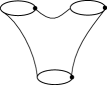
Figure 2. A representative of the one-point space $\mathcal{S}_{2,1}$ giving the pair of pants product.

Remark 5.1.

For families of spheres with more than two inputs, there ceases to be a preferred direction in which to point the asymptotic markers, a situation not considered in our work. However, if one mandates that all marked points lie on a single great circle, then one recovers the required preferred direction. The end result, which gives Massey products on $SH^{*}(M)$, will be constructed as a special case of the constructions in Sections 7 and 8.

5.2. $A_{\infty}$ structure maps and the wrapped Fukaya category

Here we define the higher structure maps $\mu^{k}$ on $\mathcal{W}$ (including the product $\mu^{2}$). We will recall and apply with some detail our construction of Floer-theoretic operations from Section 4.2, though the reader is warned that subsequent constructions will be more terse. Define

(5.2) $$\mathcal{R}^{d}$$

to be the (Stasheff) moduli space of discs with one negative marked point $z_{0}^{-}$ and $d$ positive marked points $z_{1}^{+},\ldots,z_{d}^{+}$ removed from the boundary, labeled in counterclockwise order from $z_{0}^{-}$. $\mathcal{R}^{d}$ is a special case of our general construction of open-closed strings. Denote by $\overline{\mathcal{R}}^{d}$ its natural (Deligne-Mumford) compactification, consisting of trees of stable discs with a total of $d$ exterior positive marked points and 1 exterior negative marked point, modulo compatible reparametrization of each disc in the tree. Recall from the discussion in Section 4 that $\overline{\mathcal{R}}^{d}$ inherits the structure of a manifold with corners, coming from standard gluing charts

(5.3) $$(0,+\infty]^{k}\times\sigma\rightarrow\overline{\mathcal{R}}^{d}.$$

near (nodal) strata of codimension $k$.

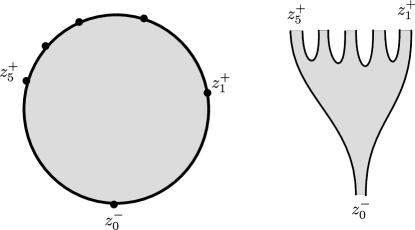
Figure 3. Two drawings of a representative of an element of the moduli space $\mathcal{R}^{5}$. The drawing on the right emphasizes the choices of strip-like ends.

Now, in the terminology of Definition 4.11, pick a universal and consistent choice of Floer data $\mathbf{D}_{\mu}$ for the spaces $\mathcal{R}^{d}$, $d>2$. Also, fix an orientation of the space $\mathcal{R}^{d}$, discussed in Appendix B.3.1.

Definition 5.2.

The $d$th order $A_{\infty}$ operation is by definition the operation

(5.4) $$\mu^{d}:=(-1)^{\vec{t}}\mathbf{F}_{\overline{\mathcal{R}}^{d}},$$

in the sense of (4.27), where $\vec{t}$ is the sign twisting datum given by $(1,2,\ldots,k)$.

We step through this construction for clarity. Let $L_{0},\ldots,L_{d}$ be objects of $\mathcal{W}$, and consider a sequence of chords $\vec{x}=\{x_{k}\in\chi(L_{k-1},L_{k})\}$ as well as another chord $x_{0}\in\chi(L_{0},L_{d})$. Given a fixed universal and consistent Floer data $\mathbf{D}_{\mu}$, write $\mathcal{R}^{d}(x_{0};\vec{x})$ for the space of maps

$$u:S\rightarrow M$$

with source an arbitrary element $S\in\mathcal{R}^{d}$, with marked points $(z^{0},\ldots,z^{d})$ satisfying the boundary asymptotic conditions

(5.5) $$\begin{cases}u(z)\in\psi^{a_{S}(z)}L_{k}&\mathrm{if\ }z\in\partial S\mathrm{\ lies\ between\ }z^{k}\ \mathrm{and\ }z^{k+1}\\ \lim_{s\rightarrow\pm\infty}u\circ\epsilon^{k}(s,\cdot)=\psi^{a_{S}(z)}x_{k}\end{cases}$$

and differential equation

(5.6) $$(du-X_{S}\otimes\alpha_{S})^{0,1}=0$$

with respect to the complex structure $J_{S}$ and total Hamiltonian $H_{S}+F_{S}$. Using the consistency of our Floer data and the codimension one boundary of the abstract moduli spaces $\overline{\mathcal{R}}^{d}$, Lemma 4.4 implies that the Gromov bordification $\overline{\mathcal{R}}^{d}(x_{0};\vec{x})$ is obtained by adding the images of the natural inclusions

(5.7) $$\overline{\mathcal{R}}^{d_{1}}(x_{0};\vec{x}_{1})\times\overline{\mathcal{R}}^{d_{2}}(y;\vec{x}_{2})\rightarrow\overline{\mathcal{R}}^{d}(x_{0};\vec{x})$$

where $y$ agrees with one of the elements of $\vec{x}_{1}$ and $\vec{x}$ is obtained by removing $y$ from $\vec{x}_{1}$ and replacing it with the sequence $\vec{x}_{2}$. Here, we let $d_{1}$ range from 1 to $d$, with $d_{2}=d-d_{1}+1$, with the stipulation that $d_{1}=$ or $d_{2}=1$ is the semistable case:

(5.8) $$\overline{\mathcal{R}}^{1}(x_{0};x_{1}):=\overline{\mathcal{R}}(x_{0};x_{1})$$

Thanks to Lemma 4.3, for generically chosen Floer data $\mathbf{D}_{\mu}$

Corollary 5.1.

The moduli spaces $\overline{\mathcal{R}}^{d}(x_{0};\vec{x})$ are smooth compact manifolds of dimension

$$\deg(x_{0})+d-2-\sum_{1\leq k\leq d}\deg(x_{k}).$$

In particular, if $\deg(x_{0})=2-d+\sum_{1}^{d}\deg(x_{k})$, then the elements of $\overline{\mathcal{R}}^{d}(x_{0};\vec{x})$ are rigid, and for any such rigid $u\in\overline{\mathcal{R}}^{d}(x_{0};\vec{x})$, we obtain by Lemma B.1, an isomorphism

(5.9) $$\mathcal{R}^{d}_{u}:o_{x_{d}}\otimes\cdots\otimes o_{x_{1}}\longrightarrow o_{x_{0}}.$$

Thus, taking into account the sign twisting $\vec{t}$, we define the operation

(5.10) $$\mu^{d}:CW^{*}(L_{d-1},L_{d})\otimes\cdots\otimes CW^{*}(L_{0},L_{1})\longrightarrow CW^{*}(L_{0},L_{d})$$

as a sum

(5.11) $$\mu^{d}([x_{d}],\ldots,[x_{1}]):=\sum_{\deg(x_{0})=2-d+\sum\deg(x_{k})}\sum_{u\in\overline{\mathcal{R}}^{d}(x_{0};\vec{x})}(-1)^{\bigstar_{d}}\mathcal{R}^{d}_{u}([x_{d}],\ldots,[x_{1}])$$

where

(5.12) $$\bigstar_{d}=\vec{t}\cdot\vec{\deg}(\vec{x}):=\sum_{i=1}^{d}i\cdot\deg(x_{i}).$$

By looking at the codimension 1 boundary of 1-dimensional families of such maps, and performing a tedious sign comparison analogous to those Appendix B (discussed in [Seidel:2008zr]*Prop. 12.3), we conclude that

Lemma 5.1.

The maps $\mu^{d}$ satisfy the $A_{\infty}$ relations.

The sign twisting datum used here will reappear with variations later, so it is convenient to fix notation.

Definition 5.3.

The incremental sign twisting datum of length $d$, denoted $\vec{t}_{d}$, is the vector $(1,2,\ldots,d-1,d)$.

5.3. From the open sector to the closed sector

As in [Abouzaid:2010kx], define $\mathcal{R}^{1}_{d}$ to be the abstract moduli space of discs with $d$ boundary positive punctures $z_{1},\ldots,z_{d}$ labeled in counterclockwise order and 1 interior negative puncture $z_{out}$, with the last positive puncture $x_{d}$ marked as distinguished. Its Deligne-Mumford compactification inherits the structure of a manifold with corners via the inclusion $\overline{\mathcal{R}}^{1}_{d}\hookrightarrow\overline{\mathcal{N}}_{h,n,\vec{m}}^{\mathbf{I},\vec{\mathbf{K}}}$ where $h=1$, $n=1$, $\vec{m}=(d)$, $\mathbf{I}=\{1\}$, $\vec{\mathbf{K}}=(\{\})$.

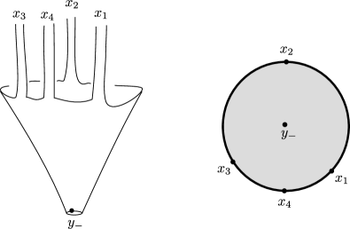
Figure 4. Two drawings of representative of an element of the moduli space $\mathcal{R}^{1}_{4}$. The drawing on the left emphasizes the choices of strip-like and cylindrical ends. The distinguished boundary marked point is the one set at $-i$ on the right.

In the manner of (4.19), using our fixed generic universal and consistent Floer data and an orientation for $\mathcal{R}^{1}_{d}$ fixed in Appendix B.3.2, we obtain, for every Lagrangian labeling $L_{1},\ldots,L_{d}$, and asymptotic conditions $\{x_{1},\ldots,x_{d},y_{out}\}$ moduli spaces

(5.13) $$\mathcal{R}^{1}_{d}(y_{out};\{x_{i}\})$$

which are compact smooth manifolds of dimension

(5.14) $$\deg(y_{out})-n+d-1-\sum_{k=0}^{d-1}\deg(x_{k}).$$

Then, fixing sign twisting datum

(5.15) $$\vec{t}_{\mathcal{OC},d}:=(1,2,\ldots,d-1,d+1)=\vec{t}_{d}+(0,\ldots,0,1),$$

we obtain associated operations

(5.16) $$\begin{split}\mathcal{OC}_{d}:=&(-1)^{\vec{t}_{\mathcal{OC},d}}\mathbf{F}_{\mathcal{R}^{1}_{d}}:\\ &\hom_{\mathcal{W}}(L_{d},L_{0})\otimes\hom_{\mathcal{W}}(L_{d-1},L_{d})\otimes\cdots\otimes\hom_{\mathcal{W}}(L_{0},L_{1})\longrightarrow CH^{*}(M);\end{split}$$

in other words, operations

(5.17) $$\mathcal{OC}_{d}:(\mathcal{W}_{\Delta}\otimes\mathcal{W}^{\otimes d-1})^{diag}\longrightarrow CH^{*}(M)$$

of degree $n-d+1$. The composite map

(5.18) $$\mathcal{OC}:=\sum_{d}\mathcal{OC}_{d}$$

therefore gives a map

(5.19) $$\mathcal{OC}:\mathrm{CC}_{*}(\mathcal{W},\mathcal{W})\longrightarrow CH^{*}(M)$$

of degree $n$ (using the grading conventions for Hochschild homology (2.174). Recall that the codimension-1 boundary of the Deligne-Mumford compactification $\overline{\mathcal{R}}^{1}_{d}$ is covered by the following strata:

(5.20) $$\overline{\mathcal{R}^{m}} \times_{i}\overline{\mathcal{R}}^{1}_{d-m+1}\ \ \ 1\leq i<d-m+1$$

(5.21) $$\overline{\mathcal{R}^{m}} \times_{d-m+1}\overline{\mathcal{R}}^{1}_{d-m+1}\ \ \ 1\leq j\leq m$$

where the notation $\times_{j}$ means that the output of the first component is identified with the $j$th boundary input of the second. In the second type of stratum (5.21), the $j$th copy correspond to the stratum in which the $j$th input point on $\mathcal{R}^{m}$ becomes the distinguished boundary marked point on $\mathcal{R}_{d}^{1}$ after gluing.

The consistency condition imposed on Floer data implies that the Gromov bordification $\overline{R}^{1}_{d}(y_{0},\vec{x})$ is obtained by adding the images of natural inclusions of moduli spaces of maps coming from the boundary strata (5.20)-(5.21) along with the following semi-stable breakings

(5.22) $$\mathcal{R}^{1}_{d}(y_{1},\vec{x})\times\mathcal{M}(y_{out};y_{1}) \rightarrow\partial\overline{\mathcal{R}}^{1}_{d}(y_{out};\vec{x})$$

(5.23) $$\overline{\mathcal{R}}^{1}(x_{1};x)\times\overline{\mathcal{R}}^{1}_{d}(y_{out};\tilde{\vec{x}}) \rightarrow\partial\overline{\mathcal{R}}^{1}_{d}(y_{out};\vec{x})$$

where in the second type of stratum, $x$ is one of the elements of $\vec{x}$ and $\tilde{\vec{x}}$ is the sequence obtained by replacing $x$ in $\vec{x}$ by $x_{1}$. Thus, modulo a tedious sign verification whose details are discussed in Appendix B, we obtain that

Proposition 5.1.

$\mathcal{OC}$ is a chain map.

5.4. From the closed sector to the open sector

In a similar fashion, define $\mathcal{R}^{1,1}_{d}$ to be the moduli space of discs with

• $d+1$ boundary marked points removed, $1$ of which is negative and labeled $z_{0}^{-}$, and $d$ of which are positive and labeled $(z_{1},\ldots,z_{d})$ in counterclockwise order from $z_{0}^{-}$; and

• one interior positive marked point $y_{in}$ removed.

Its Deligne-Mumford compactification inherits the structure of a manifold with corners via the inclusion $\overline{\mathcal{R}}^{1,1}_{d}\hookrightarrow\overline{\mathcal{N}}_{h,n,\vec{m}}^{\mathbf{I},\vec{\mathbf{K}}}$, where $h=1$, $n=1$, $\vec{m}=(d+1)$, $\mathbf{I}=\{\}$, $\vec{\mathbf{K}}=(\{1\})$. Thus, let us fix a universal and conformally consistent choice of Floer datum $\mathbf{D}_{\mathcal{CO}}$ on $\mathcal{R}^{1,1}_{d}$ for every $d\geq 1$. Given a Lagrangian labeling and a set of compatible asymptotic conditions, along with an orientation of $\mathcal{R}^{1,1}_{d}$ discussed in Appendix B.3.3, we obtain the moduli space $\mathcal{R}_{d}^{1,1}(x_{out};y_{in},\vec{x})$ as in (4.19), which are compact smooth manifolds of dimension

(5.24) $$\deg(x_{out})+d-\deg(y_{in})-\sum_{k=1}^{d}\deg(x_{k}).$$

Fix sign twisting datum

(5.25) $$\vec{t}_{\mathcal{CO},d}=(0,1,2,\ldots,d)$$

with respect to the ordering of inputs $(y_{in},x_{1},\ldots,x_{d})$. Then, define

(5.26) $$\mathcal{CO}_{d}:CH^{*}(M)\longrightarrow\hom_{Vect}(\mathcal{W}^{\otimes d},\mathcal{W})$$

as

(5.27) $$\mathcal{CO}_{d}(y_{in})(x_{d},\ldots,x_{1}):=(-1)^{\vec{t}_{\mathcal{CO},d}}\mathbf{F}_{\overline{\mathcal{R}}^{1,1}_{d}}(y_{in},x_{d},\ldots,x_{1})$$

The composite map

(5.28) $$\mathcal{CO}=\sum_{d}\mathcal{CO}_{d}$$

gives a map $CH^{*}(M)\rightarrow\mathrm{CC}^{*}(\mathcal{W},\mathcal{W})$.

The codimension-1 boundary of the Deligne-Mumford compactification $\overline{\mathcal{R}}^{1,1}_{d}$ is covered by the natural images of the following products:

(5.29) $$\overline{\mathcal{R}}^{m} \times_{i}\overline{\mathcal{R}}^{1,1}_{d-m+1}\ \ \ 1<m<d-1,\ 1\leq i<d-m+1$$

(5.30) $$\overline{\mathcal{R}}^{1,1}_{d-(k+l+1)+1} \times_{k+1}\overline{\mathcal{R}}^{k+l+1}\ \ 0<k+l<d-1.$$

using the notation $\times_{j}$ as in the last section to indicate gluing the distinguished output of the first component to the $j$th (boundary) input of the second component.

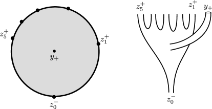
Figure 5. Two drawings of representative of an element of the moduli space $\mathcal{R}^{1,1}_{5}$. The drawing on the right emphasizes the choices of strip-like and cylindrical ends.

The consistency condition implies that the Gromov bordification $\mathcal{\overline{R}}^{1,1}_{d}(x_{out};y_{in},\vec{x})$ is obtained by adding images of the natural inclusions

(5.31) $$\mathcal{M}(y_{1};y_{in})\times\mathcal{R}^{1,1}_{d}(x_{out};y_{1},\vec{x}) \rightarrow\partial\overline{\mathcal{R}}^{1,1}_{d}(x_{out};y_{in},\vec{x})$$

(5.32) $$\mathcal{R}^{1,1}_{d_{2}}(x^{a};y_{in},\vec{x}^{2})\times\mathcal{R}^{d_{1}}(x_{out},\vec{x}^{1}) \rightarrow\partial\overline{\mathcal{R}}^{1,1}_{d}(x_{out};y_{in},\vec{x})$$

(5.33) $$\mathcal{R}^{d_{2}}(x^{a};\vec{x}^{2})\times\mathcal{R}^{1,1}_{d_{1}}(x_{out};y_{in},\vec{x}^{1}) \rightarrow\partial\overline{\mathcal{R}}^{1,1}_{d}(x_{out};y_{in},\vec{x})$$

where $d_{1}+d_{2}-1=d$, $\vec{x}^{2}$ is any consecutive sub-vector of size $d_{2}$ and $\vec{x}^{1}$ is obtained by replacing $\vec{x}^{2}$ in $\vec{x}$ by $x^{a}$. By the above result about Gromov bordification, and a sign verification discussed in Appendix B, we see that:

Proposition 5.2.

$\mathcal{CO}$ is a chain map.

5.5. Ring and module structure compatibility

We will make two assertions about the maps $\mathcal{CO}$ and $\mathcal{OC}$, both of which follow from an analysis of similar-looking moduli spaces.

Proposition 5.3.

$[\mathcal{CO}]$ is a ring homomorphism.

Via its module structure over Hochschild cohomology and the ring homomorphism $[\mathcal{CO}]$, Hochschild homology $\mathrm{HH}_{*}(\mathcal{W},\mathcal{W})$ obtains the structure of a module over $SH^{*}(M)$. With respect to this structure, using a similar argument, we can prove the following:

Proposition 5.4.

$[\mathcal{OC}]$ is a map of $SH^{*}(M)$-modules.

The chain-level statement is that the following diagram homotopy commutes:

(5.34) $$\lx@xy@svg{\hbox{\raise 0.0pt\hbox{\kern 45.93956pt\hbox{\ignorespaces\ignorespaces\ignorespaces\hbox{\vtop{\kern 0.0pt\offinterlineskip\halign{\entry@#!@&&\entry@@#!@\cr&\\&\crcr}}}\ignorespaces{\hbox{\kern-45.93956pt\raise 0.0pt\hbox{\hbox{\kern 0.0pt\raise 0.0pt\hbox{\hbox{\kern 3.0pt\raise 0.0pt\hbox{$\textstyle{\mathrm{CC}_{*}(\mathcal{W})\times CH^{*}(M)\ignorespaces\ignorespaces\ignorespaces\ignorespaces\ignorespaces\ignorespaces\ignorespaces\ignorespaces}$}}}}}}}\ignorespaces\ignorespaces\ignorespaces\ignorespaces{}{\hbox{\lx@xy@droprule}}\ignorespaces\ignorespaces\ignorespaces{\hbox{\kern 43.84264pt\raise 6.5pt\hbox{{}\hbox{\kern 0.0pt\raise 0.0pt\hbox{\hbox{\kern 3.0pt\hbox{\hbox{\kern 0.0pt\raise-1.75pt\hbox{$\scriptstyle{(\mathcal{OC},\mathrm{id})}$}}}\kern 3.0pt}}}}}}\ignorespaces{\hbox{\kern 69.93956pt\raise 0.0pt\hbox{\hbox{\kern 0.0pt\raise 0.0pt\hbox{\lx@xy@tip{1}\lx@xy@tip{-1}}}}}}{\hbox{\lx@xy@droprule}}{\hbox{\lx@xy@droprule}}\ignorespaces\ignorespaces\ignorespaces\ignorespaces{}{\hbox{\lx@xy@droprule}}\ignorespaces\ignorespaces\ignorespaces{\hbox{\kern 0.0pt\raise-20.31804pt\hbox{{}\hbox{\kern 0.0pt\raise 0.0pt\hbox{\hbox{\kern 3.0pt\hbox{\hbox{\kern 0.0pt\raise-1.75pt\hbox{$\scriptstyle{(\mathrm{id},\mathcal{CO})}$}}}\kern 3.0pt}}}}}}\ignorespaces{\hbox{\kern 0.0pt\raise-29.49998pt\hbox{\hbox{\kern 0.0pt\raise 0.0pt\hbox{\lx@xy@tip{1}\lx@xy@tip{-1}}}}}}{\hbox{\lx@xy@droprule}}{\hbox{\lx@xy@droprule}}{\hbox{\kern 69.93956pt\raise 0.0pt\hbox{\hbox{\kern 0.0pt\raise 0.0pt\hbox{\hbox{\kern 3.0pt\raise 0.0pt\hbox{$\textstyle{CH^{*}(M)\times CH^{*}(M)\ignorespaces\ignorespaces\ignorespaces\ignorespaces}$}}}}}}}\ignorespaces\ignorespaces\ignorespaces\ignorespaces{}{\hbox{\lx@xy@droprule}}\ignorespaces\ignorespaces\ignorespaces{\hbox{\kern 117.40755pt\raise-20.31804pt\hbox{{}\hbox{\kern 0.0pt\raise 0.0pt\hbox{\hbox{\kern 3.0pt\hbox{\hbox{\kern 0.0pt\raise-1.62848pt\hbox{$\scriptstyle{*}$}}}\kern 3.0pt}}}}}}\ignorespaces{\hbox{\kern 117.40755pt\raise-29.49998pt\hbox{\hbox{\kern 0.0pt\raise 0.0pt\hbox{\lx@xy@tip{1}\lx@xy@tip{-1}}}}}}{\hbox{\lx@xy@droprule}}{\hbox{\lx@xy@droprule}}{\hbox{\kern-43.30005pt\raise-40.63608pt\hbox{\hbox{\kern 0.0pt\raise 0.0pt\hbox{\hbox{\kern 3.0pt\raise 0.0pt\hbox{$\textstyle{\mathrm{CC}_{*}(\mathcal{W})\times\mathrm{CC}^{*}(\mathcal{W})\ignorespaces\ignorespaces\ignorespaces\ignorespaces}$}}}}}}}\ignorespaces\ignorespaces\ignorespaces\ignorespaces{}{\hbox{\lx@xy@droprule}}\ignorespaces\ignorespaces\ignorespaces{\hbox{\kern 42.87044pt\raise-35.24442pt\hbox{{}\hbox{\kern 0.0pt\raise 0.0pt\hbox{\hbox{\kern 3.0pt\hbox{\hbox{\kern 0.0pt\raise-2.39166pt\hbox{$\scriptstyle{\mbox{ }\mbox{ }\mbox{ }\mathcal{OC}\circ\cap}$}}}\kern 3.0pt}}}}}}\ignorespaces{\hbox{\kern 95.2291pt\raise-40.63608pt\hbox{\hbox{\kern 0.0pt\raise 0.0pt\hbox{\lx@xy@tip{1}\lx@xy@tip{-1}}}}}}{\hbox{\lx@xy@droprule}}{\hbox{\lx@xy@droprule}}{\hbox{\kern 95.2291pt\raise-40.63608pt\hbox{\hbox{\kern 0.0pt\raise 0.0pt\hbox{\hbox{\kern 3.0pt\raise 0.0pt\hbox{$\textstyle{CH^{*}(M)}$}}}}}}}\ignorespaces}}}}\ignorespaces, \textstyle{\mathrm{CC}_{*}(\mathcal{W})\times CH^{*}(M)\ignorespaces\ignorespaces\ignorespaces\ignorespaces\ignorespaces\ignorespaces\ignorespaces\ignorespaces} \scriptstyle{(\mathcal{OC},\mathrm{id})} \scriptstyle{(\mathrm{id},\mathcal{CO})} \textstyle{CH^{*}(M)\times CH^{*}(M)\ignorespaces\ignorespaces\ignorespaces\ignorespaces} \scriptstyle{*} \textstyle{\mathrm{CC}_{*}(\mathcal{W})\times\mathrm{CC}^{*}(\mathcal{W})\ignorespaces\ignorespaces\ignorespaces\ignorespaces} \scriptstyle{\mbox{ }\mbox{ }\mbox{ }\mathcal{OC}\circ\cap} \textstyle{CH^{*}(M)} \textstyle{\mathrm{CC}_{*}(\mathcal{W})\times CH^{*}(M)\ignorespaces\ignorespaces\ignorespaces\ignorespaces\ignorespaces\ignorespaces\ignorespaces\ignorespaces} \scriptstyle{(\mathcal{OC},\mathrm{id})} \scriptstyle{(\mathrm{id},\mathcal{CO})} \textstyle{CH^{*}(M)\times CH^{*}(M)\ignorespaces\ignorespaces\ignorespaces\ignorespaces} \scriptstyle{*} \textstyle{\mathrm{CC}_{*}(\mathcal{W})\times\mathrm{CC}^{*}(\mathcal{W})\ignorespaces\ignorespaces\ignorespaces\ignorespaces} \scriptstyle{\mbox{ }\mbox{ }\mbox{ }\mathcal{OC}\circ\cap} \textstyle{CH^{*}(M)}$$

To prove Proposition 5.34, for $r\in(0,1)$, define the auxiliary moduli space

(5.35) $$\mathcal{P}^{2}_{d}(r)$$

to consist of the unit disc in ${\mathbb{C}}$ with the following data:

• $d+1$ positive boundary marked points $(z_{0},\ldots,z_{d})$, with $z_{d}$ marked as distinguished, and

• two interior marked points $(\kappa_{+},\kappa_{-})$, one positive and one negative

such that,

(5.36) $$\textrm{after automorphism, the points $z_{d}$, $\kappa_{+}$, $\kappa_{-}$ lie at $-i$, $-r$, and $r$ respectively}.$$

These spaces vary smoothly with $r$ and their union

(5.37) $$\mathcal{P}^{2}_{d}:=\bigcup_{r\in(0,1)}\mathcal{P}^{2}_{d}(r)$$

is naturally a codimension 1 submanifold of genus 0 open-closed strings consisting of a single disc with $d$ positive boundary punctures and two interior punctures, one positive and one negative. Compactifying, we obtain a family that submerses over $r\in[0,1]$ and see that with codimension-1 boundary of $\overline{\mathcal{P}}^{2}_{d}$ is covered by the images of the natural inclusions of the following products (some living over the endpoints $r\in\{0,1\}$ and some living over the entire interval):

(5.38) $$\overline{\mathcal{R}}^{1,1}_{d_{3}}\times_{n+k+1}\overline{\mathcal{R}}^{k+1+d_{2}} \times_{m}\overline{\mathcal{R}}^{1}_{d+1-d_{3}-d_{2}-k},\ \ \ d_{1}+d_{2}+d_{3}-2=d\ \ \ (r=1)$$

(5.39) $$\overline{\mathcal{R}}^{1}_{d+1} \times_{2}\overline{\mathcal{S}}_{2}\ \ \ \ (r=0)$$

(5.40) $$\overline{\mathcal{R}}^{m} \times_{n}\overline{\mathcal{P}}^{2}_{d-m+1}$$

(5.41) $$\overline{\mathcal{R}}^{m} \times_{d-m+1}\overline{\mathcal{P}}^{2}_{d-m+1}.$$

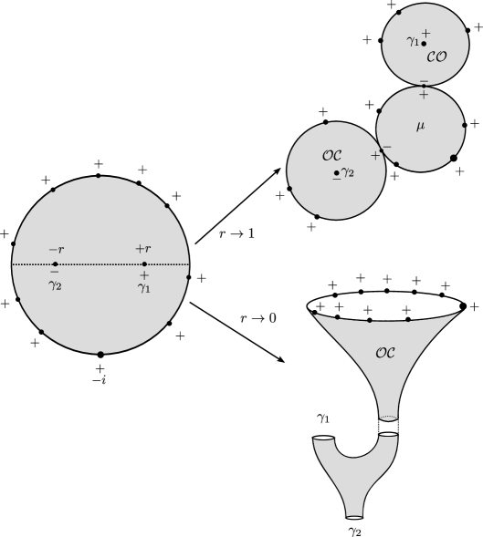
Figure 6. The space $\mathcal{P}^{2}_{d}$ and its $r\rightarrow\{0,1\}$ degenerations. Not shown in the degeneration: the special input point is constrained to remain on the middle $\mu$ bubble.

Fix a universal and consistent Floer data for all $\overline{\mathcal{P}}^{2}_{d}$. Given a set of Lagrangian labels

(5.42) $$L_{0},\ldots,L_{d},L_{d+1}=L_{0}$$

and compatible asymptotic conditions $\vec{x}=\{x_{k}\in\mathcal{X}(L_{k},L_{k+1})\}_{k=0}^{d}$ and $\gamma_{-},\gamma_{+}$, we obtain a moduli space of maps

(5.43) $$\mathcal{P}^{2}_{d}(\gamma_{-};\gamma_{+},\vec{x}).$$

which are smooth compact manifolds of dimension

(5.44) $$\deg(\gamma_{-})-n+d+1-\deg(\gamma_{+})-\sum_{k=0}^{d}\deg(x_{k}).$$

Consistency of our Floer data implies that the Gromov bordification $\overline{\mathcal{P}}^{2}_{d}(\gamma_{-};\gamma_{+},\vec{x})$ is obtained by adding the images of the natural inclusions

(5.45) $$\mathcal{M}(\gamma_{0};\gamma_{+})\times\overline{\mathcal{P}}^{2}_{d}(\gamma_{-};\gamma_{0},\vec{x}) \rightarrow\partial\overline{\mathcal{P}}^{2}_{d}(\gamma_{-};\gamma_{+},\vec{x})$$

(5.46) $$\overline{\mathcal{P}}^{2}_{d}(\gamma_{0};\gamma_{+},\vec{x})\times\mathcal{M}(\gamma_{-};\gamma_{0}) \rightarrow\partial\overline{\mathcal{P}}^{2}_{d}(\gamma_{-};\gamma_{+},\vec{x})$$

(5.47) $$\overline{\mathcal{R}}^{d_{1}}(x_{a};\vec{x}^{2})\times\overline{\mathcal{P}}^{2}_{d_{2}}(\gamma_{-};\gamma_{+},\vec{x}^{1}) \rightarrow\partial\overline{\mathcal{P}}^{2}_{d}(\gamma_{-};\gamma_{+},\vec{x})$$

(5.48) $$\overline{\mathcal{R}}^{1}_{d}(\gamma_{1};\vec{x})\times\overline{\mathcal{S}}_{2}(\gamma_{-};\gamma_{+},\gamma_{1}) \rightarrow\partial\overline{\mathcal{P}}^{2}_{d}(\gamma_{-};\gamma_{+},\vec{x})$$

(5.49) $$\overline{\mathcal{R}}^{1,1}_{d_{3}}(x_{b};\gamma_{+},\vec{x}^{3})\times\overline{\mathcal{R}}_{d_{2}}(x_{a};\vec{x}^{2})\times\overline{\mathcal{R}}^{1}_{d_{1}}(\gamma_{-};\vec{x}^{1}) \rightarrow\partial\overline{\mathcal{P}}^{2}_{d}(\gamma_{-};\gamma_{+},\vec{x})$$

where

• in (5.47), $\vec{x}^{2}$ is a subvector of $\vec{x}$, and $\vec{x}^{1}$ is obtained from $\vec{x}$ by replacing $\vec{x}^{2}$ by $x_{a}$

• in (5.49), $\vec{x}^{3}$ is a subvector of $\vec{x}$, not including the distinguished input $x_{0}$. $\widehat{\vec{x}^{2}}$ is obtained from $\vec{x}$ by replacing $\vec{x}^{3}$ by $x_{b}$, and then performing a cyclic permutation that brings the distinguished output $x_{0}$ to the right of $x_{b}$. $\vec{x}^{2}$ is a subvector of $\widehat{\vec{x}}^{2}$ that includes both $x_{b}$ and $x_{0}$, and $\vec{x}^{1}$ is obtained from $\widehat{\vec{x}}^{2}$ by replacing $\vec{x}^{2}$ with $x_{a}$.

Now, define the map

(5.50) $$\mathcal{H}_{d}:CH^{*}(M)\otimes(\mathcal{W}_{\Delta}\otimes\mathcal{W}^{\otimes d})^{diag}\rightarrow CH^{*}(M)$$

as

(5.51) $$\mathcal{H}_{d}:=(-1)^{\vec{t}_{\mathcal{P}^{2}_{d}}}\mathbf{F}_{\overline{\mathcal{P}}^{2}_{d}},$$

where we use sign twisting datum

(5.52) $$\vec{t}_{\mathcal{P}^{2}_{d}}:=(-1,0,1,\ldots,d)$$

corresponding to the ordering of inputs $(\kappa_{+},z_{0},\ldots,z_{d})$. The composite map $\mathcal{H}=\sum_{d}\mathcal{H}_{d}$ gives a map

(5.53) $$\mathcal{H}:CH^{*}(M)\times\mathrm{CC}_{*}(\mathcal{W},\mathcal{W})\longrightarrow CH^{*}(M).$$

By the above result about Gromov bordifications and a sign verification discussed in Appendix B we conclude that

Proposition 5.5.

For any $\alpha,s\in\mathrm{CC}_{*}(\mathcal{W}),CH^{*}(M)$,

(5.54) $$d_{SH}\circ\mathcal{H}(\alpha,s)\pm\mathcal{H}(\delta(\alpha),s)\pm\mathcal{H}(\alpha,d_{SH}(s))=\mathcal{OC}(\alpha)*s-\mathcal{OC}(\mathcal{CO}(s)\cap\alpha).$$

Thus, $\mathcal{H}$ is the desired chain homotopy for (5.34), concluding the proof of Proposition 5.4. We briefly indicate how to change this argument to prove Proposition 5.3. One considers operation associated to the same abstract moduli space as $\mathcal{P}^{2}_{d}$, where both interior punctures are marked as positive points and the distinguished boundary input is now marked as an output. The associated Floer theoretic operation with a similar sign twist gives a homotopy between the Yoneda product applied to elements of $\mathcal{CO}$ (the degenerate limit $r\rightarrow 1$) and the pair of pants product applied before applying $\mathcal{CO}$ (the limit $r\rightarrow 0$).

Proof of Proposition 1.1.

Suppose $M$ is non-degenerate, and let $\sigma$ be any homology level pre-image of $1\in SH^{*}(M)$ via the map $\mathcal{OC}$. Then, if $s$ is another element of $SH^{*}(M)$, we see that by Proposition 5.4, on homology

(5.55) $$\mathcal{OC}(\mathcal{CO}(s)\cap\sigma)=s\cdot\mathcal{OC}(\sigma)=s\cdot 1=1.$$

In particular this implies that $\mathcal{CO}(s)\cap\sigma$ is a preimage of $s$, and $\mathcal{CO}(s)$ cannot be zero unless $s$ is. ∎

5.6. Two-pointed open-closed maps

Since the two-pointed complexes

$${{}_{2}}\mathrm{CC}_{*}(\mathcal{W},\mathcal{W}),\ {{}_{2}}\mathrm{CC}^{*}(\mathcal{W},\mathcal{W})$$

arise naturally from a bimodule perspective, we will define variants of the chain-level map $\mathcal{OC}$ and $\mathcal{CO}$ between $SH^{*}(M)$ and the respective two-pointed complexes:

(5.56) $${{}_{2}}\mathcal{OC}:{{}_{2}}\mathrm{CC}_{*}(\mathcal{W},\mathcal{W}) \longrightarrow SH^{*}(M)$$

(5.57) $${{}_{2}}\mathcal{CO}:SH^{*}(M) \longrightarrow{{}_{2}}\mathrm{CC}^{*}(\mathcal{W},\mathcal{W})$$

To ensure consistency with existing arguments, we prove that the resulting maps are in fact quasi-isomorphic to $\mathcal{OC}$ and $\mathcal{CO}$.

Definition 5.4.

The two-pointed open-closed moduli space with $(k,l)$ marked points

(5.58) $$\mathcal{R}^{1}_{k,l}$$

is the space of discs with one interior negative puncture labeled $y_{out}$, and $k+l+2$ boundary punctures, labeled in counterclockwise order $z_{0},z_{1},\ldots,z_{k},z_{0}^{\prime},z_{1}^{\prime},\ldots,z_{l}^{\prime}$, such that:

(5.59) $$\textrm{up to automorphism, }z_{0},\ z_{0}^{\prime},\ \textrm{and }y_{out}\ \textrm{are constrained to lie at }-i,\ i\ \textrm{and }0\textrm{ respectively}.$$

Call $z_{0}$ and $z_{0}^{\prime}$ the special inputs of any such disc.

Remark 5.2.

The moduli space $\mathcal{R}^{1}_{k,l}$ is a codimension one submanifold of $\mathcal{R}^{1}_{k+l+2}$, and thus has dimension $k+l$.

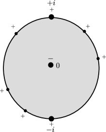
Figure 7. A representative of an element of the moduli space $\mathcal{R}^{1}_{3,2}$ with special points at 0 (output), $-i$, and $i$.

The boundary strata of Deligne-Mumford compactification $\overline{\mathcal{R}}^{1}_{k,l}$ is covered by the images of the natural inclusions of the following products:

(5.60) $$\overline{\mathcal{R}}^{k^{\prime}} \times_{n+1}\overline{\mathcal{R}}^{1}_{k-k^{\prime}+1,l},\ \ \ 0\leq n<k-k^{\prime}+1$$

(5.61) $$\overline{\mathcal{R}}^{l^{\prime}} \times_{(n+1)^{\prime}}\overline{\mathcal{R}}^{1}_{k,l-l^{\prime}+1},\ \ \ 0\leq n^{\prime}<l-l^{\prime}+1$$

(5.62) $$\overline{\mathcal{R}}^{k^{\prime}+l^{\prime}+1} \times_{0}\overline{\mathcal{R}}^{1}_{k-k^{\prime},l-l^{\prime}}$$

(5.63) $$\overline{\mathcal{R}}^{l^{\prime}+k^{\prime}+1} \times_{0^{\prime}}\overline{\mathcal{R}}^{1}_{k-k^{\prime},l-l^{\prime}}.$$

Here the notation $\times_{j}$ indicates that one glues the distinguished output of the first factor to the input $z_{j}$, and the notation $\times_{j^{\prime}}$ indicates that one glues the distinguished output of the first factor to the input $z_{j}^{\prime}$. Moreover, in (5.62), after gluing the output of the first disc to to the first special point $z_{0}$, the $k^{\prime}+1$st input becomes the new special point $z_{0}$. Similarly in (5.63), after gluing the output of the first stable disc to the second special point $z_{0}^{\prime}$, the $l^{\prime}+1$st input becomes the new special point $z_{0}^{\prime}$. Thinking of $\mathcal{R}^{1}_{k,l}$ as a submanifold of open-closed strings, we obtain, given a compatible Lagrangian labeling $\{L_{0},\ldots,L_{k},L_{0}^{\prime},\ldots,L_{l}^{\prime}\}$ asymptotic input chords $\{x_{0},x_{1},\ldots,x_{k},x_{0}^{\prime},x_{1}^{\prime},\ldots,x_{l}^{\prime}\}$ and output orbit $y$, Floer theoretic moduli spaces

(5.64) $$\overline{\mathcal{R}}^{1}_{k,l}(y;x_{0},x_{1},\ldots,x_{k},x_{0}^{\prime},x_{1}^{\prime},\ldots,x_{l}^{\prime})$$

of dimension

(5.65) $$k+l-n+\deg(y)-\deg(x_{0})-\deg(x_{0}^{\prime})-\sum_{i=1}^{k}\deg(x_{i})-\sum_{j=1}^{l}\deg(x_{j}^{\prime}).$$

Here, $L_{k},L_{0}^{\prime}$ are adjacent to the second special point $z_{0}^{\prime}$ and $L_{l}^{\prime},L_{0}$ are adjacent to $z_{0}$ (with corresponding inputs $x_{0}^{\prime},x_{0}$). Using the sign twisting datum

(5.66) $$\vec{t}_{{}_{2}\mathcal{OC}_{k,l}}=(1,2,\ldots,k+1,k+3,k+4,\ldots,k+2+l)$$

with respect to the ordering of inputs $(z_{0},\ldots,z_{k},z_{0}^{\prime},\ldots,z_{l}^{\prime})$, define associated Floer-theoretic operations

(5.67) $${}_{2}\mathcal{OC}_{k,l}:=(-1)^{\vec{t}_{{}_{2}\mathcal{OC}}}\mathbf{F}_{\overline{\mathcal{R}}^{1}_{k,l}}:(\mathcal{W}_{\Delta}\otimes\mathcal{W}^{\otimes l}\otimes\mathcal{W}_{\Delta}\otimes\mathcal{W}^{\otimes k})^{diag}\longrightarrow CH^{*}(M).$$

The two-pointed open-closed map is defined to be the sum of these operations:

(5.68) $${}_{2}\mathcal{OC}=\sum_{k,l}{{}_{2}}\mathcal{OC}_{k,l}:(\mathcal{W}_{\Delta}\otimes T\mathcal{W}\otimes\mathcal{W}_{\Delta}\otimes T\mathcal{W})^{diag}\longrightarrow CH^{*}(M).$$

With respect to the grading on the 2-pointed Hochschild complex, ${}_{2}\mathcal{OC}$ is once more a map of degree $n$. By analyzing the boundary of the one-dimensional components of $\overline{\mathcal{R}}^{1}_{k,l}$, seeing that the relevant boundary behavior is governed by the codimension-1 boundary of the abstract moduli space $\overline{\mathcal{R}}^{1}_{k,l}$ described from (5.60)-(5.63) and strip-breaking, and performing a sign verification in Appendix B, we conclude that

Corollary 5.2.

The map ${}_{2}\mathcal{OC}:{{}_{2}}\mathrm{CC}_{*}(\mathcal{W},\mathcal{W})\longrightarrow CH^{*}(M)$ is a chain map.

Definition 5.5.

The two-pointed closed-open moduli space with $(r,s)$ marked points

(5.69) $$\mathcal{R}^{1,1}_{r,s}$$

is the space of discs with one interior positive puncture labeled $y_{in}$, one negative boundary puncture $z_{out}$, and $r+s+1$ positive boundary punctures, labeled in clockwise order from $z_{out}$ as $z_{1},\ldots,z_{r},z_{fixed},z_{1}^{\prime},\ldots,z_{s}^{\prime}$, subject to the following constraint:

(5.70) $$\textrm{up to automorphism, }z_{out},\ z_{fixed},\ \textrm{and }y_{in}\ \textrm{lie at }-i,\ i\ \textrm{and }0\textrm{ respectively}.$$

The boundary strata of the Deligne-Mumford compactification $\overline{\mathcal{R}}^{1,1}_{r,s}$ is covered by the natural inclusions of the following products:

(5.71) $$\overline{\mathcal{R}}^{r^{\prime}} \times_{n+1}\overline{\mathcal{R}}^{1,1}_{r-r^{\prime}+1,s},\ \ \ 0\leq n<r-r^{\prime}+1$$

(5.72) $$\overline{\mathcal{R}}^{s^{\prime}} \times_{(m+1)^{\prime}}\overline{\mathcal{R}}^{1,1}_{r,s-s^{\prime}+1},\ \ \ 0\leq m<s-s^{\prime}+1$$

(5.73) $$\overline{\mathcal{R}}^{r^{\prime}+s^{\prime}+1} \times_{0}\overline{\mathcal{R}}^{1,1}_{r-r^{\prime},s-s^{\prime}}$$

(5.74) $$\overline{\mathcal{R}}^{1,1}_{r-a^{\prime},s-b^{\prime}} \times_{a^{\prime}+1}\overline{\mathcal{R}}^{a^{\prime}+b^{\prime}+1}.$$

Here in (5.73), the output of the stable disc is glued to the special input $z_{fixed}$ with the $r^{\prime}+1$st point becoming the new distinguished $z_{fixed}$. Similarly, in (5.74), the output of the two-pointed closed-open disc $z_{out}$ is glued to the $a+1$st input of the stable disc.

Thinking of $\mathcal{R}^{1,1}_{r,s}$ as a submanifold of open-closed strings, we obtain, given a compatible Lagrangian labeling

(5.75) $$\{L_{0},\ldots,L_{r},L_{0}^{\prime},\ldots,L_{s}^{\prime}\}$$

and input chords $\{x_{1},\ldots,x_{r},x_{fixed},x_{1}^{\prime},\ldots,x_{s}^{\prime}\}$ input orbit $y$, and output chord $x_{out}$, a moduli space

(5.76) $$\overline{\mathcal{R}}^{1,1}_{r,s}(x_{out};y,x_{1},\ldots,x_{r},x_{fixed},x_{1}^{\prime},\ldots,x_{s}^{\prime})$$

of dimension

(5.77) $$r+s+\deg(x_{out})-\deg(y)-\deg(x_{fixed})-\sum_{i=1}^{r}\deg(x_{i})-\sum_{j=1}^{s}\deg(x_{j}^{\prime}).$$

Here, $L_{r},L_{0}^{\prime}$ are adjacent to the second special output $z_{out}$ and $L_{s}^{\prime},L_{0}$ are adjacent to $z_{fixed}$ (with corresponding asymptotic conditions $x_{out},x_{fixed}$). We also obtain associated Floer-theoretic operations

(5.78) $$\mathbf{F}_{\overline{\mathcal{R}}^{1,1}_{r,s}}:CH^{*}(M)\otimes(\mathcal{W}^{\otimes s}\otimes\mathcal{W}_{\Delta}\otimes\mathcal{W}^{\otimes r})\longrightarrow\mathcal{W}_{\Delta}.$$

Now, define

(5.79) $${}_{2}\mathcal{CO}_{r,s}:CH^{*}(M)\longrightarrow\hom_{Vect}(\mathcal{W}^{\otimes s}\otimes\mathcal{W}_{\Delta}\otimes\mathcal{W}^{\otimes r},\mathcal{W}_{\Delta})$$

as

(5.80) $${}_{2}\mathcal{CO}_{r,s}(y)(y_{s},\ldots,y_{1},\mathbf{b},x_{s},\ldots,x_{1}):=(-1)^{\vec{t}_{{}_{2}\mathcal{CO}_{r,s}}}\mathbf{F}_{\overline{\mathcal{R}}^{1,1}_{r,s}}(y,y_{s},\ldots,x_{1},\mathbf{b},x_{r},\ldots,x_{1})$$

where $\vec{t}_{{}_{2}\mathcal{CO}_{r,s}}$ is the sign twisting datum

(5.81) $$\vec{t}_{{}_{2}\mathcal{CO}_{r,s}}:=(-1,0,\ldots,r-1,r+1,r+2,\ldots,r+s+1)$$

with respect to the input ordering $(y_{in},z_{1},\ldots,z_{r},z_{fixed},z_{1}^{\prime},\ldots,z_{s}^{\prime})$. Define the two-pointed closed-open map to be the sum of these operations

(5.82) $${{}_{2}}\mathcal{CO}=\sum_{r,s}{{}_{2}}\mathcal{CO}_{r,s}:CH^{*}(M)\longrightarrow\hom_{\mathcal{W}\!-\!\mathcal{W}}(\mathcal{W}_{\Delta},\mathcal{W}_{\Delta})$$

With respect to the grading on the 2-pointed Hochschild co-chain complex, ${}_{2}\mathcal{CO}$ is once more a map of degree $0$. An analysis of the boundary of the one-dimensional components of $\overline{\mathcal{R}}^{1,1}_{k,l}$ coming from strip-breaking and the codimension-1 boundary of the abstract moduli space $\overline{\mathcal{R}}^{1,1}_{k,l}$ described in (5.71)-(5.74), along with a sign verification discussed in Appendix B, we conclude that

Corollary 5.3.

The map ${}_{2}\mathcal{CO}:CH^{*}(M)\longrightarrow{{}_{2}}\mathrm{CC}^{*}(\mathcal{W},\mathcal{W})$ is a chain map.

We remark that the quasi-isomorphisms of chain complexes

$$\begin{split}\mathbf{\Phi}:{{}_{2}}\mathrm{CC}_{*}(\mathcal{W},\mathcal{W})&\stackrel{{\scriptstyle\sim}}{{\longrightarrow}}\mathrm{CC}_{*}(\mathcal{W},\mathcal{W})\\ \mathbf{\Psi}:\mathrm{CC}^{*}(\mathcal{W},\mathcal{W})&\stackrel{{\scriptstyle\sim}}{{\longrightarrow}}{{}_{2}}\mathrm{CC}^{*}(\mathcal{W},\mathcal{W})\end{split}$$

defined in (2.196) and (2.201) induce identifications of the two-pointed open-closed maps with the usual open-closed maps. The precise statement is:

Proposition 5.6.

There are homotopy-commutative diagrams

(5.83)

and

(5.84) $$\lx@xy@svg{\hbox{\raise 0.0pt\hbox{\kern 27.17783pt\hbox{\ignorespaces\ignorespaces\ignorespaces\hbox{\vtop{\kern 0.0pt\offinterlineskip\halign{\entry@#!@&&\entry@@#!@\cr&\\&\crcr}}}\ignorespaces{\hbox{\kern-21.60136pt\raise 0.0pt\hbox{\hbox{\kern 0.0pt\raise 0.0pt\hbox{\hbox{\kern 3.0pt\raise 0.0pt\hbox{$\textstyle{SH^{*}(M)\ignorespaces\ignorespaces\ignorespaces\ignorespaces\ignorespaces\ignorespaces\ignorespaces\ignorespaces}$}}}}}}}\ignorespaces\ignorespaces\ignorespaces{}\ignorespaces\ignorespaces{\hbox{\lx@xy@drawline@}}\ignorespaces\ignorespaces\ignorespaces{\hbox{\kern 35.34315pt\raise-14.28194pt\hbox{{}\hbox{\kern 0.0pt\raise 0.0pt\hbox{\hbox{\kern 3.0pt\hbox{\hbox{\kern 0.0pt\raise-1.74722pt\hbox{$\scriptstyle{{{}_{2}}\mathcal{CO}}$}}}\kern 3.0pt}}}}}}\ignorespaces{\hbox{\kern 57.9076pt\raise-29.49998pt\hbox{\hbox{\kern 0.0pt\raise 0.0pt\hbox{\lx@xy@tip{1}\lx@xy@tip{-1}}}}}}\ignorespaces\ignorespaces{\hbox{\lx@xy@drawline@}}\ignorespaces{\hbox{\lx@xy@drawline@}}\ignorespaces\ignorespaces\ignorespaces\ignorespaces{}{\hbox{\lx@xy@droprule}}\ignorespaces\ignorespaces\ignorespaces{\hbox{\kern 0.0pt\raise-20.31804pt\hbox{{}\hbox{\kern 0.0pt\raise 0.0pt\hbox{\hbox{\kern 3.0pt\hbox{\hbox{\kern 0.0pt\raise-2.39166pt\hbox{$\scriptstyle{\mathcal{CO}}$}}}\kern 3.0pt}}}}}}\ignorespaces{\hbox{\kern 0.0pt\raise-29.49998pt\hbox{\hbox{\kern 0.0pt\raise 0.0pt\hbox{\lx@xy@tip{1}\lx@xy@tip{-1}}}}}}{\hbox{\lx@xy@droprule}}{\hbox{\lx@xy@droprule}}{\hbox{\kern 76.75565pt\raise 0.0pt\hbox{\hbox{\kern 0.0pt\raise 0.0pt\hbox{\hbox{\kern 3.0pt\raise 0.0pt\hbox{$\textstyle{}$}}}}}}}{\hbox{\kern-27.17783pt\raise-40.63608pt\hbox{\hbox{\kern 0.0pt\raise 0.0pt\hbox{\hbox{\kern 3.0pt\raise 0.0pt\hbox{$\textstyle{\mathrm{CC}^{*}(\mathcal{W},\mathcal{W})\ignorespaces\ignorespaces\ignorespaces\ignorespaces}$}}}}}}}\ignorespaces\ignorespaces\ignorespaces\ignorespaces{}{\hbox{\lx@xy@droprule}}\ignorespaces\ignorespaces\ignorespaces{\hbox{\kern 32.4056pt\raise-35.24442pt\hbox{{}\hbox{\kern 0.0pt\raise 0.0pt\hbox{\hbox{\kern 3.0pt\hbox{\hbox{\kern 0.0pt\raise-2.39166pt\hbox{$\scriptstyle{\mathbf{\Psi}\ }$}}}\kern 3.0pt}}}}}}\ignorespaces{\hbox{\kern 51.17783pt\raise-40.63608pt\hbox{\hbox{\kern 0.0pt\raise 0.0pt\hbox{\lx@xy@tip{1}\lx@xy@tip{-1}}}}}}{\hbox{\lx@xy@droprule}}{\hbox{\lx@xy@droprule}}{\hbox{\kern 51.17783pt\raise-40.63608pt\hbox{\hbox{\kern 0.0pt\raise 0.0pt\hbox{\hbox{\kern 3.0pt\raise 0.0pt\hbox{$\textstyle{{{}_{2}}\mathrm{CC}^{*}(\mathcal{W},\mathcal{W})}$}}}}}}}\ignorespaces}}}}\ignorespaces. \textstyle{SH^{*}(M)\ignorespaces\ignorespaces\ignorespaces\ignorespaces\ignorespaces\ignorespaces\ignorespaces\ignorespaces} \scriptstyle{{{}_{2}}\mathcal{CO}} \scriptstyle{\mathcal{CO}} \textstyle{\mathrm{CC}^{*}(\mathcal{W},\mathcal{W})\ignorespaces\ignorespaces\ignorespaces\ignorespaces} \scriptstyle{\mathbf{\Psi}\ } \textstyle{{{}_{2}}\mathrm{CC}^{*}(\mathcal{W},\mathcal{W})} \textstyle{SH^{*}(M)\ignorespaces\ignorespaces\ignorespaces\ignorespaces\ignorespaces\ignorespaces\ignorespaces\ignorespaces} \scriptstyle{{{}_{2}}\mathcal{CO}} \scriptstyle{\mathcal{CO}} \textstyle{\mathrm{CC}^{*}(\mathcal{W},\mathcal{W})\ignorespaces\ignorespaces\ignorespaces\ignorespaces} \scriptstyle{\mathbf{\Psi}\ } \textstyle{{{}_{2}}\mathrm{CC}^{*}(\mathcal{W},\mathcal{W})}$$

Corollary 5.4.

The maps $({{}_{2}}\mathcal{OC},{{}_{2}}\mathcal{CO})$ are equal in homology to the maps $(\mathcal{OC},\mathcal{CO})$.

The homotopies (5.83) and (5.84) are controlled by the following moduli spaces.

Definition 5.6.

The moduli space

(5.85) $$\mathcal{S}^{1}_{k,l}$$

is the space of discs with one interior negative puncture labeled $y_{out}$ and $k+l+2$ positive boundary punctures, labeled in clockwise order $z_{0},z_{1},\ldots,z_{k},z_{0}^{\prime},z_{1}^{\prime},\ldots,z_{l}^{\prime}$, such that:

(5.86) $$\begin{split}\textrm{up to automorphism, }&z_{0},\ z_{0}^{\prime},\ \textrm{and }y_{out}\ \textrm{are constrained to lie at }-i,\ e^{-i\frac{\pi}{2}(1-2t)}\ \textrm{and }0\\ &\textrm{ respectively, for\ some\ }t\in(0,1).\end{split}$$

The space $\mathcal{S}^{1}_{k,l}$ fibers over the open interval $(0,1)$, by the value of $t$ above. Compactifying, we see that $\overline{\mathcal{S}}^{1}_{k,l}$ submerses over $[0,1]$ and its codimension 1 boundary strata are covered by the images of the natural inclusions of the following products (some corresponding to the limits $t=0,1$ and some occurring over the entire interval):

(5.87) $$\overline{\mathcal{R}}^{k+2+l^{\prime}+l^{\prime\prime}}\times_{l-l^{\prime}-l^{\prime\prime}+1}\overline{\mathcal{R}}^{1}_{l-l^{\prime}-l^{\prime\prime}+1} \textrm{ }(t=0)$$

(5.88) $$\overline{\mathcal{R}}^{1}_{k,l} \textrm{ }(t=1)$$

(5.89) $$\overline{\mathcal{R}}^{k^{\prime}}\times_{n+1}\overline{\mathcal{S}}^{1}_{k-k^{\prime}+1,l} \ \ \ 0\leq n<k-k^{\prime}+1$$

(5.90) $$\overline{\mathcal{R}}^{l^{\prime}}\times_{(m+1)^{\prime}}\overline{\mathcal{S}}^{1}_{k,l-l^{\prime}+1} \ \ \ 0\leq m<l-l^{\prime}+1$$

(5.91) $$\overline{\mathcal{R}}^{k^{\prime}+l^{\prime}+1}\times_{0}\overline{\mathcal{S}}^{1}_{k-k^{\prime},l-l^{\prime}}$$

(5.92) $$\overline{\mathcal{R}}^{l^{\prime}+k^{\prime}+1}\times_{0}^{\prime}\overline{\mathcal{S}}^{1}_{k-k^{\prime},l-l^{\prime}}$$

where

• in (5.87), the $k+1$st and $k+l^{\prime}+2$nd marked points of the stable disc become the special points $z_{0}$ and $z_{0}^{\prime}$ after gluing; and

• the products (5.89)-(5.89) are as in (5.60)-(5.63).

Fixing sign twisting datum

(5.93) $$\vec{t}_{{}_{2}\mathcal{OC}\rightarrow\mathcal{OC},k,l}:=(1,\ldots,k+1,k+3,\ldots,k+l+2),$$

we obtain an associated operation

(5.94) $$\mathcal{H}:=\bigoplus_{k,l}(-1)^{\vec{t}_{{}_{2}\mathcal{OC}\rightarrow\mathcal{OC},k,l}}\mathbf{F}_{\overline{\mathcal{S}}^{1}_{k,l}}:{{}_{2}}\mathrm{CC}_{*}(\mathcal{W},\mathcal{W})\longrightarrow CH^{*}(M)$$

of degree $n-1$. By analyzing the boundary of the 1-dimensional Floer moduli spaces associated to $\mathcal{S}^{1}_{k,l}$ coming from (5.87)-(5.92) and strip-breaking, as well as verifying signs (see Appendix B), we see that

(5.95) $$d_{CH}\circ\mathcal{H}\pm\mathcal{H}\circ d_{{{}_{2}}\mathrm{CC}}=\mathcal{OC}\circ\mathbf{\Phi}-{{}_{2}}\mathcal{OC},$$

verifying the first homotopy commutative diagram.

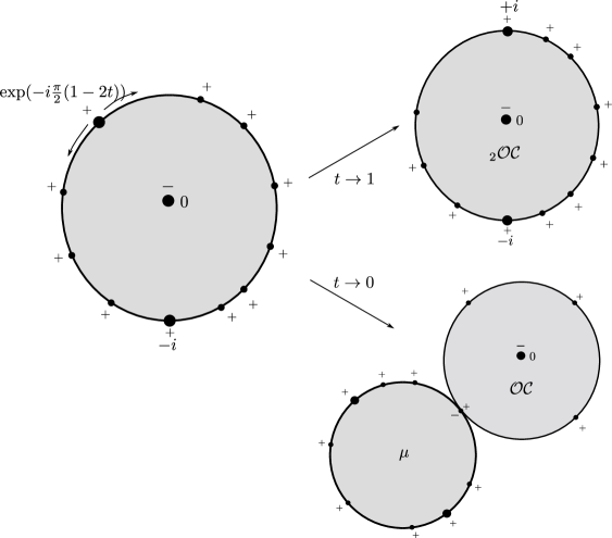
Figure 8. A schematic of $\mathcal{S}^{1}_{k,l}$ and its $t=0,1$ degenerations.

Definition 5.7.

The moduli space

(5.96) $$\mathcal{S}^{1,1}_{r,s}$$

is the space of discs with one interior positive puncture labeled $y_{in}$, one negative boundary puncture $z_{out}$, and $r+s+1$ positive boundary punctures, labeled in clockwise order from $z_{out}$ as $z_{1},\ldots,z_{r},z_{fixed},z_{1}^{\prime},\ldots,z_{s}^{\prime}$, subject to the following constraint:

(5.97) $$\begin{split}\textrm{up to automorphism, }&z_{out},\ z_{fixed},\ \textrm{and }y_{in}\ \textrm{lie at }-i,\ e^{i(-\pi/2+\pi\cdot t)}\ \textrm{and }0\textrm{ respectively},\\ &\textrm{for\ some\ }t\in(0,1).\end{split}$$

The space $\mathcal{S}^{1,1}_{r,s}$ again fibers over the open interval $(0,1)$, by the value of $t$ above. Compactifying, we see that the codimension 1 boundary strata of the space $\overline{\mathcal{S}}^{1,1}_{r,s}$ submerses over $[0,1]$ and is covered by the images of the natural inclusions of the following products (some corresponding to the limits $t=0,1$ and some occurring over the entire interval):

(5.98) $$\overline{\mathcal{R}}^{1,1}_{s-s^{\prime}-s^{\prime\prime}+1}\times_{r+2+s^{\prime}}\overline{\mathcal{R}}^{r+2+s^{\prime}+s^{\prime\prime}} \textrm{ }(t=0)$$

(5.99) $$\overline{\mathcal{R}}^{1,1}_{r,s} \textrm{ }(t=1)$$

(5.100) $$\overline{\mathcal{R}}^{r^{\prime}}\times_{n+1}\overline{\mathcal{S}}^{1,1}_{r-r^{\prime}+1,s} \ \ \ 0\leq n<r-r^{\prime}+1$$

(5.101) $$\overline{\mathcal{R}}^{s^{\prime}}\times_{(m+1)^{\prime}}\overline{\mathcal{S}}^{1,1}_{r,s-s^{\prime}+1} \ \ \ 0\leq m<s-s^{\prime}+1$$

(5.102) $$\overline{\mathcal{R}}^{r^{\prime}+s^{\prime}+1}\times_{0}\overline{\mathcal{S}}^{1,1}_{r-r^{\prime},s-s^{\prime}}$$

(5.103) $$\overline{\mathcal{S}}^{1,1}_{r-a^{\prime},s-b^{\prime}}\times_{a^{\prime}+1}\overline{\mathcal{R}}^{a^{\prime}+b^{\prime}+1}$$

Using sign twisting datum

(5.104) $$\vec{t}_{{}_{2}\mathcal{CO}\rightarrow\mathcal{CO},r,s}=(-1,0,\ldots,r-1,r+1,r+2,\ldots,r+s+1),$$

the associated operation

(5.105) $$\mathcal{G}:=\bigoplus_{r,s}(-1)^{\vec{t}_{{}_{2}\mathcal{CO}\rightarrow\mathcal{CO},r,s}}\mathbf{F}_{\overline{\mathcal{S}}^{1,1}_{r,s}}:CH^{*}(M)\longrightarrow{{}_{2}}\mathrm{CC}^{*}(\mathcal{W},\mathcal{W})$$

has degree $-1$. By analyzing the boundary of the 1-dimensional Floer moduli spaces associated to $\mathcal{S}^{1,1}_{r,s}$ coming from (5.87)-(5.92) and strip-breaking, and verifying signs (Appendix B), we see that

(5.106) $$\mathcal{G}\circ d_{CH}\pm d_{{{}_{2}}\mathrm{CC}^{*}}\circ\mathcal{G}=\mathbf{\Psi}\circ\mathcal{CO}-{{}_{2}}\mathcal{CO},$$

verifying the second homotopy commutative diagram.

6. Unstable operations

Some of the operations we would like to consider are parametrized not by underlying moduli spaces but instead a single surface.

6.1. Strips

Let $\Sigma_{1}$ denote a disc with two boundary punctures removed, thought of as a strip $(\infty,\infty)\times[0,1]$. We have already defined a Floer-theoretic operation using $\Sigma_{1}$, namely the differential $\mu^{1}$. Let us recast this operation in terms of Floer data.

Definition 6.1.

A Floer datum for $\Sigma_{1}$ can be thought of a Floer datum in the sense of Definition 4.11 with the following additional constraints:

• The strip-like ends $\epsilon_{+}$ and $\epsilon_{-}$ are given by inclusion of the positive and negative semi-infinite strips respectively.

• The incoming and outgoing weights are both equal to a single number $w$.

• the one-form $\alpha$ is $w\cdot dt$ everywhere, as is the rescaling map $a_{S}$.

• the Hamiltonian $H_{\Sigma_{1}}$ is equal everywhere to $\frac{H\circ\psi^{w}}{w^{2}}$

• the almost complex structure $J_{\Sigma_{1}}$ is equal everywhere to $(\psi^{w})^{*}J_{t}$.

Remark 6.1.

Upon fixing $H$ and $J_{t}$, the Floer datum above only depends on $w$. Moreover, the data defined by any two different weights $w$ and $w^{\prime}$ are conformally equivalent.

Fix the Floer datum for $\Sigma_{1}$ with $w=1$. This induces, for Lagrangians $L_{0},L_{1}\in\mathrm{ob\ }\mathcal{W}$, and chords $x_{0},x_{1}\in\chi(L_{0},L_{1})$, a space of maps

$$\Sigma_{1}(x_{0};x_{1})$$

satisfying the usual asymptotic and boundary conditions, and solving the relevant version of Floer’s equation for the Floer datum. Instead of dividing by ${\mathbb{R}}$-translation, we can also consider the operation induced by the space $\Sigma_{1}(x_{0};x_{1})$ itself, which has dimension

$$\deg(x_{0})-\deg(x_{1})$$

We get a map

(6.1) $$I:CW^{*}(L_{0},L_{1})\longrightarrow CW^{*}(L_{0},L_{1})$$

defined by

(6.2) $$I([x_{0}]):=\sum_{x_{1}:\deg(x_{1})=\deg(x_{0})}\sum_{u\in\Sigma_{1}(x_{0};x_{1})}(-1)^{\deg(x_{0})}(\Sigma_{1})_{u}([x_{0}])$$

where $(\Sigma_{1})_{u}:o_{x_{0}}\rightarrow o_{x_{1}}$ is the induced map on orientation lines (using Lemma B.1).

Proposition 6.1.

$I$ is the identity map.

Proof.

If $u$ is any non-constant strip mapping into $M$, composing with the ${\mathbb{R}}$ action on $\Sigma_{1}$ gives other maps into $M$ solving the same equation by ${\mathbb{R}}$-invariance of our Floer data; hence $u$ is not rigid. Therefore, dimension 0 strips must all be constant, concluding the proof. ∎

6.2. The unit

Let $\Sigma_{0}$ denote a once-punctured disc thought of as the upper half plane ${\mathbb{H}}\subset{\mathbb{C}}$ with puncture at $\infty$, thought of as a negative puncture.

Definition 6.2.

A Floer datum for $\Sigma_{0}$ is a Floer datum in the sense of Definition 4.11. Concretely, this consists of

• A strip-like end $\epsilon:(-\infty,0]\times[0,1]\rightarrow\Sigma_{0}$ around the puncture

• A choice of weight $w\in[1,\infty)$

• A rescaling map $a_{\Sigma_{0}}:\Sigma_{0}\rightarrow[1,+\infty)$ equal to $w$ on the strip-like end

• Hamiltonian perturbation: A map $H_{\Sigma_{0}}:\Sigma_{0}\rightarrow\mathcal{H}(M)$ such that $\epsilon^{*}H_{\Sigma_{0}}=\frac{H\circ\psi^{w}}{w^{2}}$.

• basic 1-form: a sub-closed 1-form $\alpha_{\Sigma_{0}}$, whose restriction to $\partial\Sigma_{0}$ vanishes, such that $\epsilon^{*}\alpha_{\Sigma_{0}}=w\cdot dt$.

• Almost complex structure: A map $J_{\Sigma_{0}}:\Sigma_{0}\rightarrow\mathcal{J}(M)$ such that $J_{\Sigma_{0}}\in\mathcal{J}_{a_{\Sigma_{0}}}$ and $\epsilon^{*}J_{\Sigma_{0}}=(\psi^{w})^{*}J_{t}$.

Remark 6.2.

Note by Stokes’ theorem that in the definition above, the one form $\alpha_{\Sigma_{0}}$ cannot be closed everywhere, i.e. there are points with $d\alpha_{\Sigma_{0}}<0$.

Remark 6.3.

Up to conformal equivalence, it suffices to take a Floer datum for $\Sigma_{0}$ with weight $w=1$.

Let $L$ be an object of $\mathcal{W}$, and consider a chord $x_{0}\in\chi(L,L)$. Fixing a Floer datum for $\Sigma_{0}$, write

(6.3) $$\Sigma_{0}(x_{0};)$$

for the space of maps $u:\Sigma_{0}\rightarrow E$ satisfying boundary and asymptotic conditions

(6.4) $$\begin{cases}u(z)\in\psi^{a_{S}(z)}L&z\in\partial\Sigma_{0}\\ \lim_{s\rightarrow-\infty}u\circ\epsilon(s,\cdot)=x\end{cases}$$

and differential equation

(6.5) $$(du-X_{\Sigma_{0}}\otimes\alpha_{\Sigma_{0}})^{0,1}=0$$

with respect to $J_{\Sigma_{0}}$.

Lemma 6.1.

The space of maps $\Sigma_{0}(x_{0};)$ is compact and forms a manifold of dimension $\deg(x_{0})$.

Thus, we can define the element $e_{L}\in CW^{*}(L,L)$ to be the sum

(6.6) $$e_{L}:=\sum_{\deg(x_{0})=0}\sum_{u\in\Sigma_{0}(x_{0};)}(\Sigma_{0})_{u}(1)$$

where $(\Sigma_{0})_{u}:{\mathbb{R}}\rightarrow o_{x_{0}}$ is the induced map on orientation lines (using Lemma B.1)

Proposition 6.2.

The resulting elements $e_{L_{i}}\in CW^{*}(L_{i},L_{i})$ give the identity element on homology.

Proof.

This is a classical result, but we briefly sketch a proof for completeness; see e.g. [Ritter:2010nx] for more details. One first checks via analyzing the boundary of the one dimensional moduli space of $\Sigma_{0}(x_{0};)$ that $d(e_{L})=0$, so $e_{L}$ descends to homology. Then, one needs to check that, up to sign

(6.7) $$\mu^{2}([x],[e_{L_{i}}]) =[x]$$

(6.8) $$\mu^{2}([e_{L_{i}}],[x]) =[x],$$

where the brackets denote homology classes. Since the arguments to establish (6.7) and (6.8) are identical, it suffices to construct a geometric chain homotopy between the maps

(6.9) $$\mu^{2}(\cdot,e_{L_{i}})$$

and

(6.10) $$I(\cdot)$$

where $I$ is as in (6.1), which can be described as follows. Let $\Sigma_{2}$ be a disc with two incoming boundary marked points $x_{1}$, $x_{2}$, and one outgoing point $x_{out}$, with $x_{1}$ marked as “forgotten” (see Section 10 for how to do this). Fix a strip-like end around $x_{1}$ and consider a one parameter family of Floer data on $\Sigma_{2}$ with $x_{2}$ and $x_{out}$ removed, over the interval $[0,1)_{t}$, such that

• at $t=0$, the Floer data agrees with the translation-invariant one on the $\Sigma_{1}$ arising by forgetting $x_{1}$,

• for general $t$, the Floer data is modeled on the connect sum of the Floer data for $\mu_{2}$ with the Floer data for $e_{L_{i}}$ over the strip-like ends at the output of $\Sigma_{0}$ with the one around $x_{1}$, with connect sum length approaching $\infty$ as $t\rightarrow 1$.

Compactifying and looking at the associated Floer operation, one obtains a chain homotopy between the degenerate curve corresponding to $\mu(\cdot,e_{L_{i}})$ and the operation $I(\cdot)$. Finally, one performs a sign verification analogous to those in Appendix B. ∎

7. Operations from glued pairs of discs

In this section, we define a broad class of abstract moduli spaces and their associated Floer theoretic operations, corresponding to a pair of discs glued together along some boundary components. This class will arise when defining operations in the product $M^{-}\times M$, and in setting up the theory of quilts.

7.1. Connect sums

We give a short aside on the notation we use for connect sums. Recall first the notion of a boundary connect sum between two Riemann surfaces with boundary, a notion already implicit in our constructions of Deligne-Mumford compactifications of moduli spaces.

Definition 7.1.

Let $\Sigma_{1},\Sigma_{2}$ be two Riemann surfaces with boundary, with marked points $z_{1}\in\partial\Sigma_{1}$, $z_{2}\in\partial\Sigma_{2}$ removed. Let $\epsilon_{1}:Z_{+}\rightarrow\Sigma_{1}$ be a positive strip-like end for $z_{1}$ and $\epsilon_{2}:Z_{-}:\rightarrow\Sigma_{2}$ a negative strip-like end for $z_{2}$ and let $\lambda=\frac{\log\rho}{1+\log\rho}\in(0,1)$ (correspondingly $\rho\in[1,\infty)$). The $\lambda$-connect sum

(7.1) $$\Sigma_{1}\#_{(\epsilon_{1},z_{1}),(\epsilon_{2},z_{2})}^{\lambda}\Sigma_{2}$$

is

(7.2) $$\left(\Sigma_{1}-\epsilon_{1}([\rho,\infty)\times[0,1])\right)\cup_{\varphi_{\rho}}\left(\Sigma_{2}-\epsilon_{2}((-\infty,-\rho]\times[0,1])\right)$$

where

(7.3) $$\varphi_{\rho}:\epsilon_{1}((0,\rho)\times[0,1])\rightarrow\epsilon_{2}((-\rho,0)\times[0,1]).$$

is the composition

(7.4) $$\epsilon_{1}((0,\rho)\times[0,1])\stackrel{{\scriptstyle\epsilon_{1}^{-1}}}{{\rightarrow}}(0,\rho)\times[0,1]\stackrel{{\scriptstyle(\cdot-\rho,id)}}{{\rightarrow}}(-\rho,0)\times[0,1]\stackrel{{\scriptstyle\epsilon_{2}}}{{\rightarrow}}\epsilon_{2}((-\rho,0)\times[0,1]).$$

We will often write $\Sigma_{1}\#^{\lambda}_{z_{1},z_{2}}\Sigma_{2}$ when the choice of strip-like ends is implicit.

Definition 7.2.

In the notation of above, the associated thin part of a $\lambda$-connect sum $\Sigma_{1}\#^{\lambda}_{z_{1},z_{2}}\Sigma_{2}$ is the finite strip parametrization

(7.5) $$\epsilon_{1}:[0,\rho]\times[0,1]\rightarrow\Sigma_{1}\#^{\lambda}_{z_{1},z_{2}}\Sigma_{2}.$$

The associated thick parts of this connect sum are the regions $\Sigma_{1}-\epsilon_{1}([0,\infty)\times[0,1])$, $\Sigma_{2}-\epsilon_{2}([-\infty,0]\times[0,1])$ respectively, thought of as living in the connect sum.

The notion of $\lambda$ connect sum extends continuously to the nodal case $\lambda=1$.

7.2. Pairs of discs

Definition 7.3.

The moduli space of pairs of discs with $(k,l)$ marked points, denoted

(7.6) $$\mathcal{R}_{k,l}$$

is the moduli space of pairs of discs with $k$ and $l$ positive marked points and one negative marked point each in the same position, modulo simultaneous automorphisms.

Remark 7.1.

This definition is not identical to the product of associahedra $\mathcal{R}^{k}\times\mathcal{R}^{l}$. The latter space is a further quotient of the former space by automorphisms of the right or left disc, at least when both $k$ and $l$ are in the stable range. Operations at the level of the moduli space $\mathcal{R}_{k,l}$ will arise via quilted strips and homotopy units.

Remark 7.2.

To construct moduli spaces, we require a pair of discs with $(k,l)$ marked points to be stable: one of $k$ or $l$ must be at least two.

The Stasheff associahedron embeds in $\mathcal{R}_{k,l}$ in several ways. There is the diagonal embedding

(7.7) $$\mathcal{R}^{d}\stackrel{{\scriptstyle\Delta_{d}}}{{\lhook\joinrel\relbar\joinrel\rightarrow}}\mathcal{R}_{d,d}.$$

which is self-explanatory. When $l=1$ and $k\geq 2$, there is a one-sided embedding

(7.8) $$\mathcal{R}^{k}\stackrel{{\scriptstyle\mathcal{I}_{k}}}{{\lhook\joinrel\relbar\joinrel\rightarrow}}\mathcal{R}_{k,1},$$

where $\mathcal{I}_{k}=(id,For_{k-1})$ is the pair of maps corresponding to inclusion and forgetting the first $k-1$ boundary marked points respectively. Since the right factor in the image has only one incoming marked point, we call $\mathcal{I}_{k}$ the right semi-stable embedding. Similarly when $k=1$ and $l\geq 2$, forgetting $l-1$ marked points and inclusion gives us the left semi-stable embedding

(7.9) $$\mathcal{R}^{k}\stackrel{{\scriptstyle\mathcal{J}_{k}}}{{\lhook\joinrel\relbar\joinrel\rightarrow}}\mathcal{R}_{1,k}.$$

When $l=0$ or $k=0$, there are also equivalences

(7.10) $$\begin{split}\mathcal{R}^{k}&\stackrel{{\scriptstyle\sim}}{{\lhook\joinrel\relbar\joinrel\rightarrow}}\mathcal{R}_{k,0}\\ \mathcal{R}^{l}&\stackrel{{\scriptstyle\sim}}{{\lhook\joinrel\relbar\joinrel\rightarrow}}\mathcal{R}_{0,l},\end{split}$$

which we call the right and left ghost embeddings respectively, corresponding to the fact that the right or left component of $\mathcal{R}_{k,l}$ is a ghost disc. In fact, we will never consider operations with either $k$ or $l$ equal to zero, but these equivalences help us explain appearances of ordinary associahedra in the compactification $\overline{\mathcal{R}}_{k,l}$. Henceforth, let us restrict to $k,l\geq 1$ and one of $k,l\geq 2$.

The open moduli space $\mathcal{R}_{k,l}$ admits a stratification by coincident points between factors, which we will find useful to explicitly describe.

Definition 7.4.

A $(k,l)$-point identification $\mathfrak{P}$ is a sequence of tuples

(7.11) $$\{(i_{1},j_{1}),\ldots,(i_{s},j_{s})\}\subset\{1,\ldots,k\}\times\{1,\ldots,l\}$$

which are strictly increasing, i.e.

(7.12) $$\begin{split}i_{r}&<i_{r+1}\\ j_{r}&<j_{r+1}\end{split}$$

The number of coincidences of $\mathfrak{P}$ is the size $|\mathfrak{P}|$.

Definition 7.5.

Take a representative $(S_{1},S_{2})$ of a point in $\mathcal{R}_{k,l}$. A boundary input marked point $p_{1}$ on $S_{1}$ is said to coincide with a boundary marked input marked point $p_{2}$ on $S_{2}$ if they are at the same position when $S_{1}$ is superimposed upon $S_{2}$. This notion is independent of the representative $(S_{1},S_{2})$, as we act by simultaneous automorphism.

Definition 7.6.

The space of $\mathfrak{P}$-coincident pairs of discs with $(k,l)$ marked points

(7.13) $${}_{\mathfrak{P}}\mathcal{R}_{k,l}$$

is the subspace of $\mathcal{R}_{k,l}$ where pairs of input marked points on each factor specified by $\mathfrak{P}$ are required to coincide, and no other input marked points are allowed to coincide. Here the indices in $\mathfrak{P}$ coincide with the counter-clockwise ordering of input marked points on each factor.

Example 7.1.

When $\mathfrak{P}=\emptyset$, ${}_{\mathfrak{P}}\mathcal{R}_{k,l}$ is the space of pairs of discs where none of the inputs are allowed to coincide. This is a disconnected space, with connected components determined by the relative ordering of the $k$ inputs on the first disc with the $l$ inputs on the second disc. The number of connected components is exactly the number of $(k,l)$ shuffles, i.e. re-orderings of the sequence

(7.14) $$\{a_{1},\ldots,a_{k},b_{1},\ldots,b_{l}\}$$

that preserve relative ordering of the $a_{i}$, and the relative ordering of the $b_{j}$. Given a fixed $(k,l)$ shuffle, the subspace of pairs of discs with appropriate relatively ordered inputs is a copy of the $k+l$ associahedron $\mathcal{R}^{k+l}$. Equivalently, there is one copy of $\mathcal{R}^{k+l}$ for each $(k,l)$ two-coloring of the combined set of points, that is a collection of subsets

(7.15) $$I,J\subset[k+l],\ |I|=k,\ |J|=l,\ I\cup J=[k+l].$$

where $[k+l]:=\{1,\ldots,k+l\}$.

Example 7.2.

When $k=l$ and $|\mathfrak{P}|=k$ is maximal, the associated space ${}_{\mathfrak{P}}\mathcal{R}_{k,l}$ is just the diagonal associahedron. $\Delta_{k}(\mathcal{R}^{k})$.

We often group these spaces ${}_{\mathfrak{P}}\mathcal{R}_{k,l}$ by the number of coincident points.

Definition 7.7.

The space of pairs of discs with $(k,l)$ marked points and $i$ coincident points is defined to be

(7.16) $${}_{i}\mathcal{R}_{k,l}:=\coprod_{|\mathfrak{P}|=i}{{}_{\mathfrak{P}}}\mathcal{R}_{k,l}.$$

The closure of a stratum ${}_{i}\mathcal{R}_{k,l}$ in $\mathcal{R}_{k,l}$ is $\coprod_{j\geq i}{{}_{i}}\mathcal{R}_{k,l}$. Moreover, each stratum ${}_{i}\mathcal{R}_{k,l}$ can be explicitly described as a union of associahedra.

Definition 7.8.

Fix disjoint subsets $I$,$J$,$K$ of $[d]=\{1,\ldots,d\}$ such that

(7.17) $$I\cup J\cup K=[d].$$

The space of $(I,J,K)$ tricolored discs with $d$ inputs

(7.18) $${}_{I,J,K}\mathcal{R}^{d}$$

is exactly the ordinary associahedron, with inputs labeled by the elements $\{L,R,LR\}$ according to whether they are in the set $I$,$J$,or $K$. The space of $(i,j,k)$ tricolored discs with $d$ inputs, where $i+j+k=d$, is the disjoint union over all possible tricolorings of cardinality $i,j,k$:

(7.19) $${{}_{i,j,k}}\mathcal{R}^{d}:=\coprod_{|I|=i,|J|=j,|K|=k}{{}_{I,J,K}}\mathcal{R}^{d}.$$

There is a canonical identification

(7.20) $${}_{i}\mathcal{R}_{k,l}\simeq{{}_{k-i,l-i,i}}\mathcal{R}^{k+l-i}$$

given as follows: To a pair of discs $(S_{1},S_{2})$ with $i$ coincidences, consider the overlay (superimposition) of $S_{1}$ and $S_{2}$ along with their marked points. This is a disc with $k+l-i$ input marked points and one output. Color a marked point $L$ if the marked point came only from $S_{1}$, $R$ if the marked point came only from $S_{2}$, and $LR$ if the marked point came from both factors. Similarly, given a tricolored disc, one can reconstruct a pair of discs with $i$ coincidences by reversing the above procedure.

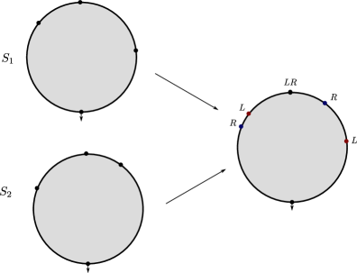
Figure 9. An example of the correspondence between pairs of discs and tricolored discs.

The disjoint union of spaces

(7.21) $$\coprod_{i}{{}_{k-i,l-i,i}}\mathcal{R}^{k+l-i}$$

is set theoretically the same as $\mathcal{R}_{k,l}$, but has forgotten some of the topology. Namely, points colored $L$ and $R$ are not allowed to coincide, and coincident points (those colored $LR$) are not allowed to separate arbitrarily.

We now construct a model for the Deligne-Mumford compactification

(7.22) $$\overline{\mathcal{R}}_{k,l}.$$

The main idea in our construction is to recover this compactification from the Deligne-Mumford compactifications of the spaces ${}_{k-i,l-i,i}\overline{\mathcal{R}}^{k+l-i}$ by reconstructing the topology with which points colored $L$ and $R$ are allowed to coincide, and points colored $LR$ are allowed to separate. Note that the compactification of tricolored spaces

(7.23) $${}_{I,J,K}\overline{\mathcal{R}}^{d}$$

is exactly the usual Deligne-Mumford compactification, where boundary marked points on components of nodal discs are colored in a manner induced by the gluing charts (5.3). Internal positive marked points are colored in the following induced fashion: If the subtree of nodal discs lying above a given positive marked point is a tree of discs with all $L$ or all $R$ labels, then color this marked point $L$ or $R$ respectively. If the subtree contains two out of the three colors ($R$, $L$, $RL$) then color the input $LR$.

Let

(7.24) $$D_{LR}^{+1}$$

be a representative of the one-point moduli space ${}_{\{1\},\{2\},\emptyset}\mathcal{R}^{2}$, i.e. a disc with inputs labeled $L,R$ in clockwise order. Similarly, let

(7.25) $$D_{LR}^{-1}$$

be a representative of ${}_{\{2\},\{1\},\emptyset}\mathcal{R}^{2}$, i.e. a disc with inputs labeled $R,L$ in clockwise order. Fix a choice of strip-like ends on $D_{LR}^{\pm 1}$, and let $z_{LR}$ denote the output of each of these discs. Also, suppose we have fixed a universal and consistent choice of strip like ends on the various ${}_{k-i,l-i,i}\overline{\mathcal{R}}^{k+l-i}$.

Now, take a (potentially nodal) representative $S$ of a point of ${}_{k-i,l-i,i}\overline{\mathcal{R}}^{k+l-i}$. Let

(7.26) $$\vec{p}=p_{j_{1}},\ldots p_{j_{s}},\ s\leq i$$

be a subset of the points colored $LR$, and $\epsilon_{j_{1}},\ldots,\epsilon_{j_{s}}$ the associated strip-like ends. Given a vector

(7.27) $$\vec{v}=(v_{1},\ldots,v_{j_{s}})\in[(-\epsilon,\epsilon)^{*}]^{i},$$

where the $*$ means none of the $v_{r}$ are allowed to be zero, define an element

(7.28) $$\mathbf{\Pi}^{\vec{p}}_{\vec{v}}(S)\in{{}_{k-i+s,l-i+s,i-s}}\overline{\mathcal{R}}^{k+l-i+s}$$

by the iterated connect sum

(7.29) $$\mathbf{\Pi}_{\vec{v}}^{\vec{p}}(S):=S\#_{p_{j_{1}},z_{LR}}^{1-|v_{1}|}D^{\mathrm{sign}(v_{1})}_{LR}\#\cdots\#_{p_{j_{k}},z_{LR}}^{1-|v_{j}|}D^{\mathrm{sign}(v_{j})}_{LR}.$$

Here $\#^{1-|v_{r}|}$ is the operation of connect sum with gluing parameter $1-|v_{r}|$ in the notation of Section 7.1, which as $|v_{R}|$ approaches zero is very close to nodal. Also, $\mathrm{sign}(v_{r})$ is $+1$ if $v_{r}$ is positive and $-1$ if $v_{r}$ is negative. In other words, at input point $p_{j_{r}}$ on $S$, we are taking a connect sum with the disc $D^{\mathrm{sign}(v_{r})}_{LR}$ at the point $z_{LR}$, i.e. gluing in two points labeled $L$ and $R$ in clockwise or counterclockwise order depending on the sign of $v_{r}$.

Example 7.3.

It is useful before proceeding to describe the map $\Pi^{\vec{p}}_{\vec{v}}(S)$ in a simple example. Suppose we are in ${}_{1,1,1}\mathcal{R}^{3}$, the moduli space of discs with three inputs, one with each color. Pick a non-nodal representative of an element of this space, without loss of generality one in which the points are colored $L$, $LR$ and $R$ in clockwise order from the output. Let $p_{2}$ be the point colored $LR$ with associated vector $\vec{v}=(v)$, and let us examine the representative of $\Pi_{(v)}^{p_{2}}(S)$ for different values of $v\in(-\epsilon,0)\cup(0,\epsilon)$. For $v$ positive, $\Pi^{p_{2}}_{(v)}(S)$ corresponds to resolving the $LR$ point by two points, one labeled $L$ and one labeled $R$, with the $L$ point to the left of the $R$ point, which lives in ${}_{\{1,2\},\{3,4\},\emptyset}\mathcal{R}^{4}$. For $v$ negative, we $\Pi^{p_{2}}_{(v)}(S)$ resolves the $LR$ point in the opposite direction, giving an element of a different associahedron ${}_{\{1,3\},\{2,4\},\emptyset}\mathcal{R}^{4}$. As $v$ approaches zero from either direction, the newly created $L$ and $R$ points come together and bubble off, giving a nodal element in each of these respective associahedra $\Pi^{p_{2}}_{(0+)}(S)$ and $\Pi^{p_{2}}_{(0-)}(S)$ with bubble component a $D_{LR}^{+1}$ or $D_{LR}^{-1}$ respectively. To partially recover the topology of $\mathcal{R}_{2,2}$, we would like to identify the points $\Pi^{p_{2}}_{0-}(S)$ and $\Pi^{p_{2}}_{0+}(S)$, in a manner preserving the manifold structure near the identification. See Figure 10.

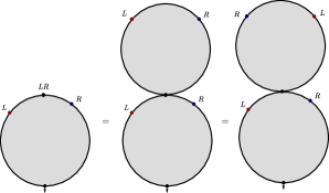
Figure 10. The strata we would like to identify.

The above example illustrates the following properties: $\Pi_{\vec{v}}$ varies smoothly in $S$ and the parameters $\vec{v}\in[(-\epsilon,\epsilon)^{*}]^{i}$, and there are well defined, but different, nodal limits of the curve $\Pi_{\vec{v}}(S)$ as components $v_{r}$ approach 0 from the left or right, corresponding to gluing on a nodal $D_{LR}^{\pm 1}$ respectively at input $p_{j_{r}}$. Indicate these different limits by values $0_{+}$ and $0_{-}$ respectively. Then $\Pi_{\vec{v}}(S)$ extends to a map

(7.30) $$\bar{\Pi}_{\vec{v}}$$

defined over domain

(7.31) $$\vec{v}\in\left[(-\epsilon,0_{-}]\cup[0_{+},\epsilon)\right]^{i}.$$

Define

(7.32) $${}_{k-i,l-i,i}(\overline{\mathcal{R}}^{k+l-i})^{*}$$

to be the locus of the compactifications ${}_{I,J,K}\overline{\mathcal{R}}^{k+l-i}$ with $|I|=k-i$, $|J|=l-i$, $|K|=i$ where there are no leaf bubbles with one $L$ and one $R$. Put another way, remove the images of $\bar{\Pi}^{\vec{p}}_{(\cdots,0_{+},\cdots)}$, $\bar{\Pi}^{\vec{p}}_{(\cdots,0_{-},\cdots)}$ for all relevant domains of definition of $\Pi$. Now, define the manifold structure on $\overline{\mathcal{R}}_{k,l}$ as follows. To simplify notation, denote

(7.33) $${\mathbb{I}}_{\epsilon}:=(-\epsilon,\epsilon).$$

Charts consist of

(7.34) $$\mathcal{U}\times{\mathbb{I}}_{\epsilon}^{i},\ \mathcal{U}\subset{{}_{k-i,l-i,i}}(\overline{\mathcal{R}}^{k+l-i})^{*}.$$

where $\epsilon$ may depend on $\mathcal{U}$.

For every such $\mathcal{U}$ above take any subset of indices $\vec{j}=\{j_{1},\ldots,j_{s}\}$ of the $i$ points colored $LR$, indexed for now from $1$ to $i$. Let $\vec{p}=\{p_{j_{1}},\ldots,p_{j_{s}}\}$ be the associated points. Given any such subset $\vec{j}$ of $\{1,\ldots,i\}$, define

(7.35) $$\mathcal{P}_{\vec{j}}:{\mathbb{I}}_{\epsilon}^{i}\longrightarrow{\mathbb{I}}_{\epsilon}^{|\vec{j}|}$$

to be the projection onto the coordinates with indices in $\vec{j}$ and

(7.36) $$\mathcal{P}_{\vec{j}^{c}}:{\mathbb{I}}_{\epsilon}^{i}\longrightarrow{\mathbb{I}}_{\epsilon}^{i-|\vec{j}|}$$

to be the projection onto the complementary coordinates.

Then shrinking $\mathcal{U}$ and $\epsilon$ if necessary, perform a smooth identification of the restriction of the basic chart (7.34), where the coordinates for indices in $\vec{j}$ are all non-zero

(7.37) $$\mathcal{U}\times{\mathbb{I}}_{\epsilon}^{i}|_{\mathcal{P}_{\vec{j}}^{-1}(({\mathbb{I}}_{\epsilon}^{*})^{|\vec{j}|})}$$

onto its image under the smooth map

(7.38) $$(S,\vec{v})\longmapsto(\Pi^{\vec{p}}_{\mathcal{P}_{\vec{j}}(\vec{v})}(S),\mathcal{P}_{\vec{j}^{c}}(\vec{v})).$$

All such identifications are manifestly compatible with each other, and along with the identifications of charts within each ${}_{k-i,l-i,i}\mathcal{R}^{k+l-i}$, give $\overline{\mathcal{R}}_{k,l}$ the structure of a smooth manifold with corners of dimension $k+l-2$. The result is moreover compact, as topologically it is the quotient of the compact space ${}_{k,l,0}\overline{\mathcal{R}}^{k+l}$ by identifications between otherwise identical nodal surfaces containing $D_{LR}^{\pm}$ components.

Example 7.4.

Let us examine the resulting manifold structure on $\overline{\mathcal{R}}_{2,2}$, in a neighborhood of the one point coincidence discussed in Example 7.3. Consider once more the element $q$ of ${{}_{1,1,1}}\mathcal{R}^{3}$ we discussed there, which is represented by some disc with inputs colored $L$, $LR$, and $R$ in clockwise order. Then, in a neighborhood $U_{q}$ of $q$, we have a chart

(7.39) $$U_{q}\times(-\epsilon,\epsilon)$$

for some small value of $\epsilon$. There are two distinguished smooth identifications of subsets of (7.39). In the first, one resolves the $LR$ point $p_{2}$ by an $L$ followed by $R$

(7.40) $$\begin{split}U_{q}\times(0,\epsilon)&\longrightarrow{{}_{2,2,0}}\mathcal{R}^{4}\\ (S,v)&\longmapsto\Pi^{p_{2}}_{(v)}(S):=S\#_{p_{2}}^{1-v}D_{LR}^{+1}\end{split}$$

and in the second, one resolves $p_{2}$ by an $R$ followed by an $L$

(7.41) $$\begin{split}U_{q}\times(-\epsilon,0)&\longrightarrow{{}_{2,2,0}}\mathcal{R}^{4}\\ (S,v)&\longmapsto\Pi^{p_{2}}_{(v)}(S):=S\#_{p_{2}}^{1-(-v)}D_{LR}^{-1}.\end{split}$$

These identifications, along with the existing manifold structure on $({{}_{2,2,0}}\overline{\mathcal{R}}^{4})^{*}$ determine the manifold structure in a neighborhood of $p_{2}$. See Figure 11 for an illustration of the manifold structure near $p_{2}$.

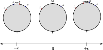
Figure 11. The manifold structure near a coincident point on $\mathcal{R}_{2,2}$.

This definition of the compactification $\overline{\mathcal{R}}_{k,l}$ remembers the structure of the left and right components. Namely, a (potentially nodal) element $S$ in $\overline{\mathcal{R}}_{k,l}$ can be thought of as an element of ${}_{k-i,l-i,i}\overline{\mathcal{R}}^{k+l-i}$ for some $i$, with no $D_{LR}^{\pm}$ leaf bubbles. Define the associated unreduced left disc $\tilde{S}_{1}$ to be obtained from $S$ by deleting all points colored $R$, and forgetting the $L$, $LR$ colorings. Similarly, define the associated unreduced right disc $\tilde{S}_{2}$ to be obtained by deleting all points colored $L$ and forgetting the $R$, $RL$ colorings. The associated reduced discs $(S_{1},S_{2})$ are given by stabilizing $\tilde{S}_{1}$ and $\tilde{S}_{2}$, and there are well defined inputs on these stabilizations corresponding to the inputs colored $(L,LR)$ and $(LR,R)$ on $S$ respectively.

In this way, we obtain a projection map

(7.42) $$\pi_{reduce}:\overline{\mathcal{R}}_{k,l}\longrightarrow\bar{\mathcal{R}}^{k}\times\bar{\mathcal{R}}^{l}$$

Since the manifolds ${}_{k-i,l-i,i}\mathcal{R}^{k+l-i}$ are codimension $i$ in the space $\mathcal{R}_{k,l}$, we see that the codimension one boundary of the compactification $\overline{\mathcal{R}}_{k,l}$ is contained in the image of the codimension 1 boundary of the top stratum ${}_{k,l,0}\overline{\mathcal{R}}^{k+l}$. The chart identifications (7.38) show that points where an $L$ and $R$ would have bubbled off in codimension 1 now cease to be boundary points; thus any codimension 1 bubble must contain at least two $L/LR$ points or two $R/LR$ points.

The result of this discussion is as follows: we see that the codimension one boundary of the Deligne-Mumford compactification (7.22) is covered by the images of the natural inclusions of the following products:

(7.43) $$\overline{\mathcal{R}}_{k^{\prime},l^{\prime}} \times{{}_{1}}\overline{\mathcal{R}}_{k-k^{\prime}+1,l-l^{\prime}+1},\ k^{\prime},l^{\prime},k-k^{\prime}+1,l-l^{\prime}+1\geq 2$$

(7.44) $$\overline{\mathcal{R}}_{k^{\prime},1} \times{{}_{1}}\overline{\mathcal{R}}_{k-k^{\prime}+1,l},\ k^{\prime},k-k^{\prime}+1,\geq 2$$

(7.45) $$\overline{\mathcal{R}}_{1,l^{\prime}} \times{{}_{1}}\overline{\mathcal{R}}_{k,l-l^{\prime}+1},\ l^{\prime},l-l^{\prime}+1\geq 2$$

(7.46) $$\overline{\mathcal{R}}_{k^{\prime},0} \times\overline{\mathcal{R}}_{k-k^{\prime}+1,l},\ k^{\prime},k-k^{\prime}+1\geq 2$$

(7.47) $$\overline{\mathcal{R}}_{0,l^{\prime}} \times\overline{\mathcal{R}}_{k,l-l^{\prime}+1},\ l^{\prime},l-l^{\prime}+1\geq 2$$

The appearance of 1-coincident spaces ${{}_{1}}\mathcal{R}_{k-k^{\prime}+1,l-l^{\prime}+1}$ in (7.43)-(7.45) has a simple explanation. For simultaneous bubbling of $L$ and $R$’s to occur, the bubble point must be coincident, i.e. colored $LR$.

Strictly speaking, the compactification we have described is somewhat larger than we would ideally like; the strata of most interest to us are (7.46) and (7.47). However, we will be able to make arguments showing that operations coming from the other strata must all be zero.

Remark 7.3.

We could further reduce the compactification of $\mathcal{R}_{k,l}$ by collapsing strata whose subtrees are monochromatic $L$ or $R$ except for a single off-color point. The construction would make points colored $R$ point view entire subtrees colored $L$ as invisible and vice versa. Having made this construction, one can then check that the resulting operations we construct will not change. We have thus opted for a simpler construction at the expense of having a larger compactification.

7.3. Sequential point identifications

We study a particular classes of submanifolds of pairs of discs, and examine its compactifications carefully. This compactification is the one that will arise when defining quilts and Floer theoretic operations in the product.

Definition 7.9.

A point identification $\mathfrak{P}$ is said to be sequential if it is of the form

(7.48) $$\mathfrak{S}=\{(i_{1},j_{1}),(i_{1}+1,j_{1}+1),\ldots,(i_{1}+s,j_{1}+s)\}.$$

It is further said to be initial if $(i_{1},j_{1})=(1,1)$.

Definition 7.10.

A cyclic sequential point identification of type ($r,s$) is one of the form

(7.49) $$\mathfrak{S}=\{(1,1),(2,2),\ldots,(r,r),(k-s,l-s),(k-s+1,l-s+1),\ldots,(k,l)\}.$$

In other words, it is a sequential point identification where we need to take indices mod $(k,l)$.

Proposition 7.1.

Let $\mathfrak{P}$ be a $(k,l)$ initial sequential point identification of length $s$. Then the codimension-1 boundary of the compactification of $\mathfrak{P}$-identified pairs of discs

(7.50) $${}_{\mathfrak{P}}\overline{\mathcal{R}}_{k,l}$$

is covered by the natural inclusions of the following products:

(7.51) $${{}_{\mathfrak{P}_{max}}}\overline{\mathcal{R}}_{d,d} \times{{}_{\mathfrak{P}^{\prime}}}\overline{\mathcal{R}}_{k-d+1,l-d+1}$$

(7.52) $${{}_{\mathfrak{P}^{\prime}}}\overline{\mathcal{R}}_{k^{\prime},l^{\prime}} \times{{}_{\mathfrak{P}^{\prime\prime}}}\overline{\mathcal{R}}_{k-k^{\prime}+1,l-l^{\prime}+1}$$

(7.53) $$\overline{\mathcal{R}}_{k^{\prime},l^{\prime}} \times{{}_{\mathfrak{P}\cup(s,t)}}\overline{\mathcal{R}}_{k-k^{\prime}+1,l-l^{\prime}+1}$$

(7.54) $$\overline{\mathcal{R}}_{k^{\prime},1} \times{{}_{\mathfrak{P}\cup(s,t)}}\overline{\mathcal{R}}_{k-k^{\prime}+1,l}$$

(7.55) $$\overline{\mathcal{R}}_{1,l^{\prime}} \times{{}_{\mathfrak{P}\cup(s,t)}}\overline{\mathcal{R}}_{k,l-l^{\prime}+1}$$

(7.56) $$\overline{\mathcal{R}}_{0,l^{\prime}} \times{{}_{\mathfrak{P}}}\overline{\mathcal{R}}_{k,l-l^{\prime}+1}$$

(7.57) $$\overline{\mathcal{R}}_{k^{\prime},0} \times{{}_{\mathfrak{P}}}\overline{\mathcal{R}}_{k-k^{\prime}+1,l}.$$

Proof.

We will only say a few words about the Proposition. Note that under the point-coincidence stratification, the top stratum of the non-compactified space ${}_{\mathfrak{P}}\mathcal{R}_{k,l}$, in which there are no other coincidences, correspond to all tricolorings of discs with $k+l-i$ marked points with $LR$ colorings specified by $\mathfrak{P}$ and $L$, $R$ colorings arbitrary

(7.58) $${}_{\mathfrak{P}}\mathcal{R}_{k,l}=\coprod_{I\cup J\cup\mathfrak{P}=[k+l-i]}{{}_{I,J,\mathfrak{P}}}\mathcal{R}^{k+l-|\mathfrak{P}|}.$$

Thus, we can determine the codimension-one boundary of the compactification by looking at the boundary components of the compactifications ${}_{I,J,\mathfrak{P}}\overline{\mathcal{R}}_{k,l}$ which survive our chart maps (7.38).

The possible strata that arise fall into three different cases: bubbling occurs entirely within the coincident points (7.51), bubbling overlaps somewhat with the coincident points (7.52), and bubbling stays entirely away from the coincident points (7.53) - (7.57). Note once more that when $L$ and $R$ points simultaneously bubble, there is an additional coincident point created, hence the need to add various $(s,t)$ to the coincident set in (7.53)-(7.55). ∎

7.4. Gluing discs

We now make precise the notion of gluing pairs of discs along some identified boundary components, a construction that will arise from incorporating the diagonal Lagrangian $\Delta$ as an admissible Lagrangian in the product $M^{-}\times M$. We begin by discussing the combinatorial type of a boundary identifications of a pair of discs.

Definition 7.11.

A $(k,l)$ boundary identification is a subset $\mathfrak{S}$ of the set of pairs $\{0,\ldots,k\}\times\{0,\ldots,l\}$ satisfying the following conditions:

• $(0,0)$ and $(k,l)$ are the only admissible pairs in $\mathfrak{S}$ containing extrema.

• (monotonicity) $\mathfrak{S}$ can be written as $\{(i_{1},j_{1}),\ldots,(i_{s},j_{s})\}$ with $i_{r}<i_{r+1}$ and $j_{r}<j_{r+1}$.

Definition 7.12.

Let $S$ and $T$ be unit discs in ${\mathbb{C}}$ with $k$ and $l$ incoming boundary marked points respectively, and one outgoing boundary point each. Assume further that the outgoing boundary points of $S$ and $T$ are in the same position. Label the boundary components of $S$

(7.59) $$\{\partial^{0}S,\ldots,\partial^{k}S\}$$

in counterclockwise order from the outgoing point, and label the components of $T$

(7.60) $$\{\partial^{0}T,\ldots,\partial^{l}T\}$$

in counterclockwise order from the outgoing point. Let $\mathfrak{S}$ be a $(k,l)$ boundary identification. $S$ and $T$ are said to be $\mathfrak{S}$-compatible if

• the outgoing points of $S$ and $T$ are at the same position.

• The identity map induces a one-to-one identification of $\partial^{x}S$ with $\partial^{y}T$ for each $(x,y)\in\mathfrak{S}$.

The notion of $\mathfrak{S}$-compatibility is manifestly invariant under simultaneous automorphism of the pair $(S,T)$. $\mathfrak{S}$-compatibility of a pair $(S,T)$ also implies certain point coincidences, in the sense of the previous section.

Definition 7.13.

Let $\mathfrak{S}$ be a $(k,l)$ boundary identification. The associated $(k,l)$ point identification

(7.61) $$p(\mathfrak{S})$$

is defined as follows:

(7.62) $$p(\mathfrak{S}):=\{(i,j)|(i,j)\in\mathfrak{S}\textrm{ or }(i-1,j-1)\in\mathfrak{S}\}.$$

Moreover, if $S$ and $T$ have coincident points consistent with the induced point-identification $p(\mathfrak{S})$, then $S$ and $T$ are also $\mathfrak{S}$ compatible. Hence, we can make the following definition:

Definition 7.14.

A $(k,l)$ boundary identification $\mathfrak{S}$ is said to be compatible with a $(k,l)$ point identification $\mathfrak{T}$ if

(7.63) $$p(\mathfrak{S})\subseteq\mathfrak{T}$$

where $p(\mathfrak{S})$ is the associated point identification.

Now, let $\mathfrak{S}$ be a $(k,l)$ boundary identification with compatible point identification $\mathfrak{T}$. Given any pair of discs with $\mathfrak{T}$ point coincidences, there is an associated tricolored disc in the manner described in the previous section. We see that a boundary identification can be thought of as a binary $\{$“identified”, “not identified”$\}$ labeling of the boundary components between $\mathfrak{T}$-coincident points, which were colored $LR$. Thought of in this manner, we see that a boundary identification $\mathfrak{S}$ induces a boundary identification on nodal elements in the compactification

(7.64) $${}_{\mathfrak{T}}\overline{\mathcal{R}}_{k,l};$$

We can see this as follows. On any nodal component of this space, there are induced point coincidences coming from gluing maps. Label a boundary component between two coincident points as “identified,” if, after gluing, the boundary component corresponds to one labeled “identified.”

Thus, in the same manner that we have already spoken about boundary-labeled moduli spaces, we can define the moduli space of $\mathfrak{S}$ identified pairs of discs with $\mathfrak{T}$ point identifications and $(k,l)$ marked points

(7.65) $${}_{\mathfrak{T},\mathfrak{S}}\overline{\mathcal{R}}_{k,l}$$

to be exactly ${}_{\mathfrak{T}}\overline{\mathcal{R}}_{k,l}$ with the additional boundary labellings that we described above.

Our reason for defining boundary identification is so that we can speak more easily about gluings.

Definition 7.15.

Let $S$ and $T$ be compatible with a $(k,l)$ boundary identification datum $\mathfrak{S}$. The $\mathfrak{S}$-gluing

(7.66) $$\pi_{\mathfrak{S}}:=S\coprod_{\mathfrak{S}}T$$

is the genus 0 open-closed string defined as follows: view $-S$, i.e. $S$ with the opposite complex structure as being the south half of a sphere bounding the equator via the complex doubling procedure, one of the methods of constructing the moduli of bordered surfaces [Liu:2004fk]*§3.1. Similarly, view $T$ as the north half of the sphere. Then

(7.67) $$(S\coprod_{\mathfrak{S}}T):=(-S)\coprod T/\sim$$

where $\sim$ identifies $\partial^{x}(-S)$ to $\partial^{y}T$ ($\partial^{x}(-S)$ is the same boundary component of $S$ as before, now with the reverse orientation) under the identification coming from inclusion into the sphere if and only if $(x,y)\in\mathfrak{S}$. Boundary marked points are identified as follows: Let $z^{i}_{-S}$ be the boundary marked point between $\partial^{i-1}(-S)$ and $\partial^{i}(-S)$, $z^{0}_{-S}$ the outgoing marked point, and $z^{j}_{T}$ similar. Then:

• if $(x-1,y-1),(x,y)\in\mathfrak{S}$, then $z^{x}_{-S}\sim z^{y}_{T}$ becomes a single interior marked point.

• if $(x-1,y-1)\in\mathfrak{S}$ but $(x,y)$ is not, then $z^{x}_{-S}\sim z^{y}_{T}$ becomes a single boundary marked point, between $\partial^{y}T$ and $\partial^{x}(-S)$

• if $(x,y)\in\mathfrak{S}$ but $(x-1,y-1)$ is not, then $z^{x}_{-S}\sim z^{y}_{T}$ becomes a single boundary marked point, between $\partial^{x}(-S)$ and $\partial^{y}T$

• otherwise, $z^{x}_{-S}$ and $z^{y}_{T}$ are kept distinct, becoming two boundary marked points.

By $\mathfrak{S}$-compatibility, $S$ and $T$ can be viewed as the south and north halves of a sphere in a manner preserving the alignment of outgoing marked points and boundary components specified by $\mathfrak{S}$, so the above definition is sensible.

One can read off the characteristics of the resulting bordered surface from $k$, $l$, and $\mathfrak{S}$, which we leave as an exercise. Denote the resulting number of boundary components of the open-closed string

(7.68) $$h(k,l,\mathfrak{S}).$$

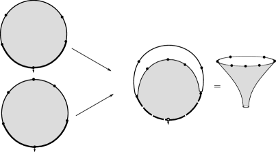
Figure 12. An example of the gluing $\pi_{\mathfrak{S}}$ associated to a $\{(1,1),(k,l)\}$ boundary identification.

Proposition 7.2.

Let $\mathfrak{S}$ be a boundary identification, with compatible point identification $\mathfrak{T}$. Then, the gluing operation $S\coprod_{\mathfrak{S}}T$ extends to an operation on the Deligne-Mumford compactifications ${}_{\mathfrak{T}}\overline{\mathcal{R}}_{k,l}$.

Proof.

Nodal components of an element $P$ in the Deligne-Mumford compactification ${}_{\mathfrak{T}}\overline{\mathcal{R}}_{k,l}$ can be thought of as nodal tricolored discs, with induced boundary identifications in a manner we have already described. As we have earlier indicated, the $L/R$ forgetful maps applied to $P$ give us unreduced left and right disc trees $(\tilde{S},\tilde{T})$. Boundary identifications descend to these trees, because by definition they were labellings between points colored $LR$. We now perform the above procedure component-wise on this pair to obtain a nodal open-closed string $\tilde{S}\coprod_{\mathfrak{S}}(\tilde{T})$, which potentially has semi-stable/unstable components. Finally, define

(7.69) $$\pi_{\mathfrak{S}}(P):=S\coprod_{\mathfrak{S}}T$$

to be the nodal open-closed string obtained by stabilizing $\tilde{S}\coprod_{\mathfrak{S}}\tilde{T}$. ∎

In the case when the boundary identification $\mathfrak{S}$ is empty, the gluing operation $\pi_{\mathfrak{S}}$ reduces to the projection we defined earlier, where we conjugate the first factor:

(7.70) $$\pi_{\emptyset}:=\pi_{reduce}\circ(-1\times id).$$

7.5. Floer data and operations

Definition 7.16.

A Floer datum for a glued pair of discs $(P,\mathfrak{S})$ is a Floer datum for the resulting open-closed string $\pi_{\mathfrak{S}}(P)$, in the sense of Definition 4.11.

Now, let us assume that our point identification $\mathfrak{T}$ was sequential or cyclic sequential.

Definition 7.17.

A universal and consistent choice of Floer data for glued pairs of discs $\mathbf{D}_{glued}$ is a choice $D_{P,\mathfrak{S}}$ of Floer data in the sense of Definition 7.16 for every $k$, $l$, $(k,l)$ boundary identification $\mathfrak{S}$ and compatible sequential point identification $\mathfrak{T}$, and every representative ${}_{\mathfrak{T},\mathfrak{S}}\overline{\mathcal{R}}_{k,l}$, varying smoothly over ${}_{\mathfrak{T},\mathfrak{S}}\overline{\mathcal{R}}_{k,l}$, whose restriction to a boundary stratum is conformally equivalent to the product of Floer data coming from lower dimensional moduli spaces. Moreover, with regards to the coordinates, Floer data agree to infinite order at the boundary stratum with the Floer data obtained by gluing. Finally, we require that this choice of Floer datum satisfy the following conditions:

(7.71) $$\textrm{The Floer datum only depends on the open-closed string }\pi_{\mathfrak{S}}(P);\textrm{ and}$$

(7.72) $$\textrm{The Floer datum agrees with our previously chosen Floer datum on }\pi_{\mathfrak{S}}(P).$$

Definition 7.18.

A Lagrangian labeling from $\mathbf{L}$ for a glued pair of discs $(P,\mathfrak{S})$ is a Lagrangian labeling from $\mathbf{L}$ for the gluing $\pi_{\mathfrak{S}}(P)=S\coprod_{\mathfrak{S}}T$, thought of as a (possibly disconnected) open-closed string. Given a fixed labeling $\vec{L}$, denote by

(7.73) $$(_{\mathfrak{T},\mathfrak{S}}\overline{\mathcal{R}}_{k,l})_{\vec{L}}$$

the space of labeled $\mathfrak{S}$-identified pairs of discs with $\mathfrak{T}$ point coincidences.

Now, fix a compact oriented submanifold with corners of dimension $d$,

(7.74) $$\overline{\mathcal{L}}^{d}\lhook\joinrel\relbar\joinrel\rightarrow{{}_{\mathfrak{T},\mathfrak{S}}}\overline{\mathcal{R}}_{k,l}$$

Fix a Lagrangian labeling

(7.75) $$\vec{L}=\{\{L_{0}^{1},\ldots,L_{m_{1}}^{1}\},\{L_{0}^{2},\ldots,L_{m_{2}}^{2}\},\ldots,\{L_{0}^{h},\ldots,L_{m_{h}}^{h}\}\}.$$

Also, fix chords

(7.76) $$\vec{x}=\{\{x_{1}^{1},\ldots,x_{m_{1}}^{1}\},\ldots,\{x_{1}^{h},\ldots,x_{m_{h}}^{h}\}\}$$

and orbits $\vec{y}=\{y_{1},\ldots,y_{n}\}$ with

(7.77) $$x_{i}^{j}\in\begin{cases}\chi(L_{i+1}^{j},L_{i}^{j})&i\in K^{j}\\ \chi(L_{i}^{j},L_{i+1}^{j})&\mathrm{otherwise.}\end{cases}$$

Above, the index $i$ in $L_{i}^{j}$ is counted mod $m_{j}$. Collectively, the $\vec{x},\vec{y}$ are called a set of asymptotic conditions for the labeled moduli space $\mathcal{L}^{d}_{\vec{L}}$. The outputs $\vec{x}_{out}$, $\vec{y}_{out}$ are by definition those $x_{i}^{j}$ and $y_{s}$ for which $i\in K^{j}$ and $s\in\mathbf{I}$, corresponding to negative marked points. The inputs $\vec{x}_{in}$, $\vec{y}_{in}$ are the remaining chords and orbits from $\vec{x}$, $\vec{y}$. Fixing a chosen universal and consistent Floer datum, denote $\epsilon^{i,j}_{\pm}$ and $\delta^{l}_{\pm}$ the strip-like and cylindrical ends corresponding to $x_{i}^{j}$ and $y_{l}$ respectively.

Finally, define

(7.78) $$\overline{\mathcal{L}}^{d}(\vec{x}_{out},\vec{y}_{out};\vec{x}_{in},\vec{y}_{in})$$

to be the space of maps

(7.79) $$\{u:\pi_{\mathfrak{S}}(P)\longrightarrow M:\ P\in\overline{\mathcal{L}}^{d}\}$$

satisfying, at each element $P$, Floer’s equation for $(\mathbf{D}_{\mathfrak{S}})_{P}$ with boundary and asymptotic conditions

(7.80) $$\begin{cases}\lim_{s\rightarrow\pm\infty}u\circ\epsilon^{i,j}_{\pm}(s,\cdot)=x_{i}^{j},\\ \lim_{s\rightarrow\pm\infty}u\circ\delta^{l}_{\pm}(s,\cdot)=y_{l},\\ \ \ \ u(z)\in\psi^{a_{S}(z)}L_{i}^{j},&z\in\partial_{i}^{j}S.\end{cases}$$

We have the usual transversality and compactness results:

Lemma 7.1.

The moduli spaces $\overline{\mathcal{L}}^{d}(\vec{x}_{out},\vec{y}_{out};\vec{x}_{in},\vec{y}_{in})$ are compact and there are only finitely many collections $\vec{x}_{out}$, $\vec{y}_{out}$ for which they are non-empty given input $\vec{x}_{in}$, $\vec{y}_{in}$. For a generic universal and conformally consistent Floer data they form manifolds of dimension

(7.81) $$\begin{split}\dim\mathcal{L}^{d}(\vec{x}_{out},\vec{y}_{out};\vec{x}_{in},\vec{y}_{in}):=\sum_{x_{-}\in\vec{x}_{out}}&\deg(x_{-})+\sum_{y_{-}\in\vec{y}_{out}}\deg(y_{-})\\ +(2-h(k,l,\mathfrak{S})-|\vec{x}_{out}|-2|\vec{y}_{out}|)n&+d-\sum_{x_{+}\in\vec{x}_{in}}\deg(x_{+})-\sum_{y_{+}\in\vec{y}_{in}}\deg(y_{+}).\end{split}$$

Proof.

The index computation follows from the arguments outlined in the proof of Lemma 4.3. The proof of transversality for generic perturbation data is once more an application of Sard-Smale, following arguments in [Seidel:2008zr]*(9k) or alternatively [Floer:1995fk]. These arguments show that the extended linearized operator for Floer’s equation, in which one allows deformations of the almost complex structure and one-form, is surjective. As their arguments are on the level of stabilized moduli spaces, they imply that transversality can be achieved in our situation by taking perturbations of Floer data that are constant along the fibers of the projection map $\pi_{\mathfrak{S}}$. In other words, the class of Floer data satisfying (7.71) is large enough to achieve transversality.

The usual Gromov compactness applies once Theorem A.1 is applied to obtain a priori bounds on maps satisfying Floer’s equation with fixed asymptotics. ∎

When the dimension of $\mathcal{L}^{d}(\vec{x}_{out},\vec{y}_{out};\vec{x}_{in},\vec{y}_{in})$ is 0, we conclude that its elements are rigid. In particular, any such element $u\in\mathcal{L}^{d}(\vec{x}_{out},\vec{y}_{out};\vec{x}_{in},\vec{y}_{in})$ gives (by Lemma B.1) an isomorphism of orientation lines

(7.82) $$\mathcal{L}_{u}:\bigotimes_{x\in\vec{x}_{in}}o_{x}\otimes\bigotimes_{y\in\vec{y}_{in}}o_{y}\longrightarrow\bigotimes_{x\in\vec{x}_{out}}o_{x}\otimes\bigotimes_{y\in\vec{y}_{out}}o_{y}.$$

Using this we define a map

(7.83) $$\begin{split}\mathbf{G}_{\overline{\mathcal{L}}^{d}}:\bigotimes_{(i,j);1\leq i\leq m_{j};i\notin K^{j}}&CW^{*}(L_{i}^{j},L_{i+1}^{j})\otimes\bigotimes_{1\leq k\leq n;k\notin\mathbf{I}}CH^{*}(M)\longrightarrow\\ &\bigotimes_{(i,j);1\leq i\leq m_{j};i\in K^{j}}CW^{*}(L_{i+1}^{j},L_{i}^{j})\otimes\bigotimes_{1\leq k\leq n;k\in\mathbf{I}}CH^{*}(M)\mbox{ }\end{split}$$

given by, as usual (abbreviating $\vec{x}_{in}=\{x_{1},\ldots,x_{s}\}$, $\vec{y}_{in}=\{y_{1},\ldots,y_{t}\}$)

(7.84) $$\begin{split}&\mathbf{G}_{\overline{\mathcal{L}}^{d}}([y_{t}],\ldots,[y_{1}],[x_{s}],\ldots,[x_{1}]):=\\ &\sum_{\dim\mathcal{L}^{d}(\vec{x}_{out},\vec{y}_{out};\vec{x}_{in},\vec{y}_{in})=0}\sum_{u\in\mathcal{L}^{d}(\vec{x}_{out},\vec{y}_{out};\vec{x}_{in},\vec{y}_{in})}\mathcal{L}_{u}([x_{1}],\ldots,[x_{s}],[y_{1}],\ldots,[y_{t}]).\end{split}$$

This construction naturally associates, to any submanifold $\mathcal{L}^{d}\in{{}_{\mathfrak{S},\mathfrak{T}}}\mathcal{R}_{k,l}$, a map $\mathbf{G}_{\mathcal{L}^{d}}$, depending on a sufficiently generic choice of Floer data for glued pairs of discs. In a similar fashion, this can be done for a submanifold of the labeled space

(7.85) $$\mathcal{L}^{d}_{\vec{L}}\subset(_{\mathfrak{S},\mathfrak{T}}\mathcal{R}_{k,l})_{\vec{L}},$$

in which case the result is an operation defined only for a specific labeling,

(7.86) $$\mathbf{G}_{\overline{\mathcal{L}}^{d}_{\vec{L}}},$$

This operation can also be constructed with a sign twisting datum to create an operation

(7.87) $$(-1)^{\vec{t}}\mathbf{G}_{\overline{\mathcal{L}}^{d}}$$

in an identical fashion to (4.30).

7.6. Examples

As a first example, consider the case $\mathfrak{S}=\emptyset$ and $\mathcal{L}$ equal to the full $\overline{\mathcal{R}}_{k,l}$.

Proposition 7.3.

The operation associated to $\mathcal{L}=\overline{\mathcal{R}}_{k,l}$ with arbitrary Lagrangian labeling is zero if both $k$ and $l$ are $\geq 1$ and one of $(k,l)$ is $\geq 2$.

Proof.

Let $u$ be a rigid element in the associated moduli space $\overline{\mathcal{R}}_{k,l}(\vec{x}_{in};\vec{x}_{out})$; since we are in the transverse situation, we can assume the domain of $u$ is a point in the interior $p\in\mathcal{R}_{k,l}$. On the interior, the projection map

(7.88) $$\pi_{\emptyset}:\mathcal{R}_{k,l}\longrightarrow\mathcal{R}^{k}\times\mathcal{R}^{l}$$

has fibers of dimension at least 1, parametrized by automorphisms of one factor relative to the other. (when $k=1$, we implicitly replace $\mathcal{R}^{k}$ by a point, and same for $l$—stabilization in this case completely collapses the left or right component). Since our Floer data was chosen to only depend on $\pi_{\emptyset}(p)$, we conclude that any map from an element of the fiber $\pi^{-1}_{\emptyset}(\pi_{\emptyset}(p))$ also satisfies Floer’s equation; hence $u$ cannot be rigid. ∎

Proposition 7.4.

The operation associated to the compactification of the inclusion $\mathcal{I}_{k}$ in (7.8) is $(\mu^{k}_{\mathcal{W}})^{op}\otimes id$. Similarly the operation associated to $\mathcal{J}_{l}$ as in (7.9) is $id\otimes\mu^{l}_{\mathcal{W}}$.

Proof.

A rigid element $u$ of the moduli space associated to $\overline{\mathrm{im}(\mathcal{I}_{k})}$ has, without loss of generality, domain in the interior $\mathrm{im}(\mathcal{I}_{k})$. We note that the projection map

(7.89) $$\pi_{\emptyset}:\mathrm{im}(\mathcal{I}_{k})\rightarrow\mathcal{R}^{k}\times\{*\}$$

is an isomorphism up to conjugation. Since we have chosen Floer data compatibly, we obtain an isomorphism

(7.90) $$\overline{\mathcal{I}_{k}(\mathcal{R}^{k})}((x_{0},x_{0}^{\prime});((x_{1},\ldots,x_{k}),x_{0}^{\prime}))\simeq\mathcal{R}^{k}(x_{0};x_{k},\ldots,x_{1})\times\{*\},$$

implying the result for $\mathcal{I}_{k}$. The result for $\mathcal{J}_{l}$ is analogous. ∎

More generally, one can look at the submanifold $\mathcal{Q}_{2}^{k,l}\subseteq\mathcal{R}_{k,l}$ of pairs of discs where the negative marked points are required to coincide and the marked points immediately counterclockwise are required to coincide.

Proposition 7.5.

The associated operation is zero unless $k=1$ or $l=1$, in which case the previous proposition applies.

Proof.

In this case, the projection

(7.91) $$\pi_{\emptyset}:\mathcal{Q}_{2}^{k,l}\longrightarrow\mathcal{R}^{k}\times\mathcal{R}^{l}$$

has one dimensional fibers, parametrized by automorphism of one factor relative another. We conclude in the manner of the previous two propositions that elements of the associated moduli spaces can never be rigid. ∎

We can also look at the submanifold

(7.92) $${}_{\emptyset,\mathfrak{T}}\mathcal{R}_{k,l}$$

of pairs of discs corresponding to the point identification

(7.93) $$\mathfrak{T}=\{(1,1),(2,2)\},$$

i.e. discs where the negative point, and first two positive points, are required to coincide. This submanifold can be thought of as the image of an open embedding from the pair of associahedra

(7.94) $$\mathcal{R}^{r}\times\mathcal{R}^{s}\stackrel{{\scriptstyle Q}}{{\longrightarrow}}\mathcal{R}_{r,s}$$

which can be described as follows: Take the representative of each disc on the left $(-S_{1},S_{2})$ for which the negative marked point and the two marked points immediately counterclockwise of $(S_{1},S_{2})$ have been mapped to $-i$, $1$, and $i$ respectively. Define

(7.95) $$Q([S_{1}],[S_{2}]):=[(S_{1},S_{2})].$$

In other words, associate to a pair of discs mod automorphism the pair mod simultaneous automorphism in which the output and the first two inputs are required to coincide. The embedding $Q$ not quite extend to an embedding of $\overline{\mathcal{R}^{r}}\times\overline{\mathcal{R}^{s}}$ because, among other phenomena, the three chosen points on each disc will come together simultaneously in codimension 1. We can still study the operation determined by the compactification of the embedding.

Proposition 7.6.

The operation associated to the compactification $\overline{Q(\mathcal{R}^{r}\times\mathcal{R}^{s})}$ is $(\mu^{r})^{op}\otimes\mu^{s}$.

Proof.

The map $Q$ is a left and right inverse to the projection map

(7.96) $$\pi_{\emptyset}:_{\emptyset,\{(1,1),(2,2)\}}\mathcal{R}_{k,l}\longrightarrow\mathcal{R}^{k}\times\mathcal{R}^{l}$$

so $\pi_{\emptyset}$ is an isomorphism, up to direction reversal of first factor. We conclude that there is an identification of dimension zero moduli spaces

(7.97) $$\overline{\mathrm{im}(Q)}(x^{1}_{out},x^{2}_{out};\vec{x}^{1}_{in},\vec{x}^{2}_{in})\simeq\overline{\mathcal{R}}^{k}(x^{1}_{out};(\vec{x}^{1}_{in})^{op})\times\overline{\mathcal{R}}^{l}(x^{2}_{out};\vec{x}^{2}_{in}).$$

where the op superscript indicates an order reversal. ∎

Now, consider the case of a single gluing adjacent to the outgoing marked points, i.e. $\mathfrak{S}=\{(1,1)\}$ or $\mathfrak{S}=\{(k,l)\}$ with the induced point identification.

Proposition 7.7.

The resulting operation in either case is $\mu^{k+l+1}$.

Proof.

We will without loss of generality do $\mathfrak{S}=\{(1,1)\}$; the associated point identification is also $p(\mathfrak{S})=\{(1,1)\}$. The gluing morphism is of the form

(7.98) $$\pi_{\mathfrak{S}}:_{\mathfrak{S},p(\mathfrak{S})}\mathcal{R}_{k,l}\longrightarrow\mathcal{R}^{k+l+1}.$$

if $k$ or $l$ is $\geq 1$, the unreduced gluing is automatically stable, implying that (7.98) is an isomorphism. We obtain a corresponding identification of moduli spaces. ∎

Our next example is the case $\mathfrak{S}=\{(1,1),(k,l)\}$ with the induced point identification.

Proposition 7.8.

The resulting operation is exactly ${{}_{2}}\mathcal{OC}^{k-2,l-2}$.

Proof.

The surface obtained by gluing the $(1,1)$ and $(k,l)$ boundary components together in $\mathcal{R}_{k,l}$ is stable, and has one interior output marked point. There are also $k+l$ boundary marked points, two of which are special. In cyclic order on the boundary, there is the identified point $p_{1}$ coming from the $(1,1)$ boundary points, the $k-2$ non-identified points from the left disc, the identified point $p_{2}$ coming from the $(k,l)$ boundary points, and the $l-2$ non-identified points from the right disc. Moreover, the identified points $p_{1}$, $p_{2}$, and the interior boundary point are required to, up to equivalence, lie at the points $-i$, $0$, and $i$ respectively. We conclude that the projection is an isomorphism onto

(7.99) $$\pi_{\mathfrak{S}}:{{}_{\mathfrak{S},p(\mathfrak{S})}}\mathcal{R}_{k,l}\longrightarrow\mathcal{R}^{1}_{k-2,l-2},$$

the moduli space controlling ${{}_{2}}\mathcal{OC}^{k-2,l-2}$.

See also Figure 12 for an image of this situation. ∎

Our final example is the case $\mathfrak{S}=\{(1,1),(2,2)\}$, with the induced point identification.

Proposition 7.9.

The resulting operation is exactly ${{}_{2}}\mathcal{CO}^{k-2,l-2}$.

Proof.

The surface obtained by gluing the $(1,1)$ and $(2,2)$ boundary components together in $\mathcal{R}_{k,l}$ is stable, has one interior input marked point, and in counterclockwise order on the boundary has one output boundary marked point (which was adjacent to the $(1,1)$ gluing), $l-2$ additional boundary inputs, one special boundary input (which was adjacent to the $(2,2)$ gluing), and $k-2$ additional boundary inputs. Moreover, the output boundary marked point, the interior input, and the special boundary input are required to, up to equivalence, lie at the points $-i$, $0$, and $i$ respectively. We conclude that the projection is an isomorphism onto

(7.100) $$\pi_{\mathfrak{S}}:{{}_{\mathfrak{S},p(\mathfrak{S})}}\mathcal{R}_{k,l}\longrightarrow\mathcal{R}^{1,1}_{k-2,l-2},$$

the moduli space controlling ${{}_{2}}\mathcal{CO}^{k-2,l-2}$. ∎

8. Floer theory in the product

The Liouville manifold $M^{2}:=M^{-}\times M$ carries a natural symplectic form, $(-\omega_{M},\omega_{M})$ for which the diagonal is a Lagrangian submanifold. Let

$$\pi_{i}:M^{2}\rightarrow M,\ i=1,2$$

be the projection to the $i$th component. As observed by Oancea [Oancea:2006oq], there is a natural cylindrical end on $M^{-}\times M$, with coordinate given by $r_{1}+r_{2}$, where $r_{i}=\pi_{i}^{*}r$ is the coordinate on the $i$-th factor. Thus one could define symplectic homology and wrapped Floer theory by considering Hamiltonians of the form $(r_{1}+r_{2})^{2}$ at infinity. To obtain the comparisons that we desire, we must consider Floer theory for split Hamiltonians of the form $\pi_{1}^{*}H+\pi_{2}^{*}H$, for $H\in\mathcal{H}(M)$. There are immediately some technical difficulties: split Hamiltonians are not admissible in the above sense, and in general will admit some additional chords near infinity. Using methods similar to [Oancea:2006oq], one could prove that these orbits and chords have sufficiently negative action, do not contribute to the homology, and thus such split Hamiltonians are a posteriori admissible (thereby proving a Künneth theorem for wrapped Floer homology).

We bypass this issue and instead define all Floer-theoretic operations on the product for split Hamiltonians and almost complex structures. In this case, with suitably chosen Floer data, compactness and transversality follow, via unfolding, from compactness and transversality of certain open-closed moduli spaces of maps into $M$ constructed from glued pairs of discs. The end result will be a model

(8.1) $$\mathcal{W}^{2}$$

for the wrapped Fukaya category of split Lagrangians and the diagonal in $M^{2}$, using only maps and morphisms in $M$.

Remark 8.1.

There is another technical difficulty with considering Hamiltonians of the form $(r_{1}+r_{2})^{2}$ at infinity: Products of admissible Lagrangians $L_{i}\times L_{j}$ are no longer a priori admissible in the product. Namely, it is not guaranteed (and highly unlikely) that the primitive $\pi_{1}^{*}f_{L_{i}}+\pi_{2}^{*}f_{L_{j}}$ is constant as $(r_{1}+r_{2})\rightarrow\infty$. The usual method of proving that the relevant moduli spaces are compact does not work in this situation, and a more refined argument is needed.

8.1. Floer homology with split Hamiltonians

First, let us examine Floer homology groups in $M^{2}$ for a class of split Hamiltonians $\tilde{\mathcal{H}}(M\times M)$ of the form

(8.2) $$\pi_{1}^{*}H+\pi_{2}^{*}H,\ H\in\mathcal{H}(M).$$

For Floer homology between split Lagrangians we immediately obtain a Künneth decomposition.

Lemma 8.1.

For $H$ and $J$ generic, there is an identification of complexes

(8.3) $$CW^{*}(L_{1}\times L_{2},L_{1}^{\prime}\times L_{2}^{\prime};\pi_{1}^{*}H+\pi_{2}^{*}H,(-J,J))=CW^{*}(L_{1}^{\prime},L_{1},H,J)\otimes CW^{*}(L_{2},L_{2}^{\prime};H,J)$$

where the differential on the right hand side is $\delta_{L_{1}^{\prime},L_{1}}\otimes 1+1\otimes\delta_{L_{2},L_{2}^{\prime}}$.

Proof.

If $X$ is the Hamiltonian vector field corresponding to $H$, note that the complex on the left-hand side of 8.3 is generated by time 1 flows of the vector field $(-X,X)$, so there is a one-to-one correspondence of generators. By examining equations we see that there is a one-to-one correspondence of strips

(8.4) $$\mathcal{R}^{1}((x_{0},x_{0}^{\prime}),(x_{1},x_{1}^{\prime}))=\mathcal{R}^{1}(x_{0};x_{1})\times\mathcal{R}^{1}(x_{0}^{\prime};x_{1}^{\prime})$$

In particular, the dimension of $\mathcal{R}^{1}((x_{0},x_{0}^{\prime}),(x_{1},x_{1}^{\prime}))$ is

$$\deg x_{0}-\deg x_{1}+\deg x_{0}^{\prime}-\deg x_{1}^{\prime}=\dim\mathcal{R}^{1}(x_{0};x_{1})+\dim\mathcal{R}^{1}(x_{0}^{\prime};x_{1}^{\prime})$$

This implies that the one-dimensional component of the moduli space is the union of

• the one-dimensional component of $\mathcal{R}^{1}(x_{0};x_{1})$ times the zero-dimensional component of $\mathcal{R}^{1}(x_{0}^{\prime};x_{1}^{\prime})$.

• the one-dimensional component of $\mathcal{R}^{1}(x_{0}^{\prime};x_{1}^{\prime})$ times the zero-dimensional component of $\mathcal{R}^{1}(x_{0};x_{1})$.

But by Proposition 6.1, the zero-dimensional component of the above moduli spaces must be constant maps, thereby implying the Lemma. ∎

Floer trajectories with the diagonal Lagrangian $\Delta$ unfold and can be compared to symplectic cohomology trajectories, for appropriate Hamiltonians.

Lemma 8.2.

For $H_{t}$ and $J$ generic,

(8.5) $$CW^{*}(\Delta,\Delta,\pi_{1}^{*}\frac{1}{2}H_{1-t/2}+\pi_{2}^{*}\frac{1}{2}H_{t/2},(-J,J))=CH^{*}(M,H_{t},J)$$

as relatively graded chain complexes.

Proof.

Denote $\hat{H}_{t}=\pi_{1}^{*}\frac{1}{2}H_{1-t/2}+\pi_{2}^{*}\frac{1}{2}H_{t/2}.$ The correspondence between generators is as follows: Given a time 1 orbit $x$ of $H_{t}$, we construct a time 1 chord from $\Delta$ to $\Delta$ of $\hat{H}_{t}$

(8.6) $$\hat{x}(t)=(x(1-t/2),x(t/2)).$$

Conversely, given a time 1 chord $\hat{x}=(x_{1},x_{2})$ of $\hat{H}_{t}$ , the corresponding orbit of $H_{t}$ is given by:

(8.7) $$x(t)=\begin{cases}x_{2}(2t)&t\leq 1/2\\ x_{1}(2(1-t))&1/2\leq t\leq 1\end{cases}$$

Let us now identify the moduli spaces counted by either differential. First, suppose we have a map $u:{\mathbb{R}}\times{\mathbb{R}}/2{\mathbb{Z}}\rightarrow M$ satisfying:

$$\partial_{s}u+J_{t}(\partial_{t}u-X_{t}) =0$$

$$\lim_{s\rightarrow-\infty}u(s,\cdot) =x_{-}$$

$$\lim_{s\rightarrow\infty}u(s,\cdot) =x_{+}$$

where $X_{t}$ is the Hamiltonian vector field corresponding to $H_{t}$. Then, note that the map

(8.8) $$\hat{u}(s,t):=(u_{1}(s,1-t/2),u_{2}(s,t/2))$$

satisfies the equation

(8.9) $$\partial_{s}\hat{u}=-(-J_{1-t/2},J_{1-t/2})\left(\partial_{t}\hat{u}-(-X_{1-t/2},X_{t/2})\right)$$

with limits

(8.10) $$\lim_{s\rightarrow-\infty}\hat{u}(s,\cdot) =\hat{x}_{-},$$

(8.11) $$\lim_{s\rightarrow\infty}\hat{u}(s,\cdot) =\hat{x}_{+}.$$

Conversely, suppose we have a map $\hat{u}:{\mathbb{R}}\times[0,1]\rightarrow M^{-}\times M$ satisfying

(8.12) $$\partial_{s}u+(-J_{1-t/2},J_{1-t/2})(\partial_{t}u-(-X_{1-t/2},X_{t/2})) =0$$

(8.13) $$\lim_{s\rightarrow-\infty}u(s,\cdot) =\hat{x}_{-}$$

(8.14) $$\lim_{s\rightarrow\infty}u(s,\cdot) =\hat{x}_{+}.$$

Let $u_{i}=\pi_{i}\circ\hat{u}$, and define

(8.15) $$u(s,t)=\begin{cases}u_{2}(s,2t)&0\leq t\leq 1/2\\ u_{1}(s,2(1-t))&1/2\leq t\leq 1.\end{cases}$$

Because $\hat{u}(s,0)$ and $\hat{u}(s,1)$ lie on $\Delta$, $u(s,t)$ is continuous across the seams $t=0,\ 1/2$. It is clear that $\partial_{s}u$ is continuous along $t=0,\ 1/2$. Thus, as $u$ solves $\partial_{s}u+J_{t}(\partial_{t}u-X_{t})=0$ on both sides of $t=0$ and $t=1$, we see that $\partial_{t}u$ = $J_{t}(\partial_{s}u)+X_{t}$ is continuous, so $u$ is at least $C^{1}$ across the seams. Now inductively use the fact that $\partial_{s}^{k}$ is continuous for all $k$ along with applications of $\partial_{s}$ and $\partial_{t}$ to Floer’s equation, to conclude that all other mixed partials are continuous. Therefore $u$ is $C^{\infty}$ across the seams. ∎

The cases of $HW^{*}(\Delta,L_{i}\times L_{j})$ and $HW^{*}(L_{i}\times L_{j},\Delta)$ are analogous, so we simply state them.

Proposition 8.1.

As relatively graded chain complexes,

(8.16) $$CW^{*}(L_{i}\times L_{j},\Delta,\frac{1}{2}(\pi_{1}^{*}H+\pi_{2}^{*}H),(-J,J))=CW^{*}(L_{j},L_{i},H,J)$$

Proposition 8.2.

As relatively graded chain complexes,

(8.17) $$CW^{*}(\Delta,L_{i}\times L_{j},\frac{1}{2}(\pi_{1}^{*}H+\pi_{2}^{*}H),(-J,J))=CW^{*}(L_{i},L_{j},H,J).$$

In the setting of the ordinary Fukaya category, the analogue of Lemma 8.2 is the well-known correspondence between $HF^{*}(\Delta,\Delta)$ with the ordinary Hamiltonian Floer homology, or quantum cohomology, of the target manifold. Instead of continuing this correspondence for higher operations and, e.g. unfolding Floer data for discs mapping into $M^{2}$, we will take the above correspondence as a starting point for a definition of the category $\mathcal{W}^{2}$ using operations and Floer data in $M$. Define the objects of $\mathcal{W}^{2}$ as

(8.18) $$\mathrm{ob\ }\mathcal{W}^{2}:=\{L_{i}\times L_{j}|L_{i},L_{j}\in\mathrm{ob\ }\mathcal{W}\}\cup\{\Delta\}.$$

For objects $X_{k}$, $X_{l}$, define the generators of the morphism complexes

(8.19) $$\chi_{M^{2}}(X_{k},X_{l}):=\begin{cases}\chi(L_{j},L_{i},H)\times\chi(L_{i}^{\prime},L_{j}^{\prime},H)&X_{k}=L_{i}\times L_{i}^{\prime},\ X_{l}=L_{j}\times L_{j}^{\prime}\\ \chi(L_{j},L_{i})&X_{k}=L_{i}\times L_{j},\ X_{l}=\Delta\\ \chi(L_{i},L_{j})&X_{k}=\Delta,\ X_{l}=L_{i}\times L_{j}\\ \mathcal{O}&X_{k}=X_{l}=\Delta\end{cases}$$

Also, define the differential $\mu^{1}_{\mathcal{W}^{2}}$ to be the differentials coming from the correspondences in the Lemmas above. It remains to define gradings and construct $A_{\infty}$ operations, which we do in reverse order.

8.2. The $A_{\infty}$ category

To complete the construction of $\mathcal{W}^{2}$, we construct higher $A_{\infty}$ operations $\mu^{d}_{\mathcal{W}^{2}}$, $d\geq 2$. First, suppose we have fixed a universal and conformally consistent Floer datum for pairs of glued discs and genus-0 open closed strings. Now, consider the space of labeled associahedra

(8.20) $$\mathcal{R}^{d}_{\mathbf{L}^{2}}$$

with label set the relevant Lagrangians in $M^{2}$:

(8.21) $$\mathbf{L}^{2}=\{\Delta\}\cup\{L_{i}\times L_{j}|L_{i},L_{j}\in\mathrm{ob\ }\mathcal{W}\}.$$

Consider first the case where all Lagrangians are split. Discs in $M^{-}\times M$ solving the inhomogenous Cauchy-Riemann equation with respect to a split Hamiltonian in $\tilde{\mathcal{H}}(M^{-}\times M)$ split almost complex structure $(-J,J)$ and split Lagrangian boundary conditions are exactly pairs of discs $u_{1}$, $u_{2}$ with the same conformal structure (up to conjugation) solving the inhomogenous Cauchy-Riemann equation with respect to $\omega$, $J$ and respective Lagrangian boundary conditions. The relevant moduli space of abstract discs is the diagonal associahedron

(8.22) $$\overline{\mathcal{R}}^{d}\stackrel{{\scriptstyle\Delta_{d}}}{{\lhook\joinrel\relbar\joinrel\rightarrow}}_{\emptyset,\mathfrak{T}_{max}}\overline{\mathcal{R}}_{d,d}.$$

For labeling sequences $\vec{L}^{2}$ from $\mathbf{L}^{2}$ not containing $\Delta$, we can think of $\Delta_{d}$ as an embedding of labeled moduli spaces

(8.23) $$(\Delta_{d})_{\vec{L}^{2}}:(\mathcal{R}^{d})_{\vec{L}^{2}}\longrightarrow(\mathcal{R}_{d,d})_{\mathbf{L}}$$

in the obvious manner: if a boundary component of $S\in\overline{\mathcal{R}}^{d}_{\mathbf{L}^{2}}$ was labeled $L_{i}\times L_{j}$, applying $\Delta_{d}$, label the respective component of the first factor $L_{i}$ and the second component $L_{j}$.

Definition 8.1.

Define the operation $\mu^{d}_{\mathcal{W}^{2}}$, for sequences of Lagrangians $\vec{L}^{2}$ in $\mathbf{L}^{2}$ not containing $\Delta$, to be the operation controlled by the image of $(\Delta_{d})_{\vec{L}^{2}}$ as in Equation (7.86), with sign twisting datum given by the image of the sequential sign twisting datum

(8.24) $$\vec{t}_{d}=(1,\ldots,d)$$

in the following sense: twist inputs in the image of $(\Delta_{d})_{\vec{L}^{2}}$ of a boundary point $z_{j}$ by weight $j$.

Now, let us give a more general construction of the operations, for cases including $\Delta$. Let $S$ be a disc in $\mathcal{R}^{d}$ with labels $\vec{L}^{2}$ from $\mathbf{L}^{2}$, with at least one label equal to $\Delta$. Let

(8.25) $$D(\vec{L}^{2})$$

be the set of indices of boundary components of $S$ labeled $\Delta$. Then, let

(8.26) $$\mathfrak{T}_{max}=\{(1,1),(2,2),\ldots,(d,d)\}$$

be the maximal boundary identification data and let

(8.27) $$\mathfrak{S}(\mathbf{L}^{2})=\{(i,i)|i\in D(\vec{L}^{2})\}$$

be the set of boundary components determined by the positions of $\Delta$. Finally, define

(8.28) $$\mathbf{\Phi}_{\vec{L}^{2}}(\mathcal{R}^{d}):=_{\mathfrak{S}(\mathbf{L}^{2}),\mathfrak{T}_{max}}\mathcal{R}_{d,d}$$

Label the boundary components of the resulting pair of discs as follows: if $\partial_{k}S$ was labeled $L_{i}\times L_{j}$, then in $\mathbf{\Phi}_{\vec{L}}(S)$, the left image of $\partial_{k}S$ will be labeled $L_{i}$ and the right of $\partial_{k}S$ will be labeled $L_{j}$. If $\partial_{k}S$ was labeled $\Delta$, then it will become part of a boundary identification and disappear under gluing so there is nothing to label.

Definition 8.2.

Define the operation

(8.29) $$\mu^{d}_{\mathcal{W}^{2}},$$

for sequences of Lagrangians $\vec{L}^{2}$ in $\mathbf{L}^{2}$, to be the operation controlled by the image of $\mathbf{\Phi}_{\vec{L}^{2}}$ as in Equation (7.86).

Figure 13. An example of the labeled gluing $\mathbf{\Phi}_{\vec{L}^{2}}$.

Because the unfolding maps $\mathbf{\Phi}_{\vec{L}^{2}}$ are embeddings of associahedra,

Proposition 8.3.

The operations $\mu^{d}_{\mathcal{W}^{2}}$ as constructed satisfy the $A_{\infty}$ equations.

8.3. Gradings

The identifications of chain complexes in Section 8.1 give us an identification of complexes with relative grading. In this section, we would like to make the subtle observation that naively attempting to inherit the absolute grading from $M$ under these identifications will result in the $A_{\infty}$ operations having the wrong degree.

Proposition 8.4.

Fix a choice of gradings in $M$. Then, choose gradings for $M^{2}$ in the following manner: given correspondences of generators for morphism complexes

(8.30) $$\begin{split}\chi_{M^{2}}(L_{0}\times L_{1},L_{0}^{\prime}\times L_{1}^{\prime})&\longleftrightarrow\chi(L_{0}^{\prime},L_{0})\times\chi(L_{1},L_{1}^{\prime})\\ x&\longleftrightarrow\hat{x}=(x_{1},x_{2})\end{split}$$

(8.31) $$\begin{split}\chi_{M^{2}}(L_{0}\times L_{1},\Delta)&\longleftrightarrow\chi(L_{1},L_{0})\\ z&\longleftrightarrow\hat{z}\end{split}$$

(8.32) $$\begin{split}\chi_{M^{2}}(\Delta,L_{0}\times L_{1})&\longleftrightarrow\chi(L_{0},L_{1})\\ w&\longleftrightarrow\hat{w}\end{split}$$

(8.33) $$\begin{split}\chi_{M^{2}}(\Delta,\Delta)&\longleftrightarrow\mathcal{O}\\ y&\longleftrightarrow\hat{y}\end{split}$$

assign gradings as follows:

(8.34) $$\deg x =\deg\hat{x}=\deg x_{1}+\deg x_{2}$$

(8.35) $$\deg z =\deg\hat{z}$$

(8.36) $$\deg w =\deg\hat{w}+n$$

(8.37) $$\deg y =\deg\hat{y}.$$

For this choice, the operations $\mu^{d}_{\mathcal{W}^{2}}$ constructed in the previous section are of degree $2-d$, thus forming an $A_{\infty}$ structure.

Proof.

There are two proofs of this fact. In the first, we can treat the numbers $\deg(x)$, $\deg(y)$ as black boxes and verify that the degree assignment given above makes the $A_{\infty}$ operations $\mathcal{W}^{2}$ have correct degree $2-d$ for any sequence of labeled Lagrangians. This could be done as follows: Take an arbitrary labeling $\vec{L}^{2}$ of Lagrangians, some of which are $\Delta$ and some of which are $L_{i}\times L_{j}$’s, and calculate the number of boundary components, number of boundary outputs, and number of interior outputs of the resulting open-closed string $\pi_{\mathfrak{S}}(\mathbf{\Phi}_{\vec{L}^{2}}(S))$, thus arriving at the dimension (and therefore degree) of the operation controlled by $\mathbf{\Phi}_{\vec{L}^{2}}$. The main observation here is that, inductively, any sequence of consecutive labels of $\Delta$ that do not appear at the end of the sequence shift the index by $n$, either by gluing a pair of discs together for the first time, by adding an additional boundary component or or by turning a boundary output into an interior output (note that interior outputs are only formed if there are $\Delta$ labels on both ends, an edge case). Correspondingly, any such sequence contributes a term of the form $\hom(\Delta,L_{i}\times L_{j})$. Thus in terms of the grading given above, the operation continues to have degree $2-d$.

Alternatively, we give a conceptual argument, assuming that $M$ is a compact manifold. Suppose we had chosen a grading for $\Delta$ such that $\hom(L_{1}\times L_{2},\Delta)\simeq\hom(L_{1},L_{2})$ as graded complexes. Then, by Poincaré duality on $M^{2}$ then on $M$, we must have that

(8.38) $$\hom(\Delta,L_{1}\times L_{2})\simeq\hom(L_{1}\times L_{2},\Delta)^{\vee}[2n]\simeq\hom(L_{2},L_{1})^{\vee}[2n]\simeq\hom(L_{1},L_{2})[n].$$

Of course, Poincaré duality fails in our situation, but this argument gives a reasonable sanity check regarding gradings. ∎

9. From the product to bimodules

9.1. Moduli spaces of quilted strips

The next three definitions are due to Ma’u [Mau:2010lq]:

Definition 9.1.

Fix $-\infty<x_{1}<x_{2}<x_{3}<\infty$. A 3-quilted line consists of the three parallel lines $l_{1},l_{2},l_{3}$, each of which is a vertical line $\{x_{j}+i{\mathbb{R}}\}$ considered as a subset of $[x_{1},x_{3}]\times(-\infty,\infty)\subset{\mathbb{C}}$.

Definition 9.2.

Let $\mathbf{r}=(r_{1},r_{2},r_{3})\in{\mathbb{Z}}^{3}_{\geq 0}$. A 3-quilted line with $\mathbf{r}$ markings consists of the data $(Q,\mathbf{z}_{1},\mathbf{z}_{2},\mathbf{z}_{3})$, where $Q$ is a 3-quilted line, and each vector $\mathbf{z}_{i}=(z^{1}_{i},\ldots,z^{r_{i}}_{i})$ is an upwardly ordered configuration of points in $l_{i}$, i.e. $\mathrm{Re}(z_{i}^{k})=l_{i}$ and $-\infty<\mathrm{Im}(z_{i}^{1})<\mathrm{Im}(z_{i}^{2})<\cdots<\mathrm{Im}(z_{i}^{r_{i}})<\infty$.

There is a free and proper ${\mathbb{R}}$ action on such quilted lines with markings, given by simultaneous translation in the ${\mathbb{R}}$ direction.

Definition 9.3.

The moduli space of 3-quilted, $\mathbf{r}$-marked strips $Q(3,\mathbf{r})$ is the set of such 3-quilted lines with $\mathbf{r}$ markings, modulo translation.

Figure 14. A quilted strip with $(3,5,2)$ markings.

Ma’u also gives a description of the Deligne-Mumford compactification

$$\overline{Q(3,\mathbf{r})}$$

of the above moduli space, the moduli space of stable, nodal 3-quilted lines with $\mathbf{r}$ markings. Strata consist of multi-level broken 3-quilted lines with stable discs glued to marked points on each of the three lines at any level. The manifold with corners structure near these strata comes from gluing charts, which are similar to ones we have already written down. We refer the reader to [Mau:2010lq]*§2 for more details on this moduli space, but in codimension 1

Proposition 9.1.

The boundary $\partial\overline{Q(3,\mathbf{r}=(r_{1},r_{2},r_{3}))}$ is covered by the images of the codimension 1 inclusions

(9.1) $$\begin{split}\overline{Q(3,(a,b,c))}\times\overline{Q(3,(r_{1}-a,r_{2}-b,r_{3}-c))}&\rightarrow\partial\overline{Q(3,\mathbf{r})}\\ \overline{Q(3,(a+1,r_{2},r_{3}))}\times\overline{\mathcal{R}^{r_{1}-a}}&\rightarrow\partial\overline{Q(3,\mathbf{r})}\\ \overline{Q(3,(r_{1},b+1,r_{3}))}\times\overline{\mathcal{R}^{r_{2}-b}}&\rightarrow\partial\overline{Q(3,\mathbf{r})}\\ \overline{Q(3,(r_{1},r_{2},c+1))}\times\overline{\mathcal{R}^{r_{3}-c}}&\rightarrow\partial\overline{Q(3,\mathbf{r})}.\end{split}$$

We will use the open space $Q(3,\mathbf{r})$ to construct operations controlled by various glued pairs of discs. The codimension 1 compactification of the resulting moduli spaces we consider will not quite be (9.1), but will only differ by some strata whose associated operations are zero.

Definition 9.4.

Let $\mathbf{L}_{1}$, $\mathbf{L}_{2}$, $\mathbf{L}_{3}$ be sets of Lagrangians in $M$, $M^{2}$, and $M$ respectively. A Lagrangian labeling from $(\mathbf{L}_{1},\mathbf{L}_{2},\mathbf{L}_{3})$ for a 3-quilted line with $\mathbf{r}$ markings $(Q,\mathbf{z}_{1},\mathbf{z}_{2},\mathbf{z}_{3})$ consists of, for each $i$, an assignment of a label in $\mathbf{L}_{i}$ to each of the $r_{i}+1$ components of the punctured line $l_{i}-\mathbf{z}_{i}$. The space of 3-quilted lines with $\mathbf{r}$-markings and $(\mathbf{L}_{1},\mathbf{L}_{2},\mathbf{L}_{3})$ labels is denoted $Q(3,\mathbf{r})_{(\mathbf{L}_{1},\mathbf{L}_{2},\mathbf{L}_{3})}$.

9.2. Unfolding labeled quilted strips

Fix the label set $\hat{\mathbf{L}}=(\mathbf{L},\mathbf{L}^{2},\mathbf{L})$. Let $S$ be a stable labeled, 3-quilted strip with $\mathbf{r}$-markings, $S\in Q(3,\mathbf{r})_{\hat{\mathbf{L}}}$, labeled by $\hat{\vec{L}}=(\vec{L}_{0},\vec{L}^{2},\vec{L}_{1})$. We associate to $S$ a pair of glued discs

(9.2) $$\mathbf{\Psi}_{\hat{\vec{L}}}(S).$$

in a manner analogous to the construction of $\mathbf{\Psi}$ in Section 8.2. From a 3-quilted line with marked points $S$, consider the substrips $-S_{1}$ and $S_{2}$, where $S_{i}$ is $(i=1,2)$ given by the regions in between and including lines $l_{i}$ and $l_{i+1}$ ($-S_{1}$ denotes the reflection of $S_{1}$ across a vertical axis).

$-S_{1}$ and $S_{2}$ are conformally discs with boundary marked points $\mathbf{z}_{i}\cup\mathbf{z}_{i+1}\cup\{a_{i}^{\pm}\}$, where $a_{i}^{\pm}$ are the marked points corresponding in the strip-picture to $\pm\infty$. Denote the connected components of the line $l_{2}-\mathbf{z}_{2}$ by $\partial_{j}^{2}S$, $j=1,\ldots,r_{2}+1$, and the images of these boundary components in $S_{i}$ by $\partial_{j}^{2}S_{i}$. Pick some conformal map $\phi$ from the strip to a disc with marked points at $\pm\infty$ sent to $\pm 1$. Apply this same conformal map to $-S_{1}$ and $S_{2}$ and call the results $-\tilde{S}_{1}$, $\tilde{S}_{2}$. By construction $\tilde{S}_{1}$ and $\tilde{S}_{2}$ have $r_{2}+1$ coincident points

(9.3) $$\mathfrak{T}=\{(1,1),\ldots,(r_{2}+1,r_{2}+1)\}$$

coming from the marked points on the strip $l_{2}$ and the point at $+\infty$.

Now, define the boundary identification

(9.4) $$\mathfrak{S}(\hat{\vec{L}}):=\{(i,i)|1\leq i\leq r_{2}+1,\ \partial_{i}^{2}S\mathrm{\ is\ labeled\ }\Delta\}.$$

Thus, we can define

(9.5) $$\mathbf{\Psi}_{\hat{\vec{L}}}(Q(3,(r_{1},r_{2},r_{3}))):={{}_{\mathfrak{S}(\hat{\vec{L}}),\mathfrak{T}}}\overline{\mathcal{R}}_{r_{2}+r_{1}+1,r_{2}+r_{3}+1}.$$

The resulting space is labeled as follows: The connected components of $l_{i}-z_{i}$ for $i=1,3$ in the image of $\mathbf{\Psi}$ retain the same labeling. If $\partial^{2}_{j}S$ was labeled by some $L_{s}\times L_{t}$, then label the image of $\partial^{2}_{j}S_{1}$ by $L_{s}$ and the image of $\partial^{2}_{j}S_{2}$ by $L_{t}$.

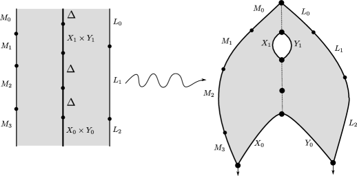
Figure 15. An example of the quilt unfolding $\mathbf{\Psi}_{\hat{\vec{L}}}$.

9.3. The $A_{\infty}$ functor

Using the above embeddings of labeled moduli spaces, we construct an $A_{\infty}$ functor

(9.6) $$\mathbf{M}:\mathcal{W}^{2}\longrightarrow\mathcal{W}\mathrm{\!-\!mod\!-\!}\mathcal{W}.$$

On an object $X\in\mathcal{W}^{2}$, the bimodule $\mathbf{M}(X)$ is specified by the following data:

• for pairs of objects $A,B\in\mathrm{ob\ }\mathcal{W}$, $\mathbf{M}(X)(A,B)$ is generated as a graded vector space by $\chi_{M^{2}}(A\times B,X)$, which we recall to be:

  (9.7) $$\begin{cases}\chi(L_{1},A)\times\chi(B,L_{2})&X=L_{1}\times L_{2}\\ \chi(B,A)&X=\Delta\end{cases}$$

• differential

  (9.8) $$\mu^{0|1|0}_{\mathbf{M}}:\mathbf{M}(X)(L,L^{\prime})\longrightarrow\mathbf{M}(X)(L,L^{\prime})$$

  which is exactly the differential $\mu^{1}_{\mathcal{W}^{2}}$ on $\hom_{\mathcal{W}^{2}}(L\times L^{\prime},X)$, counting pairs of strips modulo simultaneous automorphisms.

• for objects $(A_{0},\ldots,A_{r},B_{0},\ldots,B_{s})$, higher bimodule structure maps

  (9.9) $$\begin{split}\mu^{r|1|s}_{\mathbf{M}}:&\hom_{\mathcal{W}}(A_{r-1},A_{r})\times\cdots\hom_{\mathcal{W}}(A_{0},A_{1})\times\mathbf{M}(X)(A_{0},B_{0})\times\\ &\times\hom_{\mathcal{W}}(B_{1},B_{0})\times\cdots\times\hom_{\mathcal{W}}(B_{s},B_{s-1})\longrightarrow\mathbf{M}(X)(A_{r},B_{s}).\end{split}$$

  These maps are the ones determined by the moduli space

  (9.10) $$\overline{\mathbf{\Psi}_{\hat{\vec{L}}}(Q(3,(r,0,s))_{\hat{\vec{L}}})}$$

  in the sense of equations (4.31) and (7.86), where

  (9.11) $$\hat{\vec{L}}=((A_{0},\ldots,A_{r}),(X),(B_{0},\ldots,B_{s})),$$

  using existing choices of Floer data and sign twisting datum

  (9.12) $$\vec{t}=(1,2,\ldots,s,s,s+1,\ldots,s+r)$$

  with respect to the reverse ordering of inputs in (9.9) (considering $\mathbf{M}(X)(A_{0},B_{0})$ as a single input).

The consistency condition imposed on the choice of Floer data pairs of glued discs and the codimension-1 strata (9.1) imply that

Proposition 9.2.

$\mathbf{M}(X)$ is an $A_{\infty}$ bimodule.

Proof.

We look at the boundary of the associated one-dimensional moduli spaces. The resulting pair of glued discs has a sequential point identification $\mathfrak{T}=\{(1,1),(2,2)\}$. We have already examined the boundary strata of ${}_{\mathfrak{S}(\hat{\vec{L}}),\mathfrak{T}}\mathcal{R}_{r+1+1,r_{3}+1}$ in Proposition 7.1. The composed operations corresponding to stratas (7.53) - (7.55) vanish by Proposition 7.3. The strata (7.52), (7.56), and (7.57) correspond exactly to equations of the form

(9.13) $$\begin{split}\mu_{\mathbf{M}(X)}(\cdots\mu_{\mathbf{M}(X)}(\cdots,\mathbf{b},\cdots),\cdots),\\ \mu_{\mathbf{M}(X)}(\cdots,\mathbf{b},\cdots\mu_{\mathcal{W}}(\cdots),\cdots),\\ \mu_{\mathbf{M}(X)}(\cdots,\mu_{\mathcal{W}}(\cdots),\cdots,\mathbf{b},\cdots,\cdots)\end{split}$$

respectively, which together comprise the terms of the $A_{\infty}$ bimodule relations. There are final terms coming from strip-breaking, corresponding to allowing ourselves to apply $\mu^{1}$ or $\mu^{0|1|0}$ before or after applying $\mu_{\mathbf{M}(X)}$. Verification of signs is as in Appendix B. ∎

Given objects $X_{0},\ldots,X_{d}\in\mathcal{W}^{2}$, the higher terms of the functor are maps

(9.14) $$\mathbf{M}^{d}:\hom_{\mathcal{W}}(X_{d-1},X_{d})\otimes\cdots\hom_{\mathcal{W}}(X_{0},X_{1})\longrightarrow\hom_{\mathcal{W}\mathrm{\!-\!mod\!-\!}\mathcal{W}}(\mathbf{M}(X_{0}),\mathbf{M}(X_{d}))$$

sending

(9.15) $$x_{d}\otimes\cdots\otimes x_{1}\longmapsto\mathbf{m}_{(x_{d},\ldots,x_{1})}\in\hom_{\mathcal{W}\mathrm{\!-\!mod\!-\!}\mathcal{W}}(\mathbf{M}(X_{0}),\mathbf{M}(X_{d})).$$

The bimodule homomorphism $\mathbf{m}_{(x_{d},\ldots,x_{1})}$ consists of, for objects $(A_{0},\ldots,A_{r},B_{0},\ldots,B_{s})$ in $\mathcal{W}$, maps:

(9.16) $$\begin{split}\mathbf{m}_{(x_{d},\ldots,x_{0})}^{r|1|s}:&\hom_{\mathcal{W}}(A_{r-1},A_{r})\times\cdots\hom_{\mathcal{W}}(A_{0},A_{1})\times\mathbf{M}(X_{0})(A_{0},B_{0})\times\\ &\times\hom_{\mathcal{W}}(B_{1},B_{0})\times\cdots\times\hom_{\mathcal{W}}(B_{s},B_{s-1})\longrightarrow\mathbf{M}(X_{d})(A_{r},B_{s})\end{split}$$

Letting $\hat{\vec{L}}=((A_{0},\ldots,A_{r}),(X_{0},\ldots,X_{d}),(B_{0},\ldots,B_{s}))$, we define the above operation to be the one controlled in the sense of Equations (4.31) and (7.86) by the unfolded image

(9.17) $$\overline{\mathbf{\Psi}_{\hat{\vec{L}}}(Q(3,(r,d,s))}_{\hat{\vec{L}}})$$

with sign twisting datum

(9.18) $$\vec{t}=(1,\ldots,d,1,\ldots,r,r,r+1,\ldots,r+s)$$

with respect to the ordering of inputs given by $x_{1},\ldots,x_{d}$ followed by the reverse of the order of inputs in (9.16) (as before, this means that we twist the image of the inputs after unfolding by these quantities). The consistency condition for Floer data for open-closed strings and pairs of discs, along with the codimension 1 boundary of quilted strips (9.1) imply

Proposition 9.3.

The data $\mathbf{M}^{d}$ as defined above gives an $A_{\infty}$ functor

(9.19) $$\mathbf{M}:\mathcal{W}^{2}\longrightarrow\mathcal{W}\mathrm{\!-\!mod\!-\!}\mathcal{W}.$$

Proof.

We need to verify the $A_{\infty}$ functor equation, which (as $\mathcal{W}\mathrm{\!-\!mod\!-\!}\mathcal{W}$ is a dg category), takes the form:

(9.20) $$\mu^{1}_{\mathcal{W}\!-\!\mathcal{W}}\circ\mathbf{M}^{d}+\sum_{i_{1}+i_{2}=d}(\mathbf{M}^{i_{1}}``\circ"\mathbf{M}^{i_{2}})=\mathbf{M}\circ\hat{\mu}_{\mathcal{W}}.$$

We examine the boundary strata ${}_{\mathfrak{S}(\hat{\vec{L}}),\mathfrak{T}}\mathcal{R}_{r+d+1,d+r_{3}+1}$ computed in Proposition 7.1, for $\mathfrak{T}=\{(1,1),\ldots,(d+1,d+1)\}$. The first term, $\mu^{1}_{\mathcal{W}\mathrm{\!-\!mod\!-\!}\mathcal{W}}(\mathbf{M}^{d})=\mu_{\mathbf{M}(X_{d})}\circ\hat{\mathbf{M}}^{d}\mp\mathbf{M}^{d}\circ\hat{\mu}_{\mathbf{M}(X_{0})}$, matches up exactly with the strata (7.56), (7.57), and (7.52) (in the case that one of $\mathcal{P}$’ or $\mathcal{P}^{\prime\prime}$ has size $d+1$). The cases of (7.52) in which neither $\mathcal{P}^{\prime}$ or $\mathcal{P}^{\prime\prime}$ are maximal give exactly $(\mathbf{M}^{i_{1}}``\circ"\mathbf{M}^{i_{2}})$, and $\mathbf{M}\circ\hat{\mu_{\mathcal{W}}}$ is given by (7.51). Finally, there is strip-breaking of the geometric moduli spaces, giving the $\mu^{1}_{\mathcal{W}}$ portions of the equations, and the remaining boundary strata (7.53) - (7.55) vanish by Proposition 7.3. Once more, details on how to fill in the sign verification are discussed in Appendix B. ∎

9.4. Relation to existing maps

We observe that the functor $\mathbf{M}$ geometrically packages together a number of existing algebraic and geometric maps that have been discussed. This is a bimodule variant of observations made by Abouzaid-Smith [Abouzaid:2010vn].

First, examine the functor $\mathbf{M}$ on split Lagrangians.

Proposition 9.4.

The bimodule $\mathbf{M}(L_{i}\times L_{j})$ is exactly the tensor product of Yoneda modules

(9.21) $$\mathcal{Y}^{l}_{L_{i}}\otimes_{k}\mathcal{Y}^{r}_{L_{j}}.$$

Proof.

For objects $(A,B)$ in $\mathcal{W}$, $\mathbf{M}(L_{i}\times L_{j})(A,B)$ and $\mathcal{Y}^{l}_{L_{i}}(A)\otimes\mathcal{Y}^{r}_{L_{j}}(B)$ are identical as chain complexes. The bimodule maps $\mu^{r|1|s}_{\mathbf{M}(L_{i}\times L_{j})}$ are zero if $r,s>0$, by Proposition 7.3. If $r=0$ or $s=0$, by Proposition 7.4, the operations are:

(9.22) $$\begin{split}\mu^{0|1|s}_{\mathbf{M}(L_{i}\times L_{j})}&=id\otimes\mu^{s}\\ \mu^{r|1|0}_{\mathbf{M}(L_{i}\times L_{j})}&=\mu^{r}\otimes id,\end{split}$$

concluding the proof. ∎

Proposition 9.5.

$\mathbf{M}$ is full and faithful on the subcategory generated by objects of the form $L_{i}\times L_{j}$.

Proof.

The first-order map

(9.23) $$\mathbf{M}^{1}:\hom_{\mathcal{W}^{2}}(L_{i}\times L_{j},L_{i}^{\prime}\times L_{j}^{\prime})\rightarrow\hom_{\mathcal{W}\mathrm{\!-\!mod\!-\!}\mathcal{W}}(\mathbf{M}(L_{i}\times L_{j}),\mathbf{M}(L_{i}^{\prime}\times L_{j}^{\prime})).$$

is the operation $(\mathbf{M}^{1}(\alpha\otimes\beta))^{r|1|s}$ controlled by the embeddings

(9.24) $$\mathbf{\Psi}_{(\vec{L}^{1},\vec{L}^{2},\vec{L}^{3})}(Q(3,(r,1,s)))\subset(\mathcal{R}_{r+2,s+2})_{\hat{L}^{\prime}}$$

where $\vec{L}^{2}=(L_{i}\times L_{j},L_{i}^{\prime}\times L_{j}^{\prime})$. On the level of unlabeled surfaces, this map takes a 3-quilted line with one marked point on the interior line and associates a pair of discs $S_{1}$, $S_{2}$, with $r+2$ and $s+2$ positive marked points respectively, such that 3 of the marked points of $S_{1}$ (corresponding to $\pm\infty$ and the marked point on the interior line) are coincident with 3 of the marked points of $S_{2}$. By Proposition 7.6, the corresponding operation is $\mu^{r+2}\otimes\mu^{s+2}$.

This implies that $\mathbf{M}^{1}$ is exactly the first order Yoneda map, followed by the inclusion in Proposition 2.13:

(9.25) $$\begin{split}CW^{*}(L_{i},L_{i}^{\prime})\otimes CW^{*}(L_{j}^{\prime},L_{j})&\stackrel{{\scriptstyle(\mathbf{Y}^{l})^{1}\otimes(\mathbf{Y}^{r})^{1}}}{{\longrightarrow}}\hom_{\mathcal{W}\mathrm{\!-\!mod}}(\mathcal{Y}^{l}_{L_{i}},\mathcal{Y}^{l}_{L_{i}^{\prime}})\otimes\hom_{\mathrm{mod\!-\!}\mathcal{W}}(\mathcal{Y}^{r}_{L_{j}},\mathcal{Y}^{r}_{L_{j}^{\prime}})\\ &\lhook\joinrel\relbar\joinrel\rightarrow\hom_{\mathcal{W}\mathrm{\!-\!mod\!-\!}\mathcal{W}}(\mathcal{Y}^{l}_{L_{i}}\otimes\mathcal{Y}^{r}_{L_{j}},\mathcal{Y}^{l}_{L_{i}^{\prime}}\otimes\mathcal{Y}^{r}_{L_{j}^{\prime}})\end{split}$$

Fullness follows immediately from the fullness of the Yoneda embedding and Proposition 2.13. ∎

Proposition 9.5 may be regarded as an $A_{\infty}$ version of the Künneth decomposition for Floer homology. Now, we examine $\mathbf{M}$ and $\mathbf{M}^{1}$ for the remaining object of $\mathcal{W}^{2}$: $\Delta$.

Proposition 9.6.

$\mathbf{M}(\Delta)$ is the diagonal bimodule $\mathcal{W}_{\Delta}$.

Proof.

Consider the unfolding map $\mathbf{\Psi}$ when the middle strip is labeled $\Delta$. The space of quilted strips $Q(3,(r_{1},0,r_{2}))$ is sent to the associahedron $\mathcal{R}^{r_{1}+1+r_{2}}$ with a distinguished input marked point corresponding to the intersection point at $+\infty$ in the quilt. These are exactly the structure maps corresponding to the diagonal bimodule. ∎

Proposition 9.7.

There is a chain-level identification between

(9.26) $$\mathbf{M}^{1}:\hom_{\mathcal{W}^{2}}(\Delta,\Delta)\longrightarrow\hom_{\mathcal{W}\mathrm{\!-\!mod\!-\!}\mathcal{W}}(\mathbf{M}(\Delta),\mathbf{M}(\Delta))$$

and

(9.27) $${{}_{2}}\mathcal{CO}:SH^{*}(M)\longrightarrow\hom_{\mathcal{W}\mathrm{\!-\!mod\!-\!}\mathcal{W}}(\mathcal{W}_{\Delta},\mathcal{W}_{\Delta}).$$

Proof.

In this case, the relevant space of quilted strips is $Q(3,(r_{1},1,r_{2}))$ with middle strip Lagrangian labels both $\Delta$. The relevant boundary identification datum is $\mathfrak{S}=\{(1,1),(2,2)\}$. Proposition 7.9 shows that the operation corresponding to the moduli space ${}_{\mathfrak{S},p(\mathfrak{S})}\overline{\mathcal{R}}_{k,l}$ is exactly ${{}_{2}}\mathcal{CO}^{r_{1},r_{2}}$. See also Figure 16. ∎

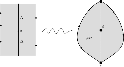
Figure 16. The unfolding of $\mathbf{M}^{1}:\hom_{\mathcal{W}^{2}}(\Delta,\Delta)\rightarrow\hom_{\mathcal{W}\mathrm{\!-\!mod\!-\!}\mathcal{W}}(\mathbf{M}(\Delta),\mathbf{M}(\Delta))$ to give the glued pair of discs corresponding to ${{}_{2}}\mathcal{CO}$.

Thus, as Proposition 5.6 implies that ${{}_{2}\mathcal{CO}}$ is homotopic to $\mathcal{CO}$, we see that an isomorphism

(9.28) $$SH^{*}(M)\stackrel{{\scriptstyle\mathcal{CO}}}{{\longrightarrow}}\mathrm{HH}^{*}(\mathcal{W},\mathcal{W})$$

is implied by the statement that $\mathbf{M}$ is full on $\Delta$. In turn, this statement may be reduced by the following proposition to showing that in the category $\mathcal{W}^{2}$, $\Delta$ is split-generated by objects of the form $L_{i}\times L_{j}$.

10. Forgotten points and homotopy units

In this section, we introduce an important technical tool used in our result: homotopy units for glued pairs of discs. We can motivate the need and/or application of such a tool as follows:

Suppose for a moment that we are in an idealized setting of Lagrangian Floer theory for a single Lagrangian $L\subset M$, in which we may ignore all issues of perturbations, transversality of moduli spaces, and obstructedness of Floer groups. Let us also for a moment reason using the conceptually intuitive singular chain variant of Floer theory as developed by [Fukaya:2009ve]. In this framework, generators of the Floer chain complex $CF(L,L)$ are given by equivalence classes of geometric (singular) cycles in $L$. Given cycles $\mathfrak{b}_{1},\ldots,\mathfrak{b}_{k}$, we define the $A_{\infty}$ structure map $\mu^{k}$ to be:

(10.1) $$\mu^{k}(\mathfrak{b}_{k},\ldots,\mathfrak{b}_{1}):=(ev_{0})_{*}[\mathcal{M}^{k}(\mathfrak{b}_{k},\ldots,\mathfrak{b}_{1})]$$

Here $[\mathcal{M}^{k}(\mathfrak{b}_{k},\ldots,\mathfrak{b}_{1})]$ is a “virtual fundamental chain” for the moduli space of holomorphic maps

$$u:(D,\partial D,z_{1}^{+},\ldots,z_{k}^{+},z_{0}^{-})\rightarrow(M,L,\mathfrak{b}_{1},\ldots,\mathfrak{b}_{k},\cdot)$$

with positive boundary marked points $z_{i}^{+}$ constrained to lie on the cycles $\mathfrak{b}_{i}$, and negative boundary marked point $z_{0}$ unconstrained. The notation from (10.1) simply means that we take as result the cycle “swept out” by the marked point $z_{0}^{-}$ in this moduli space.

In this (unfortunately imaginary) setting, there is a canonical choice of strict unit for the $A_{\infty}$ algebra $CF(L,L)$: the fundamental class $[L]$. This cycle satisfies the fundamental property that for $u:(D,\partial D)\rightarrow(M,L)$, the condition that $z_{i}\in\partial D$ lies on the cycle $[L]$ is an empty constraint.

Let us very informally show that this property gives $[L]$ the structure of a strict unit. First, work in the stable range $d\geq 3$. There is a projection map

(10.2) $$\pi_{j}:\mathcal{R}^{d}\rightarrow\mathcal{R}^{d-1},$$

forgetting the $j$th marked point. In the above setting, $\pi_{j}$ extends to a map between moduli spaces of stable maps:

(10.3) $$(\pi_{j})_{*}:\mathcal{M}^{d}(\mathfrak{b}_{1},\ldots,\mathfrak{b}_{k})\rightarrow\mathcal{M}^{d-1}(\mathfrak{b}_{1},\ldots,\mathfrak{b}_{j-1},\mathfrak{b}_{j+1},\ldots,\mathfrak{b}_{k})$$

Suppose $\mathfrak{b}_{j}=[L]$, an empty constraint on the marked point $z_{j}$. This implies that $(\pi_{j})_{*}$ is a submersion with one-dimensional fibers, corresponding to the location of the $j$th marked point. In particular,

$$\dim\mathcal{M}^{d}(\mathfrak{b}_{1},\ldots,\mathfrak{b}_{k})=\dim\mathcal{M}^{d-1}(\mathfrak{b}_{1},\ldots,\mathfrak{b}_{j-1},\ldots,\mathfrak{b}_{j+1},\ldots,\mathfrak{b}_{k})+1,$$

which implies that $(ev_{0})_{*}\mathcal{M}^{d}(\mathfrak{b}_{1},\ldots,\mathfrak{b}_{k})$ is a degenerate chain and thus zero on homology. Hence

(10.4) $$\mu^{d}(\ldots,[L],\ldots)=0.$$

When $d=2$, we leave it as a pictorial exercise to the interested reader to “prove” that

$$\mu^{2}([L],x)=\pm\mu^{2}(x,[L])=\pm x.$$

Even in this setting, there are a number of issues:

• in order to obtain transversality, one needs to coherently perturb the holomorphic curve equations in a domain-dependent manner and there is no known way to make the forgetful map compatible with these perturbations. These perturbations occur in the setting of Kuranishi structures, making them even less likely to be compatible with the forgetful map.

• strictly speaking, this moral argument only proved the equality (10.4) modulo degenerate chains. To move to an $A_{\infty}$ structure on $H^{*}(L)$, a host of additional arguments are required, including homological perturbation theory. The pay-off is that after some additional work one obtains a strictly unital structure on $H^{*}(L)$.

The reader is referred to [Fukaya:2009qf]*Ch. 7, §31 for details on Fukaya-Oh-Ohta-Ono’s approach to these problems.

In our setting, generators are time-1 Hamiltonian chords, so we have an additional issue:

• even if transversality were not an issue, we have no time-1 chord(s) $x$ with the property that imposing an asymptotic condition to $x$ is a forgetful map.

The remedy that seems to have been used in the literature most is this: construct a homology level unit geometrically, and then apply algebraic results of Seidel to obtain a quasi-isomorphic $A_{\infty}$ algebra that is strictly unital.

However, we are in a setting where we do not just care about algebraic properties of strictly unital $A_{\infty}$ categories. We would like to carefully analyze certain operations on $\mathcal{W}^{2}$ controlled by forgetful maps applied to submanifolds of moduli spaces of open-closed surfaces and pairs of discs. To be able to use such operations in $\mathcal{W}^{2}$, we will need them to be homotopic to existing operations.

If the reader wished to skip most of this section, the eventual punchline is this: Given some operations controlled by a submanifold $\mathcal{Q}$ of open-closed strings, the construction of homotopy units gives us a quasi-isomorphic category with additional elements $e^{+}_{j}\in\chi(L_{j},L_{j})$ such that the operation $\mathcal{Q}(\cdots e^{+}_{j}\cdots)$ is controlled by the submanifold $\pi_{j}(\mathcal{Q})$.

10.1. Forgotten marked points

We begin with a notion of what it means to have forgotten a boundary marked point in Floer-theoretic operations. Since the construction is identical for discs and pairs of glued discs, we initiate them in parallel. Strictly speaking, we do not need the single-disc construction in our paper, but it is no additional work and may be foundationally useful. Also, we only consider forgotten points on pairs of identical discs modulo simultaneous automorphism, the only case that arises for us.

Definition 10.1.

The moduli space of discs with $d$ marked points and $F\subseteq\{1,\ldots,d\}$ forgotten marked points, denoted

(10.5) $$\mathcal{R}^{d,F}$$

is exactly the moduli space of discs $\mathcal{R}^{d}$ with marked points labeled as belonging to $F$.

Definition 10.2.

The moduli space of $\mathfrak{S}$-glued pairs of discs with $(k,l)$ marked points, $\mathfrak{T}$ point identifications, and

(10.6) $$(F_{1},F_{2})\subseteq(\{1,\ldots,k\},\{1,\ldots,l\}),$$

forgotten points, denoted

(10.7) $${}_{\mathfrak{S},\mathfrak{T}}\mathcal{R}_{k,l}^{(F_{1},F_{2})}$$

is the image of the diagonal associahedron in the moduli space of glued pairs of discs $\mathcal{R}_{k,k,\mathfrak{S}}$ with positive marked points on each disc corresponding to $F_{1}$ and $F_{2}$ labeled as forgotten points. Crucially, $F_{1}$ and $F_{2}$ must satisfy the following conditions:

• $F_{1}$ and $F_{2}$ are subsets of the left and right identified points respectively. Namely,

  (10.8) $$F_{i}\subset\pi_{i}(\mathfrak{T}),$$

  where $\pi_{i}$ is projection onto the $i$th component.

• $F_{1}$ and $F_{2}$ are not associated to a boundary identification, i.e.

  (10.9) $$F_{i}\cap\pi_{i}(p(\mathfrak{S}))=\emptyset$$

• $F_{1}$ and $F_{2}$ do not contain both the left and right points of any identification, i.e.

  (10.10) $$(F_{1}\times F_{2})\cap\mathfrak{T}=\emptyset$$

Remark 10.1.

Put another way, the conditions $F_{1}$ and $F_{2}$ must satisfy correspond to the following from the viewpoint of tricolored discs developed in Section 7: $F_{1}$ and $F_{2}$ correspond to disjoint subsets of the points colored $LR$, such that neither $F_{1}$ or $F_{2}$ is adjacent to a boundary component labeled as identified.

For the purpose of solving Floer’s equations, we will be putting the marked points labeled by $F$, $F_{i}$ back in. Such points should be thought of as markers rather than punctures.

Definition 10.3.

Let $I\subseteq F$. The $I$-forgetful map

(10.11) $$\mathcal{F}_{I}:\mathcal{R}^{d,F}\longrightarrow\mathcal{R}^{d-|I|,F^{\prime}}$$

associates to any $S$ the surface obtained by putting the points of $I$ back in and forgetting them. $F^{\prime}$ in the equation above is the set of forgetful points $F-I$, re-indexed appropriately.

There is a similar forgetful map for pairs of glued discs,

(10.12) $$\mathcal{F}_{I_{1},I_{2}}:_{\mathfrak{S},\mathfrak{T}}\mathcal{R}_{k,l}^{F_{1},F_{2}}\longrightarrow_{\mathfrak{S}^{\prime},\mathfrak{T}^{\prime}}\mathcal{R}_{k-|I_{1}|,l-|I_{2}|}^{F_{1}^{\prime},F_{2}^{\prime}}$$

We need a notion that corresponds to stability of the underlying disc once we have forgotten points.

Definition 10.4.

A disc with $d$ marked points and $F$ forgotten points is f-stable or f-semistable if $d-|F|\geq 2$ or $d-|F|=1$ respectively. A pair of discs with $(k,l)$ marked points and $F_{1},F_{2}$ forgotten points is f-stable if $k-|F_{1}|$, $l-|F_{2}|$ are both greater than or equal to 1 and one is greater than or equal to 2. It is f-semistable if both of these quantities are equal to 1.

In the f-stable range, there are maximally forgetful maps, collectively denoted $\mathcal{F}_{max}$:

(10.13) $$\mathcal{F}_{max}=\mathcal{F}_{F}:\mathcal{R}^{d,F} \longrightarrow\mathcal{R}^{d-|F|}$$

(10.14) $$\mathcal{F}_{max}=\mathcal{F}_{F_{1},F_{2}}:{{}_{\mathfrak{S},\mathfrak{T}}}\mathcal{R}_{k,l}^{F_{1},F_{2}} \longrightarrow_{\mathfrak{S}^{\prime},\mathfrak{T}^{\prime}}\mathcal{R}_{k-|F_{1}|,l-|F_{2}|}\$$

The (Deligne-Mumford) compactifications

(10.15) $$\overline{\mathcal{R}}^{d,F}$$

(10.16) $${}_{\mathfrak{S},\mathfrak{T}}\overline{\mathcal{R}}_{k,l}^{F_{1},F_{2}}$$

are exactly the usual Deligne-Mumford compactifications, along with the data of forgotten labels for the relevant boundary marked points. Interior positive nodes inherit the label of forgotten in the following fashion:

Definition 10.5.

An interior positive node of a stable representative $S$ of a disc or pair of glued discs is said to be a forgotten node if and only if every boundary marked point in every component above $p$ is a forgotten marked point and there are no interior marked points in any component above $p$.

In the $f$-stable range, stable discs with forgotten marked points have underlying stable representatives with forgotten points removed.

Definition 10.6.

A component of a stable representative $S$ of a disc or a pair of glued discs is said to be forgettable if all of its positive boundary marked points (including nodal ones) are forgotten points and it has no interior marked points.

Using the above definitions, one can extend the maximally forgetful map to compactifications.

Definition 10.7.

Let $S$ be a nodal bordered f-stable surface with forgotten marked points. The associated reduced surface $\hat{S}$ is the nodal surface obtained by

• eliminating all forgettable components

• putting back in all forgotten boundary points and forgetting them

• if in the $f$-stable range, eliminating any non-main component with only one non-forgotten marked point $p$, and labeling the positive marked point below this component by $p$.

Define the induced marked points of $\hat{S}$ to be the boundary marked points that survive this procedure.

In other words, the nodal surface $\hat{S}$ is obtained from the nodal surface $S$ by forgetting the points with an $F$ label and then stabilizing the resulting bubble tree.

Definition 10.8.

The maximally forgetful map $\mathcal{F}_{max}$, defined for any nodal $f$-semistable disc or pair of glued discs is defined to be the map that associate to a nodal surface with forgotten marked points $S$ the associated reduced surface $\hat{S}$.

Definition 10.9.

A Floer datum for a stable, $f$-semistable disc or pair of glued discs with forgotten marked points consists of a Floer datum for the associated reduced surface $\hat{S}=\mathcal{F}_{max}(S)$, in the sense of Definition 4.11 or Definition 7.16, satisfying the following conditions:

• in the f-stable range, it is identical to our previously chosen Floer datum for $\hat{S}$ thought of as an open-closed string.

• in the f-semistable range, it is given by the unique translation-invariant Floer datum on the strip $\hat{S}$.

This implies in particular that the Floer datum only depends on the point $\mathfrak{F}_{max}(S)$.

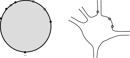
Figure 17. Two drawings of a disc with forgotten points (denoted by hollow points). The drawing on the right emphasizes the choice of strip-like ends.

Remark 10.2.

By the above definition, a Floer datum for a pair of discs $P$ with $\mathfrak{S}$ boundary identifications, $\mathfrak{T}$ point identifications, and $F_{1},F_{2}$ forgotten points is a Floer datum for the open-closed string obtained by forgetting the marked points corresponding to $F_{1}$ and $F_{2}$, stabilizing, and gluing the resulting pairs of discs via $\pi_{\mathfrak{S}}$.

Because we have chosen our Floer data to be the one we have already chosen for the underlying reduced open-closed string, we immediately obtain:

Proposition 10.1.

There exists a universal and consistent choice of Floer data for discs or pairs of glued discs with forgotten marked points.

Definition 10.10.

An admissible Lagrangian labeling for a surface $S$ with forgotten marked points is a choice of Lagrangian labeling that descends to a well-defined labeling on the associated reduced surface $\mathcal{F}_{max}(S)$. Namely, if $p$ is any forgotten boundary marked point of $S$, then the labels before and after $p$ must coincide. The reduced labeling is the corresponding labeling on the underlying reduced surface.

Now, suppose we have fixed a universal and consistent choice of Floer data for discs. Consider a compact submanifold with corners of dimension $d$

(10.17) $$\overline{\mathcal{Z}}^{d}\lhook\joinrel\relbar\joinrel\rightarrow{{}_{\mathfrak{S},\mathfrak{T}}}\mathcal{R}_{k,l}^{F_{1},F_{2}}.$$

with an admissible Lagrangian labeling $\vec{L}$. In the usual fashion, fix input and output chords $\vec{x}_{in},\vec{x}_{out}$ and orbits $\vec{y}_{in},\vec{y}_{out}$ for the induced marked points of the gluing $\pi_{\mathfrak{S}}(\mathcal{F}_{max}(\overline{\mathcal{Z}}^{d}))$, which forgets all points labeled as forgotten and glues along the boundary components $\mathfrak{S}$. Define

(10.18) $$\overline{\mathcal{Z}}^{d}(\vec{x}_{out},\vec{y}_{out};\vec{x}_{in},\vec{y}_{in})$$

to be the space of maps

(10.19) $$\{u:\pi_{\mathfrak{S}}(\mathcal{F}_{max}(S))\longrightarrow M:S\in\overline{\mathcal{Z}}^{d}\}$$

satisfying Floer’s equation with respect to the Floer datum and asymptotic and boundary conditions specified by the Lagrangian labeling $\vec{L}$ and asymptotic conditions $(\vec{x}_{out},\vec{y}_{out},\vec{x}_{in},\vec{y}_{in})$.

As before, $h(\mathfrak{S},k,l)$ denote the number of boundary components of any resulting surface obtained from the gluing.

Lemma 10.1.

The moduli spaces $\overline{\mathcal{Z}}^{d}(\vec{x}_{out},\vec{y}_{out};\vec{x}_{in},\vec{y}_{in})$ are compact, and empty for all but finitely many $(\vec{x}_{out},\vec{y}_{out})$ given fixed inputs $(\vec{x}_{in},\vec{y}_{in})$. For generically chosen Floer data, they form smooth manifolds of dimension

(10.20) $$\begin{split}\dim\overline{\mathcal{Z}}^{d}(\vec{x}_{out},\vec{y}_{out};\vec{x}_{in},\vec{y}_{in}):=\sum_{x_{-}\in\vec{x}_{out}}\deg(x_{-})+&\sum_{y_{-}\in\vec{y}_{out}}\deg(y_{-})\\ +(2-h(\mathfrak{S},k,l)-|\vec{x}_{out}|-2|\vec{y}_{out}|)n&+d-\sum_{x_{+}\in\vec{x}_{int}}\deg(x_{+})-\sum_{y_{+}\in\vec{y}_{in}}\deg(y_{+}).\end{split}$$

In the usual fashion, when the dimension of the spaces $\overline{\mathcal{Z}}^{d}(\vec{x}_{out},\vec{y}_{out};\vec{x}_{in},\vec{y}_{in})$ are zero, we can use natural isomorphisms of orientation lines to count (with signs) the number of points in such spaces, and associate operations

(10.21) $$(-1)^{\vec{t}}\mathbf{H}_{\overline{\mathcal{Z}}^{d}}$$

from the tensor product of wrapped Floer complexes and symplectic cochain complexes where $\vec{x}_{in}$, $\vec{y}_{in}$ reside to the tensor product of the complexes where $\vec{x}_{out}$, $\vec{y}_{out}$ reside. We can specify certain submanifolds of the space of forgotten marked points by applying forgotten labels to various boundary points on spaces of open-closed strings.

Definition 10.11.

The forget map

(10.22) $$\mathfrak{f}_{F}:\mathcal{R}^{d} \longrightarrow\mathcal{R}^{d,F}$$

(10.23) $$\mathfrak{f}_{F_{1},F_{2}}:{{}_{\mathfrak{S},\mathfrak{T}}}\mathcal{R}_{k,l} \longrightarrow{{}_{\mathfrak{S},\mathfrak{T}}}\mathcal{R}_{k,l}^{F_{1},F_{2}}$$

simply marks boundary points with indices in $F$ (or $(F_{1},F_{2})$) as forgotten.

10.2. Operations with forgotten points

Our main application is of course to think of forgotten points as formal units, either for a disc or pair of discs. It is thus illustrative to see how operations with forgotten marked points either vanish or reduce to other known operations.

Proposition 10.2.

Let $F\subset\{1,\ldots,d\}$ be a non-empty subset of size $0<|F|<d$. Then the operation associated to $\overline{\mathcal{R}}^{d,F}$ is zero if $d>2$ and the identity operation $I(\cdot)$ (up to a sign) when $d=2$.

Proof.

Suppose first that $d>2$, and let $u$ be any solution to Floer’s equation over the space $\mathcal{R}^{d,F}$ with domain $S$. Let $p\in F$ be the last element of $F$. Since the Floer data on $S$ only depends on $\mathcal{F}_{p}(S)$, we see that maps from $S^{\prime}$ with $S^{\prime}\in\mathcal{F}_{p}^{-1}(\mathcal{F}_{p}(S))$ also give solutions to Floer’s equation with the same asymptotics. Moreover, the fibers of the map $\mathcal{F}_{p}$ are one-dimensional, implying that $u$ cannot be rigid, and thus the associated operation is zero.

Now suppose that $d=2$, and without loss of generality $F=\{1\}$. Then the forgetful map associates to the single point $[S]\in\mathcal{R}^{2,F}$ the unstable strip with its translation invariant Floer datum. We conclude, based on Section 6.1, that the resulting operation is the identity. ∎

Remark 10.3.

Actually, one would like this operation to be zero when $|F|=d$ as well. However, we have not defined an operation with $|F|=d$, due to the instability of the underlying reduced surface. Our solution will be to declare this operation to be zero, and check that our declaration is compatible with the behavior of boundaries of one dimensional moduli spaces.

Proposition 10.3.

Let $\Delta_{d}\subset\mathcal{R}_{d,d}$ be the diagonal associahedron. Let $[d]$ denote the set $\{1,\ldots,d\}$, and $(k,l)$ such that pairs of discs with $k$,$l$ marked points are stable. Then, the operation given by the disjoint union

(10.24) $$\coprod_{I\subset[k+l]||I|=k}(\mathfrak{f}_{I,[k+l]-I})(\Delta_{k+l})$$

with appropriate orientations is identical to the operation given by $\mathcal{R}_{k,l}$. In other words, it is equal to zero when $k$, $l$ $\geq 1$ and one is $\geq 2$.

Proof.

On the open locus ${}_{0}\mathcal{R}_{k,l}$ where none of the $k$ points on the first disc and the $l$ points on the second disc are in identical positions, we can consider the overlay map:

(10.25) $${}_{0}\mathcal{R}_{k,l}\longrightarrow\coprod_{I\subset[k+l]||I|=k}(\mathfrak{f}_{I,[k+l]-I})(\Delta_{k+l}(\mathcal{R}^{k+1}))$$

given by marking the $l$ positive marked points on $S_{2}$ as extra forgotten points on $S_{1}$ and vice versa. On the level of tricolored discs, the overlay makes $L$ points $LR$ points with the $R$ component marked as forgotten, and makes $R$ points $LR$ points with the $L$ component marked as forgotten. By construction, this map is compatible with Floer data, and covers the entire interior of the target. Since after a perturbation zero-dimensional solutions to Floer’s equation come from a representative on the interior of any source abstract moduli space, we conclude that the two operations in the Proposition are identical, modulo sign. See Figure 18 for an example of this overlay map. ∎

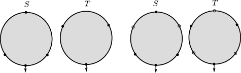
Figure 18. An example of the overlay map from ${}_{0}\mathcal{R}_{3,2}$ to $\mathcal{R}_{5,5}^{\{2,4\},\{1,3,5\}}$.

Proposition 10.4.

Take boundary identification $\mathfrak{S}=\{(1,1)\}$ and maximal point identification $\mathfrak{T}_{max}=\{(1,1),\ldots,(k+l,k+l)\}$. Then, letting $S=\{2,\ldots,k+l-2\}$, the operation corresponding to

(10.26) $$\coprod_{I\subset S||I|=k-1}\mathfrak{f}_{I,S-I}({{}_{\mathfrak{S},\mathfrak{T}_{max}}}\mathcal{R}_{k,l})$$

is $\mu^{k+l-1}$ (with suitable sign twisting datum).

Proof.

On the open locus of ${}_{(1,1),(1,1)}\mathcal{R}_{k,l}$ where the only coincident points are $(1,1)$ and no other points coincide, denoted

(10.27) $${}_{(1,1),(1,1)}\mathcal{R}_{k,l}^{0}$$

there is once more an overlay map

(10.28) $${}_{(1,1),(1,1)}\mathcal{R}_{k,l}^{0}\longrightarrow\coprod_{I\subset S||I|=k-1}\mathfrak{f}_{I,S-I}({{}_{\mathfrak{S},\mathfrak{T}_{max}}}\mathcal{R}_{k,l})$$

given by superimposing left and right discs, and marking points from the right as forgotten points on the left and vice versa. This gives an isomorphism of spaces with Floer data on the open locus, so we conclude by applying Proposition 7.7 to calculate the operation associated to ${}_{(1,1),(1,1)}\mathcal{R}_{k,l}$. ∎

Proposition 10.5.

Take boundary identification $\mathfrak{S}=\{(k+l,k+l)\}$ and maximal point identification $\mathfrak{T}_{max}=\{(1,1),\ldots,(k+l,k+l)\}$. Then, letting $S=\{1,\ldots,k+l-1\}$, the operation corresponding to

(10.29) $$\coprod_{I\subset S||I|=k-1}\mathfrak{f}_{I,S-I}({{}_{\mathfrak{S},\mathfrak{T}_{max}}}\mathcal{R}_{k,l})$$

is $\mu^{k+l-1}$ (with suitable sign twisting datum).

Proof.

The proof is identical to the above case, using an overlay map and reducing to Proposition 7.7. ∎

Proposition 10.6.

Take boundary identification $\mathfrak{S}=\{(1,1),(k+l,k+l)\}$ and maximal point identification $\mathfrak{T}_{max}=\{(1,1),\ldots,(k+l,k+l)\}$. Then, letting $S=\{2,\ldots,k+l-1\}$, the operation corresponding to

(10.30) $$\coprod_{I\subset S||I|=k-2}\mathfrak{f}_{I,S-I}({{}_{\mathfrak{S},\mathfrak{T}_{max}}}\mathcal{R}_{k,l})$$

is ${}_{2}\mathcal{OC}^{k-2,l-2}$ (with suitable sign twisting datum).

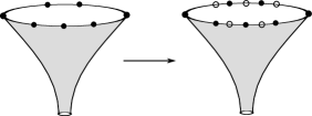
Figure 19. The overlay map from ${}_{\mathfrak{S},p(\mathfrak{S})}\mathcal{R}_{5,4}$ to ${}_{\mathfrak{S}^{\prime},p(\mathfrak{S})^{\prime}}\mathcal{R}_{7,7}^{\{3,5\},\{2,4,6\}}$, where $\mathfrak{S}=\{(1,1),(5,4)\}$ and $\mathfrak{S^{\prime}}=\{(1,1),(7,7)\}$. Forgotten points are marked with rings.

Proof.

The same arguments using overlay maps as before apply, only now we compare to ${}_{\{(1,1),(k,l)\},\{(1,1),(k,l)\}}\mathcal{R}_{k,l}$. The associated operation is, by Proposition 7.8, ${}_{2}\mathcal{OC}^{k-2,l-2}$. See Figure 19 for an example of this particular overlay map. ∎

10.3. A local model

Our definition of forgetful operations and homotopy units is based upon the following local model. Let ${\mathbb{H}}$ denote the upper half plane and ${\mathbb{H}}^{o}$ the upper half plane with the origin removed. Viewing ${\mathbb{H}}$ as a disc with a point removed, and ${\mathbb{H}}^{o}$ as a disc with two points removed, there is the natural “forgetful” map

(10.31) $$F:{\mathbb{H}}^{o}\lhook\joinrel\relbar\joinrel\rightarrow{\mathbb{H}}$$

which forgets the special point 0. Consider the following negative strip-like end around $\infty$:

(10.32) $$\epsilon_{\mathbb{H}}:(-\infty,0]\times[0,1] \longrightarrow{\mathbb{H}}$$

(10.33) $$(s,t) \longmapsto\exp(-\pi(s+it))$$

which has image $\{(r,\theta)|r\geq 1\}\subset{\mathbb{H}}$. For ${\mathbb{H}}^{o}$, define the following basic positive strip-like end around 0:

(10.34) $$\epsilon_{{\mathbb{H}}^{o}}:[0,\infty)\times[0,1] \longrightarrow{\mathbb{H}}^{0}$$

(10.35) $$(s,t) \longmapsto 2\cdot\exp(-\pi(s+it)).$$

This end has image $\{(r,\theta)|0<r\leq 2\}\subset{\mathbb{H}}^{o}.$ With these special choices of strip-like ends, we observe that 0-connect sum is exactly the forgetful map $F$. The precise statement is this:

Proposition 10.7.

Let ${\mathbb{T}}$ be the associated thick part in ${\mathbb{H}}^{0}$ of the 0 connect sum

$$C:={\mathbb{H}}^{o}\#^{0}_{(\epsilon_{{\mathbb{H}}^{o}},0),(\epsilon_{\mathbb{H}},\infty)}{\mathbb{H}}$$

and let $C^{0}$ denote the complement of $0\in{\mathbb{H}}$ in the connect sum $C$. Then, there is a commutative diagram

(10.36)

Proof.

This is obvious via viewing each of these regions and the connect sum itself as subsets of ${\mathbb{H}}$. ∎

10.4. Revisiting the unit

We revisit our choice of Floer datum for the explicit geometric unit map, defined in Section 6.2. Let $\Sigma_{0}={\mathbb{H}}$ once more denote the upper half plane, and fix an outgoing striplike end at $\infty$ given by $\epsilon_{{\mathbb{H}}}$, defined in (10.32).

Let $\psi:[0,\infty)\longrightarrow[0,1]$ be a smooth function equaling 0 in a neighborhood of 0 and 1 in a neighborhood of $[1,\infty)$.

Given a weight $w=1$, and a Hamiltonian $H$, fix the following Floer datum on ${\mathbb{H}}$:

• one form $\alpha_{{\mathbb{H}}}$ given by $-\frac{1}{\pi}\cdot\psi(r)d\theta$

• rescaling function $a_{{\mathbb{H}}}$ equal to 1.

• any primary Hamiltonian, $H_{\mathbb{H}}$ that is compatible with the strip-like end $\epsilon_{\mathbb{H}}$

• any almost complex structure that is compatible with $\epsilon_{\mathbb{H}}$.

• some constant perturbation term $F_{\mathbb{H}}$.

Define the Floer datum for arbitrary weight $w$ to be the $w$ conformal rescaling of the above Floer datum. It has the following properties:

• one form $\alpha_{{\mathbb{H}}}^{w}$ given by $-\frac{1}{\pi}\cdot w\psi(r)d\theta$

• rescaling function $a_{{\mathbb{H}}}^{w}$ equal to $w$.

• primary Hamiltonian $H_{{\mathbb{H}}}^{w}$ given by $\frac{H_{\mathbb{H}}\circ\psi^{w}}{w^{2}}$

• almost complex structure $J_{{\mathbb{H}}}^{w}$ given by $(\psi^{w})^{*}J_{\mathbb{H}}$

• perturbation term $F_{\mathbb{H}}^{w}$ given by $w\cdot F_{\mathbb{H}}$, another constant.

Call the above datum a standard unit datum of type $w$. By design, $\epsilon_{{\mathbb{H}}}^{*}(\alpha_{{\mathbb{H}}}^{w})=wdt$.

10.5. Damped connect sums

We describe a local model, depending on a time parameter

(10.37) $$\tau\in[0,1],$$

that gives a homotopy relating a “formal unit,” or forgotten marked point, to the geometric unit described in Section 6 and again above. We would like such a homotopy, which we call a $\tau$-damped connect sum, to have the following properties in a neighborhood of a given forgotten point $p$ on a surface $S$.

• at time $\tau=0$, the Floer datum is essentially unconstrained in a neighborhood of $p$, agreeing with whatever Floer datum we obtained by forgetting $p$ and compactifying.

• at intermediate time $\tau$, the Floer datum is modeled on a growing connect sum of a neighborhood of $p$ with a disc with one output, thought of as ${\mathbb{H}}$ with output at $\infty$.

• the $\tau=1$ limit is the nodal connect sum ${\mathbb{H}}\#^{1}_{p}S$. The Floer datum on the ${\mathbb{H}}$ component should agree with the Floer datum on the geometric unit, and the Floer data on the $p$ side should agree with a standard, previously chosen Floer datum.

Readers who wish to skip this section should treat the $\tau$-damped connect sum along a boundary point $p$ as a formal operation on surfaces with Floer data, satisfying the property that at $\tau=0$, one has the forgetful map, and at $\tau=1$, one has nodally glued on an ${\mathbb{H}}$.

In reality, we will need to construct such an operation in two steps:

• for $\tau\in(0,\frac{1}{2})$, the Floer datum on $S$ goes from arbitrary with respect to $p$ to (partially) compatible with respect to a strip-like end around $p$.

• for $\tau\in(\frac{1}{2},1)$, the datum is modeled as a growing connect sum as before.

Figure 20. A schematic of a damped connect sum (though in reality, the conformal structure of $S$ will stay the same).

The basic setup is as follows: Let $S$ be a Riemann surface with boundary, with some boundary marked points removed. Fix one such positive boundary marked point $z$, with strip-like end around $z$

(10.38) $$\epsilon_{z}:[0,\infty)\times[0,1]\longrightarrow S.$$

Definition 10.12.

Let $\hat{S}_{z}$ be $S$ with the point $z$ filled back in. Call the strip-like end $\epsilon_{z}$ rational if it extends to a holomorphic map $\bar{\epsilon}_{z}:([0,1]\times[0,\infty))\cup\{\infty\}\longrightarrow\hat{S}_{z}$.

Remark 10.4.

Working with rational strip-like ends does not impose any additional trouble in choosing Floer data. We can implicitly choose all of our strip-like ends $\epsilon:Z_{+}\rightarrow S$ to be rational. See e.g. [Abouzaid:2010ly]*Addendum 2.3.

Now, let $\epsilon_{z}$ be any rational striplike end. Let $D_{2}^{0}$ denote the punctured upper half radius two disc $\{0<|z|\leq 2\}\subset{\mathbb{C}}$ and $D_{2}$ the domain arising from $D_{2}^{0}$ by filling in the origin, i.e. $D_{2}=\{0\leq|z|\leq 2\}$. By precomposing with the standard map

(10.39) $$\begin{split}\epsilon_{{\mathbb{H}}_{0}}^{-1}:D_{2}^{0}&\longrightarrow[0,\infty)\times[0,1]\\ z&\longmapsto(\ln(\frac{2}{|z|}),1-\frac{\arg(z)}{\pi})\end{split}$$

we may equivalently suppose $\epsilon_{z}$ is a map $\tilde{\epsilon}_{z}$ from $D_{1}^{0}$ to $S$ that extends to a map from $D_{2}$ to $\hat{S}_{z}$. Call $\tilde{\epsilon}_{z}$ the associated disc-like end of $\epsilon_{z}$, and let $\bar{\tilde{\epsilon}}_{z}$ be the associated map from $D_{2}$ to $\hat{S}_{z}$.

Now, fix a time-parameter $\tau\in[0,1]$. In a manner depending on $\tau$, we weaken the notion of compatibility with respect to the strip-like end $\epsilon_{z}$.

Definition 10.13.

A Floer datum ($\alpha_{S}$, $a_{S}$, $J_{S}$, $H_{S}$, $F_{S}$) is said to be $\tau$-partially compatible with a strip-like end $(z,\epsilon)$, for $\tau\in[0,1]$, if the datum extends to one on the compactification $\hat{S}_{z}$ when $\tau\in[0,\frac{1}{2}]$ and the conditions

(10.40) $$\begin{split}\epsilon^{*}a_{S}&=w_{1}(\tau)\\ \epsilon^{*}\alpha_{S}&=w_{2}(\tau)dt\\ \epsilon^{*}H_{S}&=\frac{H\circ\psi^{w_{2}(\tau)}}{w_{2}(\tau)^{2}}\end{split}$$

hold when $\tau\geq\frac{1}{2}$. Furthermore, we require that at $\tau=1$, $\tau$-compatibility is genuine compatibility; in other words,

(10.41) $$w_{1}(1)=w_{2}(1).$$

Remark 10.5.

In the limit $\tau=0$, $\tau$-partial compatibility is an empty condition for the Floer data on $S$. Note that in contrast to normal Floer data, we are using two potentially different functions $w_{1}(\tau)$ and $w_{2}(\tau)$. In other words, we are not requiring the value of the one-form $\alpha_{S}$ or the amount flowed by the Hamiltonian to always be the same as the amount of rescaling or time-shifting performed by the almost complex structure or Lagrangian boundary. This is sensible—on a boundary point that is not a priori a striplike end, the one form $\alpha_{S}$ is asymptotically 0, but $a_{S}$ is always non-zero.

Definition 10.14.

Let $S$ have rational strip-like end $\epsilon_{z}$ around $z$ with associated disc-like end $\tilde{\epsilon}_{z}$, and suppose we have chosen a Floer datum $\mathbf{D}^{\tau}$ that is $\tau$-compatible with $\tilde{\epsilon}_{z}$. An associated $\tau$-structure on ${\mathbb{H}}$, denoted $\mathbf{D}_{{\mathbb{H}}}^{\tau}(z)$ consists of the following Floer datum on ${\mathbb{H}}$, depending on $\tau$:

• for $\tau\in[0,\frac{1}{2}]$, the Floer datum $\mathbf{D}$ extends to the compactification $\hat{S}_{z}$. The pullback $(\bar{\tilde{e}}_{z})^{*}D$ gives some Floer datum on $D_{2}$. Define the Floer datum on ${\mathbb{H}}$ to be any datum extending this one to all of ${\mathbb{H}}$.

• For $\tau\in[\frac{1}{2},1]$, the Floer datum is defined as follows:

  • one-form $\alpha_{\mathbb{H}}^{\tau}(\mathbf{D})$ given by $-\frac{1}{\pi}w_{2}(\tau)\cdot\psi(r)d\theta$.

  • any primary Hamiltonian $H^{\tau}(\mathbf{D})$ equal to $\frac{H\circ\psi^{w_{2}(\tau)}}{w_{2}(\tau)^{2}}$ on the striplike end $\epsilon_{\mathbb{H}}$.

  • any rescaling function $a_{S}^{\tau}(\mathbf{D})$ equal to $w_{1}(\tau)$ when restricted to $\epsilon_{\mathbb{H}}$.

  • any complex structure equal to $(\psi^{a_{S}^{\tau}(\mathbf{D})})^{*}J_{t}$ on $\epsilon_{\mathbb{H}}$.

Furthermore, we mandate that when $\tau=1$, the Floer datum on ${\mathbb{H}}$ must be the standard unit datum of type $w_{1}(1)=w_{2}(1)$.

Pick a smooth non-decreasing function $\kappa:[0,1]\longrightarrow[0,1]$ that is 0 in a neighborhood of $[0,\frac{1}{2}]$ and 1 exactly at 1.

Definition 10.15.

Let $S$ have rational strip-like end $\epsilon_{z}$ around $z$ with associated disc-like end $\tilde{\epsilon}_{z}$, and suppose we have chosen a Floer datum $\mathbf{D}^{\tau}$ that is $\tau$-compatible with $\tilde{\epsilon}_{z}$, and an associated $\tau$-structure on ${\mathbb{H}}$, $\mathbf{D}_{\mathbb{H}}^{\tau}(z)$. Define the $\tau$-damped connect sum

(10.42) $$S\sharp^{\tau}_{z}{\mathbb{H}},$$

to be the surface

(10.43) $$S\#^{\kappa(\tau)}_{z,\infty}{\mathbb{H}}$$

equipped with the Floer datum $\mathbf{D}^{\tau}$ on $S-\epsilon_{z}([0,\infty)\times[0,1])$ and the Floer datum $\mathbf{D}_{\mathbb{H}}^{\tau}(z)$ on ${\mathbb{H}}$ elsewhere.

By construction, this is a smooth Floer datum on $S\sharp^{\tau}_{z}{\mathbb{H}}$, and satisfies the following properties:

• For $\tau\in[0,\frac{1}{2}]$ it agrees with the compactified Floer datum $\hat{\mathbf{D}}^{\tau}$ on $\hat{S}_{z}$.

• For $\tau=1$, it is the nodal connect sum

  (10.44) $$S\#^{1}{\mathbb{H}}$$

  where ${\mathbb{H}}$ is equipped with the standard unit datum of type $w_{1}(\tau)=w_{2}(\tau)$, and $S$ has some Floer datum $\mathbf{D}^{1}$ that is genuinely compatible with $S,z,\epsilon_{z}$ in the usual sense.

Remark 10.6.

We should note that any intermediate damped connect sum with a copy of ${\mathbb{H}}$ for our choices of standard strip-like ends (10.32) is conformally equivalent to the forgetful map. All that changes as the damped connect sum parameter approaches 1 is that the standard unit Floer datum is rescaled and shrunk into a smaller and smaller neighborhood of the marked point, until eventually at time 1 it is forced to break off. Despite this, it is useful sometimes to visualize the process as a topological connect sum.

10.6. Abstract moduli spaces and operations

Definition 10.16.

The moduli space of discs with $d$ marked points, $F\subset[d]$ forgotten points, and $H\subset[d]-F$ homotopy units

(10.45) $$\mathfrak{H}^{d,F,H}$$

is exactly the moduli space of discs $\mathcal{R}^{d}$, with points in $F$ or $H$ labeled as belonging to $F$ or $H$ times a copy of $[0,1]$ for each element of $H$:

(10.46) $$\mathfrak{H}^{d,F,H}\simeq\mathcal{R}^{d}\times[0,1]^{|H|}.$$

When $H=\emptyset$, we define $\mathfrak{H}^{d,F,\emptyset}=\mathcal{R}^{d,F}$.

We think of a point in this moduli space as a pair $(S,\vec{v}=(v_{1},\ldots,v_{|H|}))$. We associate the $i$th copy of the interval to the $i$th ordered point in $H$ in the following sense: Suppose $H$ is ordered $\{p_{n_{1}},\ldots,p_{n_{|H|}}\}$ Then, for each element of $H$, there are endpoint maps

(10.47) $$\pi_{p_{n_{i}}}^{1}:\mathfrak{H}^{d,F,H}|_{v_{i}=1} \longrightarrow\mathfrak{H}^{d,F,H-\{p_{n_{i}}\}}$$

(10.48) $$\pi_{p_{n_{i}}}^{0}:\mathfrak{H}^{d,F,H}|_{v_{i}=0} \longrightarrow\mathfrak{H}^{d,F+\{p_{n_{i}}\},H-\{p_{n_{i}}\}}$$

defined as follows: given an element $(S,\vec{v})$ $\pi^{1}_{p_{n_{i}}}$ removes the label $H$ from the point $p_{n_{i}}$ in $S$, and projects $\vec{v}$ away from the $i$th component (which is 1). $\pi^{0}_{p_{n_{i}}}$ removes the label of $H$ but assigns the label of $F$ to $p_{n_{i}}$, and projects $\vec{v}$ away from the $i$th component (which is 0).

Definition 10.17.

The moduli space of $\mathfrak{S}$-glued pairs of discs with $(k,l)$ marked points, $\mathfrak{T}$ point identifications, $F_{1},F_{2}\subset([k],[l])$ forgotten points, and $H_{1},H_{2}\subset([k],[l])$ homotopy units, denoted

(10.49) $${}_{\mathfrak{S},\mathfrak{T}}\mathfrak{H}_{k,l}^{F_{1},F_{2},H_{1},H_{2}}$$

is exactly the moduli space ${}_{\mathfrak{S},\mathfrak{T}}\mathcal{R}_{k,l}$ with points in $F_{1},F_{2},H_{1},H_{2}$ labeled accordingly, times a copy of $[0,1]$ for each element of $H_{1}$ or $H_{2}$:

(10.50) $${}_{\mathfrak{S},\mathfrak{T}}\mathfrak{H}_{k,l}^{F_{1},F_{2},H_{1},H_{2}}\simeq_{\mathfrak{S},\mathfrak{T}}\mathcal{R}_{k,l}\times[0,1]^{|H_{1}|}\times[0,1]^{|H_{2}|}.$$

As with forgotten marked points, we have the following constraints:

• $F_{1},H_{1}$ and $F_{2},H_{2}$ are disjoint subsets of the left and right identified points respectively. Namely,

  (10.51) $$F_{i},H_{i}\subset\pi_{i}(\mathfrak{T}),F_{i}\cap H_{i}=\emptyset$$

  where $\pi_{i}$ is projection onto the $i$th component.

• $F_{1},H_{1}$ and $F_{2},H_{2}$ are not associated to a boundary identification, i.e.

  (10.52) $$(F_{i}\cup H_{i})\cap\pi_{i}(p(\mathfrak{S}))=\emptyset$$

• $F_{1},H_{1}$ and $F_{2},H_{2}$ do not contain both the left and right points of any identification, i.e.

  (10.53) $$((F_{1}\cup H_{1})\times(F_{2}\cup H_{2}))\cap\mathfrak{T}=\emptyset$$

We think of a point of ${}_{\mathfrak{S},\mathfrak{T}}\mathfrak{H}_{k,l}^{F_{1},F_{2},H_{1},H_{2}}$ as a tuple

(10.54) $$(P,\vec{v},\vec{w}).$$

Suppose $H_{1},H_{2}=\{p_{n_{1}},\ldots,p_{n_{|H_{1}|}}\},\{p_{m_{1}},\ldots,p_{m_{|H_{2}|}}\}$. For any point $p_{n_{i}}\in H_{1}$ or $p_{m_{i}}\in H_{2}$, there are analogously defined endpoint maps

(10.55) $$\pi_{L,p_{n_{i}}}^{1}:_{\mathfrak{S},\mathfrak{T}}\mathfrak{H}_{k,l}^{F_{1},F_{2},H_{1},H_{2}} \longrightarrow_{\mathfrak{S},\mathfrak{T}}\mathfrak{H}_{k,l}^{F_{1},F_{2},H_{1}-\{p_{n_{i}}\},H_{2}}$$

(10.56) $$\pi_{L,p_{n_{i}}}^{0}:_{\mathfrak{S},\mathfrak{T}}\mathfrak{H}_{k,l}^{F_{1},F_{2},H_{1},H_{2}} \longrightarrow_{\mathfrak{S},\mathfrak{T}}\mathfrak{H}_{k,l}^{F_{1}+\{p_{n_{i}}\},F_{2},H_{1}-\{p_{n_{i}}\},H_{2}}$$

(10.57) $$\pi_{R,p_{m_{i}}}^{1}:_{\mathfrak{S},\mathfrak{T}}\mathfrak{H}_{k,l}^{F_{1},F_{2},H_{1},H_{2}} \longrightarrow_{\mathfrak{S},\mathfrak{T}}\mathfrak{H}_{k,l}^{F_{1},F_{2}+\{p_{m_{i}}\},H_{1},H_{2}-\{p_{m_{i}}\}}$$

(10.58) $$\pi_{R,p_{m_{i}}}^{0}:_{\mathfrak{S},\mathfrak{T}}\mathfrak{H}_{k,l}^{F_{1},F_{2},H_{1},H_{2}} \longrightarrow_{\mathfrak{S},\mathfrak{T}}\mathfrak{H}_{k,l}^{F_{1},F_{2},H_{1},H_{2}-\{p_{m_{i}}\}},$$

which change the labellings of $P$, and apply a projection map to $(\vec{v},\vec{w})$ in the following way: for $\pi_{L,p_{n_{i}}}^{b}$: given a point $(P,\vec{v},\vec{w})$, remove the point $p_{n_{i}}$ from the set $H_{1}$, and add it to $F_{1}$ if $b=0$. Also, project $\vec{v}$ away from the $i$th factor and do nothing to $\vec{w}$. For $\pi_{R,p_{m_{j}}}^{b}$: given a point $(P,\vec{v},\vec{w})$, remove the point $p_{m_{j}}$ from the set $H_{2}$, and add it to $F_{2}$ if $b=0$. Also, project $\vec{w}$ away from the $j$th factor and do nothing to $\vec{v}$.

As before, there are forgetful maps

(10.59) $$\mathfrak{F}_{I}:\mathfrak{H}^{d,F,H} \longrightarrow\mathfrak{H}^{d-|I|,F^{\prime},H^{\prime}}$$

(10.60) $$\mathcal{F}_{I_{1},I_{2}}:_{\mathfrak{S},\mathfrak{T}}\mathfrak{H}_{k,l}^{F_{1},F_{2},H_{1},H_{2}} \longrightarrow_{\mathfrak{S}^{\prime},\mathfrak{T}^{\prime}}\mathfrak{H}_{k-|I_{1}|,l-|I_{2}|}^{F_{1}^{\prime},F_{2}^{\prime},H_{1}^{\prime},H_{2}^{\prime}}$$

for $I\subset F$ or $I_{1},I_{2}\subset F_{1},F_{2}$. $F_{1}^{\prime}$ and $F_{2}^{\prime}$ are $F_{1}$ and $F_{2}$ sans $I_{1}$ and $I_{2}$, reindexed appropriately, and $H_{1}^{\prime}$ and $H_{2}^{\prime}$ are just $H_{1}$ and $H_{2}$ reindexed. On the $[0,1]^{|H_{i}|}$ components, the forgetful maps are the identity.

Definition 10.18.

Fix some very small number $\epsilon\ll 1$. let $(S,\vec{v})$ denote an element of the moduli space $\mathfrak{H}^{d,F,H}$. This element is said to be h($\epsilon$)-semistable if

(10.61) $$d-|F|-|H|+\#\{j|v_{j}>\epsilon\}=1.$$

It is said to be h($\epsilon$)-stable if the equality above is replaced by the strict inequality $>$.

Similarly, let $(P,\vec{v},\vec{w})$ denote an element of the moduli space ${}_{\mathfrak{S},\mathfrak{T}}\mathfrak{H}_{k,l}^{F_{1},F_{2},H_{1},H_{2}}$. This element is said to be h($\epsilon$)-semistable if

(10.62) $$\begin{split}k-|F_{1}|-|H_{1}|+\#\{j|v_{j}>\epsilon\}&=1\\ l-|F_{2}|-|H_{2}|+\#\{k|w_{k}>\epsilon\}&=1,\end{split}$$

and h($\epsilon$)-stable if the equalities above are replaced by inequalities $\geq$, with one of the inequalities being strict.

The Deligne-Mumford compactifications

(10.63) $$\overline{\mathfrak{H}}^{d,F,H}$$

(10.64) $${}_{\mathfrak{S},\mathfrak{T}}\overline{\mathfrak{H}}_{k,l}^{F_{1},F_{2},H_{1},H_{2}}$$

exist, equal as abstract spaces to the product of the compactifications

(10.65) $$\overline{\mathcal{R}}^{d,F}\times[0,1]^{|H|}$$

(10.66) $${}_{\mathfrak{S},\mathfrak{T}}\overline{\mathcal{R}}_{k,l}^{F_{1},F_{2}}\times[0,1]^{|H_{1}|+|H_{2}|}$$

respectively. The codimension 1 boundaries of these spaces are given by the codimension 1 boundary of the various underlying spaces of discs, along with restrictions to various endpoints.

(10.67) $$\partial^{1}\overline{\mathfrak{H}}^{d,F,H} =(\partial^{1}\overline{\mathcal{R}}^{d,F})\times[0,1]^{H}\cup\coprod\overline{\mathcal{R}}^{d,F}\times[0,1]^{i}\times\{0,1\}\times[0,1]^{|H|-i-1}$$

(10.68) $$\partial^{1}{{}_{\mathfrak{S},\mathfrak{T}}}\overline{\mathfrak{H}}_{k,l}^{F_{1},F_{2},H_{1},H_{2}} =\partial^{1}(_{\mathfrak{S},\mathfrak{T}}\overline{\mathcal{R}}_{k,l}^{F_{1},F_{2}})\times[0,1]^{|H_{1}|+|H_{2}|}$$

$$\cup\coprod(_{\mathfrak{S},\mathfrak{T}}\overline{\mathcal{R}}_{k,l}^{F_{1},F_{2}})\times[0,1]^{i}\times\{0,1\}\times[0,1]^{|H_{1}|+|H_{2}|-i-1}$$

In a manner identical to the previous section, in the f-stable range (which is independent of $H$ or $H_{1},H_{2}$), the maximal forgetful map extends to a map on compactifications:

(10.69) $$\mathfrak{F}_{max}:\overline{\mathfrak{H}}^{d,F,H} \longrightarrow\overline{\mathfrak{H}}^{d-|F|,\emptyset,H^{\prime}}$$

(10.70) $$\mathcal{F}_{max}:_{\mathfrak{S},\mathfrak{T}}\overline{\mathfrak{H}}_{k,l}^{F_{1},F_{2},H_{1},H_{2}} \longrightarrow_{\mathfrak{S}^{\prime},\mathfrak{T}^{\prime}}\overline{\mathfrak{H}}_{k-|F_{1}|,l-|F_{2}|}^{\emptyset,\emptyset,H_{1}^{\prime},H_{2}^{\prime}}$$

In what follows, we will only construct Floer data for glued pairs of discs—though the case for a single disc is identical (and in fact simpler).

Definition 10.19.

A Floer datum for a pair of glued discs with homotopy units and forgotten points $(P,\vec{v},\vec{w})$ is a Floer datum for the reduced gluing $\pi_{\mathfrak{S}}(\mathcal{F}_{max}(P,\vec{v},\vec{w}))$ in the usual sense, with the following exceptions:

• For boundary point $p_{n_{i}}\in H_{1},$ thought of as a point in $\pi_{\mathfrak{S}}(P)$, the Floer datum only needs to be $v_{i}$-partially compatible with the associated strip-like end $\epsilon_{p_{n_{i}}}$, in the sense of Definition 10.13.

• Similarly, for boundary point $p_{m_{j}}\in H_{2}$, thought of as a point in the gluing $\pi_{\mathfrak{S}}(P)$, the Floer datum only needs to be $w_{j}$-partially compatible with the striplike end $\epsilon_{p_{m_{j}}}$.

We additionally fix, for each element of $H_{1}$ and $H_{2}$, a copy $({\mathbb{H}},\epsilon_{{\mathbb{H}}})$. Call ${\mathbb{H}}_{p_{n_{i}}}$ and ${\mathbb{H}}_{p_{m_{j}}}$ the copies of ${\mathbb{H}}$ corresponding to points $p_{n_{i}}\in H_{1}$ and $p_{m_{j}}\in H_{2}$ respectively. Then, a Floer datum also consists of a choice of associated $v_{i}$ and $w_{j}$ structures on ${\mathbb{H}}_{p_{n_{i}}}$ and ${\mathbb{H}}_{p_{m_{j}}}$ for $p_{n_{i}}$ and $p_{m_{j}}$ respectively, in the sense of Definition 10.14.

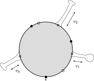
Figure 21. A single disc with forgotten points (marked with hollow circles) and homotopy units (marked with stars and dotted connect sums). The connect sums should be thought of simply as a schematic picture; really the conformal structure on the disc stays the same.

Definition 10.20.

A universal and conformally consistent choice of Floer data for glued pairs of discs with homotopy units is a choice $\mathbf{D}_{(P,\vec{v},\vec{w})}$, for every boundary identification $\mathfrak{S}$ and compatible sequential point identification $\mathfrak{T}$, and every representative $(P,\vec{v},\vec{w})$, ${}_{\mathfrak{S},\mathfrak{T}}\overline{\mathfrak{H}}_{k,l}^{F_{1},F_{2},H_{1},H_{2}}$, varying smoothly over this space, whose restriction to a boundary stratum is conformally equivalent to a Floer datum coming from lower dimensional moduli spaces. Moreover, Floer data agree to infinite order at the boundary stratum with the Floer datum obtained by gluing. Finally, we require that

• (forgotten points are forgettable) In the h($\epsilon$)-stable range, the choice of Floer datum only depends on the reduced surface $\mathcal{F}_{max}(P,\vec{v},\vec{w})$. In the h($\epsilon$)-semistable range, the Floer datum agrees with the translation-invariant Floer datum on the strip.

• (0 endpoint is forgetting) In the h($\epsilon$)-stable range, if $v_{i}=0$ or $w_{j}=0$, then after forgetting the copy of ${\mathbb{H}}$ corresponding to $p_{n_{i}}$ or $p_{m_{j}}$ respectively, the Floer datum should be isomorphic to the Floer datum on $\pi_{L,p_{n_{i}}}^{0}(S,\vec{v},\vec{w})$ or $\pi_{R,p_{m_{j}}}^{0}(S,\vec{v},\vec{w})$ respectively. In the h($\epsilon$)-semistable case, the Floer datum should be isomorphic to the translation invariant Floer datum on the respective surface.

• (1 endpoint is gluing in a unit) if $v_{i}=1$ or $w_{j}=1$, then ${\mathbb{H}}_{p_{n_{i}}}$ or ${\mathbb{H}}_{p_{m_{j}}}$ should have the standard unit datum Floer data, and the Floer datum on the main component should be isomorphic to a Floer datum on $\pi_{L,p_{n_{i}}}^{1}(P,\vec{v},\vec{w})$ or $\pi_{R,p_{m_{j}}}^{1}(P,\vec{v},\vec{w})$ respectively.

Proposition 10.8.

There exists a universal and conformally consistent choice of Floer data for glued pairs of discs with homotopy units.

Proof.

One proceeds inductively on the number of homotopy units. Suppose that we have universally and conformally consistently chosen Floer data for $|H_{1}|+|H_{2}|\leq k$ and Floer data for glued pairs of discs with at least $r+s$ marked points, with homotopy units such that $|H_{1}|+|H_{2}|=k+1$. Using the endpoint constraints described above, we have already described constraints on our Floer data on the endpoints, and codimension-1 boundary strata, so we pick some Floer datum extending these cases. Recall that this is possible because all of the spaces of choices are contractible. ∎

Remark 10.7.

Notice that the notion of h($\epsilon$)-stability depends in some cases on the chosen point in the moduli space. For example, an element $(S,\vec{v})$ of $\mathfrak{H}^{d,\{1,\ldots,d\},\emptyset}$ is only h($\epsilon$)-stable if at least two of the components of $\vec{v}$ are greater than $\epsilon$. It will not be possible to consistently inherit Floer data at zero-endpoints from the forgetful map when all (or all but one) $\vec{v}$ equal to zero. Thus we are forced to turn off stability in a neighborhood of this case.

Definition 10.21.

Let $(P,\vec{v},\vec{w})$ be a pair of glued discs with $H_{1},H_{2}$ homotopy units, and suppose we have fixed a Floer datum $\mathbf{D}$ for $(P,\vec{v},\vec{w})$. Then the associated homotopy-unit surface, denoted

(10.71) $$\mathfrak{h}(P),$$

is the iterated damped connect sum

(10.72) $$\mathfrak{h}(P):=\pi_{\mathfrak{S}}(\mathfrak{F}_{max}(P))\sharp^{v_{1}}_{p_{n_{1}}}{\mathbb{H}}_{p_{n_{1}}}\cdots\sharp^{v_{|H_{1}|}}_{p_{n_{|H_{1}|}}}{\mathbb{H}}_{p_{n_{|H_{1}|}}}\sharp^{w_{1}}_{p_{m_{1}}}{\mathbb{H}}_{p_{m_{1}}}\cdots\sharp^{w_{|H_{2}}}_{p_{m_{|H_{2}|}}}{\mathbb{H}}_{p_{m_{|H_{2}|}}}.$$

This is a (potentially nodal) surface with associated Floer data.

Definition 10.22.

An admissible Lagrangian labeling for pairs of glued discs with homotopy units and forgotten point is a labeling in the usual sense, satisfying the conditions that labellings before and after H points and F points must coincide.

The admissibility condition implies that there is an induced labeling on the associated homotopy-unit surface.

Now, suppose we have fixed a universal and consistent choice of Floer data for homotopy units. Consider a compact submanifold with corners of dimension $d$

(10.73) $$\overline{\mathcal{E}}^{d}\lhook\joinrel\relbar\joinrel\rightarrow{{}_{\mathfrak{S},\mathfrak{T}}}\overline{\mathcal{H}}_{k,l}^{F_{1},F_{2},H_{1},H_{2}}.$$

with an admissible Lagrangian labeling $\vec{L}$. In the usual fashion, fix input and output chords $\vec{x}_{in},\vec{x}_{out}$ and orbits $\vec{y}_{in}$, $\vec{y}_{out}$ for the induced marked points of the associated homotopy-unit surface $\mathfrak{h}(P,\vec{v},\vec{w})$. Define

(10.74) $$\overline{\mathcal{E}}^{d}(\vec{x}_{out},\vec{y}_{out};\vec{x}_{in},\vec{y}_{in})$$

to be the space of maps

(10.75) $$\{u:\mathfrak{h}(P,\vec{v},\vec{w}))\longrightarrow M:S\in\overline{\mathcal{E}}^{d}\}$$

satisfying Floer’s equation with respect to the Floer datum and asymptotic and boundary conditions specified by the Lagrangian labeling $\vec{L}$ and asymptotic conditions $(\vec{x}_{out},\vec{y}_{out},\vec{x}_{in},\vec{y}_{in})$.

As before, $h(\mathfrak{S},k,l)$ denote the number of boundary components of any resulting surface $\mathfrak{h}(P)$.

Lemma 10.2.

The moduli spaces $\overline{\mathcal{E}}^{d}(\vec{x}_{out},\vec{y}_{out};\vec{x}_{in},\vec{y}_{in})$ are compact, and empty for all but finitely many $(\vec{x}_{out},\vec{y}_{out})$ given fixed inputs $(\vec{x}_{in},\vec{y}_{in})$. For generically chosen Floer data, they form smooth manifolds of dimension

(10.76) $$\begin{split}\dim\overline{\mathcal{E}}^{d}(\vec{x}_{out},\vec{y}_{out};\vec{x}_{in},\vec{y}_{in}):=\sum_{x_{-}\in\vec{x}_{out}}\deg(x_{-})+&\sum_{y_{-}\in\vec{y}_{out}}\deg(y_{-})\\ +(2-h(\mathfrak{S},k,l)-|\vec{x}_{out}|-2|\vec{y}_{out}|)n&+d-\sum_{x_{+}\in\vec{x}_{in}}\deg(x_{+})-\sum_{y_{+}\in\vec{y}_{in}}\deg(y_{+}).\end{split}$$

Proof.

The usual transversality arguments, dimension calculation, and compactness results apply. ∎

In the usual fashion, when the dimension of the spaces $\overline{\mathcal{E}}^{d}(\vec{x}_{out},\vec{y}_{out};\vec{x}_{in},\vec{y}_{in})$ are zero, we use orientation lines to count (with signs) the number of points in such spaces, and associate operations

(10.77) $$(-1)^{\vec{t}}\mathbf{I}_{\overline{\mathcal{E}}^{d}}$$

from the tensor product of wrapped Floer complexes and symplectic cochain complexes where $\vec{x}_{in}$, $\vec{y}_{in}$ reside to the tensor product of the complexes where $\vec{x}_{out}$, $\vec{y}_{out}$ reside, where $\vec{t}$ is a chosen sign twisting datum.

An interesting source of submanifolds for operations comes from the entire moduli spaces

(10.78) $${}_{\mathfrak{S},\mathfrak{T}}\mathfrak{H}_{k,l}^{F_{1},F_{2},H_{1},H_{2}}$$

for an initial sequential point identification $\mathfrak{T}$.

10.7. New operations

Up until now, we have been somewhat imprecise when specifying correspondences between inputs and asymptotic boundary conditions on moduli spaces associated with operations. Let us fix some notation for a specific class of moduli spaces.

Let $\mathfrak{S}$ be a boundary identification, and let $\mathfrak{T}$ be an initial sequential boundary identification that is compatible with $\mathfrak{S}$; say it is

(10.79) $$\mathfrak{T}=\{(1,1),(2,2),\ldots,(r,r)\}$$

We previously defined an operation $\mathbf{G}_{\mathfrak{S},\mathfrak{T}}$ corresponding to the entire moduli space

(10.80) $${}_{\mathfrak{S},\mathfrak{T}}\overline{\mathcal{R}}_{k,l}.$$

Let us be precise about inputs. Given boundary marked points $z_{1},\ldots,z_{k}$, $z_{1}^{\prime},\ldots,z_{l}^{\prime}$ on each factor of our pair of discs, if $i\leq r$, define

(10.81) $$g_{\mathfrak{S}}(z_{i},z_{i}^{\prime})$$

to be the image of the pair of identified points under the gluing $\pi_{\mathfrak{S}}$. The possibilities are

• a pair of boundary input points ($\tilde{z}_{i},\tilde{z}^{\prime}_{i})$ if $z_{i}$, $z_{i}^{\prime}$ were not adjacent to a boundary identification;

• a single boundary input point $\tilde{z}_{i,i^{\prime}}$ if $z_{i}$, $z_{i}^{\prime}$ were adjacent to a single boundary identification; or

• a single interior input point $\tilde{y}_{i,i^{\prime}}$ if $z_{i}$, $z_{i}^{\prime}$ were adjacent to two boundary identifications.

Denote by

(10.82) $$g_{\mathfrak{S}}(z_{j}),g_{\mathfrak{S}}(z_{j}^{\prime})$$

the images of non-identified points under the gluing $\pi_{\mathfrak{S}}$. Then, the associated operation takes the form

(10.83) $$\mathbf{G}_{\mathfrak{S},\mathfrak{T}}((\bar{x}_{1},\ldots,\bar{x}_{r}),(x_{r+1},\ldots,x_{k}),(x_{r+1}^{\prime},\ldots,x_{l}^{\prime})),$$

where $\bar{x}_{i}$ is an asymptotic condition of the same basic type as $g_{\mathfrak{S}}(z_{i},z_{i}^{\prime})$, $x_{j}$ is a boundary asymptotic condition corresponding to $g_{\mathfrak{S}}(z_{j})$, and $x_{j}^{\prime}$ is a boundary asymptotic condition associated to $g_{\mathfrak{S}}(z_{j}^{\prime})$. This operation returns a sum of boundary asymptotic condition of the same type as $g_{\mathfrak{S}}(z_{out},z_{out}^{\prime})$, the gluing of the outputs.

To be even a bit more precise, let us move now to the operations of the above form arising in $\mathcal{W}^{2}$. Given a tuple of Lagrangians $\vec{X}=X_{1},\ldots,X_{d}$ in $\mathrm{ob\ }\mathcal{W}^{2}$, and morphisms

(10.84) $$x_{i}\in\hom(X_{i},X_{i+1}),$$

identified via the correspondence

(10.85) $$x_{i}\leftrightarrow\hat{x}_{i}$$

with a boundary asymptotic condition, pair of boundary asymptotic conditions, or interior asymptotic condition respectively, discussed in Proposition 8.4, $\mu^{d}(x_{d},\ldots,x_{1})$ is by definition the labeled operation

(10.86) $$\mathbf{G}_{\mathfrak{S}(\vec{X}),\mathfrak{T}}(\hat{x}_{1},\ldots,\hat{x}_{d})$$

in the sense of above, where we are implicitly composing with the reverse identification

(10.87) $$\hat{x}\leftrightarrow x$$

to obtain the correct output, and using the usual sequential sign twisting datum $\vec{t}_{d}=(1,\ldots,d)$. This is sensible because the boundary asymptotic type of the input $\hat{x}_{i}$ is compatible with the type of the glued marked point $g_{\mathfrak{S}(\vec{X})}(z_{i},z_{i}^{\prime})$ by construction.

With this notation in place, let us now incorporate homotopy units and forgotten points. Define the $A_{\infty}$ category

(10.88) $$\tilde{\mathcal{W}}^{2}$$

to the have the same objects as $\mathcal{W}^{2}$. Its morphisms will be identical to $\mathcal{W}^{2}$ as graded vector spaces, except for each $L$, it also contains the following formal generators:

(10.89) $$f_{L}\otimes x,\ e^{+}_{L}\otimes x\in\hom_{\tilde{\mathcal{W}}^{2}}(L\times L_{j},L\times L_{k})\mathrm{\ for\ all\ }x\in CW^{*}(L_{k},L_{j})$$

(10.90) $$x\otimes f_{L},\ x\otimes e^{+}_{L}\in\hom_{\tilde{\mathcal{W}}^{2}}(L_{j}\times L,L_{k}\times L)\mathrm{\ for\ all\ }x\in CW^{*}(L_{j},L_{k}).$$

The degrees of these generators are

(10.91) $$\deg(f_{L}\otimes x)=\deg(x\otimes f_{L}) =\deg(x)-1.$$

(10.92) $$\deg(e_{L}^{+}\otimes x)=\deg(x\otimes e_{L}^{+}) =\deg(x),$$

i.e. $f_{L}$ and $e_{L}^{+}$ should be thought of as having degrees -1 and 0 respectively. Denote the generators of the morphism space between $X$ and $X^{\prime}$ in $\tilde{\mathcal{W}}^{2}$ by $\tilde{\chi}(X,X^{\prime})$. The operations on $\tilde{\mathcal{W}}^{2}$ are as follows: Fix a label-set $\vec{X}=X_{0},\ldots,X_{d}$. As in Section 8.2, there is an associated boundary identification

(10.93) $$\mathfrak{S}(\vec{X})=\{(i,i)|X_{i}=\Delta.\}$$

Now, let $x_{1},\ldots,x_{d}$ be a sequence of asymptotic boundary conditions, i.e. $x_{i}\in\tilde{\chi}(X_{i-1},X_{i})$. Let

(10.94) $$F_{1},F_{2},H_{1},H_{2}\subset\{1,\ldots,d\}$$

denote the subset of these of the form $e^{+}_{L}\otimes x$,

(10.95) $$\begin{split}(F_{1}\cup H_{1})\cap(F_{2}\cup H_{2})&=\emptyset\\ F_{i}\cup H_{i}&=\emptyset.\end{split}$$

Then, define

(10.96) $$\mu^{d}(x_{d},\ldots,x_{1})$$

to be the operation controlled by the moduli space

(10.97) $${}_{\mathfrak{S}(\vec{X}),\mathfrak{T}}\overline{\mathfrak{H}}_{d,d}^{F_{1},F_{2},H_{1},H_{2}},$$

with labeling induced by the labeling of $\vec{X}$ as in Section 8.2 as follows: If the $k$th Lagrangian $X_{k}$ was labeled $L_{i}\times L_{j}$, then in the gluing $\pi_{\mathfrak{S}}(P)$, the left image of $\partial^{k}S$ will be labeled $L_{i}$ and the right image $\bar{\partial}^{k}S$ will be labeled $L_{j}$. If $\partial_{k}S$ was labeled $\Delta$, then it disappears under gluing so there is nothing to label. This induces a labeling for the associated homotopy-unit surface $\mathfrak{h}(P,\vec{v},\vec{w})$: since our labeling was by choice admissible, any boundary point which we forget or take damped connect sum is adjacent to boundary components with the same label.

The asymptotic conditions in the gluing

(10.98) $$\mathfrak{h}(P)$$

are as follows: in the glued surface $\pi_{\mathfrak{S}}(P)$, let $g_{\mathfrak{S}}(z_{i},z_{i}^{\prime})$ be the resulting inputs (or pair of inputs) obtained by the gluing. Then if $x_{i}$ is not a formal element, one requires these inputs to be asymptotic to the associated $\hat{x}_{i}$ as before. If $x_{i}$ is a formal element of any form, then $g_{\mathfrak{S}}(z_{i},z_{i}^{\prime})$ is a pair of boundary marked points $(\tilde{z}_{i},\tilde{z}_{i}^{\prime})$.

• if $x$ is of the form $f_{L}\otimes x$, then $\tilde{z}_{i}$ is marked as one of the $H_{1}$ points, and disappears under the damped connect sum operation. We require the other point $\tilde{z}_{i}^{\prime}$ to be asymptotic to $x$.

• if $x$ is of the form $x\otimes f_{L}$, then $\tilde{z}_{i}^{\prime}$ is marked as one of the $H_{2}$ points, and disappears under the damped connect sum operation. We require the other point $\tilde{z}_{i}^{\prime}$ to be asymptotic to $x$.

• if $x$ is of the form $e_{L}^{+}\otimes x$, then $\tilde{z}_{i}$ is marked as one of the $F_{1}$ points, and disappears under the forgetful map. We require the other point $\tilde{z}_{i}^{\prime}$ to be asymptotic to $x$.

• if $x$ is of the form $x\otimes e_{L}^{+}$, then $\tilde{z}_{i}^{\prime}$ is marked as one of the $F_{2}$ points, and disappears under the forgetful map. We require the other point $\tilde{z}_{i}$ to be asymptotic to $x$.

This gives rise to a well-defined operation

(10.99) $$\mu^{d}(x_{d},\ldots,x_{1})$$

where $x_{1},\ldots,x_{d}$ are allowed to be formal elements—implicitly again, we are taking the output of this operation, and composing under the reverse association

(10.100) $$\hat{x}\leftrightarrow x.$$

In this case, we use sign twisting datum $\vec{t}_{d}=(1,\ldots,d)$, including the degrees and presence of formal elements.

One can check that degree of the associated operation is $2-d$, under the choice of gradings of the formal elements (10.91) and (10.92), for the following reason: there are no Maslov type contributions of the form $\deg(f_{L})$, but this is compensated for by any additional factor of the interval $[0,1]$ in the source abstract moduli space.

As we have constructed it, this operation is only well defined for $(d,d,F_{1},F_{2},H_{1},H_{2})$ in the f-semistable range. Hand-declare the following operations, corresponding to the f-unstable range:

(10.101) $$\mu^{k}_{\mathcal{W}^{2}}(x_{1}\otimes e^{+}_{L},\cdots,x_{k}\otimes e^{+}_{L}) :=\mu^{k}_{\mathcal{W}^{op}}(x_{1},\ldots,x_{k})\otimes e^{+}_{L}$$

$$=(-1)^{*}\mu^{k}_{\mathcal{W}}(x_{k},\ldots,x_{1})\otimes e^{+}_{L}$$

(10.102) $$\mu^{k}_{\mathcal{W}^{2}}(e^{+}_{L}\otimes x_{k},\cdots,e^{+}_{L}\otimes x_{1}) :=e^{+}_{L}\otimes\mu^{k}_{\mathcal{W}}(x_{k},\ldots,x_{1})$$

(10.103) $$\mu^{1}_{\mathcal{W}^{2}}(x\otimes e^{+}_{L}) :=\mu^{1}_{\mathcal{W}}(x)\otimes e^{+}_{L}$$

(10.104) $$\mu^{1}(e^{+}_{L}\otimes x) :=e^{+}_{L}\otimes\mu^{1}_{\mathcal{W}}(x)$$

(10.105) $$\mu^{1}_{\mathcal{W}^{2}}(f_{L}\otimes x) :=(e^{+}_{L}-e_{L})\otimes x\pm f_{L}\otimes\mu^{1}_{\mathcal{W}}(x)$$

(10.106) $$\mu^{1}_{\mathcal{W}^{2}}(x\otimes f_{L}) :=x\otimes(e^{+}_{L}-e_{L})\pm\mu^{1}_{\mathcal{W}}(x)\otimes f_{L}.$$

Proposition 10.9.

The resulting category $\tilde{\mathcal{W}}^{2}$ is an $A_{\infty}$ category.

Proof.

We need to verify the $A_{\infty}$ equations hold on sequences of morphisms that include the formal elements $x\otimes e^{+}$, $e^{+}\otimes x$, $f\otimes x$, $x\otimes f$. This is mostly a consequence of the codimension-1 boundary of moduli spaces of homotopy-unit maps, although some cases (corresponding to bubbling of $f$-unstable components) will need to be checked by hand. Without loss of generality, we can assume that our original category contained just one Lagrangian $L$, so $\mathrm{ob\ }\mathcal{W}^{2}=\{L\times L,\Delta\}$; the multi-Lagrangians case is identical but slightly more notationally complex. The codimension 1 boundary of the abstract moduli space

(10.107) $${{}_{\mathfrak{S},\mathfrak{T}_{max}}}\overline{\mathfrak{H}}_{k,l}^{F_{1},F_{2},H_{1},H_{2}}$$

is covered by the following strata:

• 0 and 1 endpoints

  (10.108) $${{}_{\mathfrak{S},\mathfrak{T}_{max}}}\overline{\mathfrak{H}}_{d,d}^{F_{1},F_{2},H_{1},H_{2}}|_{v_{i}\in\{0,1\}},{{}_{\mathfrak{S},\mathfrak{T}_{max}}}\overline{\mathfrak{H}}_{d,d}^{F_{1},F_{2},H_{1},H_{2}}|_{w_{j}\in\{0,1\}},$$

• nodal degenerations:

  (10.109) $${{}_{\mathfrak{S}^{\prime},\mathfrak{T}_{max}}}\overline{\mathfrak{H}}_{d^{\prime},d^{\prime}}^{F_{1}^{\prime},F_{2}^{\prime},H_{1}^{\prime},H_{2}^{\prime}}\times{{}_{\mathfrak{S}^{\prime\prime},\mathfrak{T}_{max}}}\overline{\mathfrak{H}}_{d-d^{\prime}+1,d-d^{\prime}+1}^{F_{1}^{\prime\prime},F_{2}^{\prime\prime},H_{1}^{\prime\prime},H_{2}^{\prime\prime}}$$

Here, the boundary marked points in ${{}_{\mathfrak{S}^{\prime},\mathfrak{T}_{max}}}\overline{\mathfrak{H}}_{d^{\prime},d^{\prime}}^{F_{1}^{\prime},F_{2}^{\prime},H_{1}^{\prime},H_{2}^{\prime}}$ consist of some subsequence of length $d^{\prime}$ of $(z_{1},z_{1}^{\prime}),\ldots,(z_{d},z_{d}^{\prime})$ along with inherited $F$/$H$ labels, and the boundary marked points of ${{}_{\mathfrak{S}^{\prime\prime},\mathfrak{T}_{max}}}\overline{\mathfrak{H}}_{d-d^{\prime}+1,d-d^{\prime}+1}^{F_{1}^{\prime\prime},F_{2}^{\prime\prime},H_{1}^{\prime\prime},H_{2}^{\prime\prime}}$ consist of the sequence $(z_{1},z_{1}^{\prime}),\ldots,(z_{d},z_{d}^{\prime})$ where the chosen subsequence is replaced by a single new point $(z_{new},z_{new}^{\prime})$ (again with inherited $F$/$H$ labels).

This implies that the boundary of the one-dimensional space of maps will consist of compositions of operations coming from these strata as well as various strip-breaking operations, corresponding to pre and post-composing with $\mu^{1}$ in all possible ways.

By the choices we have made in our Floer datum, the 0 endpoint for a point $p_{n_{i}}\in H_{1}$ correspond to the operation of forgetting the point $p_{n_{i}}$, which changes the formal asymptotic condition from $f_{L}$ to $e_{L}^{+}$. The 1 end point corresponds to gluing in a geometric unit to an existing $A_{\infty}$ operation, i.e. the formal condition $f_{L}$ is replaced by an actual asymptotic condition $e_{L}$. In conjunction we see that the endpoint strata account for the occurrences of $\mu^{1}$ for the $f_{L}$ as formally defined above.

The nodal degenerations strata ensure that the associated operation is a genuine composition of the form $\mu^{d-d^{\prime}+1}(\cdots\mu^{d^{\prime}}(\cdots)\cdots)$ when both components of the strata are $f$-semistable. Let us without loss of generality suppose an $f$-unstable component bubbles off, consisting of a subsequence of the form $(z_{i+1},z_{i+1}^{\prime}),\ldots,(z_{i+d^{\prime}},z_{i+d^{\prime}}^{\prime})$, with all of the right factored pointed labeled as forgotten, with adjacent boundary components labeled by $L$. By construction such a sequence corresponds to inputs $x_{i+1}\otimes e^{+}_{L},\ldots,x_{i+d^{\prime}}\otimes e^{+}_{L}$. In the induced forgetful/gluing map, the right disc consists entirely of points labeled forgotten and is thus deleted by $f$-stabilization. Moreover, the right input of the lower disc $z_{new}^{\prime}$ is marked as forgotten. The left disc survives, contributing a $(\mu^{d^{\prime}}_{\mathcal{W}})^{op}$. We conclude that the operation associated to the top stratum is $(-1)^{*}\mu^{d^{\prime}}(x_{i+1^{\prime}},\ldots,x_{i+d^{\prime}})\otimes e^{+}_{L}$, which equals $\mu^{d^{\prime}}(x_{i+d^{\prime}}\otimes e^{+}_{L},\ldots,x_{i+1}\otimes e^{+}_{L})$ as desired. ∎

We call the data that we have just constructed the structure of one-sided homotopy units for the category $\mathcal{W}^{2}$.

Proposition 10.10.

The modified category $\tilde{\mathcal{W}}^{2}$ is quasi-equivalent to $\mathcal{W}^{2}$.

Proof.

By construction, the inclusion

(10.110) $$\mathcal{I}:\mathcal{W}^{2}\lhook\joinrel\relbar\joinrel\rightarrow\tilde{\mathcal{W}}^{2}$$

is the desired quasi-isomorphism. If $\mu^{1}_{\mathcal{W}}(x)=0$, the elements $e^{+}_{L}\otimes x,x\otimes e^{+}_{L}$, which are the only potentially new elements of cohomology, are homologous to $e_{L}\otimes x$, $x\otimes e_{L}$. ∎

In order to simplify notation, define the total homotopy unit

(10.111) $$e^{+}:=\sum_{L\in\mathrm{ob\ }\mathcal{W}}e^{+}_{L},$$

thought of as an element in the semi-simple ring version of $\mathcal{W}$. The corresponding elements in $\mathcal{W}^{2}$ are the total one-sided units

(10.112) $$\begin{split}e^{+}\otimes x:=\sum_{L\in\mathrm{ob\ }\mathcal{W}}e^{+}_{L}\otimes x\\ x\otimes e^{+}:=\sum_{L\in\mathrm{ob\ }\mathcal{W}}x\otimes e^{+}_{L}\end{split}$$

10.8. Shuffle identities

The technology we have introduced, and the analyses of the previous section give some morphisms involving the $e^{+}$ desirable properties. To state them, we first recall the combinatorial notion of a shuffle:

Definition 10.23.

Let $V$ be a graded vector space. The $(k,l)$ shuffle of an ordered collections of elements $\{a_{1},\ldots,a_{k}\}$ and $\{b_{1},\ldots,b_{l}\}$ is defined to be following element in the tensor algebra $TV$:

(10.113) $$\mathcal{S}_{k,l}(\{a_{i}\},\{b_{j}\}):=\sum_{\sigma\in\mathrm{shuff}(\{a_{i}\},\{b_{j}\})}(-1)^{sgn(\sigma)}\sigma(a_{1}\otimes\cdots\otimes a_{k}\otimes b_{1}\otimes\cdots b_{l}).$$

Above, $\mathrm{shuff}(\{a_{i}\},\{b_{j}\})$ is the collection of permutations of the set $\{a_{1},\ldots,a_{k},b_{1},\ldots,b_{l}\}$ that preserve the relative orderings of the $a_{i}$ and $b_{j}$, $\sigma$ is the corresponding permutation on the tensor algebra, and the sign $sgn(\sigma)$ is the sign of the graded permutation, i.e. the ordinary sign of the permutation plus a sign of parity the sums of degrees of elements that have been permuted past one another.

The following Proposition, essential for our forthcoming argument, is the main consequence of the technology of one-sided homotopy units.

Proposition 10.11.

We have the following identities in $\tilde{\mathcal{W}}^{2}$:

(10.114) $$\mu^{k+l}_{\tilde{\mathcal{W}}^{2}}(\mathcal{S}_{k,l}(\{x_{i}\otimes e^{+}\}_{i=k}^{1};\{e^{+}\otimes y_{j}\}_{j=1}^{l})) =0,\mathrm{\ for\ }k,\ l>0$$

(10.115) $$\mu^{k+l+1}_{\tilde{\mathcal{W}}^{2}}(\hat{\mathbf{a}},\mathcal{S}_{k,l}(\{x_{i}\otimes e^{+}\}_{i=k}^{1};\{e^{+}\otimes y_{j}\}_{j=1}^{l})) =\mu^{k+l+1}_{\mathcal{W}}(x_{1},\ldots,x_{k},\mathbf{a},y_{1},\ldots,y_{l})$$

(10.116) $$\mu^{k+l+1}_{\tilde{\mathcal{W}}^{2}}(\mathcal{S}_{k,l}(\{x_{i}\otimes e^{+}\}_{i=k}^{1};\{e^{+}\otimes y_{j}\}_{j=1}^{l}),\hat{\mathbf{b}}) =\mu^{k+l+1}_{\mathcal{W}}(y_{1},\ldots,y_{l},\mathbf{b},x_{1},\ldots,x_{k})$$

(10.117) $$\mu^{k+l+2}_{\tilde{\mathcal{W}}^{2}}(\hat{\mathbf{a}},\mathcal{S}_{k,l}(\{x_{i}\otimes e^{+}\}_{i=k}^{1};\{e^{+}\otimes y_{j}\}_{j=1}^{l},\hat{\mathbf{b}}) =\mathrm{}_{2}\mathcal{OC}(\mathbf{a},y_{1},\ldots,y_{l},\mathbf{b},x_{1},\ldots,x_{k})$$

where $\mathbf{b}\in\hom(\Delta,L_{i}\times L_{j})$ and $\mathbf{a}\in\hom(L_{i}\times L_{j},\Delta)$ respectively.

Proof.

This is the content of Propositions 10.3, 10.4, 10.5, and 10.6 except for the case of (10.114) when $k=l=1$. In that case, we have that

(10.118) $$\begin{split}\mu^{2}_{\tilde{\mathcal{W}}^{2}}(\mathcal{S}_{1,1}(\{x\otimes e^{+}\};\{e^{+}\otimes y\})&=\mu^{2}_{\tilde{\mathcal{W}}^{2}}(x\otimes e^{+},e^{+}\otimes y)-\mu^{2}_{\tilde{\mathcal{W}}^{2}}(e^{+}\otimes y,x\otimes e^{+})\\ &=x\otimes y-x\otimes y\\ &=0.\end{split}$$

∎

11. Split-resolving the diagonal

In this section, we prove the following theorem.

Theorem 11.1.

If $M$ is non-degenerate, the product Lagrangians $\{L_{i}\times L_{j}\}$ split-generate $\Delta$ in the category $\mathcal{W}^{2}$.

The proof uses a criterion for split generation discussed in Section 2.12, which we now recall. Let $\mathcal{W}^{2}_{split}$ be the full sub-category of $\mathcal{W}^{2}$ with objects given by the product Lagrangians $\{L_{i}\times L_{j}\}$. There is a natural bar complex

(11.1) $$\mathcal{Y}^{r}_{\Delta}\otimes_{\mathcal{W}^{2}_{split}}\mathcal{Y}^{l}_{\Delta}$$

and collapse map

(11.2) $$\mu:\mathcal{Y}^{r}_{\Delta}\otimes_{\mathcal{W}^{2}_{split}}\mathcal{Y}^{l}_{\Delta}\longrightarrow\hom_{\mathcal{W}^{2}}(\Delta,\Delta).$$

If $H^{*}(\mu)$ hits the unit element $[e]\in\hom_{\mathcal{W}^{2}}(\Delta,\Delta)=SH^{*}(M)$, then we can conclude that the product Lagrangians split-generate $\Delta$.

Because split-generation is invariant under quasi-isomorphisms, it will suffice to establish the above claim in the category

(11.3) $$\tilde{\mathcal{W}}^{2}$$

which is quasi-isomorphic to $\mathcal{W}$.

Define a map

(11.4) $$\Gamma:\ _{2}\mathrm{CC}_{*}(\mathcal{W},\mathcal{W})\longrightarrow\mathcal{Y}^{r}_{\Delta}\otimes_{\tilde{W}^{2}_{split}}\mathcal{Y}^{l}_{\Delta}$$

as follows:

(11.5) $$\begin{split}\Gamma:\mathbf{a}\otimes b_{1}\otimes\ldots\otimes&b_{l}\otimes\mathbf{b}\otimes a_{1}\otimes\cdots\otimes a_{k}\longmapsto\\ &(-1)^{\blacksquare}\hat{\mathbf{a}}\otimes\mathcal{S}_{k,l}((a_{k}\otimes e^{+},\ldots,a_{1}\otimes e^{+});(e^{+}\otimes b_{1},\ldots,e^{+}\otimes b_{l}))\otimes\hat{\mathbf{b}}.\end{split}$$

where $\mathcal{S}_{k,l}$ is the $(k,l)$ shuffle product defined in the previous section, and $\hat{\mathbf{a}}$ refers to $\mathbf{a}$ thought of as an element of $\hom(L_{i}\times L_{j},\Delta)$ instead of $\hom(L_{j},L_{i})$, and similarly for $\hat{\mathbf{b}}$ under the usual correspondence from Proposition 8.4. The Koszul sign

(11.6) $$\blacksquare:=\sum_{j=k}^{1}\bigg{(}||a_{j}||\cdot\big{(}\sum_{i=j-1}^{1}||a_{i}||+|\mathbf{b}|\big{)}\bigg{)}$$

can be thought of as arising from rearranging the substrings of the Hochschild chain $\mathbf{a},b_{1},\ldots,b_{l}$ and $\mathbf{b},a_{1},\ldots,a_{k}$ so that they are superimposed, with the latter sequence in reverse order.

Proposition 11.1.

$\Gamma$ is a chain map.

Proof.

We verify this proposition up to sign. Using Proposition 10.11, we must show that $\Gamma$ intertwines the two-pointed Hochschild differential with the bar complex differential on $\tilde{\mathcal{W}}^{2}$. Abbreviate the shuffle product

(11.7) $$\mathcal{S}_{i,j}(\{a_{s}\otimes e^{+}\}_{s=r+i}^{r+1};\{e^{+}\otimes b_{t}\}_{t=n+1}^{n+j})$$

by

(11.8) $$\mathcal{S}(a_{r+i\rightarrow r+1};b_{n+1\rightarrow n+j})$$

The bar differential applied to

(11.9) $$\Gamma(\mathbf{a}\otimes b_{1}\otimes\cdots\otimes b_{l}\otimes\mathbf{b}\otimes a_{1}\otimes\cdots\otimes a_{k})$$

is the sum of the following terms (with Koszul signs described in (2.222) that are omitted):

(11.10) $$\sum_{i\geq 0,j\geq 0}\mu_{\tilde{\mathcal{W}}^{2}}(\hat{\mathbf{a}},\mathcal{S}(a_{k\rightarrow k-i+1};b_{1\rightarrow j}))\otimes\mathcal{S}(a_{k-i\rightarrow 1};b_{j\rightarrow l})\otimes\hat{\mathbf{b}}\ \ \ \textrm{(collapse on left)}$$

(11.11) $$\sum_{i\geq 0,j\geq 0}\hat{\mathbf{a}}\otimes\mathcal{S}(a_{k\rightarrow k-i+1};b_{1\rightarrow j})\otimes\mu_{\tilde{\mathcal{W}}^{2}}(\mathcal{S}(a_{k-i\rightarrow 1};b_{j+1\rightarrow l}),\hat{\mathbf{b}})\ \ \ \textrm{(collapse on right)}$$

(11.12) $$\sum_{i_{0},i_{1},j_{0},j_{1}}\hat{\mathbf{a}}\otimes\mathcal{S}(a_{k\rightarrow k-i_{0}+1};b_{1\rightarrow j_{0}})\otimes\mu_{\tilde{\mathcal{W}}^{2}}(\mathcal{S}(a_{k-i_{0}\rightarrow k-i_{0}-i_{1}+1};b_{j_{0}+1\rightarrow j_{0}+j_{1}}))$$

$$\ \ \ \ \ \ \ \ \ \ \ \ \ \otimes\mathcal{S}(a_{k-i_{0}-i_{1}\rightarrow 1};b_{j_{0}+j_{1}+1\rightarrow l})\otimes\hat{\mathbf{b}}\ \ \ \textrm{(collapse in middle)}.$$

By Proposition 10.11,

(11.13) $$\mu_{\tilde{\mathcal{W}}^{2}}(\hat{\mathbf{a}},\mathcal{S}(a_{k\rightarrow k-i+1};b_{1\rightarrow j})) =\mu^{i+j+1}_{\mathcal{W}}(a_{k-i+1},\ldots,a_{k},\mathbf{a},b_{1},\ldots,b_{j})$$

(11.14) $$\mu_{\tilde{\mathcal{W}}^{2}}(\mathcal{S}(a_{k-i\rightarrow 1};b_{j+1\rightarrow l}),\hat{\mathbf{b}}) =\mu^{(k-i)+(l-j)+1}_{\mathcal{W}}(b_{j+1},\ldots,b_{l},\mathbf{b},a_{1},\ldots,a_{k-i})$$

and

(11.15) $$\begin{split}\mu_{\tilde{\mathcal{W}}^{2}}(\mathcal{S}(a_{k-i_{0}\rightarrow k-i_{0}-i_{1}+1};&b_{j_{0}+1\rightarrow j_{0}+j_{1}}))=\\ &\begin{cases}0&i_{1}\geq 1\textrm{ and }j_{1}\geq 1\\ \mu^{i_{1}}_{\mathcal{W}}(a_{k-i_{0}-i_{1}},\ldots,a_{k-i_{0}})\otimes e^{+}&j_{1}=0\\ e^{+}\otimes\mu^{j_{1}}(b_{j_{0}+1},\ldots,b_{j_{0}+j_{1}})&i_{1}=0\end{cases}\end{split}$$

Putting this all together, we see that the non-zero terms above comprise exactly the terms in

(11.16) $$\Gamma\circ d_{{{}_{2}}\mathrm{CC}}(\mathbf{a}\otimes a_{1}\otimes\cdots\otimes a_{k}\otimes\mathbf{b}\otimes b_{1}\otimes\cdots\otimes b_{l}).$$

∎

The following Proposition completes the proof of Theorem 11.1.

Proposition 11.2.

There is a commutative diagram of chain complexes

(11.17)

where $D$ is the identity map (by our definition of $\hom(\Delta,\Delta)$).

Proof.

This is also a corollary of Proposition 10.11. Namely, we showed there that

(11.18) $$\begin{split}\mu(\hat{\mathbf{a}},\mathcal{S}_{k,l}(a_{k}\otimes e^{+},\ldots,a_{1}\otimes e^{+});(e^{+}\otimes b_{1},&\ldots,e^{+}\otimes b_{l}),\hat{\mathbf{b}})=\\ &{{}_{2}}\mathcal{OC}(\hat{\mathbf{a}},b_{1},\ldots,b_{l},\hat{\mathbf{b}},a_{1},\ldots,a_{k}),\end{split}$$

a restatement of (11.17). ∎

Proof of Theorem 11.1.

If the map $[\mathcal{CO}]:\mathrm{HH}_{*}(\mathcal{W},\mathcal{W})\longrightarrow SH^{*}(M)$ hits $[e]$, we conclude first that the representing chain-map ${{}_{2}}\mathcal{CO}:{{}_{2}}\mathrm{CC}_{*}(\mathcal{W},\mathcal{W})\longrightarrow CH^{*}(M)$ hits a representative $[e]$. Thus by the existence of the diagram (11.17), $H^{*}(\mu)$ hits $[e]\in HW^{*}(\Delta,\Delta)$, verifying the split-generation criterion (2.226) for $\Delta$. ∎

Corollary 11.1 ($\mathbf{M}$ is full on $\mathcal{W}^{2}$).

Assuming non-degeneracy, $\mathbf{M}$ is full on $\mathcal{W}^{2}$.

Proof.

We have shown that if $M$ is non-degenerate, then $\Delta$ is split-generated by the product Lagrangians $\{L_{i}\times L_{j}\}$. We have also constructed an $A_{\infty}$ functor,

(11.19) $$\mathbf{M}:\mathcal{W}^{2}\longrightarrow\mathcal{W}\mathrm{\!-\!mod\!-\!}\mathcal{W}$$

and we have shown that $\mathbf{M}$ takes product Lagrangians $\{L_{i}\times L_{j}\}$ to Yoneda bimodules $\mathcal{Y}^{l}_{L_{i}}\otimes\mathcal{Y}^{r}_{L_{j}}$, and is full on these objects. This is the content of Propositions 9.3, 9.4, and 9.5. Thus, by Proposition 2.8, we conclude $\mathbf{M}$ is full on $\{\Delta,\{L_{i}\times L_{j}\}\}$. ∎

Proof of Theorem 1.2.

We showed in Proposition 9.6 that $\mathbf{M}$ sends $\Delta$ to the diagonal bimodule $\mathcal{W}_{\Delta}$. Thus, by Corollary 11.1, we conclude that $\mathcal{W}_{\Delta}$ is split-generated by Yoneda bimodules, the definition of homological smoothness. ∎

Corollary 11.2.

The maps

(11.20) $$\begin{split}\mathcal{CO}:SH^{*}(M)&\longrightarrow\mathrm{HH}^{*}(\mathcal{W},\mathcal{W})\\ {}_{2}\mathcal{CO}:SH^{*}(M)&\longrightarrow{{}_{2}}\mathrm{HH}^{*}(\mathcal{W},\mathcal{W})\\ \end{split}$$

are isomorphisms.

Proof.

By Proposition 9.7, the map ${}_{2}\mathcal{CO}$ is exactly the first order map

(11.21) $$\mathbf{M}^{1}:HW^{*}(\Delta,\Delta)\longrightarrow\hom_{\mathcal{W}\!-\!\mathcal{W}}(\mathcal{W}_{\Delta},\mathcal{W}_{\Delta}),$$

and $\mathbf{M}$ is full on $\Delta$. ∎

Remark 11.1.

In fact, there is also a commutative diagram of the form

(11.22) $$\lx@xy@svg{\hbox{\raise 0.0pt\hbox{\kern 64.06537pt\hbox{\ignorespaces\ignorespaces\ignorespaces\hbox{\vtop{\kern 0.0pt\offinterlineskip\halign{\entry@#!@&&\entry@@#!@\cr&\\&\crcr}}}\ignorespaces{\hbox{\kern-64.06537pt\raise 0.0pt\hbox{\hbox{\kern 0.0pt\raise 0.0pt\hbox{\hbox{\kern 3.0pt\raise 0.0pt\hbox{$\textstyle{\mathrm{CC}_{*}(\mathcal{W}^{op},\mathcal{W}^{op})\otimes_{{\mathbb{K}}}\mathrm{CC}_{*}(\mathcal{W},\mathcal{W})\ignorespaces\ignorespaces\ignorespaces\ignorespaces\ignorespaces\ignorespaces\ignorespaces\ignorespaces}$}}}}}}}\ignorespaces\ignorespaces\ignorespaces\ignorespaces{}{\hbox{\lx@xy@droprule}}\ignorespaces\ignorespaces\ignorespaces{\hbox{\kern 43.00871pt\raise 5.39166pt\hbox{{}\hbox{\kern 0.0pt\raise 0.0pt\hbox{\hbox{\kern 3.0pt\hbox{\hbox{\kern 0.0pt\raise-2.39166pt\hbox{$\scriptstyle{\ \ \ \ \ \ \ \Omega}$}}}\kern 3.0pt}}}}}}\ignorespaces{\hbox{\kern 96.31737pt\raise 0.0pt\hbox{\hbox{\kern 0.0pt\raise 0.0pt\hbox{\lx@xy@tip{1}\lx@xy@tip{-1}}}}}}{\hbox{\lx@xy@droprule}}{\hbox{\lx@xy@droprule}}\ignorespaces\ignorespaces\ignorespaces\ignorespaces{}{\hbox{\lx@xy@droprule}}\ignorespaces\ignorespaces\ignorespaces{\hbox{\kern 0.0pt\raise-20.67401pt\hbox{{}\hbox{\kern 0.0pt\raise 0.0pt\hbox{\hbox{\kern 3.0pt\hbox{\hbox{\kern 0.0pt\raise-2.1pt\hbox{$\scriptstyle{\mathcal{OC}\otimes\mathcal{OC}}$}}}\kern 3.0pt}}}}}}\ignorespaces{\hbox{\kern 0.0pt\raise-30.21194pt\hbox{\hbox{\kern 0.0pt\raise 0.0pt\hbox{\lx@xy@tip{1}\lx@xy@tip{-1}}}}}}{\hbox{\lx@xy@droprule}}{\hbox{\lx@xy@droprule}}{\hbox{\kern 96.31737pt\raise 0.0pt\hbox{\hbox{\kern 0.0pt\raise 0.0pt\hbox{\hbox{\kern 3.0pt\raise 0.0pt\hbox{$\textstyle{\mathrm{CC}_{*}(\tilde{\mathcal{W}}^{2}_{split},\tilde{\mathcal{W}}^{2}_{split})\ignorespaces\ignorespaces\ignorespaces\ignorespaces}$}}}}}}}\ignorespaces\ignorespaces\ignorespaces\ignorespaces{}{\hbox{\lx@xy@droprule}}\ignorespaces\ignorespaces\ignorespaces{\hbox{\kern 121.57297pt\raise-20.67401pt\hbox{{}\hbox{\kern 0.0pt\raise 0.0pt\hbox{\hbox{\kern 3.0pt\hbox{\hbox{\kern 0.0pt\raise-3.0361pt\hbox{$\scriptstyle{\mathcal{OC}^{2}}$}}}\kern 3.0pt}}}}}}\ignorespaces{\hbox{\kern 121.57297pt\raise-30.21194pt\hbox{\hbox{\kern 0.0pt\raise 0.0pt\hbox{\lx@xy@tip{1}\lx@xy@tip{-1}}}}}}{\hbox{\lx@xy@droprule}}{\hbox{\lx@xy@droprule}}{\hbox{\kern-49.46802pt\raise-41.34804pt\hbox{\hbox{\kern 0.0pt\raise 0.0pt\hbox{\hbox{\kern 3.0pt\raise 0.0pt\hbox{$\textstyle{CH^{*}(M^{-})\otimes_{\mathbb{K}}CH^{*}(M)\ignorespaces\ignorespaces\ignorespaces\ignorespaces}$}}}}}}}\ignorespaces\ignorespaces\ignorespaces\ignorespaces{}{\hbox{\lx@xy@droprule}}\ignorespaces\ignorespaces\ignorespaces{\hbox{\kern 49.81425pt\raise-37.06398pt\hbox{{}\hbox{\kern 0.0pt\raise 0.0pt\hbox{\hbox{\kern 3.0pt\hbox{\hbox{\kern 0.0pt\raise-1.28406pt\hbox{$\scriptstyle{\ \ \ =}$}}}\kern 3.0pt}}}}}}\ignorespaces{\hbox{\kern 88.06537pt\raise-41.34804pt\hbox{\hbox{\kern 0.0pt\raise 0.0pt\hbox{\lx@xy@tip{1}\lx@xy@tip{-1}}}}}}{\hbox{\lx@xy@droprule}}{\hbox{\lx@xy@droprule}}{\hbox{\kern 88.06537pt\raise-41.34804pt\hbox{\hbox{\kern 0.0pt\raise 0.0pt\hbox{\hbox{\kern 3.0pt\raise 0.0pt\hbox{$\textstyle{CH^{*}(M^{-}\times M)}$}}}}}}}\ignorespaces}}}}\ignorespaces, \textstyle{\mathrm{CC}_{*}(\mathcal{W}^{op},\mathcal{W}^{op})\otimes_{{\mathbb{K}}}\mathrm{CC}_{*}(\mathcal{W},\mathcal{W})\ignorespaces\ignorespaces\ignorespaces\ignorespaces\ignorespaces\ignorespaces\ignorespaces\ignorespaces} \scriptstyle{\ \ \ \ \ \ \ \Omega} \scriptstyle{\mathcal{OC}\otimes\mathcal{OC}} \textstyle{\mathrm{CC}_{*}(\tilde{\mathcal{W}}^{2}_{split},\tilde{\mathcal{W}}^{2}_{split})\ignorespaces\ignorespaces\ignorespaces\ignorespaces} \scriptstyle{\mathcal{OC}^{2}} \textstyle{CH^{*}(M^{-})\otimes_{\mathbb{K}}CH^{*}(M)\ignorespaces\ignorespaces\ignorespaces\ignorespaces} \scriptstyle{\ \ \ =} \textstyle{CH^{*}(M^{-}\times M)} \textstyle{\mathrm{CC}_{*}(\mathcal{W}^{op},\mathcal{W}^{op})\otimes_{{\mathbb{K}}}\mathrm{CC}_{*}(\mathcal{W},\mathcal{W})\ignorespaces\ignorespaces\ignorespaces\ignorespaces\ignorespaces\ignorespaces\ignorespaces\ignorespaces} \scriptstyle{\ \ \ \ \ \ \ \Omega} \scriptstyle{\mathcal{OC}\otimes\mathcal{OC}} \textstyle{\mathrm{CC}_{*}(\tilde{\mathcal{W}}^{2}_{split},\tilde{\mathcal{W}}^{2}_{split})\ignorespaces\ignorespaces\ignorespaces\ignorespaces} \scriptstyle{\mathcal{OC}^{2}} \textstyle{CH^{*}(M^{-})\otimes_{\mathbb{K}}CH^{*}(M)\ignorespaces\ignorespaces\ignorespaces\ignorespaces} \scriptstyle{\ \ \ =} \textstyle{CH^{*}(M^{-}\times M)}$$

where $\mathcal{OC}^{2}$ is the open-closed map on the product. The map $\Omega$ is given by sending a pair of Hochschild chains, the first in reverse order, to the shuffle of the chains:

(11.23) $$(a_{0}\otimes\cdots\otimes a_{k})\otimes(b_{l}\otimes\cdots\otimes b_{0})\longmapsto\mathcal{S}_{k+1,l+1}(a_{k}\otimes e^{+},\ldots,a_{0}\otimes e^{+};e^{+}\otimes b_{l},\ldots,e^{+}\otimes b_{0}).$$

This diagram exists on $M\times M$ with the symplectic form $(\omega,\omega)$ as well—one simply stops reversing the order of the left sequence. The conjectural implication is that if $M$ is non-degenerate, then any product $M^{k}\times(M^{-})^{l}$ is also non-degenerate, with essential Lagrangians given by products of the essential Lagrangians in $M$. The reason we have not adopted such a more general approach is that our current construction of $\mathcal{W}^{2}$ is somewhat ad hoc, only allowing the use of split Hamiltonians. As a result, most Lagrangians we might like to consider are inadmissible. Modulo this technical detail, which has already been resolved for symplectic cohomology [Oancea:2006oq], our argument applies.

Remark 11.2.

The map $\Omega$ and $\Gamma$ that we have described are generalizations of a natural product structure on the Hochschild homology of associative algebras [Loday:1992fk]*§4.2. In the setting of unital associative algebras, a version of the Eilenberg-Zilberg theorem says that shuffle product induces an isomorphism

(11.24) $$sh_{*}:\mathrm{HH}_{*}(A)\otimes\mathrm{HH}_{*}(A^{\prime})\longrightarrow\mathrm{HH}_{*}(A\otimes A^{\prime}).$$

We have described an $A_{\infty}$ version of the above morphism, which requires the strictification of units to carry through. There is a well defined quasi-inverse that always exists in the associative unital setting, and we conjecture that such quasi-inverses exist in the $A_{\infty}$ setting as well. Constructing them may involve deforming the diagonal associahedron $\Delta_{d}\subset\mathcal{R}^{d}\times\mathcal{R}^{d}$ onto various copies of products of strata in order to obtain formulas for the tensor product of $A_{\infty}$ algebras—see e.g., [Saneblidze:2004fk].

12. The non-compact Calabi-Yau structure

Assuming $\mathbf{M}$ is non-degenerate, we have shown that $\mathcal{W}$ is homologically smooth. Thus from the results in Section 2.13, the inverse dualizing bimodule,

(12.1) $$\mathcal{W}^{!}:=\hom_{\mathcal{W}\!-\!\mathcal{W}}(\mathcal{W}_{\Delta},\mathcal{W}_{\Delta}\otimes_{\mathbb{K}}\mathcal{W}_{\Delta})$$

is a perfect bimodule that represents Hochschild cohomology

(12.2) $$\mathcal{W}^{!}\otimes_{\mathcal{W}\!-\!\mathcal{W}}\mathcal{B}\simeq\mathrm{HH}^{*}(\mathcal{W},\mathcal{B}).$$

In this section, we describe a geometric morphism of bimodules.

(12.3) $$\mathcal{CY}:\mathcal{W}_{\Delta}\longrightarrow\mathcal{W}^{!}[n].$$

The construction involves operations arising from discs with two negative punctures and arbitrary numbers of positive punctures. We require that there be a distinguished positive puncture on each component of the boundary of the disc minus negative punctures; namely, we require there to be at least two inputs. Then, we interpret one of the distinguished positive punctures as belonging to $\mathcal{W}$ and the remaining distinguished input and two outputs as belonging to $\mathcal{W}^{!}$.

Definition 12.1.

The moduli space of discs with two negative punctures, two positive punctures, and $(k,l;s,t)$ positive marked points

(12.4) $$\mathcal{R}_{2}^{k,l;s,t}$$

is the abstract moduli space of discs with

• two distinguished negative marked points $z_{-}^{1}$, $z_{-}^{2}$,

• two distinguished positive marked points $z_{+}^{1}$, $z_{+}^{2}$, one removed from each boundary component cut out by $z_{-}^{1}$ and $z_{-}^{2}$,

• $k$ positive marked points $a_{1},\ldots,a_{k}$ between $z_{-}^{1}$ and $z_{+}^{1}$

• $l$ positive marked points $b_{1},\ldots,b_{l}$ between $z_{+}^{1}$ and $z_{-}^{2}$

• $s$ positive marked points $c_{1},\ldots,c_{s}$ between $z_{-}^{2}$ and $z_{+}^{2}$; and

• $t$ positive marked points $d_{1},\ldots,d_{t}$ between $z_{+}^{2}$ and $z_{-}^{1}$.

Moreover, the distinguished points $z_{-}^{1}$, $z_{-}^{2}$, $z_{+}^{1}$, and $z_{+}^{2}$ are constrained to lie (after automorphism) at $1$, $-1$, $i$ and $-i$ respectively. Namely, we fix the cross-ratios of these 4 points.

The boundary strata of the Deligne-Mumford compactification

(12.5) $$\overline{\mathcal{R}}_{2}^{k,l;s,t}$$

is covered by the images of natural inclusions of the following products:

(12.6) $$\overline{\mathcal{R}}^{k^{\prime}+1+l^{\prime}} \times_{1+}\overline{\mathcal{R}}_{2}^{k-k^{\prime},l-l^{\prime};s,t}$$

(12.7) $$\overline{\mathcal{R}}^{k^{\prime}} \times^{a}_{n+1}\overline{\mathcal{R}}_{2}^{k-k^{\prime}+1,l;s,t},\ \ \ 0\leq n<k-k^{\prime}+1$$

(12.8) $$\overline{\mathcal{R}}^{l^{\prime}} \times^{b}_{n+1}\overline{\mathcal{R}}_{2}^{k,l-l^{\prime}+1;s,t},\ \ \ 0\leq n<l-l^{\prime}+1$$

(12.9) $$\overline{\mathcal{R}}^{s^{\prime}+1+t^{\prime}} \times_{2+}\overline{\mathcal{R}}_{2}^{k,l,s-s^{\prime},t-t^{\prime}}$$

(12.10) $$\overline{\mathcal{R}}^{s^{\prime}} \times^{c}_{n+1}\overline{\mathcal{R}}_{2}^{k,l;s-s^{\prime}+1,t},\ \ \ 0\leq n<s-s^{\prime}+1$$

(12.11) $$\overline{\mathcal{R}}^{t^{\prime}} \times^{d}_{n+1}\overline{\mathcal{R}}_{2}^{k,l;s,t-t^{\prime}+1},\ \ \ 0\leq n<t-t^{\prime}+1$$

(12.12) $$\overline{\mathcal{R}}_{2}^{k-k^{\prime},l;s^{\prime},t-t^{\prime}} \times_{(1,k^{\prime}+1)}\overline{\mathcal{R}}^{k^{\prime}+1+t^{\prime}}$$

(12.13) $$\overline{\mathcal{R}}_{2}^{k,l-l^{\prime};s-s^{\prime},t} \times_{(2,s^{\prime}+1)}\overline{\mathcal{R}}^{l^{\prime}+1+s^{\prime}}.$$

Above, the notation $\times_{j+}$ in (12.6) and (12.9) indicates that the output of the first component is glued to the special input $z_{j}^{+}$ of the second component, $\times^{a}_{j}$, $\times^{b}_{j}$, $\times^{c}_{j}$ and $\times^{d}_{j}$ indicate gluing to the input $a_{j}$, $b_{j}$, $c_{j}$, and $d_{j}$ respectively, and $\times_{(i,j)}$ in (12.12) and (12.13) indicate gluing the $i$th output of the first component to the $j$th input of the second. Also, in (12.6) and (12.9), the $k^{\prime}+1$st and $s^{\prime}+1$st input points of the first component become the special points $z^{1}_{+}$ and $z^{2}_{+}$ after gluing respectively.

Figure 22. A schematic of the moduli space $\mathcal{R}^{2,3;3,2}_{2}$. All non-signed marked points are inputs.

Definition 12.2.

A Floer datum for a disc $S$ with two positive, two negative, and $(k,l;s,t)$ positive boundary marked points is a Floer datum of $S$ thought of as an open-closed string.

Fix a sequence of Lagrangians

(12.14) $$A_{0},\ldots,A_{k},B_{0},\ldots,B_{l},C_{0},\ldots,C_{s},D_{0},\ldots,D_{t},$$

corresponding to a labeling of the boundary of an element of $\mathcal{R}_{2}^{k,l;s,t}$ by specifying that $a_{i}$ be the intersection point between $A_{i-1}$ and $A_{i}$, and so on for $b_{i}$, $c_{i}$, and $d_{i}$. In the manner described in (4.27), the space $\overline{\mathcal{R}}_{2}^{k,l;s,t}$, along with the sign twisting datum

(12.15) $$\vec{t}_{\mathcal{CY}_{k,l,s,t}}:=(1,2,\ldots,k,k,k+1,\ldots,k+l,1,2,\ldots,s,s,s+1,\ldots,s+t)$$

corresponding to inputs $(a_{1},\ldots,a_{k},z_{1}^{+},b_{1},\ldots,b_{l},c_{1},\ldots,c_{s},z_{2}^{+},d_{1},\ldots,d_{t})$, determines an operation

(12.16) $$\begin{split}\mathbf{CY}_{l,k,t,s}:\big{(}\hom(B_{l-1},B_{l})&\otimes\cdots\otimes\hom(B_{0},B_{1})\\ &\otimes\mathbf{hom}(A_{k},B_{0})\otimes\hom(A_{k-1},A_{k})\otimes\cdots\otimes\hom(A_{0},A_{1})\big{)}\\ \otimes\big{(}\hom(D_{t-1},D_{t})&\otimes\cdots\otimes\hom(D_{0},D_{1})\\ &\otimes\mathbf{hom}(C_{s},D_{0})\otimes\hom(C_{s-1},C_{s})\otimes\cdots\otimes\hom(C_{0},C_{1})\big{)}\\ &\longrightarrow\mathbf{hom}(A_{0},D_{t})\otimes\mathbf{hom}(C_{0},B_{l}).\end{split}$$

Definition 12.3.

The Calabi-Yau morphism

(12.17) $$\mathcal{CY}:\mathcal{W}_{\Delta}\longrightarrow\mathcal{W}^{!}[n]$$

is given by the following data:

• For objects $(X,Y)$, a map

  (12.18) $$\begin{split}\mathcal{CY}^{0|1|0}:\mathcal{W}_{\Delta}(X,Y)&\longrightarrow\hom_{\mathcal{W}\mathrm{\!-\!mod\!-\!}\mathcal{W}}(\mathcal{W}_{\Delta},\mathcal{Y}^{l}_{X}\otimes\mathcal{Y}^{r}_{Y})\\ \mathbf{a}&\longmapsto\phi_{\mathbf{a}}\end{split}$$

  where $\phi_{\mathbf{a}}$ is the morphism whose $t|1|s$ term is

  (12.19) $$\begin{split}\phi_{\mathbf{a}}^{t|1|s}(&d_{t},\ldots,d_{1},\mathbf{b},c_{s},\ldots,c_{1}):=\\ &\mathcal{CY}_{0,0,t,s}(\mathbf{a},d_{t},\ldots,d_{1},\mathbf{b},c_{s},\ldots,c_{1})\end{split}$$

• Higher morphisms

  (12.20) $$\begin{split}\mathcal{CY}^{l|1|k}:\hom_{\mathcal{W}}(Y_{k-1},Y_{k})\otimes\cdots\otimes&\hom_{\mathcal{W}}(Y_{0},Y_{1})\otimes\mathcal{W}_{\Delta}(X_{0},Y_{0})\\ \otimes\hom_{\mathcal{W}}(X_{1},X_{0})\otimes\cdots\otimes\hom_{\mathcal{W}}(X_{l},X_{l-1})&\longrightarrow\hom_{\mathcal{W}\mathrm{\!-\!mod\!-\!}\mathcal{W}}(\mathcal{W}_{\Delta},\mathcal{Y}^{l}_{X_{k}}\otimes\mathcal{Y}^{r}_{Y_{l}})\\ (b_{l},\ldots,b_{1},\mathbf{a},a_{k},\ldots,a_{1})&\longmapsto\psi_{b_{l},\ldots,b_{1},\mathbf{a},a_{k},\ldots,a_{1}}\end{split}$$

  where $\psi=\psi_{b_{l},\ldots,b_{1},\mathbf{a},a_{k},\ldots,a_{1}}$ is the morphism whose $t|1|s$ term is

  (12.21) $$\begin{split}\phi^{t|1|s}(d_{t},&\ldots,d_{1},\mathbf{b},c_{s},\ldots,c_{1}):=\\ &\mathcal{CY}_{l,k,t,s}(b_{l},\ldots,b_{1},\mathbf{a},a_{k},\ldots,a_{1};d_{t},\ldots,d_{1},\mathbf{b},c_{s},\ldots,c_{1}).\end{split}$$

Put another way, we can in a single breath say that

(12.22) $$\begin{split}(\mathcal{CY}^{l|1|k}(b_{l},\ldots,b_{1},\mathbf{a},a_{k},\ldots,&a_{1}))^{t|1|s}(d_{t},\ldots,d_{1},\mathbf{b},c_{s},\ldots,c_{1})\\ &:=\mathcal{CY}_{l,k,t,s}(b_{l},\ldots,b_{1},\mathbf{a},a_{k},\ldots,a_{1};d_{t},\ldots,d_{1},\mathbf{b},c_{s},\ldots,c_{1}).\end{split}$$

The Gromov bordification $\overline{\mathcal{R}}_{2}^{k,l;s,t}(\vec{x}_{in},\vec{x}_{out})$ has boundary covered by the images of the Gromov bordifications of spaces of maps from the nodal domains (12.6) - (12.13), along with standard strip breaking, which put together implies that:

Proposition 12.1.

$\mathcal{CY}$ is a closed morphism of $A_{\infty}$ bimodules of degree $n$.

Proof.

We will briefly indicate how to convert the strata (12.6)-(12.13) to the equation

(12.23) $$\delta\mathcal{CY}=\mathcal{CY}\circ\hat{\mu}_{\mathcal{W}_{\Delta}}-\mu_{\mathcal{W}^{!}}\circ\hat{\mathcal{CY}}=0.$$

The strata (12.6) - (12.8) correspond to $\mathcal{CY}$ composed with various $A_{\infty}$ bimodule differentials for $\mathcal{W}_{\Delta}$. The strata (12.9) - (12.11) all correspond to the internal differential $\mu^{0|1|0}_{\mathcal{W}^{!}}$, which itself involves various pieces of the $\mathcal{W}_{\Delta}$ $A_{\infty}$ bimodule differentials for the second string of inputs. Finally, the strata (12.12) - (12.13 ) for fixed $k^{\prime}$, $l^{\prime}$, and varying over all $s^{\prime}$, $t^{\prime}$ correspond to the terms of the form $\mu^{k^{\prime}|1|0}_{\mathcal{W}^{!}}\circ\mathcal{CY}$ and $\mu^{0|1|l^{\prime}}\circ\mathcal{CY}$. The ingredients to verify signs are discussed in Section B. ∎

We now observe that to first order, the operation $\mathcal{CY}$ is controlled by a moduli space identical to one appearing in our definition of quilts:

Proposition 12.2.

For any $A,B\in\mathrm{ob\ }\mathcal{W}$, there is an equality

(12.24) $$\mathcal{CY}^{0|1|0}_{A,B}=\mathbf{M}^{1}_{\Delta,A\times B}.$$

Proof.

The maps

(12.25) $$\mathcal{CY}^{0|1|0}:\hom_{\mathcal{W}}(A,B)\longrightarrow\mathcal{W}^{!}(A,B):=\hom_{\mathcal{W}\!-\!\mathcal{W}}(\mathcal{W}_{\Delta},\mathcal{Y}^{l}_{A}\otimes\mathcal{Y}^{r}_{B})[n]$$

and

(12.26) $$\mathbf{M}^{1}:\hom_{\mathcal{W}^{2}}(\Delta,A\times B):=\hom_{\mathcal{W}}(A,B)[-n]\longrightarrow\hom_{\mathcal{W}\!-\!\mathcal{W}}(\mathcal{W}_{\Delta},\mathcal{Y}^{l}_{A}\otimes\mathcal{Y}^{r}_{B})$$

have the same source and targets, so we need to verify that the spaces controlling the Floer equations are the same. The unfolding map, $\mathbf{\Psi}_{\hat{\vec{L}}}$, defined in (9.5), when applied to a quilted strip with $(r,1,s)$ marked points, with middle label sequence $(\Delta,A\times B)$, produces a surface with two output marked points, two distinguished input marked points, a distinguished input marked point between them corresponding to $\hom(A,B)$, and then $r+1+s$ input marked points (the $r+1$st of which is distinguished) around the two outputs. This is exactly the definition of the operation given by $\mathcal{CY}_{0,0;r,s}$. See also Figure 23 for a picture of this unfolding. ∎

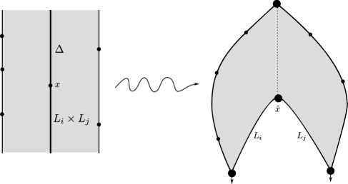
Figure 23. The equality between the quilted strip controlling $\mathbf{M}^{1}_{\Delta,L_{i}\times L_{j}}$ and the first-order map $\mathcal{CY}^{0|1|0}_{L_{i},L_{j}}$.

As an immediate corollary,

Corollary 12.1 (The wrapped Fukaya category is Calabi-Yau).

Assuming non-degeneracy, $\mathcal{CY}$ is a quasi-isomorphism.

Proof.

We have shown that under the above hypothesis $\mathbf{M}$ is full (Corollary 11.1); hence it induces isomorphisms on homology. Thus by Proposition 12.2 so does $\mathcal{CY}$. ∎

This completes the proof of Theorem 1.3.

Corollary 12.2.

For any perfect bimodule $\mathcal{B}$, there is a natural quasi-isomorphism

(12.27) $$\mathrm{HH}_{*-n}(\mathcal{W},\mathcal{B})\rightarrow\mathrm{HH}^{*}(\mathcal{W},\mathcal{B}).$$

Proof.

The isomorphism is the composition of two maps, which are both quasi-isomorphisms by Corollary 12.1 and Corollary 2.3. Using two-pointed complexes for Hochschild homology and cohomology, these maps are:

(12.28) $$\mathcal{W}_{\Delta}\otimes_{\mathcal{W}\!-\!\mathcal{W}}\mathcal{B}\stackrel{{\scriptstyle\mathcal{CY}_{\#}}}{{\longrightarrow}}\mathcal{W}^{!}\otimes_{\mathcal{W}\!-\!\mathcal{W}}\mathcal{B}\stackrel{{\scriptstyle\bar{\mu}}}{{\longrightarrow}}\hom_{\mathcal{W}\!-\!\mathcal{W}}(\mathcal{W}_{\Delta},\mathcal{B}).$$

∎

In the next section, we use Corollary 12.1 to deduce that $\mathcal{OC}:\mathrm{HH}_{*}(\mathcal{W},\mathcal{W})\rightarrow SH^{*}(M)$ is an isomorphism.

13. The Cardy condition

13.1. A geometric bimodule quasi-isomorphism

In Section 2.6, we gave a construction of a quasi-isomorphism of bimodules

(13.1) $$\mathcal{F}_{\Delta,left,right}:\mathcal{C}_{\Delta}\otimes_{\mathcal{C}}\mathcal{B}\otimes_{\mathcal{C}}\mathcal{C}_{\Delta}\stackrel{{\scriptstyle\sim}}{{\longrightarrow}}\mathcal{B}.$$

where $\mathcal{C}$ was an arbitrary $A_{\infty}$ category, $\mathcal{C}_{\Delta}$ the diagonal bimodule, and $\mathcal{B}$ a $\mathcal{C}\!-\!\mathcal{C}$ bimodule. The morphism involved collapsing on the right followed by collapsing on the left by the bimodule structure maps $\mu_{\mathcal{B}}$. The order of collapsing is of course immaterial; we have just picked one.

Let us now suppose that $\mathcal{C}=\mathcal{W}$ and $\mathcal{B}=\mathcal{W}_{\Delta}$. We would like to give a direct geometric quasi-isomorphism

(13.2) $$\mu_{LR}:\mathcal{W}_{\Delta}\otimes_{\mathcal{W}}\mathcal{W}_{\Delta}\otimes_{\mathcal{W}}\mathcal{W}_{\Delta}\longrightarrow\mathcal{W}_{\Delta},$$

homotopic to $\mathcal{F}_{\Delta,left,right}$, but not involving counts of degenerate surfaces.

Definition 13.1.

The moduli space of discs with four special points of type $(r,k,l,s)$

(13.3) $$\mathcal{R}^{r,k,l,s}$$

is the abstract moduli space of discs with $r+k+l+s+3$ positive boundary marked points and one negative boundary marked point labeled in counterclockwise order from the negative point as $(z_{out}^{-},z_{1},\ldots,z_{r},\bar{z}^{1},z_{1}^{1},\ldots,z_{k}^{1},\bar{z}^{2},z_{1}^{2},\ldots,z_{l}^{2},\bar{z}^{3},z_{1}^{3},\ldots,z_{s}^{3})$, such that

(13.4) $$\begin{split}&\textrm{after automorphism, the points }z_{out}^{-},\ \bar{z}^{1},\ \bar{z}^{2},\ \bar{z}^{3}\textrm{ lie at }\\ &-i,-1,i,\textrm{ and }1\textrm{ respectively}.\end{split}$$

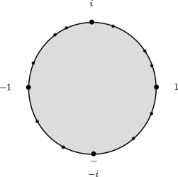
Figure 24. A schematic of the moduli space of discs with four special points of type $(2,3,3,2)$. All non-signed marked points are inputs.

The associated Floer theoretic operation to the space $\overline{\mathcal{R}}^{r,k,l,s}$ with sign twisting datum

(13.5) $$\begin{split}\vec{t}_{LR,r,k,l,s}=&(1,2,\ldots,r,r,r+1,\ldots,r+k,r+k,\\ &r+k+1,\ldots,r+k+l,r+k+l,r+k+1+1,\ldots,\\ &r+k+l+s).\end{split}$$

is

(13.6) $$\begin{split}(\mu_{LR})_{r,k,l,s}:=(-1)^{\vec{t}_{LR,r,k,l,s}}&\mathbf{F}_{\mathcal{R}^{r,k,l,s}}:\\ &\mathcal{W}^{\otimes r}\otimes\mathcal{W}_{\Delta}\otimes\mathcal{W}^{\otimes k}\otimes\mathcal{W}_{\Delta}\otimes\mathcal{W}^{\otimes l}\otimes\mathcal{W}_{\Delta}\otimes\mathcal{W}^{\otimes s}\longrightarrow\mathcal{W}_{\Delta}\end{split}$$

Then, define the morphism

(13.7) $$\mu_{LR}^{r|1|s}:=\bigoplus_{k\geq 0,l\geq 0}(\mu_{LR})_{r,k,l,s}:\mathcal{W}^{\otimes r}\otimes(\mathcal{W}_{\Delta}\otimes T\mathcal{W}\otimes\mathcal{W}_{\Delta}\otimes T\mathcal{W}\otimes\mathcal{W}_{\Delta})\otimes\mathcal{W}^{\otimes s}\longrightarrow\mathcal{W}_{\Delta}.$$

One can calculate that the morphism is degree zero, as desired.

Proposition 13.1.

The pre-morphism of bimodules

(13.8) $$\mu_{LR}\in\hom_{\mathcal{W}\!-\!\mathcal{W}}(\mathcal{W}_{\Delta}\otimes_{\mathcal{W}}\mathcal{W}_{\Delta}\otimes_{\mathcal{W}}\otimes\mathcal{W}_{\Delta},\mathcal{W}_{\Delta})$$

is closed, i.e.

(13.9) $$\delta\mu_{LR}=0.$$

Proof.

We leave this mostly as an exercise, but this follows from analyzing the equations arising from the boundary of the one-dimensional space of maps with domain $\overline{\mathcal{R}}^{r,k,l,s}$. The relevant codimension 1 boundary components involve strip-breaking and the codimension 1 boundary strata of the abstract moduli space $\overline{\mathcal{R}}^{r,k,l,s}$, which is covered by

(13.10) $$\overline{\mathcal{R}}^{r^{\prime}} \times_{n+1}\overline{\mathcal{R}}^{r-r^{\prime}+1,k,l,s},\ \ \ 0\leq n<r-r^{\prime}+1$$

(13.11) $$\overline{\mathcal{R}}^{k^{\prime}} \times^{1}_{n+1}\overline{\mathcal{R}}^{r,k-k^{\prime}+1,l,s},\ \ \ 0\leq n<k-k^{\prime}+1$$

(13.12) $$\overline{\mathcal{R}}^{l^{\prime}} \times^{2}_{n+1}\overline{\mathcal{R}}^{r,k,l-l^{\prime}+1,s},\ \ \ 0\leq n<l-l^{\prime}+1$$

(13.13) $$\overline{\mathcal{R}}^{s^{\prime}} \times^{3}_{n+1}\overline{\mathcal{R}}^{r,k,l,s-s^{\prime}+1},\ \ \ 0\leq n<s-s^{\prime}+1$$

(13.14) $$\overline{\mathcal{R}}^{r^{\prime}+1+k^{\prime}} \times_{1+}\overline{\mathcal{R}}^{r-r^{\prime},k-k^{\prime},l,s}$$

(13.15) $$\overline{\mathcal{R}}^{k^{\prime}+1+l^{\prime}} \times_{2+}\overline{\mathcal{R}}^{r,k-k^{\prime},l-l^{\prime},s}$$

(13.16) $$\overline{\mathcal{R}}^{l^{\prime}+1+s^{\prime}} \times_{3+}\overline{\mathcal{R}}^{r,k,l-l^{\prime},s-s^{\prime}}$$

(13.17) $$\overline{\mathcal{R}}^{r-r^{\prime},k,l,s-s^{\prime}} \times_{r^{\prime}+1}\mathcal{R}^{r^{\prime}+1+s^{\prime}}.$$

Above, the notation $\times^{j}_{k}$ means the output of the first component is glued to the input point $z^{j}_{k}$ of the second component, and the notation $\times_{i+}$ means the output of the first component is glued to the special point $\bar{z}^{i}$. Also, in (13.14), (13.15), and (13.16), the $r^{\prime}+1$st, $k^{\prime}+1$st, and $l^{\prime}+1$st inputs on the first component become the distinguished point $\bar{z}^{1}$, $\bar{z}^{2}$, and $\bar{z}^{3}$ respectively after gluing. ∎

Now, we show that $\mu_{LR}$ was in fact homotopic to $\mathcal{F}_{\Delta,left,right}$. We construct a geometric homotopy using

Definition 13.2.

The moduli space

(13.18) $$\mathcal{S}^{r,k,l,s}$$

is the abstract moduli space of discs with $r+k+l+s+3$ positive boundary marked points and one negative boundary marked point labeled in counterclockwise order from the negative point as $(z_{out}^{-},z_{1},\ldots,z_{r},\bar{z}^{1},z_{1}^{1},\ldots,z_{k}^{1},\bar{z}^{2},z_{1}^{2},\ldots,z_{l}^{2},\bar{z}^{3},z_{1}^{3},\ldots,z_{s}^{3})$, such that, for any $t\in(0,1)$,

(13.19) $$\begin{split}&\textrm{after automorphism, the points }z_{out}^{-},\ \bar{z}^{1},\ \bar{z}^{2},\ \bar{z}^{3}\textrm{ lie at }\\ &-i,-1,\exp(i\frac{\pi}{2}(1-t)),\textrm{ and }1\textrm{ respectively}.\end{split}$$

$\mathcal{S}^{r,k,l,s}$ fibers over the open interval $(0,1)$ given by the value of $t$, and thus has dimension one greater than $\mathcal{R}^{r,k,l,s}$. Compactifying, we see that $\overline{\mathcal{S}}^{r,k,l,s}$ submerses over $[0,1]$ and has codimension one boundary covered by the natural inclusions of the following strata, the first two of which correspond to fibers at the endpoints $0$ and $1$, and the remainder of which lie over the entire interval:

(13.20) $$\overline{\mathcal{R}}^{r^{\prime}+k+l^{\prime}+2} \times_{r-r^{\prime}+1}\mathcal{R}^{(r-r^{\prime})+s+(l-l^{\prime})+1}\ \ \textrm{(}t=1\textrm{ fiber)}$$

(13.21) $$\overline{\mathcal{R}}^{r,k,l,s}\ \ \ \textrm{(}t=0\textrm{ fiber)}$$

(13.22) $$\overline{\mathcal{R}}^{r^{\prime}} \times_{n+1}\overline{\mathcal{S}}^{r-r^{\prime}+1,k,l,s},\ \ \ 0\leq n<r-r^{\prime}+1$$

(13.23) $$\overline{\mathcal{R}}^{k^{\prime}} \times_{n+1}^{1}\overline{\mathcal{S}}^{r,k-k^{\prime}+1,l,s},\ \ \ 0\leq n<k-k^{\prime}+1$$

(13.24) $$\overline{\mathcal{R}}^{l^{\prime}} \times_{n+1}^{2}\overline{\mathcal{S}}^{r,k,l-l^{\prime}+1,s},\ \ \ 0\leq n<l-l^{\prime}+1$$

(13.25) $$\overline{\mathcal{R}}^{s^{\prime}} \times_{n+1}^{3}\overline{\mathcal{S}}^{r,k,l,s-s^{\prime}+1},\ \ \ 0\leq n<s-s^{\prime}+1$$

(13.26) $$\overline{\mathcal{R}}^{r^{\prime}+1+k^{\prime}} \times_{1+}\overline{\mathcal{S}}^{r-r^{\prime},k-k^{\prime},l,s}$$

(13.27) $$\overline{\mathcal{R}}^{k^{\prime}+1+l^{\prime}} \times_{2+}\overline{\mathcal{S}}^{r,k-k^{\prime},l-l^{\prime},s}$$

(13.28) $$\overline{\mathcal{R}}^{l^{\prime}+1+s^{\prime}} \times_{3+}\overline{\mathcal{S}}^{r,k,l-l^{\prime},s-s^{\prime}}$$

(13.29) $$\overline{\mathcal{S}}^{r-r^{\prime},k,l,s-s^{\prime}} \times_{r^{\prime}+1}\mathcal{R}^{r^{\prime}+1+s^{\prime}}.$$

Above, in (13.20), the $r^{\prime}+1$st and $r^{\prime}+k+2$nd inputs of the first component and the $(r-r^{\prime})+(l-l^{\prime})+2$nd input of the second component become the three special points $\bar{z}^{1}$, $\bar{z}^{2}$, and $\bar{z}^{3}$ respectively after gluing. Also, the notation for strata (13.22)-(13.29) exactly mirrors the notation in (13.10)-(13.17).

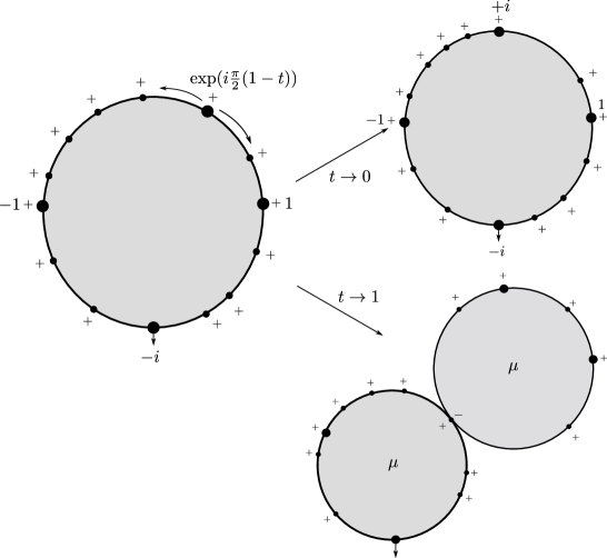
Figure 25. The moduli space $\mathcal{S}^{r,k,l,s}$ and its $t\rightarrow\{0,1\}$ degenerations.

There is an associated Floer operation

(13.30) $$\mathcal{H}_{r,k,l,s}=\mathbf{F}_{\overline{S}^{r,k,l,s}},$$

and we can thus define a morphism of bimodules, of degree -1

(13.31) $$\mathcal{H}\in\hom_{\mathcal{W}\!-\!\mathcal{W}}(\mathcal{W}_{\Delta}\otimes_{\mathcal{W}}\mathcal{W}_{\Delta}\otimes_{\mathcal{W}}\otimes\mathcal{W}_{\Delta},\mathcal{W}_{\Delta}),$$

defined by

(13.32) $$\mathcal{H}^{r|1|s}=\bigoplus_{k,l}\mathcal{H}_{r,k,l,s}.$$

An analysis of the boundaries of the one-dimensional moduli space of maps given by $\overline{\mathcal{S}}_{r,k,l,s}$ reveals

Proposition 13.2.

$\mathcal{H}$ is a chain homotopy between $\mathcal{F}_{\Delta,left,right}$ and $\mu_{LR}$.

Proof.

The $t=1$ strata (13.20) correspond to $\mathcal{F}_{\Delta,left,right}$, the $t=0$ strata (13.21) correspond to $\mu_{LR}$, and the other strata (13.22)-(13.29) correspond to the chain homotopy terms $\mathcal{H}\circ d-d\circ\mathcal{H}$. ∎

13.2. A family of annuli

Recall that the morphism $\mathcal{CY}$ induces functorial maps

(13.33) $$\mathcal{CY}_{\#}:\mathcal{W}_{\Delta}\otimes_{\mathcal{W}\!-\mathcal{W}}\mathcal{W}_{\Delta}\longrightarrow\mathcal{W}_{\Delta}\otimes_{\mathcal{W}\!-\!\mathcal{W}}\mathcal{W}^{!},$$

which, composed with the map

(13.34) $$\bar{\mu}:\mathcal{W}_{\Delta}\otimes_{\mathcal{W}\!-\!\mathcal{W}}\mathcal{W}^{!}\longrightarrow\hom_{\mathcal{W}\!-\!\mathcal{W}}(\mathcal{W}_{\Delta},\mathcal{W}_{\Delta})$$

defined in (2.373), gives a map from (two-pointed) Hochschild homology to Hochschild cohomology. We now prove that this composed map is in fact homotopic to the map from Hochschild homology to cohomology passing through $SH^{*}(M)$.

Theorem 13.1 (Generalized Cardy Condition).

There is a (homotopy)-commutative diagram

(13.35)

We first how this result completes the proof of Theorem 1.1.

Proof of Theorem 1.1.

By Corollary 11.2 and Theorem 1.3, the maps ${}_{2}\mathcal{CO}$ and $\mathcal{CY}_{\#}$ are isomorphisms. Moreover, so is $\bar{\mu}$, by Proposition 2.3 (see also (2.373) for the explicit for of $\bar{\mu}$). Thus by the diagram (13.35), so is ${}_{2}\mathcal{OC}$. By Proposition 5.6, ${}_{2}\mathcal{CO}$ and ${}_{2}\mathcal{OC}$ are homotopic to the usual $\mathcal{CO}$ and $\mathcal{OC}$, implying the result.

Alternatively, let us note that we didn’t need to a priori know that ${}_{2}\mathcal{CO}$ was an isomorphism to conclude the proof. Surjectivity of ${}_{2}\mathcal{OC}$ and injectivity of ${}_{2}\mathcal{CO}$, the contents of Proposition 1.1, suffice. ∎

To construct the homotopy, we introduce some auxiliary moduli spaces of annuli.

Definition 13.3.

The moduli space

(13.36) $$\mathcal{A}_{1}$$

consists of annuli with two positive punctures on the inner boundary, one positive puncture on the outer boundary, and one negative puncture on the outer boundary. The codimension 3 subspace

(13.37) $$\mathcal{A}_{1}^{-}$$

consists of those annuli that are conformally equivalent to

(13.38) $$\{z|1\leq|z|\leq R\}\subset{\mathbb{C}},$$

for any (varying) $R$, with inner positive marked points at $\pm i$, outer positive marked point at $Ri$, and outer negative marked point at $-Ri$.

Definition 13.4.

Define

(13.39) $$\mathcal{A}_{k,l;s,t}$$

to be the moduli space of annuli with

• $k+l+2$ positive marked points on the inner boundary, labeled $a_{0},a_{1},\ldots,a_{k}$, $a_{0}^{\prime},a_{1}^{\prime},\ldots,a_{l}^{\prime}$ in counterclockwise order,

• one negative marked point on the outer boundary, labeled $z_{out}$, and

• $s+t+1$ positive marked points on the outer boundary, labeled counterclockwise from $z_{out}$ as $b_{1},\ldots,b_{s},b_{0}^{\prime},b_{1}^{\prime},\ldots,b_{t}^{\prime}$.

There is a map

(13.40) $$\pi:\mathcal{A}_{k,l;s,t}\longrightarrow\mathcal{A}_{1}$$

given by forgetting all of the marked points except for $a_{0}$, $a_{0}^{\prime}$, $b_{0}^{\prime}$, and $z_{out}$.

Definition 13.5.

Define

(13.41) $$\mathcal{A}_{k,l;s,t}^{-}$$

to be the pre-image of $\mathcal{A}_{1}^{-}$ under $\pi$.

Via the map

(13.42) $$\mathcal{A}_{1}^{-}\longrightarrow(0,1)$$

which associates to any annulus the scaling parameter $\frac{R}{1+R}$, the space $\mathcal{A}_{k,l;s,t}^{-}$ also fibers over $(0,1)$. Compactifying, we see that $\overline{\mathcal{A}}_{k,l;s,t}^{-}$ submerses over $[0,1]$, and has boundary stratum covered by the natural images of the inclusions of the following codimension 1 strata

(13.43) $$\mathcal{R}^{1}_{k,l} \times\mathcal{R}^{1,1}_{s,t}\ \ \ \ \ \ \ \ \ \ \ \ \ \ \ \ \ \ \textrm{(fiber over 1)}$$

(13.44) $$\mathcal{R}_{2}^{s^{\prime},t^{\prime},l^{\prime},k^{\prime}} \times_{(1,1+),(2,3+)}\mathcal{R}^{s-s^{\prime},k-k^{\prime},l-l^{\prime},t-t^{\prime}}\ \ \ \textrm{(fiber over 0)}$$

(13.45) $$\overline{\mathcal{R}}^{k^{\prime}} \times^{a}_{n+1}\overline{\mathcal{A}}_{k-k^{\prime}+1,l;s,t}^{-},\ \ \ 0\leq n<k-k^{\prime}+1$$

(13.46) $$\overline{\mathcal{R}}^{l^{\prime}}\times^{a}_{(n+1)^{\prime}} \times\overline{\mathcal{A}}_{k,l-l^{\prime}+1;s,t}^{-},\ \ \ 0\leq n<l-l^{\prime}+1$$

(13.47) $$\overline{\mathcal{R}}^{k^{\prime}+l^{\prime}+1} \times^{a}_{0}\overline{\mathcal{A}}_{k-k^{\prime},l-l^{\prime};s,t}^{-}$$

(13.48) $$\overline{\mathcal{R}}^{l^{\prime}+k^{\prime}+1} \times^{a}_{0^{\prime}}\overline{\mathcal{A}}_{k-k^{\prime},l-l^{\prime};s,t}^{-}$$

(13.49) $$\overline{\mathcal{R}}^{s^{\prime}} \times^{b}_{n+1}\overline{\mathcal{A}}_{k,l;s-s^{\prime}+1,t}^{-},\ \ \ 0\leq n<s-s^{\prime}+1$$

(13.50) $$\overline{\mathcal{R}}^{t^{\prime}} \times^{b}_{(n+1)^{\prime}}\overline{\mathcal{A}}_{k,l;s,t-t^{\prime}+1}^{-},\ \ \ 0\leq n<t-t^{\prime}+1$$

(13.51) $$\overline{\mathcal{R}}^{s^{\prime}+t^{\prime}+1} \times^{b}_{0^{\prime}}\overline{\mathcal{A}}_{k,l;s-s^{\prime},t-t^{\prime}}^{-}$$

(13.52) $$\overline{\mathcal{A}}_{k,l;s-s^{\prime},t-t^{\prime}}^{-} \times_{s^{\prime}+1}\overline{\mathcal{R}}^{t^{\prime}+s^{\prime}+1}.$$

Here, the notation $\times^{a}_{j}$ means the output of the first stratum is glued to the input point $a_{j}$, $\times^{a}_{j^{\prime}}$ means glue to $a_{j}^{\prime}$, and $\times^{b}_{j}$, $\times^{b}_{j^{\prime}}$ mean the same for $b_{j}$, $b_{j}^{\prime}$. Also, in (13.44), the two special inputs of the first factor and the second special input of the second factor become the special input points on the annulus after gluing. Also, in (13.47) and (13.48), the $k^{\prime}+1$st and $l^{\prime}+1$st marked points of the first component become the special point ($a_{0}$ or $a_{0}^{\prime}$ respectively) after gluing.

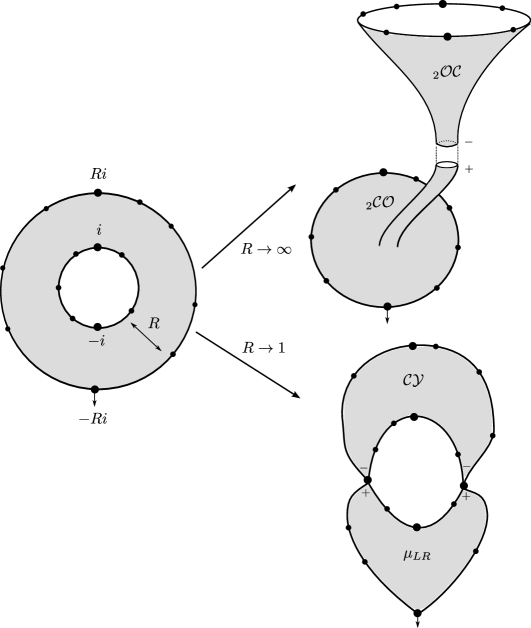
Figure 26. The space of annuli $\mathcal{A}_{k,l;s,t}^{-}$ and its degenerations associated to the endpoints $\{0,1\}$.

Given sign twisting datum

(13.53) $$\vec{t}_{\mathbf{A},k,l,s,t}=\{(1,\ldots,k,k,k+1,\ldots,k+l,k+l,1,\ldots,s,s,s+1,\ldots,s+t,s+t\}$$

with respect to the ordering of boundary inputs

(13.54) $$a_{1},\ldots,a_{k},a_{0}^{\prime},a_{1}^{\prime},\ldots,a_{l}^{\prime},a_{0},b_{1},\ldots,b_{s},z_{in},b_{1}^{\prime},\ldots,b_{t}^{\prime}$$

there are associated Floer operations

(13.55) $$\begin{split}\mathbf{A}_{k,l;s,t}&:=(-1)^{\vec{t}_{\mathbf{A},k,l,s,t}}\mathbf{F}_{\overline{\mathcal{A}}_{k,l;s,t}^{-}}:\\ &(\mathcal{W}_{\Delta}\otimes\mathcal{W}^{\otimes l}\otimes\mathcal{W}_{\Delta}\otimes\mathcal{W}^{\otimes k})^{diag}\otimes\mathcal{W}^{\otimes t}\otimes\mathcal{W}_{\Delta}\otimes\mathcal{W}^{\otimes s}\longrightarrow\mathcal{W}_{\Delta}\end{split}$$

where we have indicated the inputs corresponding to the special points $a_{0}$, $a_{0}^{\prime}$, and $b_{0}^{\prime}$ by the first, second, and third $\mathcal{W}_{\Delta}$ input factor, and the output $z_{out}$ by the output $\mathcal{W}_{\Delta}$ factor. As usual, the $diag$ superscript indicates that the first set of $k+l+2$ inputs must be cyclically composable. Using these operations, define a map

(13.56) $$\mathbf{A}:{{}_{2}}\mathrm{CC}_{*}(\mathcal{W},\mathcal{W})\longrightarrow{{}_{2}}\mathrm{CC}^{*}(\mathcal{W},\mathcal{W})$$

by

(13.57) $$\mathbf{A}:(\mathbf{x}\otimes x_{r}\otimes\cdots\otimes x_{1}\otimes\mathbf{y}\otimes y_{q}\otimes\cdots\otimes y_{1})\longmapsto\Phi$$

where $\Phi$ is the 2-Hochschild co-chain given by

(13.58) $$\begin{split}\Phi(c_{m},\ldots,c_{1},\mathbf{c},d_{n},\ldots,d_{1})=\mathbf{A}_{q,r;n,m}(&\mathbf{x}\otimes x_{r}\otimes\cdots\otimes x_{1}\otimes\mathbf{y}\\ &\otimes y_{q}\otimes\cdots\otimes y_{q};c_{m},\ldots,c_{1},\mathbf{c},d_{n},\ldots,d_{1}).\end{split}$$

A dimension computation shows that the operation $\mathbf{A}$ has degree $n-1$ as a map from Hochschild homology to Hochschild cohomology. An analysis of the boundary of the one-dimensional moduli spaces of maps with source domain the various $\mathcal{A}_{k,l;s,t}^{-}$ reveals:

Proposition 13.3.

$\mathbf{A}$ gives a chain homotopy between ${{}_{2}}\mathcal{CO}\circ{{}_{2}}\mathcal{OC}$ and $\mu_{LR}\circ\mathcal{CY}_{\#}$.

Proof.

The strata over the endpoints of the interval $\{0,1\}$ correspond exactly to the operations ${{}_{2}}\mathcal{CO}\circ{{}_{2}}\mathcal{OC}$ and $\mu_{LR}\circ\mathcal{CY}_{\#}$. The various intermediate strata give terms corresponding to $d_{\mathrm{CC}^{*}}\circ\mathbf{A}\pm\mathbf{A}\circ d_{\mathrm{CC}_{*}}$. In Appendix B we discuss the ingredients necessary to check the signs of this equation. ∎

By postcomposing with the chain homotopy in Proposition 13.2 between $\bar{\mu}$ and $\mu_{LR}$, Theorem 13.1 follows.

Remark 13.1.

If bimodules $\mathcal{B}_{0},\mathcal{B}_{1}$ come from any Lagrangian in the product for which we are able to define the quilt functor,

(13.59) $$\begin{split}\mathcal{B}_{0}&=\mathbf{M}(L_{0})\\ \mathcal{B}_{1}&=\mathbf{M}(L_{1})\end{split}$$

then there is an analogue of the Cardy condition, which looks like (13.35):

(13.60)

Here, $\mathcal{B}_{0}^{!}$ is the bimodule dual of $\mathcal{B}_{0}$, as defined in Section 2.13, and $\mathcal{CY}^{\mathcal{B}_{0}}$ is a generalization of our $\mathcal{CY}$ morphism. The moduli space controlling the relevant commutative diagram is a quilted generalization of the annulus. The only obstacle to the existence of this diagram for arbitrary pairs of Lagrangians in $M^{2}$ is our current inability to define the functor $\mathbf{M}$ in complete generality, due to issues of admissibility and compactness of moduli spaces in $M^{2}$.

14. Some consequences

14.1. A converse result

In Section 11, we proved that if $M$ is non-degenerate, then the product Lagrangians $L_{i}\times L_{j}$ split-generate $\Delta$ in $\mathcal{W}^{2}$. The proof went via analyzing a homotopy commutative diagram

(14.1) $$\lx@xy@svg{\hbox{\raise 0.0pt\hbox{\kern 28.57782pt\hbox{\ignorespaces\ignorespaces\ignorespaces\hbox{\vtop{\kern 0.0pt\offinterlineskip\halign{\entry@#!@&&\entry@@#!@\cr&\\&\crcr}}}\ignorespaces{\hbox{\kern-28.57782pt\raise 0.0pt\hbox{\hbox{\kern 0.0pt\raise 0.0pt\hbox{\hbox{\kern 3.0pt\raise 0.0pt\hbox{$\textstyle{{}_{2}\mathrm{CC}_{*}(\mathcal{W},\mathcal{W})\ignorespaces\ignorespaces\ignorespaces\ignorespaces\ignorespaces\ignorespaces\ignorespaces\ignorespaces}$}}}}}}}\ignorespaces\ignorespaces\ignorespaces\ignorespaces{}{\hbox{\lx@xy@droprule}}\ignorespaces\ignorespaces\ignorespaces{\hbox{\kern 30.80699pt\raise 5.39166pt\hbox{{}\hbox{\kern 0.0pt\raise 0.0pt\hbox{\hbox{\kern 3.0pt\hbox{\hbox{\kern 0.0pt\raise-2.39166pt\hbox{$\scriptstyle{\Gamma\ \ \ }$}}}\kern 3.0pt}}}}}}\ignorespaces{\hbox{\kern 62.84627pt\raise 0.0pt\hbox{\hbox{\kern 0.0pt\raise 0.0pt\hbox{\lx@xy@tip{1}\lx@xy@tip{-1}}}}}}{\hbox{\lx@xy@droprule}}{\hbox{\lx@xy@droprule}}\ignorespaces\ignorespaces\ignorespaces\ignorespaces{}{\hbox{\lx@xy@droprule}}\ignorespaces\ignorespaces\ignorespaces{\hbox{\kern 0.0pt\raise-21.36401pt\hbox{{}\hbox{\kern 0.0pt\raise 0.0pt\hbox{\hbox{\kern 3.0pt\hbox{\hbox{\kern 0.0pt\raise-1.74722pt\hbox{$\scriptstyle{{}_{2}\mathcal{OC}}$}}}\kern 3.0pt}}}}}}\ignorespaces{\hbox{\kern 0.0pt\raise-31.59193pt\hbox{\hbox{\kern 0.0pt\raise 0.0pt\hbox{\lx@xy@tip{1}\lx@xy@tip{-1}}}}}}{\hbox{\lx@xy@droprule}}{\hbox{\lx@xy@droprule}}{\hbox{\kern 62.84627pt\raise 0.0pt\hbox{\hbox{\kern 0.0pt\raise 0.0pt\hbox{\hbox{\kern 3.0pt\raise 0.0pt\hbox{$\textstyle{\mathcal{Y}^{r}_{\Delta}\otimes_{\tilde{\mathcal{W}}^{2}_{split}}\mathcal{Y}^{l}_{\Delta}\ignorespaces\ignorespaces\ignorespaces\ignorespaces}$}}}}}}}\ignorespaces\ignorespaces\ignorespaces\ignorespaces{}{\hbox{\lx@xy@droprule}}\ignorespaces\ignorespaces\ignorespaces{\hbox{\kern 82.48898pt\raise-21.36401pt\hbox{{}\hbox{\kern 0.0pt\raise 0.0pt\hbox{\hbox{\kern 3.0pt\hbox{\hbox{\kern 0.0pt\raise-0.8264pt\hbox{$\scriptstyle{\mu}$}}}\kern 3.0pt}}}}}}\ignorespaces{\hbox{\kern 82.48898pt\raise-32.22803pt\hbox{\hbox{\kern 0.0pt\raise 0.0pt\hbox{\lx@xy@tip{1}\lx@xy@tip{-1}}}}}}{\hbox{\lx@xy@droprule}}{\hbox{\lx@xy@droprule}}{\hbox{\kern-22.17845pt\raise-42.72803pt\hbox{\hbox{\kern 0.0pt\raise 0.0pt\hbox{\hbox{\kern 3.0pt\raise 0.0pt\hbox{$\textstyle{CH^{*}(M)\ignorespaces\ignorespaces\ignorespaces\ignorespaces}$}}}}}}}\ignorespaces\ignorespaces\ignorespaces\ignorespaces{}{\hbox{\lx@xy@droprule}}\ignorespaces\ignorespaces\ignorespaces{\hbox{\kern 35.24957pt\raise-37.33636pt\hbox{{}\hbox{\kern 0.0pt\raise 0.0pt\hbox{\hbox{\kern 3.0pt\hbox{\hbox{\kern 0.0pt\raise-2.39166pt\hbox{$\scriptstyle{D}$}}}\kern 3.0pt}}}}}}\ignorespaces{\hbox{\kern 52.57782pt\raise-42.72803pt\hbox{\hbox{\kern 0.0pt\raise 0.0pt\hbox{\lx@xy@tip{1}\lx@xy@tip{-1}}}}}}{\hbox{\lx@xy@droprule}}{\hbox{\lx@xy@droprule}}{\hbox{\kern 52.57782pt\raise-42.72803pt\hbox{\hbox{\kern 0.0pt\raise 0.0pt\hbox{\hbox{\kern 3.0pt\raise 0.0pt\hbox{$\textstyle{\hom_{\tilde{\mathcal{W}}^{2}}(\Delta,\Delta)}$}}}}}}}\ignorespaces}}}}\ignorespaces, \textstyle{{}_{2}\mathrm{CC}_{*}(\mathcal{W},\mathcal{W})\ignorespaces\ignorespaces\ignorespaces\ignorespaces\ignorespaces\ignorespaces\ignorespaces\ignorespaces} \scriptstyle{\Gamma\ \ \ } \scriptstyle{{}_{2}\mathcal{OC}} \textstyle{\mathcal{Y}^{r}_{\Delta}\otimes_{\tilde{\mathcal{W}}^{2}_{split}}\mathcal{Y}^{l}_{\Delta}\ignorespaces\ignorespaces\ignorespaces\ignorespaces} \scriptstyle{\mu} \textstyle{CH^{*}(M)\ignorespaces\ignorespaces\ignorespaces\ignorespaces} \scriptstyle{D} \textstyle{\hom_{\tilde{\mathcal{W}}^{2}}(\Delta,\Delta)} \textstyle{{}_{2}\mathrm{CC}_{*}(\mathcal{W},\mathcal{W})\ignorespaces\ignorespaces\ignorespaces\ignorespaces\ignorespaces\ignorespaces\ignorespaces\ignorespaces} \scriptstyle{\Gamma\ \ \ } \scriptstyle{{}_{2}\mathcal{OC}} \textstyle{\mathcal{Y}^{r}_{\Delta}\otimes_{\tilde{\mathcal{W}}^{2}_{split}}\mathcal{Y}^{l}_{\Delta}\ignorespaces\ignorespaces\ignorespaces\ignorespaces} \scriptstyle{\mu} \textstyle{CH^{*}(M)\ignorespaces\ignorespaces\ignorespaces\ignorespaces} \scriptstyle{D} \textstyle{\hom_{\tilde{\mathcal{W}}^{2}}(\Delta,\Delta)}$$

where $\tilde{\mathcal{W}}_{split}^{2}$ was a category quasi-isomorphic to $\mathcal{W}^{2}_{split}$, the full subcategory of product Lagrangians in $\mathcal{W}^{2}$.

Corollary 14.1.

Under the same hypotheses, $\Gamma$ is a quasi-isomorphism.

Proof.

The map $H^{*}(\mu)$ hits the unit, so by Proposition 2.7 $H^{*}(\mu)$ is an isomorphism. $D$ is an isomorphism by definition, and we then note, thanks to Theorem 1.4, that ${}_{2}\mathcal{OC}$ is also a quasi-isomorphism. Hence, $\Gamma$ is a quasi-isomorphism. ∎

Remark 14.1.

It seems believable that the map $\Gamma$ is always an isomorphism, via the existence of an explicit quasi-inverse instead of such circuitous arguments. At the time of writing we have not come up with a simple proof.

With the technology we have established, we can also see that non-degeneracy is in fact equivalent to split-generation of the diagonal:

Proposition 14.1.

If $\Delta$ is split-generated by product Lagrangians in $\mathcal{W}^{2}$, then $M$ is non-degenerate.

Proof.

If so, then since the quilt functor $\mathbf{M}$ is full on product Lagrangians (Proposition 9.5), we conclude that $\mathbf{M}$ is full on $\Delta$. This implies that the maps $\mathcal{CY}_{\#}$, $\bar{\mu}$, and $\mathcal{CO}$ are isomorphisms in the Cardy Condition diagram (1.13) (this is the content of Corollary 12.1, Corollary 2.3, and Proposition 9.7). Hence $\mathcal{OC}$ is an isomorphism as well; in particular, it hits the unit. ∎

In particular, $\Gamma$ is once more an isomorphism.

14.2. The fundamental class

Assume $M$ is non-degenerate, and let $\sigma\in\mathrm{CC}_{*}(\mathcal{W},\mathcal{W})$ be any pre-image of $[e]\in SH^{*}(M)$ under the map $\mathcal{OC}$. Because $\mathcal{OC}$ is of degree $n$, $\sigma$ is a degree $-n$ element. Following terminology from the introduction, call $\sigma$ a fundamental class for the wrapped Fukaya category. Our reason for this terminology is that

Corollary 14.2.

Cap product with $\sigma$ induces an isomorphism

(14.2) $$\cdot\cap\sigma:\mathrm{HH}^{*}(\mathcal{W},\mathcal{W})\stackrel{{\scriptstyle\sim}}{{\longrightarrow}}\mathrm{HH}_{*-n}(\mathcal{W},\mathcal{W})$$

that is quasi-inverse to the geometric morphisms $\mathcal{CO}\circ\mathcal{OC}$. Thus, by Theorem 1.4, it is also quasi-inverse to $\mu_{LR}\circ\mathcal{CY}_{\#}$.

Proof.

We note that by the module structure compatibility of $\mathcal{OC}$ the following holds on the level of homology:

(14.3) $$\begin{split}\mathcal{OC}((\mathcal{CO}\circ\mathcal{OC}(x))\cap\sigma)&=\mathcal{OC}(x)\cdot\mathcal{OC}(\sigma)\\ &=\mathcal{OC}(x)\cdot[e]\\ &=\mathcal{OC}(x).\end{split}$$

Since $\mathcal{OC}$ is a homology-level isomorphism, we conclude that

(14.4) $$(\mathcal{CO}\circ\mathcal{OC}(x))\cap\sigma=x$$

as desired. ∎

14.3. A ring structure on Hochschild homology

We can pull back the ring structure from Hochschild cohomology to Hochschild homology. Thanks to Theorem 1.4, this can be done without passing through symplectic cohomology.

Corollary 14.3.

Let $\sigma$ be the pre-image of the unit, and let $\alpha$, $\beta$ be two classes in $\mathrm{HH}_{*}(\mathcal{W},\mathcal{W})$ that map to elements $a$ and $b$ of symplectic cohomology via $\mathcal{OC}$. Then, the following Hochschild homology classes are equal in homology and map to $a\cdot b$:

(14.5) $$\alpha\star^{1}\beta :=(\bar{\mu}\circ\mathcal{CY}_{\#}(\alpha))\cap\beta$$

(14.6) $$\alpha\star^{2}\beta :=\alpha\cap(\bar{\mu}\circ\mathcal{CY}_{\#}(\beta))$$

(14.7) $$\alpha\star^{3}\beta :=\left((\bar{\mu}\circ\mathcal{CY}_{\#})(\alpha)*(\bar{\mu}\circ\mathcal{CY}_{\#})(\beta)\right)\cap\sigma.$$

It is illustrative to write down an explicit expression for (14.5) in terms of operations. First, we note that for two-pointed complexes, cap-product has a very simple form

(14.8) $$\begin{split}{{}_{2}}\mathrm{CC}_{*}(\mathcal{W},\mathcal{W})\times{{}_{2}}\mathrm{CC}^{*}(\mathcal{W},\mathcal{W})&\longrightarrow{{}_{2}}\mathrm{CC}_{*}(\mathcal{W},\mathcal{W})\\ (\alpha,\mathcal{F})&\longmapsto\mathcal{F}_{\#}(\alpha)\end{split}$$

where $\mathcal{F}_{\#}$ is the pushforward operation on the tensor product $\mathcal{W}_{\Delta}\otimes_{\mathcal{W}\!-\!\mathcal{W}}\mathcal{W}_{\Delta}$ that acts by collapsing terms around and including the first factor of $\mathcal{W}_{\Delta}$ (with usual Koszul reordering signs).

Now, if $\beta$ is the Hochschild class represented by

(14.9) $$\beta=\mathbf{a}\otimes b_{1}\otimes\cdots\otimes b_{t}\otimes\mathbf{b}\otimes a_{1}\otimes\cdots\otimes a_{s}$$

and $\alpha$ is represented by

(14.10) $$\alpha=\mathbf{c}\otimes c_{1}\otimes\cdots\otimes c_{v}\otimes\mathbf{d}\otimes d_{1}\otimes\cdots\otimes d_{w}$$

then the formula (14.5) is, up to sign:

(14.11) $$\begin{split}\alpha\star^{1}\beta:=\sum\bigg{(}\bigg{(}\mu_{\mathcal{W}}(&a_{s-k^{\prime\prime}+1},\ldots,a_{s-k^{\prime}},\cdot,c_{r^{\prime}+1},\ldots,c_{r^{\prime\prime}-1},\\ &\mu_{\mathcal{W}}(c_{r^{\prime\prime}},\ldots,c_{v}\mathbf{d},d_{1},\ldots,d_{w-q^{\prime}},\cdot,b_{l^{\prime}+1},\ldots,b_{l^{\prime}+l^{\prime\prime}}),\\ &\ \ \ \ \ \ b_{l^{\prime}+l^{\prime\prime}+1},\ldots,b_{l^{\prime}+l^{\prime\prime}+l^{\prime\prime\prime}}\bigg{)}\\ &\circ\mathcal{CY}_{k^{\prime},l^{\prime},q^{\prime},r^{\prime}}(d_{w-q^{\prime}+1},\ldots,d_{w},\mathbf{c},c_{1},\ldots,c_{r}^{\prime};\\ &\ \ \ \ \ \ \ a_{s-k^{\prime}+1},\ldots,a_{s},\mathbf{a},b_{1},\ldots,b_{l}^{\prime})\bigg{)}\\ &\otimes b_{l^{\prime}+l^{\prime\prime}+l^{\prime\prime\prime}+1}\otimes\cdots\otimes b_{t}\otimes\mathbf{b}\otimes a_{1}\otimes\cdots a_{s-k^{\prime\prime}}.\end{split}$$

This formula is formally analogous to Bourgeois, Ekholm, and Eliashberg’s surgery formula for the symplectic cohomology product on a Weinstein manifold [BEE2], which is expressed as sums over operations similar to $\mathcal{CY}$ and $\mu_{\mathcal{W}}$ applied to Legendrian symplectic field theory invariants of attaching cores. A detailed comparison between these formulae, in the case that our essential collection of Lagrangians are the ascending co-cores of a Weinstein manifold, will appear elsewhere.

Appendix A Action, energy and compactness

The goal of this appendix is to prove a compactness result for Floer-theoretic operations controlled by bordered Riemann surfaces mapping into a Liouville manifold, under some assumptions about the almost complex structure and Hamiltonian perturbation terms. There are several existing compactness results for the wrapped Fukaya category and some open-closed maps, e.g. [Abouzaid:2010kx]*§B, which are unfortunately not directly applicable for our choices of Hamiltonian perturbations. The problems occur because we use time-dependent perturbations of a standard Hamiltonian, which we cannot guarantee will vanish at infinitely many levels of the cylindrical coordinate $r$ (this is an essential assumption in [Abouzaid:2010kx]*§B). Solutions to Floer’s equation for such perturbed Hamiltonians will fail to satisfy a maximum principle, but if the complex structure has been carefully chosen and the time-dependent perturbations are sufficiently small, this failure can be controlled. We make use in an essential way of a delicate technique for obtaining a-priori $C^{0}$ bounds on such solutions due to Floer-Hofer and Cieliebak [Floer:1994uq] [Cieliebak:1994fk]. This technique has also been used by Oancea [Oancea:2008fk], whose work we draw upon.

Remark A.1.

Our situation is a little different from [Floer:1994uq] [Cieliebak:1994fk] [Oancea:2008fk] in that we need a variant of their compactness result for potentially finite cylindrical regions in a larger Riemann surface. This, and differing conventions regarding Hamiltonians (quadratic versus linear) and complex structures (contact type versus rescaled contact type) prevent us from citing any of these papers directly.

Our setup is as follows: Let $W$ be a Liouville manifold with cylindrical end

(A.1) $$W=\bar{W}\cup_{\partial W}\partial W\times[1,\infty)_{r}.$$

The coordinate on the end is given by a function $\pi_{r}$ on $W-\bar{W}$, which we extend over the interior of $W$ to a function

(A.2) $$\pi_{r}:W\longrightarrow[0,\infty)$$

such that

(A.3) $$\bar{W}=\pi^{-1}([0,1]).$$

Let $S$ be a bordered surface with boundary $\partial S$, and equip $S$ with a Floer datum in the sense of Definition 4.11, namely:

• a collection of $\delta$-bounded weighted strip and cylinder data,

• a sub-closed one form $\alpha_{S}$, compatible with the weighted strip and cylinder data

• a primary Hamiltonian $H_{S}:S\rightarrow\mathcal{H}(M)$ that is $H$ compatible with the weighted strip and cylinder data

• an adapted rescaling function $a_{S}$, constant and equal to the weights on each strip and cylinder region,

• an almost complex structure $J_{S}$ that is adapted to the weighted strip and cylinder data, the rescaling function $a_{S}$, and some fixed $J_{t}$, and

• an $S^{1}$ perturbation $F_{S}$ adapted to $(F_{T},\phi_{\epsilon})$ for some $F_{T}$, $\phi_{\epsilon}$ as in the definition.

Remark A.2.

The requirement that $S$ carry a sub-closed one form with asymptotics specified above implies via Stokes theorem that $S$ must have at least one output marked point. Although the use of the sub-closed one form may seem like a technical artifice of the proofs of compactness here and elsewhere, this constraint on $S$ is an essential one. Indeed, symplectic cohomology and morphism spaces in the wrapped category are often infinite dimension, and thus cannot admit the Poincaré duality type pairings that arise from surfaces without outputs.

Fix a Lagrangian labeling $\vec{L}$ for the boundary components of $S$ and a compatible choice of input and output chords and orbits corresponding to the positive and negative marked points on $S$

(A.4) $$\begin{split}\vec{x}_{in},\vec{x}_{out},\vec{y}_{in},\vec{y}_{out}.\end{split}$$

We study maps $u:S\rightarrow W$ satisfying Floer’s equation for this datum, namely

(A.5) $$(du-X_{S}\otimes\gamma)^{0,1}=0$$

with asymptotic/boundary conditions

$$\begin{cases}\lim_{p\rightarrow z^{\pm}_{k}}u=y_{k}^{\pm}\\ \lim_{p\rightarrow b^{\pm}_{j}}u=x_{j}^{\pm}\\ \mathrm{for\ }p\in\partial^{n}S,&u(p)\in\psi^{\rho(p)}(L_{n})\end{cases}.$$

Here $X_{S}$ is the Hamiltonian vector field corresponding to the total Hamiltonian

(A.6) $$H^{tot}_{S}=H_{S}+F_{S}.$$

The compactness result we need is:

Theorem A.1.

Given such a map $u:S\rightarrow W$, there is a constant $C$ depending only on $F_{t}$, and $\phi_{\epsilon}$, $\vec{x}_{in}$, $\vec{x}_{out}$, $\vec{y}_{in}$, $\vec{y}_{out}$ such that

(A.7) $$(\pi_{r}\circ u)\leq C.$$

Moreover, given any set of $\vec{y}_{in}$ $\vec{x}_{in}$, there are a finite number of collections $\vec{y}_{out}$, $\vec{x}_{out}$ for which the relevant moduli spaces are non-empty.

First, we define appropriate notions of action and energy. Suppose we have fixed a Hamiltonian $H$ and a time-dependent perturbation $F_{t}$, and have picked a surface $S$ with compatible Floer data. Let $x\in\chi(L_{i},L_{j})$ be the asymptotic condition at strip-like end $\epsilon^{k}$ with corresponding weight $w_{k}$. Moreover, suppose the perturbation term $F_{S}$ is equal to the constant $C_{k}$ on this strip-like end (this can be chosen to be zero if there are no interior marked points in $S$).

Definition A.1.

The action of $x$ is defined to be the quantity

(A.8) $$\mathcal{A}(x):=-\int_{0}^{1}(\tilde{x}_{w_{k}})^{*}\theta+\int_{0}^{1}w_{k}\cdot H^{w_{k}}(x(t))dt+f_{L_{j}}(x(1))-f_{L_{i}}(x(0))+w_{k}C_{k}.$$

where the $f_{L_{i}}$ are the chosen fixed primitives of the Lagrangians $L_{i}$,

(A.9) $$H^{w_{k}}:=\frac{(\psi^{w_{k}})^{*}H}{w_{k}^{2}},$$

and

(A.10) $$\tilde{x}_{w_{k}}$$

is the chord $x$ thought of as a time-1 chord of $w_{k}\cdot H^{w_{k}}$, under the rescaling correspondence (4.3).

Similarly, let $y\in\mathcal{O}$ be the asymptotic condition at cylindrical end $\delta^{l}$ with corresponding weight $v_{l}$.

Definition A.2.

The action of $y$ is the quantity

(A.11) $$\mathcal{A}(y):=-\int_{S^{1}}(\tilde{y}_{v_{l}})^{*}\theta+\int_{0}^{1}v_{l}\cdot H^{v_{l}}(x(t))dt+\int_{0}^{1}v_{l}\cdot F_{t}^{v_{l}}(t,x(t))dt$$

where $H^{v_{l}}$ is as before and $F_{t}^{v_{l}}$ is defined as

(A.12) $$F_{t}^{v}:=\frac{(\psi^{v_{l}})^{*}F_{t}}{v_{l}^{2}}.$$

Lemma A.1.

The action of a Hamiltonian chord or orbit becomes arbitrarily negative as $r\rightarrow\infty$.

Proof.

This Lemma is a variant of one in [Abouzaid:2010kx, §B.2]. The first observation is, by Lemma 4.1, that

(A.13) $$H^{w_{k}}=H=r^{2}$$

away from a compact subset. Also, for a Hamiltonian chord $\tilde{x}_{w_{k}}$

(A.14) $$\begin{split}\tilde{x}_{w_{k}}^{*}\theta&=\theta(X_{w_{k}\cdot H^{w_{k}}})dt\\ &=w_{k}\cdot\omega(Z,X_{H^{w_{k}}})dt\\ &=w_{k}\cdot dH^{w_{k}}(Z)dt\\ &=2w_{k}\cdot rdr(r\partial_{r})dt\\ &=2w_{k}r^{2}dt.\end{split}$$

Thus, for a chord $x\in\chi(L_{i},L_{j})$ away from a compact set (so $f_{L_{j}}$ and $f_{L_{i}}$ are zero):

(A.15) $$\mathcal{A}(x) =-\int_{0}^{1}{\tilde{x}_{w_{k}}}^{*}\theta+\int_{0}^{1}w_{k}H^{w_{k}}(x(t))dt+w_{k}C_{k}$$

(A.16) $$=-\int_{0}^{1}w_{k}\cdot r^{2}dt+w_{k}C_{k},$$

which satisfies the Lemma. Similarly for an orbit $y\in\mathcal{O}$,

(A.17) $$\mathcal{A}(y) =-\int_{0}^{1}\tilde{y}_{v_{l}}^{*}\theta+\int_{0}^{1}v_{l}\cdot H_{S}(t,y(t))dt$$

(A.18) $$=-\int_{0}^{1}v_{l}\cdot(\theta(X_{H^{v_{l}}})+\theta(X_{F^{v_{l}}})-H^{v_{l}}-F^{v_{l}})dt$$

(A.19) $$=-\int_{0}^{1}v_{l}\cdot(H^{v_{l}}+\theta(X_{F^{v_{l}}})-F^{v_{l}})dt.$$

The above expression also satisfies the Lemma, as $H^{v_{l}}$ dominates $\theta(X_{F^{v_{l}}})$ and $F^{v_{l}}$ away from a compact set. ∎

Following [Abouzaid:2010ly], given a map $u$ satisfying Floer’s equation, we define two notions of energy. The geometric energy of $u$ is defined as

(A.20) $$E_{geo}(u):=\int_{S}||du-X\otimes\gamma||^{2}.$$

where the norm $||\cdot||$ comes from the complex structure $J_{S}$. Picking local coordinates $z=s+it$ for $S$, we see that for a solution $u$ to Floer’s equation,

(A.21) $$\begin{split}E_{geo}(u)&=\int\omega((du-X\otimes\gamma)(\partial_{s}),J_{S}(du-X\otimes\gamma)(\partial_{s})dsdt\\ &=\int\omega(du(\partial_{s})-X\otimes\gamma(\partial_{s}),(du-X\otimes\gamma)\circ j(\partial_{s}))dsdt\\ &=\int_{S}\left(\omega(\partial_{s}u,\partial_{t}u)-\omega(X\otimes\gamma(\partial_{s}),\partial_{t}u)-\omega(\partial_{s}u,X\otimes\gamma(\partial_{t}))\right)dsdt\\ &=\int_{S}\left(u^{*}\omega-(dH(\partial_{s}u)\gamma(\partial_{t})-dH(\partial_{t}u)\gamma(\partial_{s}))dsdt\right)\\ &=\int_{S}u^{*}\omega-d(u^{*}H)\gamma,\end{split}$$

a version of the energy identity for $J$-holomorphic curves. The topological energy of $u$ is defined as

(A.22) $$E_{top}(u):=\int_{S}u^{*}\omega-\int_{S}d(u^{*}(H_{S})\cdot\gamma).$$

Since $\gamma$ is sub-closed and $H_{S}$ is positive,

(A.23) $$0\leq E_{geo}(u)\leq E_{top}(u).$$

Noting that

(A.24) $$\epsilon_{k}^{*}(u^{*}H_{S}\gamma)=w_{k}\cdot(H^{w_{k}}+C_{k})dt$$

on strip-like ends and

(A.25) $$\delta_{l}^{*}(u^{*}H_{S}\gamma)=(w_{k}\cdot H^{v_{l}}+F_{T}^{v_{l}})dt$$

on cylindrical ends, we apply Stokes’ theorem to (A.22) to conclude:

(A.26) $$E_{top}(u)=(\sum_{y\in\vec{y}_{out}}\mathcal{A}(y)-\sum_{y\in\vec{y}_{in}}\mathcal{A}(y))+(\sum_{x\in\vec{x}_{out}}\mathcal{A}(x)-\sum_{x\in\vec{x}_{in}}\mathcal{A}(x)).$$

Proposition A.1.

For any $x_{in}$, $y_{in}$, there are finitely many choices of $x_{out}$, $y_{out}$ such that there is a solution $u$ to the relevant Floer’s equation.

Proof.

By Lemma A.1 and (A.26), for fixed inputs $\vec{x}_{in}$, $\vec{y}_{in}$, for all but a finite selection of $\vec{x}_{out}$, $\vec{y}_{out}$, any $u$ satisfying Floer’s equation with asymptotic conditions $(\vec{x}_{in},\vec{y}_{in},\vec{x}_{out},\vec{y}_{out})$ has negative $E_{geo}(u)$, which is impossible. ∎

Given a map

(A.27) $$u:S\longrightarrow W$$

as above, there is a notion of intermediate action of $u$ along a loop $S^{1}\hookrightarrow S$.

Definition A.3.

Define the intermediate action of an embedded oriented loop $\mathcal{L}:S^{1}\rightarrow S$ to be:

(A.28) $$\mathcal{A}(\mathcal{L}):=-\int_{S^{1}}\mathcal{L}^{*}u^{*}\theta+\int_{S^{1}}\mathcal{L}^{*}(u^{*}(H_{S}\cdot\gamma))$$

A useful fact about intermediate action is:

Lemma A.2.

There are constants $c_{1}$, $c_{2}$ depending on the input and output chords and orbits such that

(A.29) $$\mathcal{A}(\mathcal{L})\in[c_{1},c_{2}]$$

for any embedded oriented loop $\mathcal{L}$.

Proof.

As $S$ is genus 0, any embedded loop $\mathcal{L}$ is separates $S$ into two regions, one $S_{in}$ that has outgoing boundary on $\mathcal{L}$ and one $S_{out}$ that has incoming boundary on $\mathcal{L}$. We note that topological energy $E_{top}(u)$ is non-negative on any sub-region of $S$ and additive, i.e.

(A.30) $$E_{top}(u)=E_{top}(u|_{S_{in}})+E_{top}(u|_{S_{out}}),\ E_{top}(u|_{S_{in}}),E_{top}(u|_{S_{out}})\geq 0.$$

Hence

(A.31) $$\begin{split}E_{top}(u|_{S_{out}})&\leq E_{top}(u)\\ E_{top}(u|_{S_{in}})&\leq E_{top}(u).\end{split}$$

Now each of $E_{top}(u|_{S_{out}})$, $E_{top}(u|_{S_{in}})$ can be expressed via Stokes theorem as the positive or negative action of $\mathcal{L}$ respectively plus/minus actions of inputs and outputs on each of $S_{out}$/$S_{in}$, so we obtain upper and lower bounds for $\mathcal{A}(\mathcal{L})$ in terms of actions of inputs and outputs. ∎

Now, given a fixed Floer datum on $S$, we view $S$ as the union of two regions with different Hamiltonian behavior. On the first region, there is a non-zero time-dependent perturbation:

Definition A.4.

Define the cylindrical perturbed regions $S^{c}$ of $S$ to be the union of the images of the

• cylindrical ends

  $$\delta_{\pm}^{j}:A_{\pm}\longrightarrow S,$$

  and

• finite cylinders

  $$\delta^{r}:[a_{r},b_{r}]\times S^{1}\longrightarrow S$$

in the strip and cylinder data chosen for $S$.

Recall that the Floer datum on $S$ consists of $\delta$-bounded cylinder data, and an $S^{1}$ perturbation adapted to $(F_{T},\phi_{\epsilon})$, for some chosen $\delta\ll 1$ and $\epsilon\ll 1$, the sense of Definitions 4.4 and 4.10. This implies that on the $\bar{\delta}$-collar (see Definition 4.5)

(A.32) $$S^{\bar{\delta}}$$

of $S$, with

(A.33) $$\bar{\delta}=\delta\cdot\epsilon,$$

the perturbation $F_{T}$ is locally constant.

Definition A.5.

Define the unperturbed region $S^{u}$ of $S$ to be the union of the complement of the cylindrical perturbed region $S\backslash S^{c}$ with the $\bar{\delta}$-collar $S^{\bar{\delta}}$. This is the region where the perturbation term $F_{T}$ is locally constant.

The intersection of the two regions $S^{u}$ and $S^{c}$ is exactly the $\bar{\delta}$ collar $S^{\bar{\delta}}$.

We now examine the function

(A.34) $$\rho=\pi_{r}\circ u$$

on each of the two regions of $S$, $S^{u}$ and $S^{c}$. In the next two sections, we prove the following claims:

Proposition A.2.

A maximum principle holds for $\rho$ on the unperturbed region $S^{u}$.

Proposition A.3.

On the portion of the cylindrical perturbed region $S^{c}$ outside the $\bar{\delta}$-collar

(A.35) $$S^{c}\backslash S^{\bar{\delta}}$$

there is an upper bound on $\rho$ in terms of the Floer data and asymptotic conditions.

Remark A.3.

Note that we are only able to directly establish direct upper bounds for $\rho$ outside of a collar of $S^{c}$, and are forced to rely on the maximum principle to deduce bounds for $\rho$ on the collar. This has to do with the technique used to establish such bounds.

These results, along with Proposition A.1 imply Theorem A.1.

A.1. The unperturbed region

In a portion of the unperturbed region $S^{u}$ mapping to the conical end of $W$, the total Hamiltonian is given by $H_{S}$, a quadratic function, plus a locally constant function $F_{S}$. Thus, the Hamiltonian vector field $X_{S}$ is equal to

(A.36) $$X_{S}=2r\cdot R,$$

where $R$ is the Reeb flow on $\partial W$. In particular,

(A.37) $$dr(X)=0.$$

Recall that on the conical end, our (surface-dependent) almost complex structure $J_{S}$ satisfies

(A.38) $$dr\circ J=\frac{a_{S}}{r}\cdot\theta$$

for some positive rescaling function $a_{S}:S\rightarrow[1,\infty)$. Namely, setting

(A.39) $$\mathcal{S}:=\frac{1}{2}r^{2}$$

we have that

(A.40) $$d\mathcal{S}\circ J=rdr\circ J=a_{s}\cdot\theta.$$

Now, consider Floer’s equation on the conical end

(A.41) $$J\circ(du-X\otimes\gamma)=(du-X\otimes\gamma)\circ j$$

and apply $d\mathcal{S}$ to both sides, with $\xi=\mathcal{S}\circ u=\frac{1}{2}\rho^{2}$ to obtain

(A.42) $$d^{c}\xi=-a_{S}\cdot(\theta\circ(du-X\otimes\gamma))$$

Differentiating once more,

(A.43) $$\begin{split}dd^{c}\xi=-a_{S}(u^{*}\omega-d(\theta(X)\cdot\gamma))-da_{S}\wedge(\theta\circ(du-X\otimes\gamma)).\end{split}$$

Substituting (A.42) into (A.43), we finally obtain the following second-order differential equation for $\xi$:

(A.44) $$dd^{c}\xi=-a_{S}(u^{*}\omega-d(\theta(X)\cdot\gamma))+\frac{da_{S}}{a_{S}}\wedge d^{c}\xi$$

On the cylindrical end, we have that up to a locally constant function

(A.45) $$\theta(X)=2r^{2}=2H;$$

hence

(A.46) $$\begin{split}u^{*}\omega-d(\theta(X)\cdot\gamma)&=u^{*}\omega-d(\theta(X))\wedge\gamma-\theta(X)d\gamma\\ &=u^{*}\omega-2d(u^{*}H)\wedge\gamma-\theta(X)d\gamma\\ &=(u^{*}\omega-d(u^{*}H)\wedge\gamma)+\theta(X)d\gamma-d(u^{*}H)\wedge\gamma\\ &=(u^{*}\omega-d(u^{*}H)\wedge\gamma)-\theta(X)d\gamma-d(2\xi)\wedge\gamma.\end{split}$$

Thus, $\xi$ satisfies

(A.47) $$dd^{c}\xi+2a_{S}d\xi\wedge\gamma-\frac{da_{S}}{a_{S}}\wedge d^{c}\xi=-a_{S}(u^{*}\omega-d(u^{*}H)\wedge\gamma)+a_{S}\theta(X)d\gamma.$$

Note that by the energy identity (A.21) and the fact that $\gamma$ is sub-closed,

(A.48) $$-a_{S}(u^{*}\omega-d(u^{*}H)\wedge\gamma)+a_{S}\theta(X)d\gamma\leq 0.$$

Thus, $\xi$ satisfies an equation of the form

(A.49) $$dd^{c}\xi+2a_{S}d\xi\wedge\gamma-\frac{da_{S}}{a_{S}}\wedge d^{c}\xi\leq 0$$

which in local coordinates $z=s+it$ looks like

(A.50) $$\Delta\xi+v(s,t)\partial_{s}\xi+w(s,t)\partial_{t}\xi\geq 0.$$

for some functions $v$, $w$. Such equations are known to satisfy the maximum principle; see e.g. [Evans:2010fk]. To finally establish Proposition A.2, we must show that maxima of $\xi$ achieved along portions of the Lagrangian boundary $\partial S|_{S^{u}}$ mapping to the cylindrical end also satisfy

(A.51) $$d\xi=0$$

hence are subject to the usual maximum principle. Pick local coordinates $z=s+it$ near a boundary point $p$ with boundary locally modeled by $\{t=0\}$. For a boundary maximum,

(A.52) $$\partial_{s}\xi=0.$$

Using (A.42) to calculate $\partial_{t}\xi$, we see that

(A.53) $$\begin{split}\partial_{t}\xi&=d^{c}\xi(\partial_{s})\\ &=-a_{S}\theta\circ(du-X\otimes\gamma)(\partial_{s}).\end{split}$$

Since $\gamma$ was chosen to equal zero on the boundary of $S$, we have that $X\otimes\gamma(\partial_{s})=0$. Similarly, at our point $p$, $\partial_{s}u$ lies in the tangent space of an exact Lagrangian $L$ with chosen primitive $f_{L}$ vanishing on the cylindrical end. Thus $\theta(\partial_{s}u)=0$. Putting these together,

(A.54) $$\partial_{t}\xi=0$$

as desired.

A.2. A convexity argument for the unperturbed region

Below we present an alternate convexity argument for the unperturbed region. This section is not strictly necessary, but we have included it for its potential usefulness.

Let $C$ be the overall bound for $\rho=\pi_{r}\circ u$ on the perturbed region and consider

(A.55) $$\tilde{S}:=\rho^{-1}([C,\infty))\subset S^{u}$$

$\tilde{S}$ splits as a disjoint union of surfaces $\bar{S}$ on which the total Hamiltonian is equal to a quadratic Hamiltonian $r^{2}$ plus a constant term $K$ (different surfaces have different constant term). On any such region $\bar{S}$, note that there is a refinement of the basic geometric/topological energy inequality as follows:

(A.56) $$\begin{split}E_{top}(u)&\geq E_{geo}(u)+\int_{\bar{S}}u^{*}H(-d\gamma)\\ &\geq E_{geo}(u)+(C^{2}+K)\int_{\bar{S}}(-d\gamma)\\ &\geq(C^{2}+K)\int_{\bar{S}}(-d\gamma),\end{split}$$

with equality if and only if $E_{geo}(u)=0$. The boundary of $\bar{S}$ splits as $\partial^{n}\bar{S}$, the portion mapping via $u$ to $\partial W\times\{C\}$, $\partial^{l}\bar{S}$, the portion with Lagrangian boundary, and $\partial^{p}\bar{S}$, the punctures. Suppose there are boundary punctures $\{x_{i}\}$ in $\partial^{l}\bar{S}$. We calculate,

(A.57) $$E_{top}(u|_{\bar{S}})=\int_{\partial^{n}\bar{S}}(u^{*}\theta-u^{*}H\gamma)+\int_{\partial^{l}\bar{S}}(u^{*}\theta-u^{*}H\gamma)+\sum_{i}\mathcal{A}(x_{i}).$$

Note first that $\theta$ restricted to the cylindrical end of any Lagrangian is zero, and similarly for $\gamma$; implying the second term above vanishes. Moreover,

(A.58) $$\theta(X)=2r^{2}=2(u^{*}H-K)$$

and

(A.59) $$u^{*}H|_{\partial^{n}\bar{S}}=C^{2}+K;$$

hence

(A.60) $$\begin{split}E_{top}(u|_{\bar{S}})&=\int_{\partial^{n}\bar{S}}\theta\circ(du-X\otimes\gamma)+\int_{\partial^{n}\bar{S}}(u^{*}H-2K)\gamma+\sum_{i}\mathcal{A}(x_{i})\\ &=\int_{\partial^{n}\bar{S}}\theta\circ(du-X\otimes\gamma)+\int_{\partial^{n}\bar{S}}(C^{2}-K)\gamma+\sum_{i}\mathcal{A}(x_{i}).\end{split}$$

Following action arguments in [Abouzaid:2010kx]*Appendix B and [Abouzaid:2010ly]*Lemma 7.2, we rewrite

(A.61) $$\begin{split}\int_{\partial^{n}\bar{S}}\theta\circ(du-X\otimes\gamma)&=\int_{\partial_{n}\bar{S}}\theta\circ(-J)(du-X\otimes\gamma)\circ j\\ &=\int_{\partial^{n}\bar{S}}\frac{r}{a_{S}}dr\circ(du-X\otimes\gamma)\circ j\\ &=\int_{\partial^{n}\bar{S}}-\frac{r}{a_{S}}dr\circ(du)\circ j.\end{split}$$

as $dr\circ X=dr\circ(2r\cdot R)=0$ on $\bar{S}$. As in [Abouzaid:2010ly]*Lemma 7.2, note now that for a vector $\xi$ tangent to $\partial^{n}\bar{S}$ with the positive boundary orientation, $j\xi$ points inward. Apply $du$ and note that in order for $j\xi$ to point inward, $du\circ(j\xi)$ must not decrease the $r$-coordinate. Namely $dr\circ du\circ j(\xi)\geq 0$, and

(A.62) $$\int_{\partial^{n}\bar{S}}\theta\circ(du-X\otimes\gamma)\leq 0.$$

Thus,

(A.63) $$E_{top}(u|_{\bar{S}})\leq\int_{\partial^{n}\bar{S}}(C^{2}-K)\gamma+\sum_{i}\mathcal{A}(x_{i}).$$

Outside a sufficiently large compact set, actions are negative, so (increasing $C$ if necessary)

(A.64) $$\begin{split}E_{top}(u|_{\bar{S}})&\leq\int_{\partial^{n}\bar{S}}(C^{2}-K)\gamma\\ &\leq(C^{2}-K)(\int_{\bar{S}}d\gamma-\int_{\partial\bar{S}^{p}}\gamma)\\ &\leq(C^{2}-K)\int_{\bar{S}}(d\gamma-\sum_{i}w_{i})\\ &\leq(C^{2}+K)\int_{\bar{S}}(-d\gamma).\end{split}$$

Along with the opposite inequality (A.56), this implies that $E_{geo}(u|_{\bar{S}})=0$. So $du$ must be a constant multiple of the Reeb flow, which is possible only if the image of $u|_{\bar{S}}$ is contained in a single level $\partial W\times\{C\}$.

A.3. The perturbed cylindrical regions

The starting point for this case is the following classical refinement of the maximum principle for uniformly elliptic second order linear differential operators associated with Dirichlet problems in bounded domains:

Proposition A.4 (Compare [Cieliebak:1994fk]*Prop. 5.1).

Let $L$ be a strongly positive second-order elliptic differential operator on a domain $\Omega$ (such as $-\Delta$ on a finite cylinder $[a,b]\times S^{1}$). Let $\overline{\lambda}$ be the smallest eigenvalue of $L$. Then $\overline{\lambda}$ is positive. Moreover, for any positive $\lambda<\overline{\lambda}$, if $f:\Omega\rightarrow{\mathbb{R}}$ is smooth and satisfies the following properties:

(A.65) $$\begin{cases}Lf\geq\lambda f&\mathrm{in\ }\Omega\\ f=0&\mathrm{on\ }\partial\Omega\end{cases}$$

then $f\geq 0$ on $\Omega$.

Proof.

The proof combines a theorem of Krein-Rutman with the maximum principle, and can be found in Theorems 4.3 and 4.4 of [Amann:1976fk]. ∎

Using this Proposition we prove a variant of a result of Floer-Hofer [Floer:1994uq]*Prop. 8:

Proposition A.5.

Let $Z$ be a cylinder of the form $[c,d]_{s}\times S^{1}_{t}$, with $c\in[-\infty,\infty)$, $d\in(\infty,\infty]$. Let

(A.66) $$g:Z\longrightarrow{\mathbb{R}}$$

be a function satisfying the following two properties:

1. For any $\eta\ll 1$, there exists a $c_{\eta}$ with the following property: On any $\eta$-width sub-cylinder

   (A.67) $$(s,s+\eta)\times S^{1}\subseteq Z$$

   there is a loop $\{s^{\prime}\}\times S^{1}$ satisfying

   (A.68) $$\sup_{t}[g(s^{\prime},t)]<c_{\eta}.$$

2. For some $\lambda>0$ and (possibly negative) constant $A$, $g$ satisfies the following equation

   (A.69) $$\Delta g+\lambda g\geq A.$$

Then for sufficiently small $\eta$, there is a constant $C(\lambda,A,\eta)$ such that

(A.70) $$g(s,t)<C$$

everywhere except possibly outside a $2\eta$-collar of $Z$.

Proof.

Starting from one end, partition $Z$ into a maximal collection of adjacent $\eta$-sized cylinders $[s,s+\eta]\times S^{1}$—this covers all of $Z$ except a at most a portion of $Z$’s collar of width at most $\eta$ (when $Z$ is finite). To each such sub-cylinder $Z_{k}=[s_{k},s_{k}+\eta]\times S^{1}$ of $Z$ associate a number

(A.71) $$s_{k}^{\prime}\in(s_{k},s_{k}+\eta)$$

satisfying (A.68). An adjacent pair of such $s_{k}^{\prime}$, $s_{k+1}^{\prime}$ satisfies

(A.72) $$s_{k+1}^{\prime}-s_{k}^{\prime}<2\eta$$

and

(A.73) $$\begin{split}g(s_{k}^{\prime},t)&<c_{\eta}\\ g(s_{k+1}^{\prime},t)&<c_{\eta}.\end{split}$$

We will now examine the new regions

(A.74) $$Z_{k}^{\prime}=[s_{k}^{\prime},s_{k+1}^{\prime}]\times S^{1},$$

which cover all of $Z$ except a portion of $Z$’s collar of width at most $2\eta$. Let

(A.75) $$\epsilon_{k}=\frac{1}{2}(s_{k+1}^{\prime}-s_{k}^{\prime})$$

and consider the function

(A.76) $$h(s,t):=(\lambda c_{\eta}+|A|)(\epsilon_{k}^{2}-(s-s_{k}^{\prime}-\epsilon_{k})^{2})+c_{\eta}.$$

$h(s,t)$ satisfies the following properties on $[s_{k}^{\prime},s_{k+1}^{\prime}]$:

(A.77) $$h(s,t) \geq c_{\eta}.$$

(A.78) $$h(s,t) \leq(\lambda c_{\eta}+|A|)\epsilon_{k}^{2}+c_{\eta}\leq(\lambda c_{\eta}+|A|)\eta^{2}+c_{\eta}.$$

Moreover, for $\eta$ chosen sufficiently small $(<\sqrt{\frac{1}{\lambda}})$,

(A.79) $$\begin{split}(-\Delta-\lambda)h(s,t)&=2(\lambda c_{\eta}+|A|)-\lambda h(s,t)\\ &\geq(2(\lambda c_{\eta}+|A|))-\lambda[(\lambda c_{\eta}+|A|)\eta^{2}+c_{\eta}]\\ &\geq|A|(2-\lambda\eta^{2})+\lambda c_{\eta}(2-\lambda\eta^{2}-1)\\ &\geq|A|.\end{split}$$

Therefore, the function

(A.80) $$-g(s,t)+h(s,t)$$

satisfies the following two properties:

(A.81) $$-g(s,t)+h(s,t) \geq 0\textrm{ on }\partial C_{k}^{\prime},$$

(A.82) $$(-\Delta-\lambda)(-g(s,t)+h(s,t)) \geq 0\textrm{ on }C_{k}^{\prime}.$$

Now, the smallest eigenvalue of $-\Delta$ on $Z_{k}^{\prime}$ subject to the boundary condition of 0 on $\partial Z_{k}^{\prime}$ can be explicitly calculated via Fourier series to be

(A.83) $$\bar{\lambda}=\frac{\pi^{2}}{4\epsilon_{k}^{2}}\geq\frac{\pi^{2}}{4\eta^{2}}.$$

so for $\eta$ sufficiently small, $\lambda$ is smaller than $\bar{\lambda}$. Thus Proposition A.4 applies, and we conclude that on all of $Z_{k}^{\prime}$:

(A.84) $$-g(s,t)+h(s,t)\geq 0;$$

namely on $Z_{k}^{\prime}$

(A.85) $$g(s,t)\leq h(s,t)\leq(\lambda c_{\eta}+|A|)\eta^{2}+c_{\eta}.$$

This final bound holds on every new cylinder $Z_{k}^{\prime}$ and is independent of $k$. Since the cylinders $Z_{k}^{\prime}$ cover all but a $2\eta$ collar of $Z$, we conclude the result. ∎

Returning to our main argument, let us recall that pulled back to a particular cylinder $[c,d]\times S^{1}$ in the cylindrical region $S^{c}$ with associated weight $v$, our chosen Floer datum has the following form:

• The sub-closed one-form $\gamma$ is actually closed and equal to $vdt$.

• The main Hamiltonian $H_{S}$ is equal to $\frac{H\circ\psi^{v}}{v^{2}}$

• The rescaling function $a_{S}$ is equal to the constant $v$.

• The almost-complex structure $J_{S}=(\psi^{v})^{*}J_{t}$ is $v$-rescaled contact type, e.g. on the conical end,

  (A.86) $$dr\circ J=\frac{v}{r}\cdot\theta$$

• The perturbation term $F_{T}$ is monotonic in $s$, i.e.

  (A.87) $$\partial_{s}F_{T}\leq 0,$$

  and has norm and all derivatives bounded by constants independent of the particular cylinder.

In particular, we note that on any such region, the total Hamiltonian

(A.88) $$H^{tot}_{S}:=H_{S}+F_{S}$$

is monotonic in $s$. Also, $u$ pulled back to any such region satisfies the usual form of Floer’s equation:

(A.89) $$\begin{split}(du-X\otimes(v\cdot dt))^{0,1}&=0,\textrm{ i.e.}\\ \partial_{s}u+J_{t}(\partial_{t}u-X_{v\cdot(H^{tot}_{S})})&=0.\end{split}$$

Below, we will frequently suppress the weight $v$, building it into the total Hamiltonian $\tilde{H}^{tot}_{S}=v\cdot H^{tot}_{S}$. On a cylindrical region of $S$, we examine the function

(A.90) $$\xi:=\frac{1}{2}\rho^{2}=\frac{1}{2}(\pi_{r}\circ u)^{2}:[c,d]\times S^{1}\longrightarrow{\mathbb{R}}.$$

Proposition A.3 can now be refined as follows:

Proposition A.6.

$\xi$ (almost) satisfies Conditions 1 and 2 from Proposition A.5. Namely, there is a replacement $\tilde{\xi}$ satisfying Conditions 1 and 2, with

(A.91) $$\begin{split}\xi&<\tilde{\xi}+C\\ \tilde{\xi}&<\xi+C^{\prime}.\end{split}$$

Choosing $\eta$ smaller than $\frac{\bar{\delta}}{2}$, we see that on all but a $\bar{\delta}$ collar of $S$, $\tilde{\xi}$ and hence $\xi$ and $\rho$ are absolutely bounded in terms of the Floer data and asymptotic conditions.

In order to better examine intermediate actions along loops $\mathcal{L}:S^{1}\hookrightarrow S^{c}$ in the cylindrical region, we will define define relevant function spaces for maps $x:S^{1}\rightarrow W$, following [Oancea:2008fk]*§4. First, define the following continuous projection to the compact region:

(A.92) $$\pi_{in}:W \longrightarrow\bar{W}$$

(A.93) $$p \longmapsto\begin{cases}p&p\in\bar{W}\\ \bar{p}&p=(\bar{p},r)\in\partial\bar{W}\times[1,\infty).\end{cases}$$

Given $x:S^{1}\rightarrow W$, denote by $\bar{x}$ the composition

(A.94) $$\bar{x}:=\pi_{in}\circ x.$$

Definition A.6.

Define the following function spaces:

(A.95) $$L^{2}(S^{1},W) :=\{x:S^{1}\rightarrow W\mathrm{\ measurable:\ }\pi_{r}\circ x\in L^{2}(S^{1},{\mathbb{R}})\}$$

(A.96) $$H^{1}(S^{1},W) :=\{x\in L^{2}(S^{1},W)\mathrm{\ :\ }\dot{\bar{x}}\in L^{2}(x^{*}T\bar{W}),(\pi_{r}\circ x)^{\prime}\in L^{2}(S^{1},{\mathbb{R}})\}.$$

Here, measurability is with regards to some metric $g=\omega(\cdot,J\cdot)$, and independent of choices. Also, for a smooth map $x$, $\dot{\bar{x}}$ is well-defined as a distribution given an embedding of $\bar{W}$ into Euclidean space. The requirement that it be $L^{2}(x^{*}T\bar{W})$ is independent of embedding, though we declare that for some fixed embedding that $||\dot{\bar{x}}||^{2}_{L^{2}}$ be the restriction of the usual Euclidean $L^{2}$ norm. We define the norms associated to these spaces as follows:

(A.97) $$||x||_{L^{2}}^{2} :=||\pi_{r}\circ x||^{2}_{L^{2}}$$

(A.98) $$||x||_{H^{1}}^{2} :=||\pi_{r}\circ x||^{2}_{H^{1}}+||\dot{\bar{x}}||^{2}_{L^{2}}.$$

Definition A.7.

Define the normed space

(A.99) $$C^{0}(S^{1},W)$$

of continuous functions from $S^{1}$ to $W$ as follows: The norm of a continuous map $x$ is given by by choosing an embedding of $\bar{W}$ into Euclidean space and restricting the standard Euclidean sup norm on $\bar{x}$, plus the sup norm of $\pi_{r}\circ x$. This space is independent of embedding of $\bar{W}$.

Lemma A.3 (Sobolev embedding).

There is a compact embedding

(A.100) $$H^{1}(S^{1},W)\subset C^{0}(S^{1},W).$$

Proof.

See [Oancea:2008fk]*Lemma 4.7. The main point is to leverage the known compact embedding $H^{1}(S^{1},{\mathbb{R}})\subset C^{0}(S^{1},{\mathbb{R}})$ to ensure that any sequence $f_{k}$ bounded in $H^{1}(S^{1},W)$ takes values in a compact set. Thus, one can apply Sobolev embedding for maps from $S^{1}$ to a compact target manifold. ∎

By definition, we have that

(A.101) $$\textrm{if }f\in C^{0}(S^{1},W)\textrm{ then }\pi_{r}\circ f\textrm{ is bounded.}$$

Given an almost complex structure $J$, we recall the associated metric

(A.102) $$\langle X,Y\rangle_{J}=\omega(X,JY).$$

For a smooth map $x:S^{1}\longrightarrow W$ and a $S^{1}$ dependent complex structure $J_{t}$ we use this metric to define the following $L^{2}$ norm

(A.103) $$||\dot{x}||^{2}_{L^{2}}:=\int_{S^{1}}\omega(\dot{x}(t),J_{t}\dot{x}(t))dt.$$

The relation to the function spaces defined earlier is as follows:

Claim A.1.

For $J_{t}$ of rescaled contact type, the $L^{2}$ norm $||\dot{x}||^{2}_{L^{2}}$ bounds $||\dot{\bar{x}}||^{2}_{L^{2}}$ and $||(\pi_{r}\circ x)^{\prime}||^{2}_{L^{2}}$.

Proof.

Suppose first that $x$ maps entirely to the cylindrical end of $W$. Then $\bar{x}$ is smooth and the norm of $\dot{\bar{x}}$ given by a choice of embedding into Euclidean space is equivalent to the one coming from $\omega(\cdot,J\cdot)$ on $\bar{x}$, for any $J$. Now, for any $J$ of rescaled contact type, $\partial_{r}$ and $T\partial W$ are $\langle\cdot,\cdot\rangle_{J}$ orthogonal, implying that

(A.104) $$\begin{split}|\dot{x}|^{2}&=|\left(\dot{\bar{x}},(\pi_{r}\circ x)^{\prime}\right)|^{2}\\ &=|\dot{\bar{x}}|_{x(t)}^{2}+|(\pi_{r}\circ x)^{\prime}|^{2}.\end{split}$$

Above, the notation $|\dot{\bar{x}}|_{x(t)}^{2}$ refers to the fact that we are taking the norm of $\dot{\bar{x}}$ with respect to the metric at level $\pi_{r}\circ x$. The norm $\langle\cdot,\cdot\rangle_{J}$ behaves in the following manner with regards to level on the cylindrical portion $\partial W\times[1,\infty)$: For $R$ and $\partial_{r}$,

(A.105) $$\begin{split}\langle R,R\rangle_{J}&=v\\ \langle\partial_{r},\partial_{r}\rangle_{J}&=\frac{1}{v},\end{split}$$

independent of level $r$ (here $v$ is the rescaling constant). For vectors in the orthogonal complement of $R$, $\partial_{r}$, the norm grows linearly in $r$. In particular,

(A.106) $$|\dot{\bar{x}}|_{\bar{x}(t)}^{2}\leq|\dot{\bar{x}}|_{x(t)}^{2};$$

thus both $|\dot{\bar{x}}|$ and $|(\pi_{r}\circ x)^{\prime}|$ are bounded by a constant multiple of $|\dot{x}|$. Now extend this bound to arbitrary $x$ as follows: suppose that $\pi_{r}\circ x\leq 1$, e.g. $x\subset\bar{W}$. Then, since $d\pi_{r}$ is an operator with bounded norm on $\bar{W}$,

(A.107) $$(\pi_{r}\circ x)^{2}=(d\pi_{r}\circ\dot{x})^{2}\leq(\mathrm{const})\cdot|\dot{x}|^{2}.$$

Similarly, when $x\subset\bar{W}$, $\dot{\bar{x}}=\dot{x}$, so $|\dot{\bar{x}}|$ is trivially bounded by $|\dot{x}|$. ∎

Lemma A.4 (Condition 1).

For any $\eta>0$ there is a $c_{\eta}$ such that on any sub-cylinder $[s,s+\eta]\times S^{1}$ of the cylindrical region $S^{c}$,

(A.108) $$\sup_{t}[\pi_{r}\circ u(s^{\prime},t)]\leq c_{\eta}$$

for some $s^{\prime}\in[s,s+\eta]$.

Proof.

Let

(A.109) $$\bar{Z}=(s_{0},s_{0}+\eta)\times S^{1}$$

be a given sub-cylinder of the cylindrical region $S^{c}$. Let

(A.110) $$\mathcal{A}_{\bar{Z}}(s)$$

denote the intermediate action of the loop $\{s\}\times S^{1}\subset\bar{Z}$, and let $u(s,t)$ denote the restriction of $u$ to $\bar{Z}$. By the positivity of topological energy,

(A.111) $$\mathcal{A}_{\bar{Z}}(s_{0})-\mathcal{A}_{\bar{Z}}(s_{0}+\eta)=E_{top}(u|_{\bar{Z}})\leq K,$$

where $K$ is the topological energy of $u$. The mean-value theorem therefore implies the existence of

(A.112) $$s^{\prime}\in(s_{0},s_{0}+\eta)$$

satisfying

(A.113) $$|\partial_{s}(\mathcal{A}_{\bar{Z}}(s))||_{s=s^{\prime}}\leq K/\eta.$$

Moreover, we know from Lemma A.2 that

(A.114) $$(-\mathcal{A}_{\bar{Z}}(s^{\prime}))\leq M$$

for some constant $M$ depending only on the asymptotics of $S$. We claim that the equations (A.113) and (A.114) give a bound for the loop $u(s^{\prime},\cdot)$ in the $H^{1}$ norm (A.96), establishing the Lemma for $s^{\prime}$ (using the Sobolev embedding (A.100)).

Recalling the special form of our Floer data on $\bar{Z}$, and abbreviating $H:=H^{tot}_{S}$, $J:=J_{S}$, $X=X_{H^{tot}_{S}}$ the derivative $\partial_{s}\mathcal{A}_{\bar{Z}}(s)$ can be expressed as:

(A.115) $$\begin{split}\partial_{s}\mathcal{A}_{\bar{Z}}(s)&=-\int_{\{s\}\times S^{1}}\omega(\partial_{s}u,\partial_{t}u)dt+\int_{\{s\}\times S^{1}}\partial_{s}(u^{*}(H))dt\\ &=-\int_{s\times S^{1}}\omega(\partial_{t}u,J(\partial_{t}u-X))dt+\int_{s\times S^{1}}(dH\circ\partial_{s}u+\partial_{s}H)dt\\ &=-\int_{s\times S^{1}}\omega(\partial_{t}u,J(\partial_{t}u-X))dt+\int_{s\times S^{1}}\omega(X,\partial_{s}u)dt+\int_{s\times S^{1}}\partial_{s}Hdt\\ &=-\int_{s\times S^{1}}\omega(\partial_{t}u,J(\partial_{t}u-X))dt-\int_{s\times S^{1}}\omega(X,J_{S}(\partial_{t}u-X))dt+\int_{s\times S^{1}}\partial_{s}Hdt\\ &=-\int_{s\times S^{1}}\omega(\partial_{t}u-X,J(\partial_{t}u-X))dt+\int_{s\times S^{1}}\partial_{s}Hdt\\ &=-||\partial_{t}u(s,\cdot)-X||^{2}+\int_{S^{1}}\partial_{s}H(s,\cdot)dt,\end{split}$$

where above we have twice used that $u$ satisfies Floer’s equation. Abbreviate

(A.116) $$x_{s}(t):=u(s,t),$$

and note that since $H^{tot}_{S}$ is monotonically decreasing, (A.115) and (A.113) imply that

(A.117) $$||\partial_{t}x_{s^{\prime}}-X||^{2}\leq\frac{K}{\eta}.$$

For a rescaled-standard complex structure $J$, and a Hamiltonian vector field $X_{S}$ equal to $2r\cdot R$ plus a bounded term,

(A.118) $$|X_{S}|^{2}\leq C(\omega(2r\cdot R,J(2r\cdot R))+1)=C(r^{2}+1),$$

i.e.

(A.119) $$|X_{S}|\leq\tilde{C}(|r|+1).$$

for some constants $C,\tilde{C}$. Thus by (A.117),

(A.120) $$||\partial_{t}x_{s^{\prime}}||\leq||\partial_{t}x_{s}-X||+||X||\leq\tilde{C}(1+||\pi_{r}\circ x_{s^{\prime}}||_{L^{2}}).$$

By Claim A.1, a bound on $||\partial_{t}x_{s^{\prime}}||$ is as good as a bound on $||(\pi_{r}\circ x_{s^{\prime}})^{\prime}||$ and $||\dot{\bar{x}}_{s^{\prime}}||$. The equation (A.120) implies that a bound for $||\pi_{r}\circ x_{s^{\prime}}||_{L^{2}}$ suffices to establish the desired $H^{1}$ bound on $x_{s^{\prime}}$.

We know by hypothesis that for any $s$ the action of the loop $x_{s}$ is bounded below:

(A.121) $$-\mathcal{A}(x_{s})=\int_{S^{1}}x_{s}^{*}\theta-\int x_{s}^{*}H\leq M$$

for some $M$. We rewrite the first term of (A.121) as

(A.122) $$\begin{split}\int_{S^{1}}x_{s^{\prime}}^{*}\theta&=\int\omega(Z,\dot{x}_{s^{\prime}})dt\\ &=\int\omega(Z,(\partial_{t}x_{s^{\prime}}-X(x_{s^{\prime}}))+X(x_{s^{\prime}}))\\ &=\int\langle JZ,\partial_{t}x_{s^{\prime}}-X\rangle_{J}+\int_{x_{s^{\prime}}(S^{1})}dH(Z)dt.\end{split}$$

Thus by Cauchy-Schwarz

(A.123) $$\int_{S^{1}}x_{s^{\prime}}^{*}\theta\geq-||Z||\cdot||\partial_{t}x_{s^{\prime}}-X||+\int_{x_{s^{\prime}}(S^{1})}dH(Z)$$

Substituting into (A.121) we see that

(A.124) $$M\geq\int_{x_{s^{\prime}}(S^{1})}(dH(Z)-H)-||Z||\cdot||\partial_{t}x_{s^{\prime}}-X||,$$

e.g.

(A.125) $$\int_{x_{s^{\prime}}(S^{1})}(dH(Z)-H)\leq M+||Z||\cdot||\partial_{t}x_{s^{\prime}}-X||.$$

By (A.117), $||\partial_{t}x_{s^{\prime}}-X||$ is bounded. Moreover, $Z=r\cdot\partial_{r}$ has norm equal to $r$ times a constant. Thus,

(A.126) $$\int_{x_{s^{\prime}}(S^{1})}(dH(Z)-H)\leq\tilde{M}+C_{0}||\pi_{r}\circ x_{s^{\prime}}||$$

for some new constant $\tilde{M}$. For $x_{s^{\prime}}$ mapping entirely to the cylindrical end, we see that

(A.127) $$\begin{split}dH(Z)-H&=r\cdot dH(\partial_{r})-H\\ &=r^{2}+dF_{S}(Z)-F_{S}.\end{split}$$

The last two terms are totally bounded by assumption, so

(A.128) $$\int_{x_{s^{\prime}}(S^{1})}r^{2}=||\pi_{r}\circ x_{s^{\prime}}||^{2}\leq N+C_{0}||\pi_{r}\circ x_{s^{\prime}}||,$$

for constants $N,C_{0}$, implying a bound for $||\pi_{r}\circ x_{s^{\prime}}||$. We extend to the general case by noting that whenever $x_{s^{\prime}}$ maps to $\bar{W}$, $|\pi_{r}\circ x_{s^{\prime}}|$ is bounded by 1. ∎

We have just proven that Condition 1 holds for

(A.129) $$\rho=\pi_{r}\circ u$$

This implies that it holds for

(A.130) $$\xi:=\frac{1}{2}\rho^{2}$$

as well as any $\tilde{\xi}$ satisfying (A.91).

Lemma A.5 (Condition 2).

On any cylindrical part of $S$ there exists a $\tilde{\xi}$, satisfying

(A.131) $$\begin{split}\xi&<\tilde{\xi}+C\\ \tilde{\xi}&<\xi+C^{\prime}\\ \end{split}$$

such that

(A.132) $$\Delta\tilde{\xi}+\lambda\tilde{\xi}\geq-A$$

for constants $C$, $C^{\prime}$ depending only on the asymptotic conditions of $S$ and the Floer data.

Proof.

Actually, we will prove that $\xi$ itself satisfies (A.132) on the cylindrical end of $W$; we will then perform the replacement $\tilde{\xi}$ to extend the validity of (A.132) to the compact region $\bar{W}$.

Letting

(A.133) $$\mathcal{S}=\frac{1}{2}r^{2},$$

and $\xi=\mathcal{S}\circ u$ we calculate the Laplacian $\Delta\xi$ on the cylindrical end of $W$. Begin with Floer’s equation

(A.134) $$J\circ(du-X\otimes dt)=(du-X\otimes dt)\circ j,$$

apply $d\mathcal{S}$ to both sides. Since $J$ is $v$-rescaled-contact type

(A.135) $$d\mathcal{S}\circ J=rdr\circ J=-vr\bar{\theta}=-v\theta,$$

we have that

(A.136) $$d^{c}\xi=d\xi\circ j=v(-u^{*}\theta+\theta(X)dt)+d\mathcal{S}(X)(dt\circ j)$$

Differentiating once more, we see that

(A.137) $$dd^{c}\xi=v(-u^{*}\omega+(\partial_{s}\theta(X))\mbox{ }ds\wedge dt)-\partial_{t}(d\mathcal{S}(X))\mbox{ }ds\wedge dt.$$

Since $dd^{c}\xi=-\Delta\xi\mbox{ }ds\wedge dt$, we see that

(A.138) $$\Delta\xi=v(\omega(\partial_{s}u,\partial_{t}u)-\partial_{s}(\theta(X)))+\partial_{t}(d\mathcal{S}(X)).$$

Now, as in [Cieliebak:1995fk] and [Oancea:2008fk], rewrite $\omega(\partial_{s}u,\partial_{t}u)$ as:

(A.139) $$\begin{split}\omega(\partial_{s}u,\partial_{t}u)&=\frac{1}{2}\omega(\partial_{s}u,\partial_{t}u)+\frac{1}{2}\omega(\partial_{s}u,\partial_{t}u)\\ &=\frac{1}{2}\left(\omega(\partial_{s}u,J\partial_{s}u+X)+\omega(-J\partial_{t}u+JX,\partial_{t}u)\right)\\ &=\frac{1}{2}\left(|\partial_{s}u|^{2}+|\partial_{t}u|^{2}+\omega(\partial_{s}u,X)-\omega(\partial_{t}u,JX)\right)\end{split}$$

The other terms in (A.138) can be expanded as follows, where $\bar{\theta}$ is the contact form on $\partial W$ (as in (3.7)):

(A.140) $$\partial_{t}(d\mathcal{S}(X))=d\mathcal{S}\circ\partial_{t}X+d\mathcal{S}\circ\nabla_{u_{t}}X,$$

and

(A.141) $$\begin{split}\partial_{s}(\theta(X))&=\partial_{s}(r\bar{\theta}(X))\\ &=(dr\circ u_{s})\bar{\theta}(X)+r\bar{\theta}(\partial_{s}X)+r\bar{\theta}(\nabla_{u_{s}}X)\end{split}$$

Putting these together, we have that

(A.142) $$\begin{split}\Delta\xi=&\frac{v}{2}|\partial_{s}u|^{2}+\frac{v}{2}|\partial_{t}u|^{2}+\frac{v}{2}\omega(\partial_{s}u,X)+\frac{v}{2}\omega(\partial_{t}u,JX)+d\mathcal{S}\circ\partial_{t}X\\ &+d\mathcal{S}\circ\nabla_{u_{t}}X+v(dr\circ u_{s})\bar{\theta}(X)+vr\bar{\theta}(\partial_{s}X)+vr\bar{\theta}(\nabla_{u_{s}}X).\end{split}$$

When $J$ is of $v$-rescaled contact type, we recall that as linear operators

(A.143) $$\bar{\theta}\textrm{ has constant norm; and}$$

(A.144) $$dr=d(\sqrt{2\mathcal{S}})=\frac{d\mathcal{S}}{\sqrt{2\mathcal{S}}}\textrm{ has constant norm, hence }$$

(A.145) $$d\mathcal{S}\textrm{ has norm }O(\sqrt{\mathcal{S}}).$$

Moreover, we have the following inequalities:

(A.146) $$\begin{split}|X|&\leq C(1+\sqrt{\mathcal{S}}),\\ |\nabla_{Y}X|&\leq C|Y|,\mathrm{\ for\ any\ vector\ field\ }Y,\\ |\partial_{s}X|&\leq C(1+\sqrt{\mathcal{S}})\end{split}$$

for some (possibly different) constants $C$ depending on the rescaling constant $v$ and the time-dependent perturbation term of our total Hamiltonian. We use these inequalities to estimate the terms in (A.142):

(A.147) $$|\omega(\partial_{s}u,X)|\leq|\partial_{s}u||X| \leq C(1+\sqrt{\xi})|\partial_{s}u|$$

(A.148) $$|\omega(\partial_{t}u,JX)|\leq|\partial_{t}u||X| \leq C(1+\sqrt{\xi})|\partial_{t}u|$$

(A.149) $$|d\mathcal{S}\circ\partial_{t}X| \leq C(1+\sqrt{\xi})^{2}$$

(A.150) $$|d\mathcal{S}\circ\nabla_{u_{t}}X| \leq C(1+\sqrt{\xi})|\partial_{t}u|$$

(A.151) $$|(dr\circ u_{s})\bar{\theta}(X)| \leq C(1+\sqrt{\xi})|\partial_{s}u|$$

(A.152) $$|r\bar{\theta}(\partial_{s}X)|\leq|r||\partial_{s}X| \leq C(1+\sqrt{\xi})^{2}$$

(A.153) $$|r\bar{\theta}\nabla_{u_{s}}X|\leq|r||\partial_{s}u| \leq C(1+\sqrt{\xi})|\partial_{s}u|$$

again for potentially different constants $C$ depending on those in (A.146). Putting these together, there exists constants $c_{1}$, $c_{2}$ and $c_{3}$ such that $\xi$ satisfies an equation of the following form:

(A.154) $$\begin{split}\Delta\xi\geq&\frac{1}{2}|\partial_{s}u|^{2}+\frac{1}{2}|\partial_{t}u|^{2}-c_{1}(1+\sqrt{\xi})|\partial_{s}u|\\ &-c_{2}(1+\sqrt{\xi})|\partial_{t}u|-c_{3}(1+\sqrt{\xi})^{2}.\end{split}$$

which implies that

(A.155) $$\Delta\xi+\lambda\xi\geq-A$$

for obvious constants $\lambda,A$ depending on $c_{1},c_{2},c_{3}$. This holds on the cylindrical end $r\geq 1$, where the estimates above apply.

We extend as follows, directly following an argument in [Oancea:2008fk]*Thm. 4.6. Let

(A.156) $$\varphi:{\mathbb{R}}_{+}\longrightarrow{\mathbb{R}}+$$

be a smooth function such that $\varphi(r)=0$ for $r\leq 1$, $\varphi^{\prime}(r)=1$ for $r\geq 2$, and $\varphi^{\prime\prime}(r)>0$ for $1\leq r\leq 2$. Clearly

(A.157) $$\begin{split}r&<\varphi(r)+C\\ \varphi(r)&<r+C^{\prime}\end{split}$$

Thus, the modification

(A.158) $$\tilde{\xi}:=\varphi\circ\xi$$

satisfies (A.91) as required. Moreover, note that

(A.159) $$\begin{split}\Delta\tilde{\xi}&=\partial_{s}(\varphi^{\prime}(\xi(s,t))\cdot\partial_{s}\xi)+\partial_{t}(\varphi^{\prime}(\xi(s,t))\cdot\partial_{t}\xi)\\ &=\varphi^{\prime\prime}(\xi(s,t))(|\partial_{s}\xi|^{2}+|\partial_{t}\xi|^{2})+\varphi^{\prime}(\xi(s,t))\cdot(\Delta\xi)\\ &\geq\varphi^{\prime}(\xi(s,t))(-A-\lambda\xi)\geq(-A-\lambda\xi)\geq(-A-\lambda\tilde{\xi})\end{split}$$

as desired. ∎

Appendix B Orientations and signs

In this appendix, we recall the ingredients necessary to orient various moduli spaces of maps, thereby obtaining operations defined over the integers (or over a field of arbitrary characteristic). The relevant theory was first developed in [Floer:1993fk] and adapted to the Lagrangian case in [Fukaya:2009qf]*§8. We will proceed as follows:

• In Section B.1, we associate, to every time-1 chord $x\in\chi(L_{i},L_{j})$ or orbit $y\in\mathcal{O}$, real one-dimensional vector spaces called orientation lines

  (B.1) $$o_{x},o_{y},$$

  coming from the linearization of Floer’s equation on any strip-like or cylindrical end. Then we recall from general theory how orientation lines, orientations of our Lagrangians and orientations of abstract moduli spaces determine canonical orientations of moduli spaces of maps. In the semi-stable case, this orientation is canonical up to a choice of trivialization of the natural ${\mathbb{R}}$ action.

• In Section B.2, we give a recipe for computing the sign of terms in the expression arising from the codimension 1 boundary components of a moduli space of maps.

• In Section B.3, we choose orientations for the top strata of various abstract moduli spaces of open-closed strings/glued pairs of discs.

• Finally, in Section B.4, we will use all of the ingredients discussed to carefully verify the signs arising in a single case.

We will draw heavily from the discussion in [Seidel:2008zr]*(11l) (which discusses surfaces without interior punctures), along with the extension to general open-closed strings in [Abouzaid:2010kx]*§C. Our notation will primarily follow [Abouzaid:2010kx]*§C.

B.1. Orientation Lines and Moduli Spaces of Maps

Given $y\in\mathcal{O}$, there is a unique homotopy class of trivializations of the pullback of $TM$ to $S^{1}$ that is compatible with our chosen trivialization of $\Lambda_{\mathbb{C}}^{n}TM$. The linearization of Floer’s equation (3.37) on a cylindrical end $[1,\infty)\times S^{1}$ with respect to such a trivialization exponentially converges to an operator of the form

(B.2) $$Y\longmapsto\partial_{s}Y-J_{t}\partial_{t}Y-A(+\infty,t)Y,$$

where $J_{t}-A(+\infty,t)$ is a self-adjoint operator (see [Floer:1993fk] for more details). Thus, to define an orientation line, we once and for all fix a local operator

(B.3) $$\mathrm{D}_{y}:H^{1}({\mathbb{C}},{\mathbb{C}}^{n})\longrightarrow L^{2}({\mathbb{C}},{\mathbb{C}}^{n})$$

extending the asymptotics (B.2) in the following fashion. Endow ${\mathbb{C}}$ with a negative strip-like end around $\infty$ of the form

(B.4) $$\begin{split}\epsilon:(-\infty,0]\times{\mathbb{R}}/{\mathbb{Z}}&\longrightarrow{\mathbb{C}}\\ s,t&\longmapsto\exp(-2\pi(s+it))\end{split}$$

and consider extensions of $J_{t}$ and $A(-\infty,t)$ to families $J_{\mathbb{C}}$ of complex structures and $A_{\mathbb{C}}$ of endomorphisms of ${\mathbb{C}}^{n}$. Using these families, we define the operator $D_{y}$ to be as in (B.2) using the extended families $J_{\mathbb{C}}$, $A_{\mathbb{C}}$.

Definition B.1.

The orientation line $o_{y}$ is the determinant line $\det(\mathrm{D}_{y})$.

In a similar fashion, given $x\in\chi(L_{i},L_{j})$, after applying a canonical up to homotopy trivialization of the pullback of $TM$ to $[0,1]$, $x$ can be thought of as a path between two Lagrangian subspaces $\Lambda_{i}$ and $\Lambda_{j}$ of ${\mathbb{C}}^{n}$, and the linearized operator corresponding to Floer’s equation (3.26) asymptotically takes the same form as (B.2). Now, choose a negative striplike end around $\infty$ in the upper half plane

(B.5) $$\begin{split}\epsilon:(-\infty,0]\times[0,1]&\longrightarrow{\mathbb{H}}\\ s,t&\longmapsto\exp(\pi i-\pi(s+it)).\end{split}$$

Also choose some family of Lagrangian subspaces $F_{z}$, $z\in{\mathbb{R}}\subset{\mathbb{H}}$ such that $F_{\epsilon(s\times\{0\})}=\Lambda_{i}$, $F_{\epsilon(s\times\{1\})}=\Lambda_{j}$, and choose extensions of $A$ and $J$ to all of ${\mathbb{H}}$ as before. One thus obtains an operator

(B.6) $$\mathrm{D}_{x}:H^{1}({\mathbb{H}},{\mathbb{C}}^{n},F)\longrightarrow L^{2}({\mathbb{H}},{\mathbb{C}}^{n})$$

Definition B.2.

The orientation line $o_{x}$ is the determinant line $\det(\mathrm{D}_{x})$.

Remark B.1.

We have omitted from discussion the grading structure, but we should remark that in reality, when working with graded Lagrangians, trivialization gives us graded Lagrangian spaces $\Lambda_{i}^{\#}$, $\Lambda_{j}^{\#}$ of ${\mathbb{C}}^{n}$ (thought of as living in the universal cover of the Lagrangian Grassmannian of ${\mathbb{C}}^{n}$). Instead of giving such a discussion now, we simply note that the family $F$ of Lagrangian subspaces chosen above must lift to a family of graded Lagrangian subspaces interpolating between the lifts $\Lambda_{i}^{\#}$ and $\Lambda_{j}^{\#}$.

The reader is referred to [Seidel:2008zr]*(11g) for a more explicit spectral flow description of these determinant lines and indices.

By definition, orientation lines are naturally graded by the indices of the operators we have constructed above, meaning that

(B.7) $$o_{x_{1}}\otimes o_{x_{2}}=(-1)^{|x_{1}|\cdot|x_{2}|}o_{x_{2}}\otimes o_{x_{1}}$$

where $|x|$ is the degree of the chord (or orbit) $x$. Also, there are natural pairings

(B.8) $$o_{x}^{\vee}\otimes o_{x}\longrightarrow{\mathbb{R}}.$$

Given a vector $\vec{x}$ of chords or orbits, abbreviate the tensor product of orientation lines in $\vec{x}$ as

(B.9) $$o_{\vec{x}}:=\bigotimes_{x\in\vec{x}}o_{x}$$

The application of orientation lines to our setup is this: Standard gluing theory tells us that given a regular point $u$ of some moduli space of maps with asymptotic conditions, orientation lines for the asymptotic conditions and an orientation for the abstract domain moduli space canonically determine an orientation of the tangent space at $u$.

To elaborate, let $\mathcal{M}$ be some abstract moduli space of Riemann surfaces $\Sigma$ with boundary $S$. Denote by $(\bar{\Sigma},\bar{S})$ the surface obtained by compactifying, i.e. filling in the boundary and interior punctures. Given a collection of asymptotic conditions $(\vec{x}_{out},\vec{y}_{out},\vec{x}_{in},\vec{y}_{in})$ one can form the moduli space of maps

(B.10) $$\mathcal{M}(\vec{x}_{out},\vec{y}_{out};\vec{x}_{in},\vec{y}_{in})$$

as described, for example, in Section 4. Suppose we have chosen an orientation of $\mathcal{M}$ and orientation lines $o_{x},o_{y}$. Then:

Lemma B.1.

Let $\bar{C}_{1},\ldots,\bar{C}_{k}$ be the components of the boundary of $\bar{S}$, and $e_{j}$ denote the number of negative ends of $\bar{C}_{j}$. If we fix a marked point $z_{j}\in C_{j}$ mapping to a Lagrangian $L_{j}$ then, assuming the moduli space $\mathcal{M}(\vec{x}_{out},\vec{y}_{out};\vec{x}_{in},\vec{y}_{in})$ is regular at a point $u$, we have a canonical isomorphism

(B.11) $$\lambda(\mathcal{M}(\vec{x}_{out},\vec{y}_{out};\vec{x}_{in},\vec{y}_{in}))\cong\lambda(\mathcal{M})\otimes\bigotimes_{j}\lambda(T|_{u(z_{j})}L_{j})^{\otimes 1-e_{j}}\otimes o_{\vec{x}_{in}}^{\vee}\otimes o_{\vec{y}_{in}}^{\vee}\otimes o_{\vec{x}_{out}}\otimes o_{\vec{y}_{out}},$$

where $\lambda$ denotes top exterior power.

Proof.

The version of this Lemma in the absence of interior punctures can be found in [Seidel:2008zr]*Prop. 11.13. The minor generalization of including interior punctures is discussed in [Abouzaid:2010kx]*Lem. C.4. ∎

In particular, given fixed orientation of $\mathcal{M}$, when the moduli space $\mathcal{M}(\vec{x}_{out},\vec{y}_{out};\vec{x}_{in},\vec{y}_{in})$ is rigid, we obtain, at any regular point $u\in\mathcal{M}(\vec{x}_{out},\vec{y}_{out};\vec{x}_{in},\vec{y}_{in})$, an isomorphism

(B.12) $$\mathcal{M}_{u}:o_{\vec{x}_{in}}\otimes o_{\vec{y}_{in}}\longrightarrow\bigotimes_{j}\bigg{(}\lambda(T|_{u(z_{j})}L_{j})^{\otimes 1-e_{j}}\bigg{)}\otimes o_{\vec{x}_{out}}\otimes o_{\vec{y}_{out}}.$$

If we fix orientations for the $L_{j}$, then we obtain an isomorphism of the form (B.12) without the $L_{j}$ factors. But the $L_{j}$ factors will continue to have relevance in sign comparison arguments.

Remark B.2 (The semistable case).

The moduli spaces $\mathcal{M}(y_{0};y_{1})$, $\mathcal{R}(x_{0};x_{1})$ arise as a further quotient of the non-rigid elements of $\tilde{\mathcal{M}}(y_{0};y_{1})$ and $\tilde{R}^{1}(x_{0};x_{1})$ by the natural ${\mathbb{R}}$ actions. Thus, at rigid points $u\in\mathcal{M}(y_{0};y_{1})$, $v\in\mathcal{R}(x_{0};x_{1})$ one obtains trivializations of $\lambda(\tilde{\mathcal{M}}(y_{0};y_{1}))$, $\lambda(\tilde{\mathcal{R}}^{1}(x_{0};x_{1}))$ and hence isomorphisms

(B.13) $$\begin{split}o_{y_{1}}&\longrightarrow o_{y_{0}}\\ o_{x_{1}}&\longrightarrow o_{x_{0}}\end{split}$$

by choosing a trivialization of the ${\mathbb{R}}$ actions. In both cases, following the conventions in [Seidel:2008zr]*(12f) and [Abouzaid:2010kx]*§C.6, choose $\partial_{s}$ to be the vector field inducing the trivialization.

B.2. Comparing Signs

Let $\overline{\mathcal{Q}}$ be some abstract compact moduli space, and suppose its codimension one boundary has a component covered by a product of lower dimensional moduli spaces (either of which may also decompose as a product).

(B.14) $$\overline{\mathcal{A}}\times_{\vec{v},\vec{w}}\overline{\mathcal{B}}.$$

We should first elaborate upon the notation $\times_{\vec{v},\vec{w}}$. We suppose first that we have fixed separate orderings of the input and output boundary and interior marked points for $\mathcal{A}$, $\mathcal{B}$, $\mathcal{Q}$; such orderings will be specified case by case.

Definition B.3.

Given vectors of the form

(B.15) $$\begin{split}\vec{v}&=\{(v_{1}^{-},v_{1}^{+}),\ldots,(v_{k}^{-},v_{k}^{+})\}\\ \vec{w}&=\{(w_{1}^{-},w_{2}^{+}),\ldots,(w_{l}^{-},w_{l}^{+})\},\end{split}$$

the notation

(B.16) $$\overline{\mathcal{A}}\times_{\vec{v},\vec{w}}\overline{\mathcal{B}}$$

refers to the product of abstract moduli spaces $\overline{\mathcal{A}}$ with $\overline{\mathcal{B}}$ in which

• the $v_{i}^{-}$th boundary output of $\overline{\mathcal{A}}$ is (nodally) glued to the $v_{i}^{+}$th boundary input of $\overline{\mathcal{B}}$, for $1\leq i\leq k$, and

• the $w_{j}^{-}$th interior output of $\overline{\mathcal{A}}$ is (nodally) glued to the $w_{j}^{+}$th interior input of $\overline{\mathcal{B}}$, for $1\leq j\leq l$.

We refer to such $(\vec{v},\vec{w})$ as a nodal gluing datum.

Now, suppose we had fixed orientations for $\mathcal{A}$, $\mathcal{B}$, and $\mathcal{Q}$. The associated space of maps

(B.17) $$\overline{\mathcal{Q}}(\vec{x}_{in},\vec{y}_{in};\vec{x}_{out},\vec{y}_{out})$$

inherits an orientation from Lemma B.1 and has as a codimension-1 boundary component the product of moduli spaces

(B.18) $$\mathcal{A}(\vec{x}_{in}^{1},\vec{y}_{in}^{1};\vec{x}_{out}^{1},\vec{y}_{out}^{1})\times_{\vec{v},\vec{w}}\mathcal{B}(\vec{x}_{in}^{2},\vec{y}_{in}^{2};\vec{x}_{out}^{2},\vec{y}_{out}^{2})$$

for suitable input and output vectors $\vec{x}_{in}^{i},\vec{y}_{in}^{i};\vec{x}_{out}^{i},\vec{y}_{out}^{i}.$ Thus, the product (B.18) inherits a boundary orientation from (B.17). However, Lemma B.1 and our chosen orientations for $\mathcal{A}$ and $\mathcal{B}$ also give (B.18) a canonical product orientation The question of relevance to us is

(B.19) $$\begin{split}&\textrm{What is the sign difference between the product orientation and }\\ &\textrm{boundary orientation of (\ref{productspaceofmaps})?}\end{split}$$

Actually, we will also equip $\mathcal{A}$, $\mathcal{B}$, and $\mathcal{Q}$ with sign twisting data $\vec{t}_{\mathcal{A}}$, $\vec{t}_{\mathcal{B}}$ and $\vec{t}_{\mathcal{Q}}$ and calculate the sign difference with these twistings incorporated. But we can just add them at the end.

Abbreviate

(B.20) $$o_{\vec{x}_{in},\vec{y}_{in};\vec{x}_{out},\vec{y}_{out}}:=o_{\vec{x}_{out}}\otimes o_{\vec{y}_{out}}\otimes o_{\vec{x}_{in}}^{\vee}\otimes o_{\vec{y}_{in}}^{\vee}$$

and

(B.21) $$\vec{xy}^{i}:=(\vec{x}_{in}^{i},\vec{y}_{in}^{i};\vec{x}_{out}^{i},\vec{y}_{out}^{i}).$$

Then, (B.19) can be rephrased as: what is the sign difference in the failure of commutativity of the following diagram?

(B.22)

Here $\mathcal{L}_{\mathcal{Q}}$, $\mathcal{L}_{\mathcal{A}}$, and $\mathcal{L}_{\mathcal{B}}$ are the powers of orientation of a fixed boundary Lagrangians, one for each boundary component of representatives of the moduli spaces, appearing in Lemma B.1; these satisfy $\mathcal{L}_{\mathcal{B}}\otimes\mathcal{L}_{\mathcal{A}}=\mathcal{L}_{\mathcal{Q}}$ (up to an even power of the top exterior power of Lagrangians, which is trivial). The top and bottom horizontal arrows are the ones given by Lemma B.1. The reversal of $\mathcal{B}$ and $\mathcal{A}$ above comes from the fact that we originally listed the boundary strata of $\mathcal{A}$, $\mathcal{B}$ in the reverse order of composition.

Proposition B.1 (Sign Comparison).

The sign difference between the product and boundary orientations is the sum of four contributions:

• Koszul signs from reordering $\lambda(A)$ past $o_{\vec{xy}^{2}}$ and $\mathcal{L}_{\mathcal{B}}$.

• Koszul signs from reordering $\mathcal{L}_{\mathcal{A}}$ past $o_{\vec{xy}^{2}}$.

• Koszul signs from reordering $o_{\vec{xy}^{2}}\otimes o_{\vec{xy}^{1}}$ to become $o_{\vec{xy}}$ (using the natural pairings (B.8) on elements coming from the gluing $(\vec{v},\vec{w})$).

• Comparing the product versus boundary orientation on abstract moduli spaces $\mathcal{A}\times_{\vec{v},\vec{w}}\mathcal{B}$.

Since all of the operations we construct involve sign twisting data (Definition 4.16), we add back in said data to obtain the right signs.

Corollary B.1.

The sign of the composed term $(-1)^{\vec{t}_{1}}\mathbf{F}_{\mathcal{B}}\circ_{\vec{v},\vec{w}}(-1)^{\vec{t}_{2}}\mathbf{F}_{\mathcal{A}}$ in the expression arising from the codimension 1 boundary principle (Lemma 4.4) applied to $\mathcal{Q}$ is the sum of:

• all terms from Proposition B.1; and

• contributions from the sign twisting data $\vec{t}_{1}$ and $\vec{t}_{2}$, in the sense of (4.30).

B.3. Abstract Moduli Spaces and their orientations

By Lemma B.1, we must choose orientations of the various abstract moduli spaces we consider in order to orient the associated operations. In this section, we do precisely that. We will also, in a sample case, compute explicitly the sign difference between the induced and chosen orientation on boundary strata.

B.3.1. $\mathcal{R}^{d}$

Fix a slice of $\mathcal{R}^{d}$ in which the first three boundary marked points $z_{0}^{-}$, $z_{1}^{+}$, and $z_{2}^{+}$ are fixed, and consider the positions of the remaining points $(z_{3},\ldots,z_{d})$ with respect to the counterclockwise boundary orientation as a local chart. With respect to this chart, orient $\mathcal{R}^{d}$ by the top form

(B.23) $$dz_{3}\wedge\cdots\wedge dz_{d}.$$

This agrees with the conventions in [Seidel:2008zr] and [Abouzaid:2010kx], so we will not discuss this case or its signs further.

B.3.2. $\mathcal{R}_{d}^{1}$

Take a slice of $\mathcal{R}_{d}^{1}$ in which the interior point $y_{out}$ is fixed, as is the distinguished marked point $z_{d}$. With respect to the induced coordinates $(z_{1},\ldots,z_{d})$ induced by the positions of the remaining marked points, pick orientation form

(B.24) $$-dz_{1}\wedge\cdots\wedge dz_{d-1}.$$

This agrees with the choice made in [Abouzaid:2010kx]*C.3.

B.3.3. $\mathcal{R}_{d}^{1,1}$

Take a slice of $\mathcal{R}_{d}^{1,1}$ in which the interior point $y_{in}$ and outgoing boundary point $z_{0}^{-}$, are fixed, and using the positions of the remaining coordinates $(z_{1},\ldots,z_{d})$ as the local chart, again pick orientation form

(B.25) $$-dz_{1}\wedge\cdots\wedge dz_{d}.$$

B.3.4. $\mathcal{R}_{d_{1},d_{2}}^{1}$

Fix a slice of $\mathcal{R}_{d_{1},d_{2}}^{1}$ (see Definition 5.4) in which $z_{0}$, $z_{0}^{\prime}$, and $y_{out}$ are fixed at $-i$, $i$, and $0$ respectively, and consider the positions of the remaining points in the slice $(z_{1},\ldots,z_{d_{1}},z_{1}^{\prime},\ldots,z_{d_{2}}^{\prime})$ as the local chart. With respect to these coordinates, pick orientation form

(B.26) $$-dz_{1}\wedge\cdots\wedge dz_{d_{1}}\wedge dz^{\prime}_{1}\wedge\cdots\wedge dz^{\prime}_{d_{2}}.$$

Proposition B.2.

With respect to the strata listed in (5.60)-(5.63), two of the differences in sign between chosen and induced orientations on boundary strata are as follows:

stratum	sign difference
(5.60)	$1+n+k^{\prime}+k^{\prime}(l+k-n)$
(5.63)	$1+l(l^{\prime}+1)+k(l-l^{\prime})$

Proof.

We have not listed the sign differences for the strata (5.61) and (5.62), which follow from identical calculations. For (5.60), with respect to the local charts $(z_{n+3},\ldots,z_{n+k^{\prime}})$ on $\mathcal{R}^{k^{\prime}}$ and $(z_{1},\ldots,z_{n},\tilde{z},z_{n+k^{\prime}+1},\ldots,z_{k},z_{1}^{\prime},\ldots,z_{l}^{\prime})$ on $\mathcal{R}^{1}_{k-k^{\prime}+1,l}$, the gluing map

(B.27) $$\rho:[0,1)\times\mathcal{R}^{k^{\prime}}\times\mathcal{R}^{1}_{k-k^{\prime}+1,l}\longrightarrow\mathcal{R}^{1}_{k,l}$$

has the approximate form

(B.28) $$\begin{split}t,(z_{n+3},\ldots,z_{n+k^{\prime}}),&(z_{1},\ldots,z_{n},\tilde{z},z_{n+k^{\prime}+1},\ldots,z_{k},\cdots)\longmapsto\\ &(z_{1},\ldots,z_{n},\tilde{z},\tilde{z}+t,\tilde{z}+tz_{n+3},\ldots,\tilde{z}+tz_{n+k^{\prime}},z_{n+k^{\prime}+1},\ldots).\end{split}$$

Thus, the pullback under $\rho$ of the top form

(B.29) $$-dz_{1}\wedge\cdots\wedge dz_{k}\wedge dz^{\prime}_{1}\wedge\cdots\wedge dz^{\prime}_{l}.$$

is, modulo positive rescaling,

(B.30) $$dz_{1}\wedge\cdots\wedge dz_{n}\wedge d\tilde{z}\wedge dt\wedge dz_{n+3}\wedge\cdots\wedge dz_{n+k^{\prime}}\wedge dz_{n+k^{\prime}+1}\wedge\cdots\wedge dz_{k}\wedge dz_{1}^{\prime}\wedge\cdots dz_{l}^{\prime}$$

which visibly differs from the product orientation (using the outward pointing vector $-dt$)

(B.31) $$(-dt)\wedge(-dz_{1}\wedge dz_{n}\wedge d\tilde{z}\wedge dz_{n+k^{\prime}+1}\wedge\cdots)\wedge(dz_{n+3}\wedge\cdots dz_{n+k^{\prime}})$$

by a sign of parity

(B.32) $$n+1+(k^{\prime}-2)\cdot(l+k-n-k^{\prime})=1+n+k^{\prime}+k^{\prime}(l+k-n).$$

For (5.63), the gluing map

(B.33) $$\tilde{\rho}:[0,1)\times\mathcal{R}^{l^{\prime}+k^{\prime}+1}\times\mathcal{R}^{1}_{k-k^{\prime},l-l^{\prime}}\longrightarrow\mathcal{R}^{1}_{k,l}$$

takes the following approximate form:

(B.34) $$\begin{split}t,(z_{k-k^{\prime}+3},&\ldots,z_{k},z_{0}^{\prime},z_{1}^{\prime},\ldots,z_{l^{\prime}}^{\prime}),(z_{1},\ldots,z_{k-k^{\prime}},z_{l^{\prime}+1}^{\prime},\ldots,z_{l}^{\prime})\longmapsto\\ (z_{1},&\ldots,z_{k-k^{\prime}},i-t(z_{0}^{\prime}-a),i-t(z_{0}^{\prime}-b),i-tz_{k-k^{\prime}+3},\ldots,i-tz_{k},i+tz_{1}^{\prime},\\ &\ldots,i+tz_{l^{\prime}}^{\prime},z_{l^{\prime}+1}^{\prime},\ldots,z_{l}^{\prime})\end{split}$$

for some constants $b>a>0$. Thus, the pull back of the top form (B.29) is, up to positive rescaling

(B.35) $$(-1)^{k^{\prime}-2}dz_{1}\wedge\cdots dz_{k-k^{\prime}}\wedge dt\wedge dz_{0}^{\prime}\wedge dz_{k-k^{\prime}+3}\wedge\cdots\wedge dz_{k}\wedge dz_{1}^{\prime}\wedge\cdots dz_{l^{\prime}}^{\prime}\wedge\cdots\wedge dz_{l}^{\prime},$$

which differs from the product orientation

(B.36) $$\begin{split}(-dt)\wedge(dz_{1}\wedge&\cdots\wedge dz_{k-k^{\prime}}\wedge dz_{l^{\prime}+1}^{\prime}\wedge\cdots\wedge dz_{l^{\prime}})\\ &\wedge(dz_{k-k^{\prime}+3}\wedge\cdots dz_{k}\wedge dz_{0}^{\prime}\wedge\cdots\wedge dz_{l^{\prime}}^{\prime})\end{split}$$

by a sign of parity

(B.37) $$1+(k^{\prime}-2)+(k-k^{\prime})+(k^{\prime}-2)+(k^{\prime}+l^{\prime}-1)\cdot(l-l^{\prime})=1+l(l^{\prime}+1)+k^{\prime}(l-l^{\prime})\ \ (\mathrm{mod}\ 2).$$

∎

B.3.5. $Q(3,\mathbf{r})$

Strictly speaking, we embed the open locus of quilted strips into glued discs with sequential point identifications, but since this embedding is an isomorphism on the open locus, it will suffice to write down a top form on the level of $Q(3,\mathbf{r})$. There are three cases:

• If $r_{2}>0$, then picking a slice of the ${\mathbb{R}}$ action for which the highest marked point on the middle strip $z^{r_{2}}_{2}$ is fixed, we obtain coordinates

  (B.38) $$(z^{1}_{3},\ldots,z^{r_{3}}_{3},z^{r_{1}}_{1},\ldots,z^{1}_{1},z^{r_{2}-1}_{2},\ldots,z^{1}_{2}).$$

• If $r_{2}=0$ but $r_{3}>0$, pick a slice for which $z^{1}_{3}$ is fixed to obtain the chart

  (B.39) $$(z^{2}_{3},\ldots,z^{r_{3}}_{3},z^{r_{1}}_{1},\ldots,z^{1}_{1}).$$

• Lastly, if $r_{2}=r_{3}=0$, picking a slice for which $z^{r_{1}}_{1}$ is fixed, we obtain the chart

  (B.40) $$(z^{r_{1}-1}_{1},\ldots,z^{1}_{1})$$

In all three cases, pick orientation form the top exterior power of these coordinates of the chart in the orders specified above.

B.3.6. $\mathcal{R}_{2}^{k,l,s,t}$

Fixing a slice of the action for which $z_{-}^{1}$, $z_{-}^{2}$, $z_{+}^{1}$, $z_{+}^{2}$ are fixed at $i$, $-i$, $1$ and $-1$ and using the positions of the remaining coordinates

(B.41) $$(z_{1},\ldots,z_{k},z_{1}^{1},\ldots,z^{1}_{l},z^{2}_{1},\ldots,z^{2}_{s},z^{3}_{1},\ldots,z^{3}_{t})$$

as a chart, pick orientation form

(B.42) $$\begin{split}-dz_{1}\wedge\cdots\wedge dz_{k}&\wedge dz_{1}^{1}\wedge\cdots dz_{l}^{1}\wedge\\ &dz^{2}_{1}\wedge\cdots\wedge dz^{2}_{s}\wedge dz^{3}_{1}\wedge\cdots\wedge dz^{3}_{t}.\end{split}$$

B.3.7. $\mathcal{A}_{k,l;s,t}$

In a similar fashion, fix a slice of the action in which $a_{0}$, $a_{0}^{\prime}$, $b_{0}^{\prime}$, and $z_{out}$ are at $\pm i$, $Ri$ and $-Ri$ respectively. The remaining coordinates include the positions of the remaining boundary points $a_{1},\ldots,a_{k},a_{1}^{\prime},\ldots,a_{l}^{\prime}$, $b_{1},\ldots,b_{s}$, $b_{1}^{\prime},\ldots,b_{t}^{\prime}$, and the radial parameter $r=\frac{R}{R+1}$. With respect to these coordinates, choose orientation form

(B.43) $$\begin{split}-dr\wedge da_{1}\wedge\cdots\wedge da_{k}&\wedge da_{1}^{\prime}\wedge\cdots da_{l}^{\prime}\wedge\\ &db_{1}\wedge\cdots\wedge db_{s}\wedge db_{1}^{\prime}\wedge\cdots\wedge db_{t}^{\prime}.\end{split}$$

B.4. Sign Verification

In this section, we use all of the ingredients above to verify the signs of equations in one case. Namely, we will (partly) show that

Proposition B.3 (Corollary 5.2 with signs).

${{}_{2}}\mathcal{OC}$ is a chain map (with the right signs).

Proof of Prop. B.3.

We need to establish that the boundary strata (5.60)-(5.63) along with strip-breaking and our chosen sign twisting data, determine the equation

(B.44) $${{}_{2}}\mathcal{OC}\circ d_{{{}_{2}}\mathrm{CC}_{*}}-d_{CH}\circ{{}_{2}}\mathcal{OC}=0$$

up to an overall sign. As all the cases are analogous, we will simply show that some of the terms in

(B.45) $${{}_{2}}\mathcal{OC}\circ d_{{{}_{2}}\mathrm{CC}_{*}}$$

appear with the correct sign (up to the overall sign); in particular we focus upon all of the terms in the strata (5.60), which should contribute to the terms

(B.46) $$\sum_{m,k}(-1)^{\maltese_{1}^{n}}{{}_{2}}\mathcal{OC}(\mathbf{a},x_{l},\ldots,x_{1},\mathbf{b},y_{s},\ldots,y_{m+k+1},\mu^{k}(y_{m+k},\ldots,y_{m+1}),y_{m},\ldots,y_{1}),$$

where $\maltese_{1}^{m}$ is the sign

(B.47) $$\sum_{j=1}^{m}||y_{i}||.$$

So, fix a set of asymptotic inputs $(y_{1},\ldots,y_{s},\mathbf{b},x_{1},\ldots,x_{l},\mathbf{a})$. The strata (5.60) are, for $k<s$ and $0\leq m<s-k^{\prime}+1$,

(B.48) $$\mathcal{R}^{k}\times_{m+1}\mathcal{R}^{1}_{s-k+1,l}.$$

Abbreviating

(B.49) $$\begin{split}x_{i\rightarrow j}&:=\{x_{i},x_{i+1},\ldots,x_{j}\}\\ y_{i\rightarrow j}&:=\{y_{i},y_{i+1},\ldots,y_{j}\}\end{split}$$

the corresponding moduli spaces are

(B.50) $$\mathcal{R}^{k}(\tilde{y},y_{m+1\rightarrow m+k})\times\mathcal{R}^{1}_{s-k^{\prime}+1,1}(z;y_{1\rightarrow m},\tilde{y},y_{m+k+1\rightarrow s},\mathbf{b},x_{1\rightarrow l},\mathbf{a})$$

in reverse order of composition, where $z$ is an output orbit, and $\tilde{y}$ ranges over all possible admissible asymptotic conditions. Abbreviating $\lambda_{\mu}:=\lambda(\mathcal{R}^{k})$, and $\lambda_{2\mathcal{OC}}:=\lambda(\mathcal{R}^{1}_{s-k+1,l})$, Lemma B.1 tells us that the natural product orientation form is isomorphic to

(B.51) $$\begin{split}\big{(}\lambda_{2\mathcal{OC}}\otimes\lambda(L_{0})\otimes o_{z}\otimes o_{y_{1\rightarrow m}}^{\vee}&\otimes o_{\tilde{y}}^{\vee}\otimes o_{y_{m+k+1\rightarrow s}}^{\vee}\otimes o_{\mathbf{b}}^{\vee}\otimes o_{x_{1\rightarrow l}}^{\vee}\otimes o_{\mathbf{a}}^{\vee}\big{)}\\ &\otimes\big{(}\lambda_{\mu}\otimes o_{\tilde{y}}\otimes o_{y_{m+1\rightarrow m+k}}^{\vee}\big{)}.\end{split}$$

where, as before, we’ve abbreviated $o_{y_{1\rightarrow k}}^{\vee}=o_{y_{1}}^{\vee}\otimes\cdots o_{y_{k}}^{\vee}$ and so on, and we’ve abbreviated $\lambda(L_{0}):=\lambda(T|_{u(z_{i})}L_{0})$ for one of the Lagrangian boundary conditions $L_{0}$ of the moduli space $\mathcal{R}^{1}_{s-k^{\prime}+1,1}(z;y_{1\rightarrow m},\tilde{y},y_{m+k+1\rightarrow s},\mathbf{b},x_{1\rightarrow l},\mathbf{a})$ . From the above description, we can immediately calculate some of the sign contributions in Proposition B.1:

• $\mathcal{R}^{k}$ has dimension $(k-2)$, so the sign for reordering $\lambda_{\mu}$ to be next to $\lambda_{2\mathcal{OC}}$ has parity

  (B.52) $$\star_{1}:=(k-2)(n-l-s+k+1+n)=k(l+s)\ (\mathrm{mod}\ 2).$$

• there are no Lagrangian terms $\lambda(T|_{u(z_{j})}L_{j})$ in orientation form of the moduli space associated to $\mathcal{R}^{k}$, so the associated signs of this sort are zero,

• the sign for reordering the orientation lines $o_{\tilde{y}}\otimes o_{y_{m+1\rightarrow m+k}}^{\vee}$ to be immediately to the right of $o_{\tilde{y}}^{\vee}$ (allowing one also to pair and cancel the $o_{\tilde{y}}^{\vee}$, $o_{\tilde{y}}$) has parity

  (B.53) $$\begin{split}\star_{2}&:=(2-k)(|\mathbf{a}|+\sum_{i=m+k+1}^{s}|y_{i}|+|\mathbf{b}|+\sum_{i=1}^{l}|x_{i}|).\\ &=k(|\mathbf{a}|+\sum_{i=m+k+1}^{s}|y_{i}|+|\mathbf{b}|+\sum_{i=1}^{l}|x_{i}|)\ \ (\mathrm{mod}\ 2).\end{split}$$

• the sign difference between boundary and product orientations on the moduli space $\mathcal{R}^{k}\times\mathcal{R}^{1}_{s-k+1,l}$ was computed in Proposition B.2 to have parity

  (B.54) $$\star_{3}:=1+m+k+k(l+s-m).$$

Finally, we can add in the sign twist contributions mentioned in Corollary B.1, corresponding to the operations ${{}_{2}}\mathcal{OC}_{l,s-k+1}$, and $\mu^{k}$:

• The sign twist contribution from $\mu^{k}$ has parity

  (B.55) $$\S_{2}:=(1,\ldots,k)\cdot(|y_{m+1}|,\ldots,|y_{m+k}|)=\sum_{i=m+1}^{m+k}(i-m)|y_{i}|.$$

• The sign twist contribution from ${{}_{2}}\mathcal{OC}_{l,s-k+1}$ has parity

  (B.56) $$\begin{split}\S_{1}:=\sum_{i=1}^{m}i|y_{i}|+(m+1)|\tilde{y}|&+\sum_{i=m+k+1}^{s}(i-k+1)|y_{i}|+(s-k+1)|\mathbf{b}|\\ &+\sum_{i=1}^{l}(s-k+1+i)|x_{i}|+(s-k+1+l)|\mathbf{a}|\end{split}$$

  where

  (B.57) $$|\tilde{y}|=2-k+\sum_{i=m+1}^{m+k}|y_{i}|.$$

Combining all of these signs, we compute that

(B.58) $$\S_{1}+\S_{2}+\star_{1}+\star_{2}+\star_{3}=\sum_{i=1}^{m}|y_{i}|+m+\bigstar_{l,s}\ \ (\mathrm{mod}\ 2),$$

where

(B.59) $$\bigstar_{l,s}=\sum_{i=1}^{s}(i+1)|y_{i}|+(s+1)|\mathbf{b}|+\sum_{i=1}^{l}(s+1+i)|x_{i}|+(s+1+l)|\mathbf{a}|$$

is independent of $k,m$, and

(B.60) $$\sum_{i=1}^{m}|y_{i}|+m=\maltese_{1}^{m}\ \ (\mathrm{mod}\ 2)$$

as desired. This calculation extends formally to the semi-stable case $k=1$ as well. The only extra ingredient, following Remark B.2, is an extra sign of parity $0$ or $1$ coming from determining whether the vector $\partial_{s}$ after gluing is inward pointing ($1$) or outward pointing ($0$). In this case, the vector is outward pointing so there is no additional sign contribution. Note that when the second component is semi-stable instead, the vector will be inward pointing, contributing to e.g., the $-1$ coefficient in $-d_{CH}\circ{{}_{2}}\mathcal{OC}$. See [Seidel:2008zr]*(12f) for more details. ∎