Radial distribution function in a diffusion Monte Carlo simulation of a Fermion fluid between the ideal gas and the Jellium model

Abstract

We study, through the diffusion Monte Carlo method, a spin one-half fermion fluid, in the three dimensional Euclidean space, at zero temperature. The point particles, immersed in a uniform “neutralizing” background, interact with a pair-potential which can be continuously changed from zero to the Coulomb potential depending on a parameter $\mu$. We determine the radial distribution functions of the system for various values of density, $\mu$, and polarization. We discuss about the importance, in a computer experiment, of the choice of suitable estimators to measure a physical quantity. The radial distribution function is determined through the usual histrogram estimator and through an estimator determined via the use of the Hellmann and Feynman theorem. In a diffusion Monte Carlo simulation the latter route introduces a new bias to the measure of the radial distribution function due to the choice of the auxiliary function. This bias is independent from the usual one due to the choice of the trial wave function. A brief account of the results from this study were presented in a recent communication [R. Fantoni, Solid state Communications, 159, 106 (2013)].

I Introduction

The Jellium model is a system of pointwise electrons of charge $e$ and number density $n$ in the three dimensional Euclidean space filled with an uniform neutralizing background of charge density $-en$. The zero temperature, ground-sate, properties of the statistical mechanical system thus depends just on the electronic density $n$ or the Wigner-Seitz radius $r_{s}=(3/4\pi n)^{1/3}/a_{0}$ where $a_{0}$ is Bohr radius. The model can be used for example as a first approximation to describe free electrons in metallic elements N. W. Ashcroft and N. D. Mermin (1976) ($2\lesssim r_{s}\lesssim 4$) or a white dwarf S. L. Shapiro and S. A. Teukolsky (1983) ($r_{s}\simeq 0.01$).

When an impurity of charge $q$ is added to the system, the screening cloud of electrons will experience the Friedel oscillations. In the Thomas-Fermi description of the static screening an electric potential $qv_{H}({\bf r})$ (the Hartree potential) is created by the impurity and by the redistribution of the electronic charge $n({\bf r})-n$. It obeys the Poisson equation $qe\nabla^{2}v_{H}({\bf r})=4\pi e[-q\delta({\bf r})-en({\bf r})+en]$ and the equilibrium condition on the electrochemical potential, $\mu_{c}(n({\bf r}))+qev_{H}({\bf r})=\text{constant}$. An analytic solution can be obtained for $|q|\ll 1$, when we find $n({\bf r})-n\simeq-qev_{H}({\bf r})\partial n/\partial\mu_{c}$ by expansion of $\mu_{c}$ around the homogeneous state. Assuming $\partial n/\partial\mu_{c}$ is positive and with the definition $k_{s}=\sqrt{4\pi e^{2}\partial n/\partial\mu_{c}}$ the Poisson equation yields

$$v_{H}(r)=\frac{e^{-k_{s}r}}{r}~{}.$$ (1)

It is clear from this result that the quantity $1/k_{s}$ measures the distance over which the self consistent potential associated with the impurity penetrates into the electron gas. Thus, $1/k_{s}$ has the meaning of a screening length. The Thomas-Fermi value of the screening length is obtained by replacing the thermodynamic quantity $\partial n/\partial\mu_{c}$ by its value for non-interacting fermions, using for $\mu_{c}$ the Fermi energy. Clearly we have that $v_{H}(r)\to 1/r$ as $1/k_{s}\to\infty$ and $v_{H}(r)\to 0$ as $1/k_{s}\to 0$. Also $v_{H}$ is short ranged.

It is important to study the ground-state properties of a model of point fermions of spin one-half interacting with a bare pair-potential $v_{\mu}(r)$ which can be continuously changed from zero ($\mu\to 0$, ideal gas) to the Coulomb potential ($\mu\to\infty$, Jellium model) depending on a parameter $\mu$. And we chose the following functional form

$$v_{\mu}(r)=\frac{\text{erf}(\mu r)}{r}~{}.$$ (2)

Still the fluid is immersed in a static uniform background of continuously distributed point particles which interact with the particles of the fluid with the same pair-potential but of opposite sign.

A major challenge in the Kohn-Sham scheme of Density Functional Theory is to devise approximations to the exchange-correlation functional that accurately describes near-degeneracy or long-range correlation effects such as van der Waals forces. Among recent progresses to circumvent this problem, we mention “range-separated” density functional schemes which combine the Kohn-Sham formalism with either random-phase approximation W. Zhu, J. Toulouse, A. Savin, and G. Angyan (2010) or multideterminantal approaches J. Toulouse, P. Gori-Giorgi, and A. Savin (2005). Such schemes require a local density functional for particles interacting via modified potentials defined in terms of a suitable parameter $\mu$ which either softens the core or suppresses the long-range tail. Further insight into electronic correlations in molecules and materials can be gained through the analysis of the on-top pair correlation function P. Gori-Giorgi and A. Savin (2006).

Within Quantum Monte Carlo, the Diffusion Monte Carlo is the method of choice for the calculation of ground-state properties of appropriate reference homogeneous systems, (the path integral method D. M. Ceperley (1995) can be used to extend the study to non-zero temperatures degenerate systems D. M. Ceperley (1996)), the most relevant example being the correlation energy of the electron gas obtained by Ceperley and Alder back in 1980 D. M. Ceperley and B. J. Alder (1980). This is even more so in the present days, since better wave-functions and optimization methods have been developed, better schemes to minimize finite-size effect have been devised, and vastly improved computational facilities are available.

Recently, Zecca et al. L. Zecca, P. Gori-Giorgi, S. Moroni, and G. B. Bachelet (2004) have provided a Local Density functional for short-range pair potentials $v(r)=\text{erfc}(\mu r)/r$, whereas Paziani et al. S. Paziani, S. Moroni, P. Gori-Giorgi, and G. B. Bachelet (2006) have developed a Local Spin Density functional for the softened-core, long range case, $v(r)=\text{erf}(\mu r)/r$.

It is the purpose of this work to build on previous work L. Zecca, P. Gori-Giorgi, S. Moroni, and G. B. Bachelet (2004); S. Paziani, S. Moroni, P. Gori-Giorgi, and G. B. Bachelet (2006) and provide the Radial Distribution Function (RDF), most notably the on-top value, i.e. its value at contact, at a zero radial distance, for the pair potential of Ref. S. Paziani, S. Moroni, P. Gori-Giorgi, and G. B. Bachelet, 2006, given in Eq. (2). A brief account of the results from this study has been presented in a recent communication R. Fantoni (2013). Aim of the present work is to give a complete and detailed account of the calculations that has been carried on for such a study.

We performed fixed-nodes Diffusion Monte Carlo simulations J. Kolorenc and L. Mitas (2011) where we used modern techniques W. M. C. Foulkes, L. Mitas, R. J. Needs, and G. Rajagopal (2001) to optimize Slater-Jastrow wave-functions with backflow and three-body correlations Y. Kwon, D. M. Ceperley, and R. M. Martin (1998) and Hellmann and Feynman (HFM) measures J. Toulouse, R. Assaraf, and C. J. Umrigar (2007) to calculate the RDF, particularly the on-top value, which suffers from poor statistical sampling in its conventional histogram implementation. Twist-averaged boundary conditions C. Lin, F. H. Zong, and D. M. Ceperley (2001) and RPA-based corrections S. Chiesa, D. M. Ceperley, R. M. Martin, and M. Holzmann (2006) to minimize finite-size effects were not found essential for the RDF calculation.

For the fully polarized and unpolarized fluid, we explored a range of densities and of the parameter $\mu$. This required simulating several different systems. We also needed to evaluate and extrapolate out, for representative cases, time-step errors, population control bias, and size effects. We plan to explore intermediate polarizations in a future work.

In the study we use two kinds of Jastrow-correlation-factors, one better for the near-Jellium systems and one better for the near-ideal systems.

An important component of a computer experiment of a system of many particles, a fluid, is the determination of suitable estimators to measure, through a statistical average, a given physical quantity, an observable. Whereas the average from different estimators must give the same result, the variance, the square of the statistical error, can be different for different estimators. We compare the measure of the histogram estimator for the RDF with a particular HFM one.

In ground state Monte Carlo simulations W. L. McMillan (1965); M. H. Kalos, D. Levesque, and L. Verlet (1974), unlike classical Monte Carlo simulations Hockney and Eastwood (1981); Allen and Tildesley (1987); D. Frenkel and B. Smit (1996) and path integral Monte Carlo simulations D. M. Ceperley (1995), one has to resort to the use of a trial wave function W. L. McMillan (1965), $\Psi$. While this is not a source of error, bias, in diffusion Monte Carlo simulation M. H. Kalos, D. Levesque, and L. Verlet (1974) of a system of Bosons, it is for a system of Fermions, due to the sign problem Ceperley (1991). Another source of bias inevitably present in all three experiments is the finite size error.

In a ground state Monte Carlo simulation, the energy has the zero-variance principle D. M. Ceperley and M. H. Kalos (1979): as the trial wave function approaches the exact ground state, the statistical error vanishes. In a diffusion Monte Carlo simulation of a system of Bosons the local energy of the trial wave function, $E_{L}({\bf R})=[H\Psi({\bf R})]/\Psi({\bf R})$, where ${\bf R}$ denotes a configuration of the system of particles and $H$ is the Hamiltonian, which we will here assume to be real, is an unbiased estimator for the ground state. For Fermions the ground state energy measurement is biased by the sign problem. For observables $O$ which do not commute with the Hamiltonian the local estimator $O_{L}({\bf R})=[O\Psi({\bf R})]/\Psi({\bf R})$, is inevitably biased by the choice of the trial wave function. A way to remedy to this bias can be the use of the forward walking method K. S. Liu, M. H. Kalos, and G. V. Chester (1974); R. N. Barnett, P. J. Reynolds, and W. A. Lester, Jr. (1991) or the reptation quantum Monte Carlo method S. Baroni and S. Moroni (1999), to reach pure estimates. Otherwise this bias can be made of leading order $\delta^{2}$ with $\delta=\phi_{0}-\Psi$, where $\phi_{0}$ is the ground state wave function, introducing the extrapolated measure $\overline{O}^{\text{ext}}=2\langle O_{L}\rangle_{f}-\langle O_{L}\rangle_{f_{\text{vmc}}}$, where the first statistical average, the mixed measure, is over the diffusion Monte Carlo (DMC) stationary probability distribution $f$ and the second, the variational measure, over the variational Monte Carlo (VMC) probability distribution $f_{\text{vmc}}$, which can also be obtained as the stationary probability distribution of a DMC without branching C. J. Umrigar, M. P. Nightingale, and K. J. Runge (1993).

One may follow different routes to determine estimators as the direct microscopic one, the virial route through the use of the virial theorem, or the thermodynamic route through the use of thermodynamic identities. This aspect of finding out different ways of calculating quantum properties in some ways resembles experimental physics. The theoretical concept may be perfectly well defined but it is up to the ingenuity of the experimentalist to find the best way of doing the measurement. Even what is meant by “best” is subject to debate. In an unbiased experiment the different routes to the same observable must give the same average.

In this work we propose to use the Hellmann and Feynman theorem as a direct route for the determination of estimators in a diffusion Monte Carlo simulation. Some attempts in this direction have been tried before R. Assaraf and M. Caffarel (2003); R. Gaudoin and J. M. Pitarke (2007). The novelty of our approach is a different definition of the correction to the variational measure, necessary in the diffusion experiment, respect to Ref. R. Assaraf and M. Caffarel (2003) and the fact that the bias stemming from the sign problem does not exhaust all the bias due to the choice of the trial wave function, respect to Ref. R. Gaudoin and J. M. Pitarke (2007).

The work is organized as follows: in Sec. II we introduce the fluid model; in Sec. III we describe the Ewald sums technique to treat the long range pair-potential; in Sec. IV we describe the fixed-nodes Diffusion Monte Carlo (DMC) method; in Sec. V we describe several different ways to evaluate expectation values in a DMC calculation; in Sec. VI we describe the choice of the trial wave-function; in Sec. VII we define the RDF and describe some of its exact properties; the numerical results for the RDF are presented in Section VIII; Sec. IX is for final remarks.

II The model

The Jellium is an assembly of $N$ electrons of charge $e$ moving in a neutralizing background. The average particle number density is $n=N/\Omega$, where $\Omega$ is the volume of the fluid. In the volume $\Omega$ there is a uniform neutralizing background with a charge density $\rho_{b}=-en$. So that the total charge of the system is zero.

In this paper lengths will be given in units of $a=(4\pi n/3)^{-1/3}$. Energies will be given in Rydbergs $\hbar^{2}/(2ma_{0}^{2})$, where $m$ is the electron mass and $a_{0}=\hbar^{2}/(me^{2})$ is the Bohr radius.

In these units the Hamiltonian of Jellium is

$$H = -\frac{1}{r_{s}^{2}}\sum_{i=1}^{N}\boldsymbol{\nabla}_{{\bf r}_{i}}^{2}+V({\bf R})~{},$$ (3)

$$V = \frac{1}{r_{s}}\left(2\sum_{i<j}\frac{1}{|{\bf r}_{i}-{\bf r}_{j}|}+\sum_{i=1}^{N}r_{i}^{2}+v_{0}\right)~{},$$ (4)

where ${\bf R}=({\bf r}_{1},{\bf r}_{2},\ldots,{\bf r}_{N})$ with ${\bf r}_{i}$ the coordinate of the $i$th electron, $r_{s}=a/a_{0}$, and $v_{0}$ a constant containing the self energy of the background.

The kinetic energy scales as $1/r_{s}^{2}$ and the potential energy (particle-particle, particle-background, and background-background interaction) scales as $1/r_{s}$, so for small $r_{s}$ (high electronic densities), the kinetic energy dominates and the electrons behave like an ideal gas. In the limit of large $r_{s}$, the potential energy dominates and the electrons crystallize into a Wigner crystal Wigner (1934); D. M. Ceperley and B. J. Alder (1980). No liquid phase is realizable within this model as the pair-potential has no attractive parts even though a superconducting state A. J. Leggett (1975) may still be possible (see chapter 8.9 of Ref. G. F. Giuliani and G. Vignale, 2005).

II.1 Modified long range pair-potential

The fluid model studied in this work is obtained modifying the Jellium by replacing the $1/r$ Coulomb potential between the electrons with the following long range bare pair-potential S. Paziani, S. Moroni, P. Gori-Giorgi, and G. B. Bachelet (2006)

$$v_{\mu}(r)=\frac{\mbox{erf}(\mu r)}{r}~{},$$ (5)

whose Fourier transform is

$$\tilde{v}_{\mu}(k)=\frac{4\pi}{k^{2}}e^{-\frac{k^{2}}{4\mu^{2}}}~{}.$$ (6)

When $\mu\to\infty$, we recover the standard Jellium model; in the opposite limit $\mu\to 0$, we recover the non-interacting electron gas. Notice that $v_{\mu}$ is a long range pair-potential with a penetrable core, $v_{\mu}(0)=2\mu/\sqrt{\pi}$. So $\mu$ controls the penetrability of two particles. For this kind of system it is lacking a detailed study of the RDF. In this work we will only be concerned about the fluid phase.

III Ewald sums

Periodic boundary conditions are necessary for extrapolating results of the finite system to the thermodynamic limit. Suppose the bare pair-potential, in infinite space, is $v(r)$,

$$v(r)=\int\frac{d{\bf k}}{(2\pi)^{3}}\,e^{-i{\bf k}\cdot{\bf r}}\tilde{v}(k)~{},~{}~{}~{}\tilde{v}(k)=\int d{\bf r}\,e^{i{\bf k}\cdot{\bf r}}v(r)~{}.$$ (7)

The best pair-potential of the finite system is given by the image potential

$$v_{I}(r)=\sum_{{\bf L}}v(|{\bf r}+{\bf L}|)-\tilde{v}(0)/\Omega~{}.$$ (8)

where the ${\bf L}$ sum is over the Bravais lattice of the simulation cell ${\bf L}=(m_{x}L,m_{y}L,m_{z}L)$ where $m_{x},m_{y},m_{z}$ range over all positive and negative integers and $\Omega=L^{3}$. We have also added a uniform background of the same density but opposite charge. Converting this to $k$-space and using the Poisson sum formula we get

$$v_{I}(r)=\frac{1}{\Omega}\sum_{{\bf k}}^{\prime}\tilde{v}(k)e^{-i{\bf k}\cdot{\bf r}}~{},$$ (9)

where the prime indicates that we omit the ${\bf k}=0$ term; it cancels out with the background. The ${\bf k}$ sum is over reciprocal lattice vectors of the simulation box ${\bf k}_{\bf n}=(2\pi n_{x}/L,$ $2\pi n_{y}/L,$ $2\pi n_{z}/L)$ where $n_{x},n_{y},n_{z}$ range over all positive and negative integers.

Because both sums, Eq. (8) and Eq. (9), are so poorly convergent Allen and Tildesley (1987) we follow the scheme put forward by Natoli et al. V. Natoli and D. M. Ceperley (1995) for approximating the image potential by a sum in $k$-space and a sum in $r$-space,

$$v_{a}({\bf r})=\sum_{\bf L}v_{s}(|{\bf r}+{\bf L}|)+\sum_{|{\bf k}|\leq k_{c}}v_{l}(k)e^{i{\bf k}\cdot{\bf r}}-\tilde{v}(0)/\Omega~{},$$ (10)

where $v_{s}(r)$ is chosen to vanish smoothly as $r$ approaches $r_{c}$, where $r_{c}$ is less than half of the distance across the simulation box in any direction. If either $r_{c}$ or $k_{c}$ go to infinity then $v_{a}\to v_{I}$. Natoli et al. show that in order to minimize the error in the potential, it is appropriate to minimize $\chi^{2}=\int_{\Omega}[v_{I}(r)-v_{a}(r)]^{2}\,d{\bf r}/\Omega$. And choose for $v_{s}(r)$ an expansion in a fixed number of radial functions. This same technique has also been applied to treat the Jastrow-correlation-factor described in section VI.1.

Now let us work with $N$ particles of charge $e$ in a periodic box and let us compute the total potential energy of the unit cell. Particles $i$ and $j$ are assumed to interact with a potential $e^{2}v(r_{ij})=e^{2}v(|{\bf r}_{i}-{\bf r}_{j}|)$. The potential energy for the $N$ particle system is

$$V=\sum_{i<j}e^{2}v_{I}(r_{ij})+\sum_{i}e^{2}v_{M}~{},$$ (11)

where $v_{M}=\frac{1}{2}\lim_{r\to 0}[v_{I}(r)-v(r)]$ is the interaction of a particle with its own images; it is a Madelung constant N. H. March and M. P. Tosi (1984) for particle $i$ interacting with the perfect lattice of the simulation cell. If this term were not present, particle $i$ would only see $N-1$ particles in the surrounding cells instead of $N$.

IV The fixed-nodes diffusion Monte Carlo (DMC) method

Consider the Schrödinger equation for the many-body wave-function, $\phi({\bf R},t)$ (the wave-function can be assumed to be real, since both the real and imaginary parts of the wave-function separately satisfy the Schrödinger equation), in imaginary time, with a constant shift $E_{T}$ in the zero of the energy. This is a diffusion equation in a $3N$-dimensional space Anderson (1976). If $E_{T}$ is adjusted to be the ground-state energy, $E_{0}$, the asymptotic solution is a steady state solution, corresponding to the ground-state eigenfunction $\phi_{0}({\bf R})$ (provided $\phi({\bf R},0)$ is not orthogonal to $\phi_{0}$).

Solving this equation by a random-walk process with branching is inefficient, because the branching rate, which is proportional to the total potential $V({\bf R})$, can diverge to $+\infty$. This leads to large fluctuations in the weights of the diffusers and to slow convergence when calculating averages. However, the fluctuations, and hence the statistical uncertainties, can be greatly reduced M. H. Kalos, D. Levesque, and L. Verlet (1974) by the technique of importance sampling J. M. Hammersley and D. C. Handscomb (1964).

One simply multiplies the Schrödinger equation by a known trial wave-function $\Psi({\bf R})$ that approximate the unknown ground-state wave-function, and rewrites it in terms of a new probability distribution

$$f({\bf R},t)=\phi({\bf R},t)\Psi({\bf R})~{},$$ (12)

whose normalization is given in Eq. (81). This leads to the following diffusion equation

$$-\frac{\partial f({\bf R},t)}{\partial t}=-\lambda\boldsymbol{\nabla}^{2}f({\bf R},t)+[E_{L}({\bf R})-E_{T}]f({\bf R},t)+\lambda\boldsymbol{\nabla}\cdot[f({\bf R},t)\mathbf{F}({\bf R})]~{}.$$ (13)

Here $\lambda=\hbar^{2}/(2m)$, $t$ is the imaginary time measured in units of $\hbar$, $E_{L}({\bf R})=[H\Psi({\bf R})]/\Psi({\bf R})$ is the local energy of the trial wave-function, and

$$\mathbf{F}({\bf R})=\boldsymbol{\nabla}\ln\Psi^{2}({\bf R})~{}.$$ (14)

The three terms on the right hand side of Eq. (13) correspond, from left to right, to diffusion, branching, and drifting, respectively.

At sufficiently long times the solution to Eq. (13) is

$$f({\bf R},t)\approx N_{0}\Psi({\bf R})\phi_{0}({\bf R})\exp[-(E_{0}-E_{T})t]~{},$$ (15)

where $N_{0}=\int\phi_{0}({\bf R})\phi({\bf R},0)\,d{\bf R}$. If $E_{T}$ is adjusted to be $E_{0}$, the asymptotic solution is a stationary solution and the average $\langle E_{L}({\bf R})\rangle_{f}$ of the local energy over the stationary distribution gives the ground-state energy $E_{0}$. If we set the branching to zero $E_{L}({\bf R})=E_{T}$ then this average would be equal to the expectation value $\int\Psi({\bf R})H\Psi({\bf R})\,d{\bf R}$, since the stationary solution to Eq. (13) would then be $f=f_{\text{vmc}}=\Psi^{2}$. In other words, without branching we would obtain the variational energy of $\Psi$, rather than $E_{0}$, as in a Variational Monte Carlo (VMC) calculation.

The time evolution of $f({\bf R},t)$ is given by

$$f({\bf R}^{{}^{\prime}},t+\tau)=\int d{\bf R}G({\bf R}^{{}^{\prime}},{\bf R};\tau)f({\bf R},t)~{},$$ (16)

where the Green’s function $G({\bf R}^{{}^{\prime}},{\bf R};\tau)=\Psi({\bf R}^{\prime})\langle{\bf R}^{\prime}|\exp[-\tau(H-E_{T})]|{\bf R}\rangle\Psi^{-1}({\bf R})$ is a transition probability for moving the set of coordinates from ${\bf R}$ to ${\bf R}^{{}^{\prime}}$ in a time $\tau$. Thus $G$ is a solution of the same differential equation, Eq. (13), but with the initial condition $G({\bf R}^{{}^{\prime}},{\bf R};0)=\delta({\bf R}^{{}^{\prime}}-{\bf R})$. For short times $\tau$ an approximate solution for $G$ is

$$G({\bf R}^{{}^{\prime}},{\bf R};\tau)=(4\pi\lambda\tau)^{-3N/2}e^{-|{\bf R}^{\prime}-{\bf R}-\lambda\tau\mathbf{F}({\bf R})|^{2}/4\lambda\tau}e^{-\tau\{[E_{L}({\bf R})+E_{L}({\bf R}^{\prime})]/2-E_{T}\}}+O(\tau^{2})~{}.$$ (17)

To compute the ground-state energy and other expectation values, the $N$-particle distribution function $f({\bf R},t)$ is represented, in diffusion Monte Carlo, by an average over a time series of generations of walkers each of which consists of a fixed number of $n_{w}$ walkers. A walker is a pair $({\bf R}_{\alpha},\omega_{\alpha})$, $\alpha=1,2,\ldots,n_{w}$, with ${\bf R}_{\alpha}$ a $3N$-dimensional particle configuration with statistical weight $\omega_{\alpha}$. At time $t$, the walkers represent a random realization of the $N$-particle distribution, $f({\bf R},t)=\sum_{\alpha=1}^{n_{w}}\omega^{t}_{\alpha}\delta({\bf R}-{\bf R}^{t}_{\alpha})$. The ensemble is initialized with a VMC sample from $f({\bf R},0)=\Psi^{2}({\bf R})$, with $\omega^{0}_{\alpha}=1/n_{w}$ for all $\alpha$. Note that if the trial wave-function were the exact ground-state then there would be no branching and it would be sufficient $n_{w}=1$. A given walker $({\bf R}^{t},\omega^{t})$ is advanced in time (diffusion and drift) as ${\bf R}^{t+\tau}={\bf R}^{t}+\chi+\lambda\tau\boldsymbol{\nabla}\ln\Psi^{2}({\bf R}^{t})$ where $\chi$ is a normally distributed random $3N$-dimensional vector with variance $2\lambda\tau$ and zero mean M. H. Kalos and P. A. Whitlock (2008). In order to satisfy detailed balance we accept the move with a probability $A({\bf R},{\bf R}^{\prime};\tau)=\min[1,W({\bf R},{\bf R}^{\prime})]$, where $W({\bf R},{\bf R}^{\prime})=[G({\bf R},{\bf R}^{\prime};\tau)\Psi^{2}({\bf R}^{\prime})]/[G({\bf R}^{\prime},{\bf R};\tau)\Psi^{2}({\bf R})]$. This step would be unnecessary if $G$ were the exact Green’s function, since $W$ would be unity. Finally, the weight $\omega^{t}_{\alpha}$ is replaced by $\omega^{t+\tau}_{\alpha}=\omega^{t}_{\alpha}\Delta\omega^{t}_{\alpha}$ (branching), with $\Delta\omega^{t}_{\alpha}=\exp\{-\tau[(E_{L}({\bf R}^{t}_{\alpha})+E_{L}({\bf R}^{t+\tau}_{\alpha}))/2-E_{T}]\}$.

However, for the diffusion interpretation to be valid, $f$ must always be positive, since it is a probability distribution. But we know that the many-fermions wave-function $\phi({\bf R},t)$, being antisymmetric under exchange of a pair of particles of the parallel spins, must have nodes, i.e. points ${\bf R}$ where it vanishes. In the fixed-nodes approximation one restricts the diffusion process to walkers that do not change the sign of the trial wave-function. One can easily demonstrate that the resulting energy, $\langle E_{L}({\bf R})\rangle_{f}$, will be an upper bound to the exact ground-state energy; the best possible upper bound with the given boundary condition Ceperley (1991).

A detailed description of the algorithm used for the DMC calculation can be found in Ref. C. J. Umrigar, M. P. Nightingale, and K. J. Runge, 1993.

V Expectation values in DMC

In a DMC calculation there are various different possibilities to measure the expectation value of a physical observable, as for example the RDF. If $\langle{\cal O}\rangle_{f}$ is the measure and $\langle\ldots\rangle_{f}$ the statistical average over the probability distribution $f$ we will, in the following, use the word estimator to indicate the function ${\cal O}$ itself, unlike the more common use of the word to indicate the usual Monte Carlo estimator $\sum_{i=1}^{\cal N}{\cal O}_{i}/{\cal N}$ of the average, where $\{{\cal O}_{i}\}$ is the set obtained evaluating ${\cal O}$ over a finite number ${\cal N}$ of points distributed according to $f$. Whereas the average from different estimators must give the same result, the variance, the square of the statistical error, can be different for different estimators.

V.0.1 The local estimator and the extrapolated measure

To obtain ground-state expectation values of quantities $O$ that do not commute with the Hamiltonian we introduce the local estimator $O_{L}({\bf R})=[O\Psi({\bf R})]/\Psi({\bf R})$ and then compute the average over the DMC walk, the so called mixed measure, $\overline{O}^{\text{mix}}=\langle O_{L}({\bf R})\rangle_{f}$ $=$ $\int\phi_{0}({\bf R})O\Psi({\bf R})\,d{\bf R}/$ $\int\phi_{0}({\bf R})\Psi({\bf R})\,d{\bf R}$. This is inevitably biased by the choice of the trial wave-function. A way to remedy to this bias is the use of the forward walking method K. S. Liu, M. H. Kalos, and G. V. Chester (1974); R. N. Barnett, P. J. Reynolds, and W. A. Lester, Jr. (1991) or the reptation quantum Monte Carlo method S. Baroni and S. Moroni (1999) to reach pure estimates. Otherwise this bias can be made of leading order $\delta^{2}$, with $\delta=\phi_{0}-\Psi$, introducing the extrapolated measure

$$\overline{O}^{\text{ext}}=2\overline{O}^{mix}-\overline{O}^{var}~{},$$ (18)

where $\overline{O}^{var}=\langle O_{L}\rangle_{f_{\text{vmc}}}$ is the variational measure. If the mixed measure equals the variational measure then the trial wave-function has maximum overlap with the ground-state.

V.0.2 The Hellmann and Feynman measure

Toulouse et al. J. Toulouse, R. Assaraf, and C. J. Umrigar (2007); R. Assaraf and M. Caffarel (2003) observed that the zero-variance property of the energy D. M. Ceperley and M. H. Kalos (1979) can be extended to an arbitrary observable, $O$, by expressing it as an energy derivative through the use of the Hellmann-Feynman theorem.

In a DMC calculation the Hellmann-Feynman theorem takes a form different from the one in a VMC calculation. Namely we start with the eigenvalue expression $(H^{\lambda}-E^{\lambda})\Psi^{\lambda}=0$ for the ground-state of the perturbed Hamiltonian $H^{\lambda}=H+\lambda O$, take the derivative with respect to $\lambda$, multiply on the right by the ground-state at $\lambda=0$, $\phi_{0}$, and integrate over the particle coordinates to get

$$\int d{\bf R}\,\phi_{0}(H^{\lambda}-E^{\lambda})\frac{\partial\Psi^{\lambda}}{\partial\lambda}=\int d{\bf R}\,\phi_{0}\left(\frac{\partial E^{\lambda}}{\partial\lambda}-\frac{\partial H^{\lambda}}{\partial\lambda}\right)\Psi^{\lambda}~{}.$$ (19)

Then we notice that due to the Hermiticity of the Hamiltonian, at $\lambda=0$ the left hand side vanishes, so that we get R. Fantoni (2013)

$$\left.\frac{\int d{\bf R}\,\phi_{0}O\Psi^{\lambda}}{\int d{\bf R}\,\phi_{0}\Psi^{\lambda}}\right|_{\lambda=0}=\left.\frac{\partial E^{\lambda}}{\partial\lambda}\right|_{\lambda=0}~{}.$$ (20)

This relation holds only in the $\lambda\to 0$ limit unlike the more common form L. D. Landau and E. M. Lifshitz (1977) which holds for any $\lambda$. Also it resembles Eq. (3) of Ref. R. Gaudoin and J. M. Pitarke, 2007.

Given $E^{\lambda}=\int d{\bf R}\phi_{0}({\bf R})H^{\lambda}\Psi^{\lambda}({\bf R})/\int d{\bf R}\phi_{0}({\bf R})\Psi^{\lambda}({\bf R})$ the “Hellmann and Feynman” (HFM) measure in a DMC calculation is

$$\overline{O}^{HFM}=\left.\frac{dE^{\lambda}}{d\lambda}\right|_{\lambda=0}\approx\langle O_{L}({\bf R})\rangle_{f}+\langle\Delta O_{L}^{\alpha}({\bf R})\rangle_{f}+\langle\Delta O_{L}^{\beta}({\bf R})\rangle_{f}~{}.$$ (21)

The $\alpha$ correction is R. Fantoni (2013)

$$\Delta O_{L}^{\alpha}({\bf R})=\left[\frac{H\Psi^{\prime}}{\Psi^{\prime}}-E_{L}({\bf R})\right]\frac{\Psi^{\prime}({\bf R})}{\Psi({\bf R})}~{}.$$ (22)

This expression coincides with Eq. (18) of Ref. J. Toulouse, R. Assaraf, and C. J. Umrigar, 2007. In a VMC calculation this term, usually, does not contribute to the average, with respect to $f_{\text{vmc}}=\Psi^{2}$, due to the Hermiticity of the Hamiltonian. This is of course not true in a DMC calculation. We will then define a Hellmann and Feynman variational (HFMv) estimator as $O^{HFMv}=O_{L}({\bf R})+\Delta O_{L}^{\alpha}({\bf R})$. The $\beta$ correction is R. Fantoni (2013)

$$\Delta O_{L}^{\beta}({\bf R})=[E_{L}({\bf R})-E_{0}]\frac{\Psi^{\prime}({\bf R})}{\Psi({\bf R})}~{},$$ (23)

where $E_{0}=E^{\lambda=0}$. Which differs from Eq. (19) of Ref. J. Toulouse, R. Assaraf, and C. J. Umrigar, 2007 by a factor of one half. This term is necessary in a DMC calculation not to bias the measure. The extrapolated Hellmann and Feynman measure will then be

$$\overline{O}^{\text{HFM-ext}}=2\overline{O}^{\text{HFM}}-\langle O^{\text{HFMv}}\rangle_{f_{\text{vmc}}}~{}.$$ (24)

Both corrections $\alpha$ and $\beta$ to the local estimator depends on the auxiliary function, $\Psi^{\prime}=\partial\Psi^{\lambda}/\partial\lambda|_{\lambda=0}$. Of course if we had chosen $\Psi^{\lambda=0}$, on the left hand side of Eq. (21), as the exact ground state wave-function, $\phi_{0}$, instead of the trial wave-function, then both corrections would have vanished. When the trial wave-function is sufficiently close to the exact ground state function a good approximation to the auxiliary function can be obtained from first order perturbation theory for $\lambda\ll 1$. So the Hellmann and Feynman measure is affected by the new source of bias due to the choice of the auxiliary function independent from the bias due to the choice of the trial wave-function.

It is convenient to rewrite Eqs. (22) and (23) in terms of the logarithmic derivative $Q({\bf R})=\Psi^{\prime}({\bf R})/\Psi({\bf R})$ as follows

$$\Delta O_{L}^{\alpha}({\bf R}) = -\frac{1}{r_{s}^{2}}\sum_{k=1}^{N}[\boldsymbol{\nabla}_{{\bf r}_{k}}^{2}Q({\bf R})+2{\bf v}_{k}({\bf R})\cdot\boldsymbol{\nabla}_{{\bf r}_{k}}Q({\bf R})]~{},$$ (25)

$$\Delta O_{L}^{\beta}({\bf R}) = [E_{L}({\bf R})-E]Q({\bf R})~{},$$ (26)

where ${\bf v}_{k}({\bf R})=\boldsymbol{\nabla}_{{\bf r}_{k}}\ln\Psi({\bf R})$ is the drift velocity of the trial wave-function. For each observable a specific form of $Q$ has to be chosen.

VI Trial wave-function

We chose the trial wave-function of the Bijl-Dingle-Jastrow Bij or product form

$$\Psi({\bf R})\propto D({\bf R})\exp\left(-\sum_{i<j}u(r_{ij})\right)~{}.$$ (27)

The function $D({\bf R})$ is the exact wave-function of the non-interacting fermions (the Slater determinant) and serves to give the trial wave-function the desired antisymmetry

$$D({\bf R})=\frac{1}{\sqrt{N_{+}!}}\det(\varphi^{+}_{n,m})\frac{1}{\sqrt{N_{-}!}}\det(\varphi^{-}_{n,m})~{},$$ (28)

where for the fluid phase $\varphi^{\sigma}_{n,m}=e^{i{\bf k}_{n}\cdot{\bf r}_{m}}\delta_{\sigma_{m},\sigma}/\sqrt{\Omega}$ with ${\bf k}_{n}$ a reciprocal lattice vector of the simulation box such that $|{\bf k}_{n}|\leq k^{\sigma}_{F}$, $\sigma$ the $z$-component of the spin ($\pm 1/2$), ${\bf r}_{m}$ the coordinates of particle $m$, and $\sigma_{m}$ its spin $z$-component. For the unpolarized fluid there are two separate determinants for the spin-up and the spin-down states because the Hamiltonian is spin independent. For the polarized fluid there is a single determinant. For the general case of $N_{+}$ spin-up particles the polarization will be $\zeta=(N_{+}-N_{-})/N$ and the Fermi wave-vector for the spin-up (spin-down) particles will be $k_{F}^{\pm}=(1\pm\zeta)^{1/3}k_{F}$ with $k_{F}=(3\pi^{2}n)^{1/3}=(9\pi/4)^{1/3}/(a_{0}r_{s})$ the Fermi wave-vector of the paramagnetic fluid. On the computer we fill closed shells so that $N_{\sigma}$ is always odd. We only store ${\bf k}_{n}$ for each pair $({\bf k}_{n},-{\bf k}_{n})$ and use sines and cosines instead of $\exp(i{\bf k}_{n}\cdot{\bf r}_{i})$ and $\exp(-i{\bf k}_{n}\cdot{\bf r}_{j})$.

The second factor (the Jastrow factor) includes in an approximate way the effects of particle correlations, through the “Jastrow-correlation-factor”, $u(r)$, which is repulsive.

VI.1 The Jastrow-correlation-factor

Neglecting the cross term between the Jastrow and the Slater determinant in Eq. (86) (third term) and the Madelung constant, the variational energy per particle can be approximated as follows,

$$e_{V} = \frac{\langle E_{L}({\bf R})\rangle_{f}}{N}=\frac{\int\Psi({\bf R})H\Psi({\bf R})\,d{\bf R}}{N}\approx e_{F}+\frac{1}{2\Omega}\sum^{\prime}_{{\bf k}}[e^{2}\tilde{v}_{\mu}(k)-2\lambda k^{2}\tilde{u}(k)][S(k)-1]+$$ (29)

$$\frac{1}{N\Omega^{2}}\sum^{\prime}_{{\bf k},{\bf k}^{\prime}}\lambda{\bf k}\cdot{\bf k}^{\prime}\tilde{u}(k)\tilde{u}(k^{\prime})\langle\rho_{{\bf k}+{\bf k}^{\prime}}\rho_{-{\bf k}}\rho_{-{\bf k}^{\prime}}\rangle_{f}+\ldots~{},$$

where $e_{F}=(3/5)\lambda\sum_{\sigma}N_{\sigma}(k_{F}^{\sigma})^{2}/N$ is the non-interacting fermions energy per particle, $\tilde{u}(k)$ is the Fourier transform of the Jastrow-correlation-factor $u(r)$, $\tilde{v}_{\mu}(k)=4\pi\exp(-k^{2}/4\mu^{2})/k^{2}$ is the Fourier transform of the bare pair-potential, $S(k)$ is the static structure factor for a given $u(r)$ (see Sec. VII.0.3), $\rho_{\bf k}=\sum_{i=1}^{N}\exp(i{\bf k}\cdot{\bf r}_{i})$ is the Fourier transform of the total number density $\rho({\bf r})=\sum_{i}\delta({\bf r}-{\bf r}_{i})$, and the trailing dots stand for the additional terms coming from the exclusion of the $j=k$ term in the last term of Eq. (86). Next we make the Random Phase Approximation R. P. Feynman (1972) and we keep only the terms with ${\bf k}+{\bf k}^{\prime}=\mathbf{0}$ in the last term. This gives

$$e_{V}\approx e_{F}+\frac{1}{2\Omega}\sum^{\prime}_{{\bf k}}\Big{\{}[e^{2}\tilde{v}_{\mu}(k)-2\lambda k^{2}\tilde{u}(k)][S(k)-1]-2n\lambda[k\tilde{u}(k)]^{2}S(k)\Big{\}}+\ldots~{}.$$ (30)

In the limit $k\to 0$ we have to cancel the Coulomb singularity and we get $\tilde{u}^{2}(k)=me^{2}\tilde{v}_{\mu}(k)/(\hbar^{2}nk^{2})\simeq[(4\pi e^{2}/k^{2})/(\hbar\omega_{p})]^{2}$ (where $\omega_{p}=\sqrt{4\pi ne^{2}/m}$ is the plasmon frequency) or in adimensional units

$$\tilde{u}(k)=\sqrt{\frac{r_{s}}{3}}\frac{4\pi}{k^{2}}~{},~{}~{}~{}\text{small $k$}~{}.$$ (31)

This determines the correct behavior of $\tilde{u}(k)$ as $k\to 0$ or the long range behavior of $u(r)$

$$u(r)=\sqrt{\frac{r_{s}}{3}}\frac{1}{r}~{},~{}~{}~{}\text{large $r$}~{}.$$ (32)

Now to construct the approximate Jastrow-correlation-factor, we start from the expression

$$\epsilon=e_{F}+\frac{1}{2\Omega}\sum^{\prime}_{{\bf k}}[e^{2}\tilde{v}_{\mu}(k)-{\cal A}\lambda k^{2}\tilde{u}(k)][S(k)-1]~{},$$ (33)

and use the following perturbation approximation, for how $S(k)$ depends on $\tilde{u}(k)$ T. Gaskell (1961); *Gaskell62,

$$\frac{1}{S(k)}=\frac{1}{S^{x}(k)}+{\cal B}n\tilde{u}(k)~{},$$ (34)

where ${\cal A}$ and ${\cal B}$ are constant to be determined and $S^{x}(k)$ the structure factor for the non-interacting fermions (see Eq. (68)), which is $S^{x}=\sum_{\sigma}S^{x}_{\sigma,\sigma}$ with

$$S^{x}_{\sigma,\sigma}(k)=\left\{\begin{array}[]{ll}\displaystyle\frac{n_{\sigma}}{n}\frac{y_{\sigma}}{2}(3-y_{\sigma}^{2})&y_{\sigma}<1\\ \displaystyle\frac{n_{\sigma}}{n}&\text{else}\end{array}\right.$$ (37)

where $n_{\sigma}=N_{\sigma}/\Omega$ and $y_{\sigma}=k/(2k_{F}^{\sigma})$.

Minimizing $\epsilon$ with respect to $u(k)$, we obtain D. M. Ceperley (2004)

$${\cal B}n\tilde{u}(k)=-\frac{1}{S^{x}(k)}+\left[\frac{1}{S^{x}(k)}+\frac{{\cal B}ne^{2}\tilde{v}_{\mu}(k)}{\lambda{\cal A}k^{2}}\right]^{1/2}~{},$$ (38)

This form is optimal at both long and short distances but not necessarily in between. In particular, for any value of $\zeta$, the small $k$ behavior of $\tilde{u}(k)$ is $\sqrt{2r_{s}/3{\cal A}{\cal B}}(4\pi/k^{2})$ which means that

$$u(r)=\sqrt{\frac{2r_{s}}{3{\cal A}{\cal B}}}\frac{1}{r}~{},~{}~{}~{}\text{large $r$}~{}.$$ (39)

The large $k$ behavior of $\tilde{u}(k)$ is $(r_{s}/{\cal A})\tilde{v}_{\mu}(k)/k^{2}$, for any value of $\zeta$, which in $r$ space translates into

$$\left.\frac{du(r)}{dr}\right|_{r=0}=\left\{\begin{array}[]{ll}\displaystyle-\frac{r_{s}}{2{\cal A}}&\mu\to\infty\\ \displaystyle 0&\mbox{$\mu$ finite}\end{array}\right.$$ (42)

In order to satisfy the cusp condition for particles of antiparallel spins (any reasonable Jastrow-correlation-factor has to obey to the cusp conditions (see Ref. W. M. C. Foulkes, L. Mitas, R. J. Needs, and G. Rajagopal, 2001 Section IVF) which prevent the local energy from diverging whenever any two electrons ($\mu=\infty$) come together) we need to choose ${\cal A}=1$, then the correct behavior at large $r$ (31) is obtained fixing ${\cal B}=2$ (see Note rpa, ). We will call this Jastrow ${\cal J}_{1}$ in the following.

It turns out that, at small $\mu$, but not for the Coulomb case, a better choice is given by D. Ceperley (1978)

$$2n\tilde{u}(k)=-\frac{1}{S^{x}(k)}+\left[\left(\frac{1}{S^{x}(k)}\right)^{2}+\frac{2ne^{2}\tilde{v}_{\mu}(k)}{\lambda k^{2}}\right]^{1/2}~{},$$ (43)

which still has the correct long (39) and short (42) range behaviors. We will call this Jastrow ${\cal J}_{2}$ in the following. This is expected since, differently from ${\cal J}_{1}$, ${\cal J}_{2}$ satisfies the additional exact requirement $\lim_{\mu\to 0}u(r)=0$, as immediately follows from the definition (43). Then, as confirmed by our results (see Sec. VIII.5)), at small $\mu$ (and any $r_{s}$), the trial wave-function is expected to be very close to the stationary solution of the diffusion problem.

VI.2 The backflow and three-body correlations

As shown in Appendix A, the trial wave-function of Eq. (27) can be further improved by adding three-body (3B) and backflow (BF) correlations Y. Kwon, D. M. Ceperley, and R. M. Martin (1993, 1998) as follows

$$\Psi({\bf R})=\tilde{D}({\bf R})\exp\left[-\sum_{i<j}\tilde{u}(r_{ij})-\sum_{l=1}^{N}\mathbf{G}(l)\cdot\mathbf{G}(l)\right]~{}.$$ (44)

Here

$$\tilde{D}({\bf R})=\frac{1}{\sqrt{N_{+}!}}\det(\tilde{\varphi}^{+}_{n,m})\frac{1}{\sqrt{N_{-}!}}\det(\tilde{\varphi}^{-}_{n,m})~{},$$ (45)

with $\tilde{\varphi}^{\sigma}_{n,m}=e^{i{\bf k}_{n}\cdot{\bf x}_{m}}\delta_{\sigma_{m},\sigma}/\sqrt{\Omega}$ and ${\bf x}_{m}$ quasi-particle coordinates defined as

$${\bf x}_{i}={\bf r}_{i}+\sum_{j\neq i}^{N}\eta(r_{ij})({\bf r}_{i}-{\bf r}_{j})~{}.$$ (46)

The displacement of the quasi-particle coordinates ${\bf x}_{i}$ from the real coordinate ${\bf r}_{i}$ incorporates effects of hydrodynamic backflow R. P. Feynman and M. Cohen (1956), and changes the nodes of the trial wave-function. The backflow correlation function $\eta(r)$, is parametrized as Y. Kwon, D. M. Ceperley, and R. M. Martin (1998)

$$\eta(r)=\lambda_{B}\frac{1+s_{B}r}{r_{B}+w_{B}r+r^{4}}~{},$$ (47)

which has the long-range behavior $\sim 1/r^{3}$.

Three-body correlations are included through the vector functions

$$\mathbf{G}(i)=\sum_{j\neq i}^{N}\xi(r_{ij})({\bf r}_{i}-{\bf r}_{j})~{}.$$ (48)

We call $\xi(r)$ the three-body correlation function which is parametrized as R. M. Panoff and J. Carlson (1989)

$$\xi(r)=a\exp\left\{-[(r-b)c]^{2}\right\}~{}.$$ (49)

To cancel the two-body term arising from $\mathbf{G}(l)\cdot\mathbf{G}(l)$, we use $\tilde{u}(r)=u(r)-2\xi^{2}(r)r^{2}$

The backflow and three-body correlation functions are then chosen to decay to zero with a zero first derivative at the edge of the simulation box.

VI.3 Optimized parameters

Optimizing the trial wave-function (see Ref. W. M. C. Foulkes, L. Mitas, R. J. Needs, and G. Rajagopal, 2001 Section VII) is extremely important for a fixed-nodes DMC calculation as, even if the Jastrow-correlation-factor is parameter free, the backflow changes the nodes. We carefully studied how the RDF depends on the quality of the trial wave-function choosing a simple Slater determinant (S) (Eq. (27) without the Jastrow factor), a Slater-Jastrow (SJ) (Eq. (27)), and a Slater-Jastrow with the backflow and three-body corrections (SJ+BF+3B) (Eq. (44)).

In Table 1 we report the optimized parameters for the backflow and three-body correlation functions for a system of $N=54$ and $\zeta=0$ at various $r_{s}$ and $\mu$. We have used these values of the parameters in all subsequent calculations, unrespective of the value of $\zeta$.

Table 1: Optimized variational parameters of backflow and three-body correlation functions for $N=54$ and $\zeta=0$ and various combinations af $r_{s}$ and $\mu$.

$r_{s}$	$\mu$	$\lambda_{B}$	$s_{B}$	$r_{B}$	$w_{B}$	$a$	$b$	$c$
10	1/2	-	-	-	-	-	-	-
10	1	8.408d-4	1.658d+2	-1.383d-3	3.168	0.447	-0.212	1.036
10	2	7.189d-5	9.793d+2	9.478d-6	0.446	1.379d+1	-3.688	0.450
10	4	1.116d-4	6.522d+2	-2.553d-5	0.179	5.981d+1	-4.773	0.462
10	$\infty$	0.781	-0.499	0.324	2.958	0.514	0.327	1.358
5	1/2	-	-	-	-	-	-	-
5	1	-	-	-	-	-	-	-
5	2	2.768d-2	-0.420	0.893	-0.673	1.322d+6	-9.003	0.408
5	4	0.331	-0.680	1.467	1.442	2.729d+1	-2.607	0.659
5	$\infty$	0.161	-0.585	0.335	0.841	0.802	-7.310d-2	1.344
2	1/2	-	-	-	-	-	-	-
2	1	-	-	-	-	-	-	-
2	2	-	-	-	-	-	-	-
2	4	5.272d-2	-1.616	1.732	1.687d-2	804.135	-2.875	0.847
2	$\infty$	5.018d-2	-1.221	0.393	0.681	1.655	-0.596	1.229
1	1/2	-	-	-	-	-	-	-
1	1	-	-	-	-	-	-	-
1	2	-	-	-	-	-	-	-
1	4	1.187d-2	-6.834	0.495	1.295	0.186	0.489	4.739
1	$\infty$	2.1945d-2	-3.086	0.320	1.631	0.306	0.367	2.467

In Fig. 1 we show the optimized $\eta$ and $\xi$ for $N=54,\zeta=0,r_{s}=10$. The optimization of the 7 parameter dependent trial wave-function gives a backflow correlation $\eta$ ordered in $\mu$ but a three-body correlation $\xi$ erratic in $\mu$. As one moves away from the Coulomb $\mu\to\infty$ case the system of particles becomes less interacting and the relevance of the backflow and three-body correlations diminishes. This is supported by the fact that at $\mu=4,2,1$, in correspondnce of the erratic behavior, the effect of the three-body correlations on the expectation value of the energy is irrelevant.

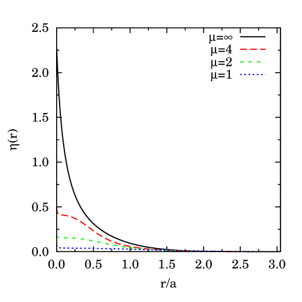
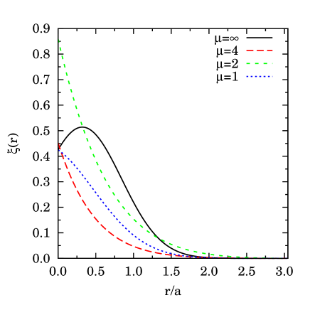
Figure 1: Shows the optimized correlation functions $\eta$ and $\xi$ for $N=54,\zeta=0,$ and $r_{s}=10$ and different values of $\mu$.

VII The radial distribution function (RDF)

The main purpose of the present work is to determine the radial distribution function (RDF) of our fluid model through the DMC calculation.

VII.0.1 Definition of the radial distribution function

The spin-resolved RDF is defined as T. L. Hill (1956); E. Feenberg (1967)

$$g_{\sigma,\sigma^{\prime}}({\bf r},{\bf r}^{{}^{\prime}}) = \frac{\left\langle\sum_{i,j\neq i}\delta_{\sigma,\sigma_{i}}\delta_{\sigma^{\prime},\sigma_{j}}\delta({\bf r}-{\bf r}_{i})\delta({\bf r}^{{}^{\prime}}-{\bf r}_{j})\right\rangle}{n_{\sigma}({\bf r})n_{\sigma^{\prime}}({\bf r}^{{}^{\prime}})}~{},$$ (50)

$$n_{\sigma}({\bf r}) = \left\langle\sum_{i=1}^{N}\delta_{\sigma,\sigma_{i}}\delta({\bf r}-{\bf r}_{i})\right\rangle~{},$$ (51)

where here, and in the following, $\langle\ldots\rangle$ will denote the expectation value respect to the ground-state. Two exact conditions follow immediately from the definition: i. the zero-moment sum rule

$$\sum_{\sigma,\sigma^{\prime}}\int d{\bf r}d{\bf r}^{\prime}\,n_{\sigma}({\bf r})n_{\sigma}({\bf r}^{\prime})[g_{\sigma,\sigma^{\prime}}({\bf r},{\bf r}^{{}^{\prime}})-1]=-N~{},$$ (52)

also known as the charge (monopole) sum rule in the sequence of multipolar sum rules in the framework of charged fluids Ph. A. Martin (1988), ii. $g_{\sigma,\sigma}({\bf r},{\bf r})=0$ due to the Pauli exclusion principle.

For the homogeneous and isotropic fluid $n_{\sigma}({\bf r})=N_{\sigma}/\Omega$ where $N_{\sigma}$ is the number of particles of spin $\sigma$ and $g_{\sigma,\sigma^{\prime}}$ depends only on the distance $r=|{\bf r}-{\bf r}^{{}^{\prime}}|$, so that

$$g_{\sigma,\sigma^{\prime}}(r)=\frac{1}{4\pi r^{2}}\frac{\Omega}{N_{\sigma}N_{\sigma^{\prime}}}\left\langle\sum_{i,j\neq i}\delta_{\sigma,\sigma_{i}}\delta_{\sigma^{\prime},\sigma_{j}}\delta(r-r_{ij})\right\rangle~{}.$$ (53)

The total (spin-summed) radial distribution function will be

$$g(r) = \frac{1}{n^{2}}\sum_{\sigma,\sigma^{\prime}}n_{\sigma}n_{\sigma^{\prime}}g_{\sigma,\sigma^{\prime}}(r)$$ (54)

$$= \left(\frac{1+\zeta}{2}\right)^{2}g_{+,+}(r)+\left(\frac{1-\zeta}{2}\right)^{2}g_{-,-}(r)+\frac{1-\zeta^{2}}{2}g_{+,-}(r)~{}.$$

VII.0.2 From the structure to the thermodynamics

As it is well known the knowledge of the RDF gives access to the thermodynamic properties of the system. The mean potential energy per particle can be directly obtained from $g(r)$ and the bare pair-potential $v_{\mu}(r)$ as follows

$$e_{p}=\sum_{\sigma,\sigma^{\prime}}\frac{n_{\sigma}n_{\sigma^{\prime}}}{2n}\int d{\bf r}\,e^{2}v_{\mu}(r)[g_{\sigma,\sigma^{\prime}}(r)-1]~{},$$ (55)

where we have explicitly taken into account of the background contribution. Suppose that $e_{p}(r_{s})$ is known as a function of the coupling strength $r_{s}$. The virial theorem for a system with Coulomb interactions ($v_{\infty}(r)=1/r$) gives $N(2e_{k}+e_{p})=3P\Omega$ with $P=-d(Ne_{0})/d\Omega$ the pressure and $e_{0}=e_{k}+e_{p}$ the mean total ground-state energy per particle. We then find

$$e_{p}(r_{s})=2e_{0}(r_{s})+r_{s}\frac{de_{0}(r_{s})}{dr_{s}}=\frac{1}{r_{s}}\frac{d}{dr_{s}}[r_{s}^{2}e_{0}(r_{s})]~{},$$ (56)

which integrates to

$$e_{0}(r_{s})=e_{F}+\frac{1}{r_{s}^{2}}\int_{0}^{r_{s}}dr_{s}^{\prime}\,r_{s}^{\prime}e_{p}(r_{s}^{\prime})~{}.$$ (57)

We can rewrite the ground-state energy per particle of the ideal Fermi gas, in reduced units, as

$$e_{F}=\left(\frac{9\pi}{4}\right)^{2/3}\frac{3}{10}\phi_{5}(\zeta)\frac{1}{r_{s}^{2}}~{},$$ (58)

where $\phi_{n}(\zeta)=(1-\zeta)^{n/3}+(1+\zeta)^{n/3}$. And for the exchange potential energy per particle in the Coulomb case

$$e_{p}^{x}=-\left(\frac{2}{3\pi^{5}}\right)^{1/3}\frac{9\pi}{8}\phi_{4}(\zeta)\frac{1}{r_{s}}~{},$$ (59)

which follows from Eq. (55) and Eqs. (63)-(64). The expression for finite $\mu$ can be found in Ref. S. Paziani, S. Moroni, P. Gori-Giorgi, and G. B. Bachelet, 2006 (see their Eqs. (15)-(16)).

VII.0.3 Definition of the static structure factor

If we introduce the microscopic spin dependent number density

$$\rho_{\sigma}({\bf r})=\sum_{i=1}^{N}\delta_{\sigma,\sigma_{i}}\delta({\bf r}-{\bf r}_{i})~{},$$ (60)

and its Fourier transform $\rho_{{\bf k},\sigma}$, then the spin-resolved static structure factors are defined as $S_{\sigma,\sigma^{\prime}}({\bf k})=\langle\rho_{{\bf k},\sigma}\rho_{-{\bf k},\sigma^{\prime}}\rangle/N$, which, for the homogeneous and isotropic fluid, can be rewritten as

$$S_{\sigma,\sigma^{\prime}}(k)=\frac{n_{\sigma}}{n}\delta_{\sigma,\sigma^{\prime}}+\frac{n_{\sigma}n_{\sigma^{\prime}}}{n}\int[g_{\sigma,\sigma^{\prime}}(r)-1]e^{-i{\bf k}\cdot{\bf r}}\,d{\bf r}+\frac{n_{\sigma}n_{\sigma^{\prime}}}{n}(2\pi)^{3}\delta({\bf k})~{},$$ (61)

From now on we will ignore the delta function at ${\bf k}=0$. The total (spin-summed) static structure factor is $S=\sum_{\sigma,\sigma^{\prime}}S_{\sigma,\sigma^{\prime}}$. Due to the charge sum rule (52) we must have $\lim_{k\to 0}S(k)=0$. In Sec. VII.2.2 we will show that the small $k$ behavior of $S(k)$ has to start from the term of order $k^{2}$.

VII.1 Analytic expressions for the non-interacting fermions

Usually $g_{\sigma,\sigma^{\prime}}$ is conventionally divided into the (known) exchange and the (unknown) correlation terms

$$g_{\sigma,\sigma^{\prime}}=g^{x}_{\sigma,\sigma^{\prime}}+g^{c}_{\sigma,\sigma^{\prime}}~{},$$ (62)

where the exchange term corresponds to the uniform system of non-interacting fermions.

VII.1.1 Radial distribution function

We thus have (from the definition of the RDF (50) and using Slater determinants for the wave-function)

$$g^{x}_{+,-}(r) = 1~{},$$ (63)

$$g^{x}_{\sigma,\sigma}(r) = 1-\left[\frac{3j_{1}(k_{F}^{\sigma}r)}{k_{F}^{\sigma}r}\right]^{2}~{},$$ (64)

where $j_{1}(x)=[\sin(x)-x\cos(x)]/x^{2}$ is the spherical Bessel function of the first kind and $(k^{\sigma}_{F})^{3}=6\pi^{2}n_{\sigma}$ is the Fermi wave-number for particles of spin $\sigma$.

VII.1.2 Static structure factor

Again we will have the splitting $S_{\sigma,\sigma^{\prime}}=S_{\sigma,\sigma^{\prime}}^{x}+S_{\sigma,\sigma^{\prime}}^{c}$ into the exchange and the correlation parts. So that for the non-interacting fermions we get

$$S^{x}_{+,-}(k) = 0~{},$$ (65)

$$S^{x}_{\sigma,\sigma}(k) = \frac{n_{\sigma}}{n}-\frac{n_{\sigma}^{2}}{n}\Theta(2k^{\sigma}_{F}-k)\frac{3\pi^{2}}{(k^{\sigma}_{F})^{3}}\left(1-\frac{k}{2k^{\sigma}_{F}}\right)^{2}\left(2+\frac{k}{2k^{\sigma}_{F}}\right)$$ (68)

$$= \frac{n_{\sigma}}{n}\left\{\begin{array}[]{ll}1&k>2k^{\sigma}_{F}\\ \frac{3}{4}\frac{k}{k^{\sigma}_{F}}-\frac{1}{16}\left(\frac{k}{k^{\sigma}_{F}}\right)^{3}&k<2k^{\sigma}_{F}\end{array}\right.~{},$$

where $\Theta(x)$ is the Heaviside step function.

VII.2 RDF sum rules

Both the behavior of the RDF at small $r$ and at large $r$ has to satisfy to general exact relations or sum rules.

VII.2.1 Cusp conditions

When two electrons ($\mu=\infty$) get closer and closer together, the behavior of $g_{\sigma,\sigma^{\prime}}(r)$ is governed by the exact cusp conditions Kimball (1973); *Rajagopal1978; *Hoffmann1992

$$\left.\frac{d}{dr}g_{\sigma,\sigma}(r)\right|_{r\to 0} = 0~{},$$ (69)

$$\left.\frac{d^{3}}{dr^{3}}g_{\sigma,\sigma}(r)\right|_{r\to 0} = \frac{3}{2a_{0}}\left.\frac{d^{2}}{dr^{2}}g_{\sigma,\sigma}(r)\right|_{r\to 0}~{},$$ (70)

$$\left.\frac{d}{dr}g_{+,-}(r)\right|_{r\to 0} = \frac{1}{a_{0}}g_{+,-}(0)~{},$$ (71)

where in the adimensional units $a_{0}\to 1/r_{s}$. For finite $\mu$ we only have the condition $g_{\sigma,\sigma}(0)=0$ due to Pauli exclusion principle.

VII.2.2 The Random Phase Approximation (RPA) and the long range behavior of the RDF

Within the linear density response theory J. P. Hansen and I. R. McDonald (1986); sta one introduces the space-time Fourier transform, $\chi({\bf k},\omega)$, of the linear density response function. Which is related through the fluctuation dissipation theorem, $S({\bf k},\omega)=-(2\hbar/n)\Theta(\omega)\text{Im}\chi({\bf k},\omega)$, to the space-time Fourier transform, $S({\bf k},\omega)$ (dynamic structure factor), of the van Hove correlation function L. van Hove (1954), $\langle\rho({\bf r},t)\rho(\mathbf{0},0)\rangle/n$, where $\rho({\bf r},t)=\exp(iHt/\hbar)\rho({\bf r})\exp(-iHt/\hbar)$.

In the Random Phase Approximation (RPA) we have D. Pines and P. Nozières (1966)

$$\frac{1}{\chi_{RPA}(k,\omega)}=\frac{1}{\chi_{0}(k,\omega)}-e^{2}\tilde{v}_{\mu}(k)~{},$$ (72)

where $\chi_{0}$ is the response function of the non-interacting Fermions (ideal Fermi gas), known as the Lindhard susceptibility J. Lindhard (1954). This corresponds to taking the “proper polarizability” (the response to the Hartree potential) equal to the response of the ideal Fermi gas M. P. Tosi (1999). The RPA static structure factor is then recovered from the fluctuation dissipation theorem as follows

$$S_{RPA}(k)=-\frac{\hbar}{n}\int_{0}^{\infty}\frac{d\omega}{\pi}\,\text{Im}\chi_{RPA}(k,\omega)~{}.$$ (73)

where

$$\text{Im}\chi_{RPA}=\frac{\text{Im}\chi_{0}}{(1-e^{2}\tilde{v}_{\mu}\text{Re}\chi_{0})^{2}+(e^{2}\tilde{v}_{\mu}\text{Im}\chi_{0})^{2}}~{},$$ (74)

The small $k$ behavior of the RPA structure factor is exact D. Pines and P. Nozières (1966). One finds

$$S_{RPA}(k)=\frac{\hbar k^{2}}{2m\omega_{p}}~{},~{}~{}~{}k\ll k_{F}~{},$$ (75)

where $\omega_{p}=\sqrt{4\pi ne^{2}/m}$ is the plasmon frequency G. F. Giuliani and G. Vignale (2005). This is also known as the second-moment sum rule for the exact RDF and can be rewritten as $n\int d{\bf r}\,r^{2}[g(r)-1]=-6(\hbar/2m\omega_{p})$. We can then say that $g(r)-1$ has to decay faster than $r^{-5}$ at large $r$. The fourth-moment (or compressibility) sum rule links the thermodynamic compressibility, $\chi=[nd(n^{2}de_{0}/dn)/dn]^{-1}$, M. P. Tosi (1999) to the fourth-moment of the RDF. For the equivalent classical system it is well known that the correlation functions have to decay faster than any inverse power of the distance A. Alastuey and Ph. A. Martin (1985); Ph. A. Martin (1988); Lighthill (1959) (in accord with the Debye-Hükel theory). We are not aware of the existence of a similar result for the zero temperature quantum case.

VIII Results of the calculation

We considered fourty systems corresponding to $r_{s}=1,2,5,10$, $\mu=\infty,4,2,1,1/2$, $\zeta=0,1$. For each system we calculated the RDF using the histogram estimator in a variational, mixed, and extrapolated measure and a particular HFM measure. Before starting with the simulations we determined the optimal values for the time step $\tau$ and the number of walkers $n_{w}$ for each density.

VIII.1 Extrapolations

For the Coulomb case, $\mu\to\infty$, we made extrapolations in time step $\tau$ and number of walkers $n_{w}$ for each value of $r_{s}$ within our DMC simulations. Given a relative precision $\delta_{e_{0}}=\Delta e_{0}/e_{p}^{x}$, where $e_{0}=\langle E_{L}\rangle_{f}/N$, $\Delta e_{0}$ is the statistical error on $e_{0}$, and $e_{p}^{x}$ is the exchange energy per particle (see Eq. (59)), we set as our target relative precision $\delta_{e_{0}}=10^{-2}\%$.

VIII.1.1 In time step

Our results are summarized in Table 2. As the characteristic dimension of one particle diffusing walk is $\sigma=\sqrt{2\lambda\tau}$ or $\sqrt{2\tau/r_{s}^{2}}$ in adimensional units, this has to remain of the order of the mean nearest neighbor separation $a$ which is chosen to be a constant in our units. Then we expect that at lower $r_{s}$ one needs to choose smaller time steps $\tau$. For this reason we chose different time steps in the simulations of the Table: $\tau=0.5,0.1,0.05$ for $r_{s}=10$, $\tau=0.3,0.1,0.05$ for $r_{s}=5$, $\tau=0.05,0.03,0.005$ for $r_{s}=2$, and $\tau=0.01,0.005,0.001$ for $r_{s}=1$. Note that, at fixed $r_{s}$, the statistical errors increase as the time step diminishes.

Table 2: Extrapolation in time step for $N=66$ unpolarized electrons $(\mu=\infty)$ at a fixed number of $n_{w}=600$ walkers with a trial wave-function of the SJ type. We run the simulation for 3 different time steps and did a linear fit of the $(\tau,e_{0})$ data, $e_{0}=a+b\tau$. The optimal $\tau$ is the largest one compatible with the target precision.

$r_{s}$	$a$	$b$	$\chi^{2}$	optimal $\tau$
10	-0.107456(7)	0.00010(2)	0.9	0.09
5	-0.153352(4)	0.00024(3)	0.1	0.07
2	-0.00416(8)	0.003(2)	4.4	0.01
1	1.14579(7)	0.032(9)	1.1	0.003

VIII.1.2 In the number of walkers

Our results are summarized in Table 3. The fluctuations of the statistical weight of a walker depend on the fluctuations of the local energy, i.e. by the quality of the trial wave-function. The quality of the trial wave-function worsens as $r_{s}$ becomes larger (for the strongly correlated system), and one expects that the necessary number of walkers increases. This is in agreement with the results of the Table. Note that, at fixed $r_{s}$, the statistical errors increase as the number of walkers diminishes.

Table 3: Extrapolation in number of walkers for $N=66$ unpolarized electrons $(\mu=\infty)$ with a time step $\tau=0.1$ for $r_{s}=10,5$, $\tau=0.05$ for $r_{s}=2$, and $\tau=0.01$ for $r_{s}=1$ with a trial wave-function of the SJ type. We run the simulation for 4 different numbers of walkers and did a linear fit of the $(1/n_{w},e_{0})$ data, $e_{0}=a+b/n_{w}$. The optimal $n_{w}$ is the smallest one compatible with the target precision.

$r_{s}$	$a$	$b$	$\chi^{2}$	optimal $n_{w}$
10	-0.107443(3)	0.0032(4)	0.1	354
5	-0.153329(6)	0.0044(7)	0.2	243
2	-0.004036(6)	0.0026(7)	0.2	56
1	1.14609(6)	0.01(1)	1.2	40

VIII.2 Effect of backflow and three-body correlations

In Fig. 2 we show the mixed measure of the RDF calculated in DMC for $N=162,\zeta=0,\mu=\infty,r_{s}=10$ with different kinds of trial wave-functions. Of course in a VMC calculation using the Slater determinant wave-function gives us $g^{x}_{\sigma,\sigma^{\prime}}$, the RDF of the ideal gas (see Eqs. (63)-(64)).

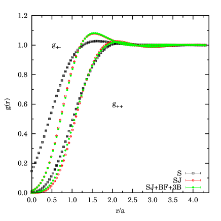
Figure 2: Shows the mixed measure of the RDF calculated in DMC for $N=162,\zeta=0,\mu=\infty,r_{s}=10$ with a S, SJ, SJ+BF+3B trial wave-function.

In Fig. 3 we show the difference between the RDF calculated with the SJ wave-function and the one calculated with the SJ+BF+3B wave-function using the variational, the mixed, and the extrapolated measure.

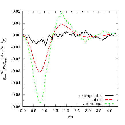
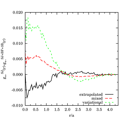
Figure 3: Shows the difference between the RDF calculated with the SJ wave-function and the one calculated with the SJ+BF+3B wave-function using the variational, the mixed, and the extrapolated measure. The results are for $N=162,\zeta=0,\mu=\infty$. On the left the like RDF is used at $r_{s}=10$, on the right the unlike RDF at $r_{s}=1$.

With the extrapolated measure the results from the SJ computation differs by less than $0.005$ from the ones from the SJ+BF+3B. We then decided to perform our subsequent calculations using the SJ trial wave-function.

VIII.3 Size effects

In order to estimate the size effects on the RDF calculation we performed a series of VMC calculation with the SJ wave-function on an unpolarized system with different number of particles. The results (see Fig. 4) show that the size dependence mainly affects the long range behavior of the RDF and the on-top value for the unlike one.

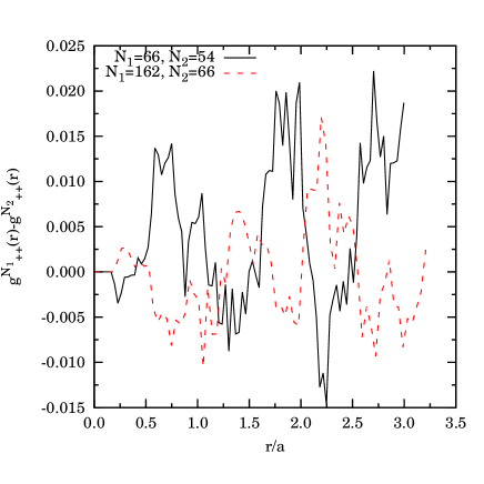
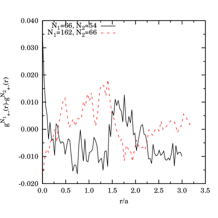
Figure 4: Shows the difference between the RDF of two systems of electrons ($\mu=\infty$) at $r_{s}=10$ and $\zeta=0$ with different sizes $N_{1}$ and $N_{2}$. The RDF are calculated in VMC with the SJ wave-function. On the left the difference of the like RDF is shown and on the right the difference of the unlike RDF is shown.

In the simulation the RDF is defined on $r\in[0,r_{max}]$ with $r_{max}=L/2$ where $L=\Omega^{1/3}=(4\pi N/3)^{1/3}$ is the size of the simulation box. To minimize size effects we chose to perform our RDF calculation with $N=162$ in the unpolarized case and $N=147$ in the polarized case.

VIII.4 The HFM measure

From the definition (53), we can write the RDF as

$$g_{\sigma,\sigma^{\prime}}(r)=\frac{\langle I_{\sigma,\sigma^{\prime}}(r,{\bf R})\rangle}{\Omega n_{\sigma}n_{\sigma^{\prime}}}~{}.$$ (76)

Since the operator $I_{\sigma,\sigma^{\prime}}$ is diagonal in coordinate representation then $I_{\sigma,\sigma^{\prime}}=(I_{\sigma,\sigma^{\prime}})_{L}$. Indicating with $\Omega_{\bf r}$ the solid angle spanned by the ${\bf r}$ vector, we can write

$$I_{\sigma,\sigma^{\prime}}(r,{\bf R})=\sum_{i,j\neq i}\delta_{\sigma,\sigma_{i}}\delta_{\sigma^{\prime},\sigma_{j}}\int\frac{d\Omega_{\bf r}}{4\pi}\delta({\bf r}-{\bf r}_{ij})~{},$$ (77)

which is the usual histogram estimator Allen and Tildesley (1987). Following Toulouse J. Toulouse, R. Assaraf, and C. J. Umrigar (2007) we choose for $Q$ the following expression

$$Q_{\sigma,\sigma^{\prime}}(r,{\bf R})=-\frac{r_{s}^{2}}{8\pi}\sum_{i,j\neq i}\delta_{\sigma,\sigma_{i}}\delta_{\sigma^{\prime},\sigma_{j}}\int\frac{d\Omega_{\bf r}}{4\pi}\frac{1}{|{\bf r}-{\bf r}_{ij}|}~{},$$ (78)

so that (using the identities $\boldsymbol{\nabla}^{2}_{{\bf r}_{ij}}1/|{\bf r}-{\bf r}_{ij}|=-4\pi\delta({\bf r}-{\bf r}_{ij})$ and $\boldsymbol{\nabla}_{{\bf r}_{i}}f({\bf r}_{kj})=\boldsymbol{\nabla}_{{\bf r}_{kj}}f({\bf r}_{kj})[\delta_{ik}-\delta_{ij}]$, for a given function $f$) the first term in Eq. (25) exactly cancels the histogram estimator $I_{\sigma,\sigma^{\prime}}$. Then the HFMv estimator is

$$I_{\sigma,\sigma^{\prime}}^{\text{HFMv}}(r,{\bf R}) = \frac{1}{2\pi}\sum_{i,j\neq i}\delta_{\sigma,\sigma_{i}}\delta_{\sigma^{\prime},\sigma_{j}}{\bf v}_{i}({\bf R})\cdot\int\frac{d\Omega_{\bf r}}{4\pi}\boldsymbol{\nabla}_{{\bf r}_{ij}}\frac{1}{|{\bf r}-{\bf r}_{ij}|}$$ (79)

$$= -\frac{1}{4\pi}\sum_{i,j\neq i}\delta_{\sigma,\sigma_{i}}\delta_{\sigma^{\prime},\sigma_{j}}{\bf v}_{i}({\bf R})\cdot\frac{{\bf r}_{ij}}{r_{ij}^{3}}[1+\text{sgn}(r_{ij}-r)]~{},$$

which goes to zero at large $r$ (see Note shi, ). The correct (taking care of the missing factor of two in Ref. J. Toulouse, R. Assaraf, and C. J. Umrigar, 2007) $\beta$ correction is

$$\Delta I_{\sigma,\sigma^{\prime}}^{\beta}(r,{\bf R}) = -[E_{L}({\bf R})-E_{0}]\frac{r_{s}^{2}}{8\pi}\sum_{i,j\neq i}\delta_{\sigma,\sigma_{i}}\delta_{\sigma^{\prime},\sigma_{j}}\int\frac{d\Omega_{\bf r}}{4\pi}\frac{1}{|{\bf r}-{\bf r}_{ij}|}$$ (80)

$$= -[E_{L}({\bf R})-E_{0}]\frac{r_{s}^{2}}{16\pi}\sum_{i,j\neq i}\delta_{\sigma,\sigma_{i}}\delta_{\sigma^{\prime},\sigma_{j}}\left(\frac{r_{ij}+r-|r_{ij}-r|}{r_{ij}r}\right)~{}.$$

Note that also $\langle\Delta I^{\beta}_{\sigma,\sigma^{\prime}}(r,{\bf R})\rangle$ goes to zero at large $r$. This particular HFM measure needs to be shifted $g_{\sigma,\sigma^{\prime}}(r)=g^{\text{HFM}}_{\sigma,\sigma^{\prime}}(r)+1$. We chose to do the shift as follows: $g_{\sigma,\sigma^{\prime}}(r)=g^{\text{HFM}}_{\sigma,\sigma^{\prime}}(r)+g^{\text{mix}}_{\sigma,\sigma^{\prime}}(L/2)-g^{\text{HFM}}_{\sigma,\sigma^{\prime}}(L/2)$. Nonetheless it is expected to give better results for the on-top value of the RDF where the histogram estimator of Eq. (53), after the necessary discretization of the Dirac delta function, leads, in the measure, to a statistical average divided by zero. Moreover it does not suffer from any discretization error and can be calculated for any value of $r$.

In Fig. 5 we show a comparison for the RDF of the $N=162,\zeta=0,\mu=\infty,r_{s}=10$ system, calculated in DMC SJ with various kinds of measures. The length of the run was always the same 50 blocks of 500 steps each. From the figure one can see that with our choice of the $\beta$ correction the HFM measure has the correct average value (coinciding with the usual histogram estimator). From the figure it is also evident that the HFM measure is much less efficient than the other measures (clearly with a sufficient number of blocks the statistical error on the HFM measure can be made small at will).

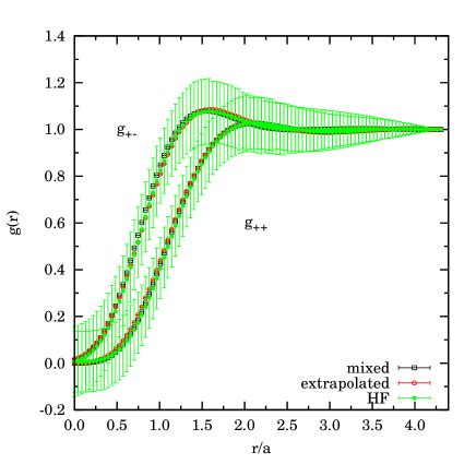
Figure 5: Shows the RDF of the $N=162,\zeta=0,\mu=\infty,r_{s}=10$ system, calculated in DMC SJ with various kinds of measures: mixed histogram (mixed), extrapolated histogram (extrapolated), and HFM (HFM) with the choice of Eq. (78).

This inefficiency is entirely due to the ZB correction (essential in the DMC calculation). From its definition (see Eq. (80)) one can see that it is the small difference of two large terms involving the (extensive) total energy . So the statistical error on the HFM measure is completely dominated by that of the $\beta$ part, the $\alpha$ part having statistical errors comparable with the ones of the usual histogram estimator, as shown in the left panel of Fig. 6.

VIII.5 Choice of the Jastrow

We noticed that at small $r_{s},\mu,$ and $r$ the variational measure for the unlike RDF, with the chosen Jastrow ${\cal J}_{1}$ of Eq. (38), deviates strongly from the mixed one. This is no longer so with the modified Jastrow ${\cal J}_{2}$ of Eq. (43) which at small $\mu$ gives also better variational energies (but not for $\mu\to\infty$ where ${\cal J}_{1}$ is better. Note that the Jastrow factor does not change the nodes of the wave-function so the energies calculated from the diffusion with ${\cal J}_{1}$ or ${\cal J}_{2}$ coincide). The extrapolated measures do not change appreciably in the two cases apart from near $r=0$. In Fig. 6 we show the difference for the two calculations with ${\cal J}_{1}$ and ${\cal J}_{2}$ for the $\zeta=0,r_{s}=1,\mu=1$ model. From the inset in the left panel we can see that among the two extrapolated measures there is a difference of the order of 0.005.

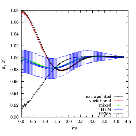
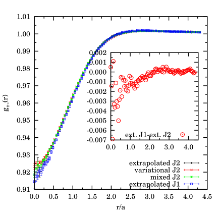
Figure 6: Unlike RDF for the unpolarized fluid of Paziani S. Paziani, S. Moroni, P. Gori-Giorgi, and G. B. Bachelet (2006) at $r_{s}=1$ and $\mu=1$ with $N=162$. On the left the calculation with the Jastrow ${\cal J}_{1}$ of Eq. (38) with various measures: variational histogram (variational) and variational HFMv (HFMv) using the estimator of Eq. (79), mixed histogram (mixed) and HFM (HFM), and extrapolated histogram (extrapolated). On the right the calculation with the Jastrow ${\cal J}_{2}$ of Eq. (43) with the histogram variational (variational), mixed (mixed), and extrapolated (extrapolated) measures. In the inset is shown the difference between the histogram extrapolated measure of the calculation with ${\cal J}_{1}$ and the histogram extrapolated measure of the calculation with ${\cal J}_{2}$. $10^{5}$ Monte Carlo steps were used in the simulations.

Our results with the two Jastrow factors show that ${\cal J}_{1}$ is better than ${\cal J}_{2}$ for the near-Jellium systems ($\mu$ large) while ${\cal J}_{2}$ is better than ${\cal J}_{1}$ for the near-ideal systems ($\mu$ small).

VIII.6 The histogram estimator

In Fig. 7 we show the DMC results for the histogram extrapolated measure of the RDF of our fluid model at $\zeta=0$. The time step, $\tau$, and number of walkers, $n_{w}$, were chosen according to the indications given in subsection VIII.1. Fig. 8 is for the $\zeta=1$ case.

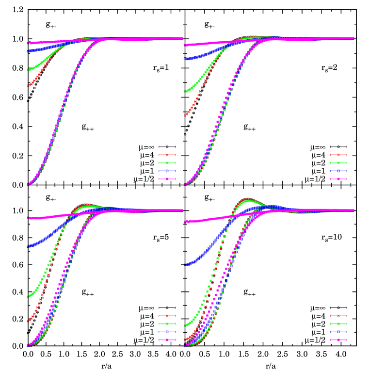
Figure 7: Shows the histogram extrapolated measure for the RDF of a system of 162 unpolarized ($\zeta=0$) particles calculated using the SJ trial wave-function. The VMC calculation was made of $10^{6}$ steps while the DMC by $10^{5}$. The trial wave-function used was of the SJ type with the Jastrow ${\cal J}_{1}$ of Eq. (38).

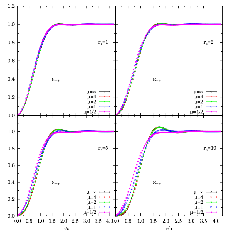
Figure 8: Shows the histogram extrapolated measure for the RDF of a system of 147 fully polarized ($\zeta=1$) particles calculated using the SJ trial wave-function. The VMC calculation was made of $10^{6}$ steps while the DMC by $10^{5}$. The trial wave-function used was of the SJ type with the Jastrow ${\cal J}_{1}$ of Eq. (38).

In Table 4 we show the on-top values for the unlike RDF, $g_{+-}(0)$, of the unpolarized system, calculated with the histogram variational, the histogram mixed, the histogram extrapolated measure, the HFM measure, and the HFM extrapolated measure (of Eq. (24)).

Table 4: Contact values for the unlike RDF of the unpolarized fluid of Paziani S. Paziani, S. Moroni, P. Gori-Giorgi, and G. B. Bachelet (2006), at various $r_{s}$ and $\mu$, from the histogram variational (variational), mixed (mixed), and extrapolated (extrapolated) measures, and the HFM (HFM) and HFM extrapolated (HFM-ext) measures. The trial wave-function used was of the SJ type with the Jastrow ${\cal J}_{1}$ of Eq. (38). The last column gives the error $\sigma_{\text{av}}=\sqrt{\sigma^{2}{\cal K}/{\cal N}}$ ($\sigma^{2}$ is the variance, ${\cal K}$ the correlation time of the random walk, and ${\cal N}$ the number of Monte Carlo steps) on the HFM measure. $162$ particles were used with $10^{5}\times n_{w}$ Monte Carlo steps.

$r_{s}$	$\mu$	variational	mixed	extrapolated	HFM	HFM-ext	$\sigma_{av}$ on HFM
10	1/2	1.085(8)	1.000(4)	0.91(1)	1.0006	0.9222	0.03
10	1	0.706(6)	0.644(3)	0.582(8)	0.6474	0.5949	0.03
10	2	0.219(4)	0.182(1)	0.146(4)	0.1798	0.1450	0.06
10	4	0.053(2)	0.0506(8)	0.048(2)	0.0460	0.0394	0.07
10	$\infty$	0.0074(6)	0.0096(3)	0.0118(8)	0.0045	0.0029	0.09
5	1/2	1.129(8)	1.034(3)	0.94(1)	1.0277	0.9381	0.03
5	1	0.850(7)	0.796(3)	0.743(9)	0.7912	0.7325	0.02
5	2	0.448(5)	0.405(2)	0.362(6)	0.4022	0.3565	0.02
5	4	0.214(3)	0.199(1)	0.184(4)	0.1960	0.1782	0.03
5	$\infty$	0.080(2)	0.0799(8)	0.080(2)	0.0625	0.0557	0.03
2	1/2	1.158(8)	1.0618(4)	0.97(1)	1.0545	0.9484	0.04
2	1	1.003(8)	0.927(3)	0.852(9)	0.9270	0.8561	0.03
2	2	0.754(7)	0.697(3)	0.639(9)	0.6919	0.6299	0.02
2	4	0.549(6)	0.511(2)	0.473(7)	0.5127	0.4687	0.02
2	$\infty$	0.376(4)	0.349(2)	0.323(5)	0.3236	0.3030	0.02
1	1/2	1.171(8)	1.077(3)	0.98(1)	1.0705	0.9683	0.02
1	1	1.077(8)	0.994(3)	0.91(1)	0.9938	0.9070	0.02
1	2	0.924(8)	0.855(3)	0.787(9)	0.8640	0.8053	0.02
1	4	0.784(7)	0.730(2)	0.676(8)	0.7295	0.6628	0.01
1	$\infty$	0.645(6)	0.602(2)	0.560(7)	0.5771	0.5263	0.01

IX Conclusions

We studied through Variational and Diffusion Monte Carlo techniques the fluid of spin one-half particles interacting with the bare pair-potential $v_{\mu}(r)=\text{erf}(\mu r)/r$ and immersed in a uniform counteracting background. When $\mu\to\infty$ the system reduces to the Jellium model whereas when $\mu\to 0$ it reduces to the ideal Fermi gas. We performed a detailed analysis of the spin-resolved Radial Distribution Function for this system as a function of the density parameter $r_{s}=1,2,5,10$ and the penetrability parameter $\mu=1/2,1,2,4,\infty$ at two values of the polarization, $\zeta=0,1$.

Initially we carefully fine tuned our DMC calculation determining the optimal values for the time step $\tau$ and the number of walkers $n_{w}$ for each value of the density parameter $r_{s}$. Increasing the system size $N$ the RDF extends its range $[0,r_{max}]$ at larger $r_{max}$. We estimated that for $N\geq 66$ the size dependence of the RDF is lower than 2%. As a compromise between computational cost and reduction of the size effects, the largest uncontrolled source of uncertainty on our RDF measurements, we chose to perform the RDF calculation with $N=162$ in the unpolarized case and $N=147$ in the polarized case.

We calculated the RDF using two different routes: through the usual histogram estimator and through a particular HFM measure. As expected, in the VMC calculations the HFMv estimator gives better results for the on-top value of the RDF. In the DMC calculation the inclusion of the $\beta$ correction (which must be omitted in the VMC calculation) is indispensable. Moreover the ZV estimator is zero for $r>r_{max}$ so it has to be shifted by $+1$. From our variational and fixed nodes diffusion Monte Carlo experiments turns out that although in the variational measure the average of the histogram estimator agrees with the average of the HFMv estimator within the square root of the variance of the average $\sigma_{\text{av}}=\sqrt{\sigma^{2}{\cal K}/{\cal N}}$, where $\sigma^{2}$ is the variance, ${\cal K}$ the correlation time of the random walk, and ${\cal N}$ the number of Monte Carlo steps, and the two $\sigma_{\text{av}}$ are comparable, in the diffusion experiment, where one has to add the $\beta$ correction not to bias the average, the Hellmann and Feynman measure has an average in agreement with the one of the histogram estimator but the $\sigma_{\text{av}}$ increases. This is to be expected from the extensive nature of the $\beta$ correction in which the energy appears. Of course the averages from the extrapolated Hellmann and Feynman measure and the extrapolated measure for the histogram estimator also agree.

In the simulation, for the Coulomb case, $\mu\to\infty$, we made extrapolations in time step and number of walkers for each value of $r_{s}$. Given a relative precision $\delta_{e_{0}}=\Delta e_{0}/e_{p}^{x}$, where $e_{0}=\langle E_{L}\rangle_{f}/N$, $\Delta e_{0}$ is the statistical error on $e_{0}$, and $e_{p}^{x}$ is the exchange energy, we set as our target relative precision $\delta_{e_{0}}=10^{-2}\%$. The extrapolated values of the time step and number of walkers was then used for all other values of $\mu$. We chose the trial wave function of the Bijl-Dingle-Jastrow Bij form as a product of Slater determinats and a Jastrow factor. The pseudo potential was chosen as in Ref. D. M. Ceperley (2004), ${\cal J}_{2}$, which is expected to give better results for Jellium. Comparison with the simulation of the unpolarized fluid at $r_{s}=1$ and $\mu=1$ with the pseudo potential of Ref. D. Ceperley (1978), ${\cal J}_{1}$, for which the trial wave function becomes the exact ground state wave function in the $\mu\to 0$ limit, show that the two extrapolated measures of the unlike histogram estimator differ one from the other by less than $7\times 10^{-3}$, the largest difference being at contact (see Fig. 1). The use of more sophisticated trial wave functions, taking into account the effect of backflow and three-body correlations, is found to affect the measure by even less in the range of densities considered. For the same reason we discarded the use of the twist-averaged boundary conditions C. Lin, F. H. Zong, and D. M. Ceperley (2001) and only worked with periodic boundary conditions. In Table 4 we compare the contact values of the unlike RDF of the unpolarized fluid at various $r_{s}$ and $\mu$ from the measures of the histogram estimator and the HFM measures. We see that there is disagreement between the measure from the histogram estimator and the HFM measure only in the Coulomb $\mu\to\infty$ case at $r_{s}=1,2$.

Our results complement the ones of Paziani et al. S. Paziani, S. Moroni, P. Gori-Giorgi, and G. B. Bachelet (2006) which only reported a limited number of RDF data. We plan, in the future, to complete the calculation at intermediate polarizations, $0<\zeta<1$, complementing the work of Ortiz and Ballone G. Ortiz and P. Ballone (1994), and Ceperley and coworkers Y. Kwon, D. M. Ceperley, and R. M. Martin (1998).

We believe it is still an open problem the one of determining the relationship between the choice of the auxiliary function, the bias it introduces in the Hellmann and Feynman measure, and the variance of this measure.

Appendix A Jastrow, backflow, and three-body

In terms of the stochastic process governed by $f({\bf R},t)$ one can write, using Kac theorem M. Kac (1959); Kac (1951)

$$\int d{\bf R}\,f({\bf R},\tau)=\left\langle\exp\left[-\int_{0}^{\tau}dt\,E_{L}({\bf R}^{t})\right]\right\rangle_{\text{DRW}}~{},$$ (81)

where $\langle\ldots\rangle_{\text{DRW}}$ means averaging with respect to the diffusing and drifting random walk. Choosing a complete set of orthonormal wave-functions $\Psi_{i}$ we can write for the true time dependent many-body wave-function

$$\phi({\bf R},\tau) = \sum_{i}\Psi_{i}({\bf R})\int d{\bf R}^{\prime}\Psi_{i}({\bf R}^{\prime})\phi({\bf R}^{\prime},\tau)\approx\Psi({\bf R})\int d{\bf R}\,f({\bf R},\tau)$$ (82)

$$= \Psi({\bf R})\left\langle\exp\left[-\int_{0}^{\tau}dt\,E_{L}({\bf R}^{t})\right]\right\rangle_{\text{DRW}}~{},$$

where $\Psi$ is the wave-function, of the set, of maximum overlap with the true ground-state, the trial wave-function. Assuming that at time zero we are already close to the stationary solution, for sufficiently small $\tau$ we can approximate

$$\left\langle\exp\left[-\int_{0}^{\tau}dt\,E_{L}({\bf R}^{t})\right]\right\rangle_{\text{DRW}}\approx e^{-\tau E_{L}({\bf R}^{\tau})}~{}.$$ (83)

By antisymmetrising we get the Fermion wave-function

$$\phi_{F}({\bf R},\tau)\approx{\cal A}\left[e^{-\tau E_{L}({\bf R})}\Psi({\bf R})\right]~{},$$ (84)

where given a function $f({\bf R})$ we define the operator (a symmetry of the Hamiltonian)

$${\cal A}[f({\bf R})]=\frac{1}{N_{P}}\sum_{P}(-1)^{P}f(P{\bf R})~{},$$ (85)

here $N_{P}=N_{+}!N_{-}!$ is the total number of allowed permutations $P$.

This is called the local energy method to improve a trial wave-function. Suppose we start from a simple unsymmetrical product of single particle plane waves of $N_{+}$ spin-up particles with $k<k_{F}^{+}$ occupied and $N_{-}$ spin-up particles with $k<k_{F}^{-}$ occupied, for the zeroth order trial wave-function. Equation (84) will give us a first order wave-function of the Slater-Jastrow type (see equation (27)). If we start from an unsymmetrical Hartree-Jastrow trial wave-function the local energy with the Jastrow factor has the form

$$E_{L}=V-\lambda\sum_{i}\left[-k_{i}^{2}-2i{\bf k}_{i}\cdot\boldsymbol{\nabla}_{i}\sum_{j<k}u(r_{jk})-\boldsymbol{\nabla}_{i}^{2}\sum_{j<k}u(r_{jk})+\left|\boldsymbol{\nabla}_{i}\sum_{j<k}u(r_{jk})\right|^{2}\right]~{},$$ (86)

where $V=V({\bf R})$ is the total potential energy and $r_{ij}=|{\bf r}_{ij}|=|{\bf r}_{i}-{\bf r}_{j}|$. Then the antisymmetrized second order wave-function has the form in Eq. (44), which includes backflow (see the third term), which is the correction inside the determinant and which affects the nodes, and three-body boson-like correlations (see last term) which do not affect the nodes.