Excitation spectra from angular momentum projection of Hartree-Fock states and the configuration-interaction shell-model

Abstract

We make numerical comparison of spectra from angular-momentum projection on Hartree-Fock states with spectra from configuration-interaction nuclear shell-model calculations, all carried out in the same model spaces (in this case the $sd$, lower $pf$, and $p$-$sd_{5/2}$ shells) and using the same input Hamiltonians. We find, unsurprisingly, that the low-lying excitation spectra for rotational nuclides are well reproduced, but the spectra for vibrational nuclides, and more generally the complex specta for odd-A and odd-odd nuclides are less well reproduced in detail.

I Introduction

In Hartree-Fock (HF) calculations, one approximates the ground state by a single Slater determinant (antisymmeterized product of single-particle wavefunctions) and minimizes the energy, reducing the many-body problem to an effective one-body problem ring . The Hartree-Fock solution can break exact symmetries, such as rotational invariance, and indeed is often more effective if it breaks exact symmetries. Restoring broken symmetries adds correlations that further lower the energy and is a useful approach for many problems.

In this paper we project states of good angular momentum from a Hartree-Fock state, and compare the resulting ground state energies and, especially, excitation spectra to exact results from equivalent full configuration-interaction diagonalization in a shell-model basis. Such comparisons help us to understand the accuracy and limitations of the projected Hartree-Fock approximation (PHF), as well as potentially providing a useful shortcut to nuclear structure.

PHF is not new PY57 and can be found in a number of variants. Most of these are inspired by the Nilsson model Ni55 ; La80 and the Elliott SU(3) model El58 , and they can be classified by their use of (a) quasiparticle single-particle states (b) mixing of particle-hole states and (c) schematic or realistic interactions. For example, the projected shell model (PSM) uses quasiparticle single-particle states but no mixing of particle-hole states and schematic interactions PSM ; the MONSTER and VAMPIR codes use quasiparticle single-particle states, and mixing of particle-hole states, and realistic interactions VAMPIRetc ; and the projected configuration-interaction (PCI) eschews quasiparticles states but uses realistic interactions and mixes higher-order particle-hole states PCI . This list is not exhaustive.

What is new in this paper is the comparison of exact numerical solutions against a relatively simple state, with a focus on the quality of the excitation spectra. In this case the “exact” solution is from a full configuration-interaction (CI) calculation, using semi-realistic interactions diagonalized in a truncated but nontrivial shell-model basis, against a single Hartree-Fock state with angular momentum projection. Hence we eschew quasiparticle states and particle-hole states, but we use a realistic interaction and we allow arbitrary deformation.

This paper is similar in philosophy to previous work comparing the random phase approximation (RPA) against CI calculations in a CI basis SHERPA ; SJ02 , testing how good is a specific approximation against a numerically exact result; in the former work the approximation was RPA, while here it is PHF. Another similar set of papers are those on PCI PCI , which compare results directly to CI diagonalization. An important difference with much previous work, however, is that in addition to studying the trends of the ground state energies, we consider in detail the excitation spectra.

We find that rotational spectra, and spectra that are from simple particle-rotor coupling, are well reproduced, with a small rms error. Other excitation spectra, such as vibrational spectra or complex spectra from odd-$A$ and odd-odd nuclides, have larger rms errors. This is unsurprising, but it is useful to verify in detail as we have done.

In the next two sections we outline the numerical exact (CI) and approximate (HF and PHF) calculations, which we then compare for a variety of nuclides in Section V

II The shell-model basis and configuration-interaction calculations

We begin by outlining the shell-model basis in which we work and the fundamentals of configuration-interaction calculations BG77 ; BW88 ; SMreview05 .

We work entirely in occupation or configuration space. This means that we start with some finite set of orthonormal single-particle states, $\{\phi_{a}(\vec{r})\}$. Each of these states have good angular momentum and parity and are labeled by orbital $l$, total $j$, and $z$-component $j_{z}$; implicitly they have good spin $s$, which here is 1/2 although other values are allowed by our code. We also have two species of particles, here protons and neutrons, each with fixed numbers.

Using second quantization we have fermion creation and annihiliation operators $\hat{\phi}_{a}^{\dagger},\hat{\phi}_{a}$ that create or remove a particle from the states $\phi_{a}(\vec{r})$. The uncoupled Hamiltonian is then

$$\hat{H}=\sum_{ab}T_{ab}\hat{\phi}^{\dagger}_{a}\hat{\phi}_{b}+\frac{1}{4}\sum_{abcd}V_{ab,cd}\hat{\phi}^{\dagger}_{a}\hat{\phi}^{\dagger}_{b}\hat{\phi}_{d}\hat{\phi}_{c}$$ (1)

The one-body and two-body matrix elements, $T_{ab}$ and $V_{ab,cd}$ respectively, are appropriate integrals over the Hamiltonian and the single-particle states BG77 . Because the Hamiltonian is an angular momentum scalar, we store the matrix elements in coupled form. Given the single-particle space, the matrix elements are generated externally to all our codes and read in from a file. Any radial form of the single-particle states and any form of the interaction, including non-local interactions, are allowed and make no pratical difference to our many-body codes. Because we work in second quantization, the two-body matrix elements are automatically antisymmeteric and we do not separate direct from exchange terms.

For configuration-interaction (CI) calculations we use the BIGSTICK code BIGSTICK . BIGSTICK creates a many-body basis of Slater determinants $\{|\alpha\rangle\}$, constructed from the single-particle basis:

$$|\alpha\rangle=\prod_{a=1}^{N_{p}}\hat{\phi}^{\dagger}_{a}|0\rangle,$$ (2)

where $N_{p}$ is the number of particles (occupied states). We fix the total $M=J_{z}$ of the many-body basis states, (this is trivial as each single-particle state has good $j_{z}$ as well) and is thus called an $M$-scheme code; because the Hamiltonian is an angular momentum scalar, the final eigenstates thus will automatically have good total angular momentum $J$ (and isospin $T$, although we have the capability to break isospin; $T_{z}=(Z-N)/2$ is fixed). Within the fixed single-particle space and fixed $J_{z},T_{z}$ we allow all possible configurations.

Given the basis, BIGSTICK then computes the many-body Hamiltonian matrix elements $\langle\alpha|\hat{H}|\beta\rangle$ and finds the low-lying eigenstates, including the ground state, using the Lanczos algorithm Lanczos ; SMreview05 . With the single-particle space and Hamiltonian matrix elements fixed, the resulting eigenenergies for the full-space CI calculation are numerically exact. BIGSTICK can handle CI $M$-scheme model spaces on a desktop computer up to dimension roughly 2-400 million.

III Hartree-Fock approximation

The Hartree-Fock approximation (HF) is a variational method using a single Slater determinant ring . One applies a unitary transformation among the single-particle states:

$$\hat{c}_{i}=\sum_{a=1}^{N_{s}}U_{ai}\hat{\phi}_{a},$$ (3)

where $N_{s}$ is the number of single-particle basis states (hence the number of particles $N_{p}<N_{s}$) and creates the trial Slater determinant

$$|\Psi_{T}\rangle=\prod_{i=1}^{N_{p}}\hat{c}^{\dagger}_{i}|0\rangle.$$ (4)

Then one finds a Slater determinant that minimizes the energy, that is, that minimizes

$$E=\frac{\langle\Psi_{T}|\hat{H}|\Psi_{T}\rangle}{\langle\Psi_{T}|\Psi_{T}\rangle}$$ (5)

Because our input matrix elements are antisymmeterized, we fully include both direct and exchange terms. Working in occupation space the exchange term causes us no difficulty (or, to put it another way, any difficulty is off-shored into calculation of the antisymmeterized integrals).

Many Hartree-Fock calculations enforce good angular momentum, for closed-shell systems or closed-shell plus or minus one particle. Our HF code (the SHERPA code SHERPA ) allows the Slater determinant to break rotational invariance, even for closed-shell systems; such Slater determinants are ‘deformed.’ Experience in nuclear physics suggest this to be a fruitful path. Our only constraint is that we assume the transformation (3) to be real.

In order to minimize, we use the standard Hartree-Fock equations, which consist of iteratively solving

$$\mathbf{h}\vec{u}_{i}=\epsilon_{i}\vec{u}_{i},$$ (6)

where the Hartree-Fock effective one-body Hamiltonian is

$$h_{ab}=T_{ab}+\sum_{cd}V_{ac,bd}\rho_{dc}$$ (7)

and

$$\rho_{dc}=\sum_{i=1}^{N}U_{ic}U_{id}$$ (8)

We have separate Slater determinants for proton and neutrons; the generalization is straight forward. More details are found in Appendix A.

IV Projection of angular momentum and parity

In order to project out angular momentum, we introduce the standard projection operator La80 ; ring

$$\hat{P}^{J}_{MM^{\prime}}=\int d\Omega{\cal D}^{(J)*}_{MM^{\prime}}(\Omega)\hat{R}(\Omega),$$ (9)

where $\Omega=\alpha,\beta,\gamma$ and $d\Omega=d\alpha\sin\beta d\beta d\gamma$, ${\cal D}^{(J)*}_{MM^{\prime}}$ is the Wigner $D$-matrix Edmonds , and $\hat{R}(\Omega)$ is the rotation operator. The rotation operator acts on a Slater determinant $U$ whose columns are single-particle states with good $j,m$; therefore the matrix elements of $\hat{R}$ are given by the Wigner $D$-matrix:

$$\langle j^{\prime}m^{\prime}|\hat{R}|jm\rangle=\delta_{j^{\prime}j}D^{j}_{m^{\prime}m}(\alpha\beta\gamma).$$ (10)

It is useful to note that the $j,m,m^{\prime}$ for the rotational matrix $\hat{R}$ are those of the single-particle space, while the $J,M,M^{\prime}$ for the projection operator (9) are those of the many-body space.

We now introduce the Hamiltonian and “norm” matrix elements,

$$h^{J}_{M,M^{\prime}}\equiv\langle\Psi|\hat{H}\hat{P}^{J}_{M,M^{\prime}}|\Psi\rangle,\,\,\,n^{J}_{M,M^{\prime}}\equiv\langle\Psi|\hat{P}^{J}_{M,M^{\prime}}|\Psi\rangle$$ (11)

These are both Hermitian.

Then we solve the generalized eigenvalue equation

$$\sum_{M^{\prime}}h^{J}_{M,M^{\prime}}g^{J}_{M^{\prime}}=E^{J}\sum_{M^{\prime}}n^{J}_{M,M^{\prime}}g^{J}_{M^{\prime}}.$$ (12)

where we allow $g_{M}$ to be complex. Although the deformed Hartree-Fock state will have an orientation, the final result will be independent of orientation; we confirmed this by arbitrarily rotating our HF state.

PHF will only generate a limited number of states. For a given $J$, the maximum number is $(2J+1)$, although fewer can be found if the norm matrix $n$ has zero, or very small, eigenvalues. This can happen, for example, if the HF state has axial symmetry. Therefore there will be states missing from the CI spectrum, such as low-lying excited $J=0$ states.

V Results

In this section we apply our calculations to a number of nuclides in the $sd$ and $pf$ shells as well as a limited $p$-$sd$ space where we allow for parity-projection as well. We ask a number of questions:

$\bullet$ Because PHF is a variational theory, the PHF ground state energy will be above the exact ground state energy. We ask: what is the systematics of that displacement? For example, if the displacement were nearly constant, we could use PHF to reliably estimate the true ground state energy.

$\bullet$ In a similar fashion we ask, how well does PHF yield the excitation spectrum?

$\bullet$ For odd-$A$ and odd-odd nuclei, how often does PHF yield the correct $J^{\pi}$ assignment for the ground state?

$\bullet$ For multi-shell calculations, how well does parity+angular-momentum projection yield the splitting of positive and negative parity spectra?

Many previous studies have focused on the ground state energy. By contrast, we focus on the excitation spectrum, as well as systematics of the ground state energy.

We work with several model spaces and interactions. All model spaces assume some inert core and valence particles; the single-particle states can be thought of as spherical harmonic oscillator wavefunctions, but that has no impact on our calculations. The interactions we use are all ‘realistic,’ based on effective interactions derived from scattering data but with individual matrix elements adjusted to fit many-body data (see BG77 ; br06 for details of methodology). The three model spaces we work in and their interactions are:

$\bullet$ sd, or the 1$s_{1/2}$-$0d_{3/2}$-$0d_{5/2}$ valence space, assuming an inert ¹⁶O core; the interaction is the universal $sd$-interaction ‘B,’ or USDB br06 ;

$\bullet$ pf, or the $1p_{1/2}$-$1p_{3/2}$-$0f_{5/2}$-$0f_{7/2}$ valence space, assuming an inert ⁴⁰Ca core; the interaction is the monopole-modified Kuo-Brown G-matrix interaction version 3G, or KB3G KB3G ;

$\bullet$ and finally the psd, or $0p_{3/2}$-$0p_{1/2}$-$0d_{5/2}$- $1s_{1/2}$ valence space, assuming an inert ⁴He core; the interation is a hybrid of Cohen-Kurath (CK) matrix elements in the $0p$ shellCK65 , the older universal $sd$ interaction of Wildenthal Wildenthal in the $0d_{5/2}$-$1s_{1/2}$ space, and the Millener-Kurath (MK) $p$-$sd$ cross-shell matrix elementsMK75 . We leave out the $0d_{3/2}$ orbit is to make full shell-model calculations tractable. Within the $p$ and $sd$ spaces we use the original spacing of the single-particle energies for the CK and Wildenthal interactions, respectively, but then shift the $sd$ single-particle energies up or down relative to the $p$-shell single particle energies to we get the first $3^{-}$ state at approximately $6.1$ MeV above the ground state. The rest of the spectrum, in particular the first excited $0^{+}$ state, is not very good, but the idea is to have a non-trivial model, not exact reproduction of the spectrum. This model space and interaction allows us to consider model nuclei with both parities and to investigate parity-mixing in the HF state.

To illustrate our results, we begin with ²⁴Mg in the $sd$ shell. Fig. 1 compares the exact CI spectrum on the right against the PHF spectrum on the left. The PHF g.s. is 1.78 MeV above the CI g.s., while on average each states in the PHF spectrum is shifted by 1.68 MeV. For comparison, the correlation energy, here defined as the difference between the unprojected HF energy and the CI g.s. energy, is 6.62 MeV, so that restoring good $J$ by projection accounts for $73\%$ of the correlation energy.

Fig. 2 is the same as Fig. 1 but with the PHF spectrum shifted down so the g.s. energies coincide. The agreement between the excitation spectra is very good, with an rms error of 0.10 MeV.

Other nuclides shall qualitatively similar results, albeit with varying degrees of accuracy. In general the PHF excitation spectra of even-even nuclides was of much higher accuracy than for odd-odd and odd-$A$ nuclides, which is not too surprising as one might expect a deformed HF state to approximate a rotational band.

For example, consider the odd-odd nuclide ³⁰Al in the $sd$ shell, as shown in Fig. 3. The PHF g.s. is 6.40 MeV above the CI g.s., and PHF only accounts for $25\%$ of the correlation energy. When the PHF g.s. is shifted down to the match the CI g.s., Fig. 4, the rms error in the excitation spectrum is 0.66 MeV and many of the states are out of order–in particular the first excited $1^{+}$ state.

This continues in the $pf$ shell. In Fig. 5 we show ⁵²Ti, which has a strong vibrational rather than rotational spectrum. Here the PHF g.s. energy is 3.16 MeV above the CI g.s., account for only $42\%$ of the correlation energy, and even when the PHF spectrum is shifted down in Fig. 6, it is clearly compressed relative to the exact CI, with an rms error of 0.53 MeV.

By contrast, the spectrum of ⁴⁹Cr, which can be thought of as a particle-rotor coupled nucleus, is good. As shown in Fig.  7, the PHF g.s. is 2.63 MeV above the CI g.s., and PHF accounts for only $35\%$ of the correlation energy; but when the PHF spectrum is shifted down, as in Fig. 8, the rms error is only 0.01 MeV.

We also worked in a cross-shell system, the $p$-$sd_{5/2}$ space. Keep in mind we artificially reduced the separation between the $p$ and $sd_{5/2}$ shells in order to provoke a parity-mixed HF state.

The vibrational spectrum the positive parity states of ¹⁸C is only modestly reproduced by PHF, as illustrated in Fig. 9 and 10. The PHF g.s. is 3.84 MeV above the CI g.s., accounting for only $44\%$ of the correlation energy, and when the PHF spectrum is shifted to match the g.s. energies, the rms error is 0.22 MeV, with the $4^{+}$ state in the wrong place.

Somewhat better are the positive parity states of ²²F, in Figs. 11 and 12. The PHF state is 1.41 MeV above the CI g.s., but that only accounts for barely $15\%$ of the correlation energy. On the other hand, when the g.s. energies are matched, the error in the excitation is only 0.08 MeV, although some of the states are in the wrong order.

Tables I and II summarize our results. In particular, Table I summarizes for specific cases the standard deviation (rms error) of the PHF excitation spectra relative to the CI excitation spectra, once the ground state energies are matched. Table II summarizes all our calculations; the rightmost column gives how often the correct g.s. $J^{\pi}$ arises out of the PHF. Even-even nuclides almost always get the correct $J=0$ ground state (but for our mixed-shell calculations, occasionally the wrong parity–but keep in mind we artificially reduced the splitting between the shells to force a mixed-parity HF state), but odd-$A$ got the correct g.s. assignment only a little over half the time, and odd-odd nuclei less than half the time.

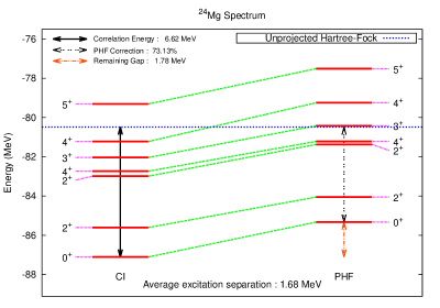
Figure 1: Comparison of exact CI and PHF spectra of ²⁴Mg in the $sd$ model space with the USDB interaction.

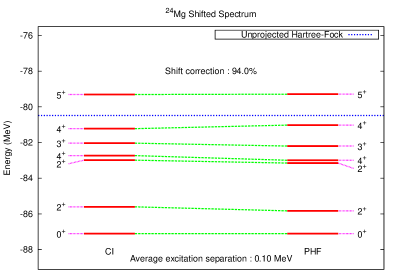
Figure 2: Comparison of exact CI and PHF spectra of ²⁴Mg in the $sd$ model space with the USDB interaction, but with the PHF spectrum shifted downwards so the g.s. energies coincide.

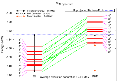
Figure 3: Comparison of exact CI and PHF spectra of ³⁰Al in the $sd$ model space with the USDB interaction.

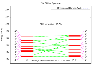
Figure 4: Comparison of exact CI and PHF spectra of ³⁰Al in the $sd$ model space with the USDB interaction, but with the PHF spectrum shifted downwards so the g.s. energies coincide.

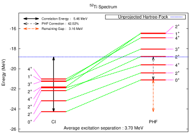
Figure 5: Comparison of exact CI and PHF spectra of ⁵²Ti in the $pf$ model space with the KB3G interaction.

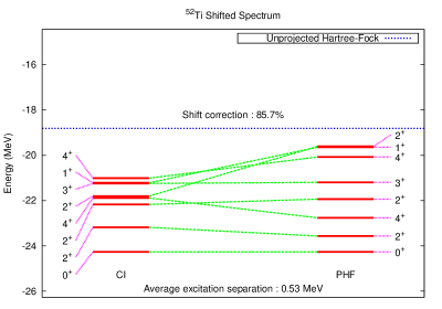
Figure 6: Comparison of exact CI and PHF spectra of ⁵²Ti in the $pf$ model space with the KB3G interaction, but with the PHF spectrum shifted downwards so the g.s. energies coincide.

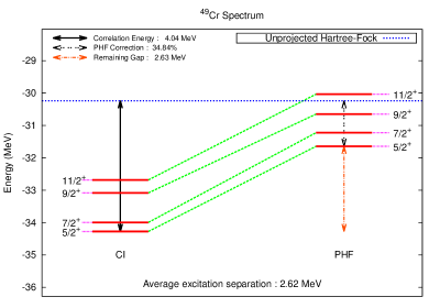
Figure 7: Comparison of exact CI and PHF spectra of ⁴⁹Cr in the $pf$ model space with the KB3G interaction.

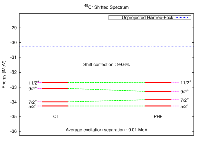
Figure 8: Comparison of exact CI and PHF spectra of ⁴⁹Cr in the $pf$ model space with the KB3G interaction, but with the PHF spectrum shifted downwards so the g.s. energies coincide.

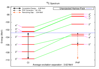
Figure 9: Comparison of exact CI and PHF spectra of ¹⁸C in the $p$-$sd_{5/2}$ model space.

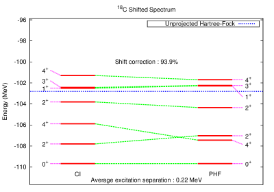
Figure 10: Comparison of exact CI and PHF spectra of ¹⁸C in the $p$-$sd_{5/2}$ model space, but with the PHF spectrum shifted downwards so the g.s. energies coincide.

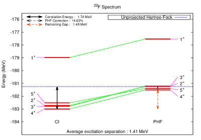
Figure 11: Comparison of exact CI and PHF spectra of ²²F in the $p$-$sd_{5/2}$ model space.

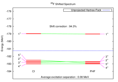
Figure 12: Comparison of exact CI and PHF spectra of ²²F in the $p$-$sd_{5/2}$ model space, but with the PHF spectrum shifted downwards so the g.s. energies coincide.

Table 1: Summary of data for the nuclei in the paper. The standard deviation is for the shifted PHF spectra relative to the exact CI spectra.

		Valence		Std. dev.	$\%$ PHF
Shell	Nucleus	Z	N	(MeV)	states
$sd$	24Mg	4	4	0.077	7
	30Al	5	9	1.004	12
$pf$	52Ti	2	10	0.714	8
	49Cr	4	5	0.074	4
$p$-$sd_{5/2}$	18C	4	10	0.810	7
	22F	7	11	0.194	5

Table 2: Frequency of ground state matching. The “No. nuclei” column represents the total number of nuclei that was studied for that shell that satisfies the Z-N relationship.

		No.	Correct	Incorrect	Frequency
Z - N	Shell	nuclei	G.S. $\mathbf{J}$	G.S. $\mathbf{J}$	correct
Even-Even	$s$-$d$	15	15	0	1.00
	$p$-$f$	10	10	0	1.00
	$p$-$sd$	17	12	5	0.71
Odd-Odd	$s$-$d$	15	8	7	0.53
	$p$-$f$	6	2	4	0.33
	$p$-$sd$	12	4	8	0.33
Odd-A	$s$-$d$	25	17	8	0.68
	$p$-$f$	11	6	5	0.55
	$p$-$sd$	25	13	12	0.52

VI Conclusions

We have carried out detailed angular momentum projected Hartree-Fock calculations in a shell-model basis with semi-realistic shell-model interactions, and compared the spectra to exact configuration-interaction diagonalization calculations, with a particular focus on the quality of the excitation spectra. We found, unsurprisingly, that rotational nuclei are best reproduced by PHF.

The U.S. Department of Energy supported this investigation through grant DE-FG02-96ER40985.

Appendix A Some computational details for Hartree-Fock

A single general Slater determinant we write as a rectangular, $N_{s}\times N_{p}$ matrix $\mathbf{\Psi}$. Operationally, the vectors $\vec{u}_{i}$, of length $N_{s}$, from solving the Hartree-Fock equation (6) form the columns of the transformation of the single-particle basis (3). We take the $N_{p}$ vectors with lowest $\epsilon_{\lambda}$ to form the columns of $\mathbf{\Psi}$. In other words, $\mathbf{\Psi}$ is simply selecting columns of $\mathbf{U}$, which are computed in Eq. (6); this is the unitary transformation that diagonalizes $\mathbf{h}$ . We have separate proton and neutron Slater determinants, $\mathbf{\Psi}_{\pi}$ and $\mathbf{\Psi}_{\nu}$.

From the Slater determinant we construct the one-body density matrix,

$$\rho_{ab}=\left\langle\Psi\left|\hat{\phi}^{\dagger}_{a}\hat{\phi}_{b}\right|\Psi\right\rangle=\sum_{i=1}^{N_{p}}\Psi_{ai}\Psi^{*}_{bi}.$$ (13)

We then construct the Hartree-Fock effective one-body Hamiltonian,

$$h_{ab}=H^{1}_{ab}+\sum_{cd}V_{ac,bd}\rho_{cd}.$$ (14)

Because we have two species, we have to take a little care. If our interaction is an isospin scalar, then

$$V^{pp}_{abcd}=V^{nn}_{abcd}=V^{T=1}_{abcd}$$ (15)

and

$$V^{pn}_{abcd}=\frac{1}{2}\left(V^{T=0}_{abcd}+V^{T=1}_{abcd}\right).$$ (16)

Here we have suppressed the obvious decoupling of angular momentum BG77 ; Edmonds .

Then the proton Hartree-Fock Hamiltonian is

$$h^{\pi}_{ab}=H^{1}_{ab}+\sum_{cd}V^{pp}_{ac,bd}\rho^{\pi}_{cd}+V^{pn}_{ac,bd}\rho^{\nu}_{cd}$$ (17)

and similarly for the neutron Hartree-Fock Hamiltonian.

Appendix B Some computational details for projected Hartree-Fock

We now have to compute $\langle\Psi|\hat{R}(\Omega)|\psi\rangle$ and $\langle\Psi|\hat{H}\hat{R}(\Omega)|\psi\rangle$, where $\hat{R}$ is the rotation operator. In our case

$$\hat{R}|\Psi\rangle\rightarrow\mathbf{R}\mathbf{\Psi}=\tilde{\mathbf{\Psi}}$$ (18)

where $\mathbf{\Psi}$ and $\tilde{\mathbf{\Psi}}$ are $N_{s}\times N_{p}$ matrices representing our original and rotated Slater determinants, respectively, and $\mathbf{R}$ is the square matrix the carries out the rotation. In our single-particle basis the matrix elements are straightforward:

$$R_{ab}=\langle j_{a}m_{a}|\hat{R}(\alpha,\beta,\gamma)|j_{b}m_{m}\rangle=\delta_{j_{a}j_{b}}{\cal D}^{j_{a}}_{m_{a},m_{b}}(\alpha,\beta,\gamma),$$ (19)

where ${\cal D}^{j}_{m^{\prime},m}$ is the Wigner $D$-matrix Edmonds .

Compute the matrix elements between two oblique Slater determinants is relatively straightforward Lang93 . First,

$$\langle\Psi|\hat{R}|{\Psi}\rangle=\langle\Psi|\tilde{\Psi}\rangle=\det\Psi^{\dagger}\tilde{\Psi}.$$ (20)

Calculation of the Hamiltonian (and other) expectation value requires the density matrix,

$$\rho^{\prime}_{ab}=\frac{\langle\Psi|\hat{\phi}^{\dagger}_{a}\hat{\phi}_{b}|\tilde{\Psi}\rangle}{\langle\Psi|\tilde{\Psi}\rangle}=\left[\tilde{\mathbf{\Psi}}\left(\mathbf{\Psi}^{\dagger}\tilde{\mathbf{\Psi}}\right)^{-1}\mathbf{\Psi}^{\dagger}\right]_{ba}$$ (21)

Then

$$\langle\Psi|\hat{H}|\tilde{\Psi}\rangle=\sum_{ab}H^{1}_{ab}\rho^{\prime}_{ab}+\sum_{abcd}V_{ab,cd}(\rho^{\prime}_{ac}\rho^{\prime}_{bd}-\rho^{\prime}_{ad}\rho^{\prime}_{bc})$$ (22)

Accounting for two species is straightforward. Note that even if our original Slater determinants were real, by rotating over all angle they can become complex.

We only project out good angular momentum. We could in principle project out exact isospin; to do this we would have to use a single Slater determinant containing both protons and neutrons and rotate in isospin space. We leave such a modification for future work.

Appendix C Linear algebra of projected states

In order to calculate the weights of the angular momentum-projected states in the Hartree-Fock state, we have to investigate in some detail the linear algebra of solving Eq (12).

Specifically, we want to expand the Hartree-Fock state

$$|HF\rangle=\sum_{\lambda}a_{\lambda}|\lambda\rangle.$$ (23)

Now each state $\lambda$ has definite $J$, but can be broken up into $M$-components. Thus we expand

$$|HF\rangle=\sum_{\lambda,M}a_{\lambda,M}|\lambda,M\rangle$$ (24)

and we ultimately want

$$|a_{\lambda}|^{2}=\sum_{M}|a_{\lambda,M}|^{2}.$$ (25)

As discussed above, we want to solve the generalized eigenvalue problem

$$\mathbf{\cal H}\vec{g}_{\lambda}=E_{\lambda}\mathbf{\cal N}\vec{g}_{\lambda}$$ (26)

Now because

$$\sum{JKM}\hat{P}^{J}_{K,M}=1$$ (27)

we have $\mathrm{tr}\,\mathbf{\cal N}=1$.

To solve the generalized eigenvalue problem we decompose the norm matrix, $\mathbf{\cal N}=\mathbf{\cal SS}^{\dagger}$, for example by Cholesky or by diagonalization. In general there will be a null space which we project out.

By creating $\mathbf{h}=\mathbf{\cal S}^{-1}\mathbf{\cal H}\mathbf{\cal S}^{-1\dagger}$ (and also projecting out the null space, to eliminate division by zero), we then solve the ordinary eigenvalue problem

$$\mathbf{h}\vec{v}_{\lambda}=E_{\lambda}\vec{v}_{\lambda}.$$ (28)

Of course, $|\vec{v}_{\lambda}|^{2}=1$. Furthermore, because of this, the vectors $\vec{g}_{\lambda}=mathbf{\cal S}^{-1\dagger}\vec{v}_{\lambda}$ are orthonormal with respect to the norm matrix, that is

$$\vec{g}^{\dagger}_{\lambda}\mathbf{\cal N}\vec{g}_{\mu}=\delta_{\lambda\mu}.$$ (29)

Another way to see this is to note that

$$|\lambda,JM\rangle=\sum_{K}\hat{P}^{J}_{M,K}|HF\rangle g_{K}(\lambda)$$ (30)

and because $\hat{P}^{2}=\hat{P}$ we automatically get (29).

As stated above, our ultimate goal is to compute $|a_{\lambda}|^{2}$. Towards this end, we note that

$$a_{\lambda,M}=\langle\lambda,JM|HF\rangle=\sum_{K}{\cal N}^{J}_{M,K}g_{K}(\lambda)$$ (31)

so that

$$|a_{\lambda}|^{2}=\sum_{M}|a_{\lambda,M}|^{2}=\sum_{K,K^{\prime}}g^{*}_{K}(\lambda)({\cal N}^{2})^{2}_{K,K^{\prime}}g_{K^{\prime}}(\lambda)=\vec{g}_{\lambda}^{\dagger}\mathbf{\cal N}^{2}\vec{g}_{\lambda}.$$ (32)

We can rewrite this as

$$|a_{\lambda}|^{2}=\vec{v}_{\lambda}^{\dagger}\mathbf{\cal S}^{\dagger}\mathbf{\cal S}\vec{v}_{\lambda}$$ (33)

which is what we want in convenient terms. To confirm this is correct, we compute

$$\sum_{\lambda}|a_{\lambda}|^{2}=\sum_{\lambda}\vec{v}_{\lambda}^{\dagger}\mathbf{\cal S}^{\dagger}\mathbf{\cal S}\vec{v}_{\lambda}=\mathrm{tr}\,\left(\mathbf{\cal S}\sum_{\lambda}\vec{v}_{\lambda}\vec{v}_{\lambda}^{\dagger}\mathbf{\cal S}^{\dagger}\right)$$ (34)

but using the completeness relation, the sum over $\lambda$ yields just 1, and we have

$$\mathrm{tr}\mathbf{\cal S}\mathbf{\cal S}^{\dagger}=\mathrm{tr}\,\mathbf{\cal N}=1$$ (35)

as we’d expect.

References

- (1) P. Ring and P. Shuck, The nuclear many-body problem (Springer-Verlag, New York 1980).
- (2) R. E. Peierls and J. Yoccuz, Proc. Phys. Soc. (London) A70, 381 (1957).
- (3) S. G. Nilsson, Mat. Fys. Medd. Dan. Vid. Selsk.29, No. 16 (1955); A. Bohr and B. R. Mottelson, Nuclear structure, volume II: nuclear deformations (W. A. Benjamin, New York, 1975).
- (4) R. D. Lawson, Theory of the nuclear shell model (Clarendon Press, Oxford, 1980).
- (5) J. P. Elliot, Proc. Roy. Soc. (London) A245, 128 (1958); J. P. Elliot, Proc. Roy. Soc. (London) A245, 562 (1958); I. Talmi, Simple models of complex nuclei (Harwood Academic Publishers, Chur, Switzerland, 1993).
- (6) K. Hara and Y. Sun, Int. J. Mod. Phys. E 4, 637 (1995); J.A. Sheikh and K. Hara, Phys. Rev. Lett. 82, 3968 (1999); Y.S. Chen and Z.C. Gao, Phys. Rev. C 63, 014314 (2001); J.A. Sheikh, Y. Sun and R. Palit, Phys. Lett. B 507, 115 (2001); Y. Sun, J.A. Sheikh and G.-L. Long, Phys. Lett. B 533, 253 (2002); Y. Sun and C.-L. Wu, Phys. Rev. C 68, 024315 (2003), p. 024315.
- (7) K. W. Schmid, F. Grümmer, and A. Faessler, Phys. Rev. C 29, 291 (1984); E. Bender, K. W. Schmid, and A. Faessler, Phys. Rev. C 52, 3002 (1995); K. W. Schmid, Prog. Part. Nucl. Phys. 52, 565 (2004).
- (8) Z.-C. Gao and M. Horoi, Phys. Rev. C 79, 014311 (2009); Z.-C. Gao, M. Horoi, and Y. S. Chen, Phys. Rev. C 80, 034325 (2009)
- (9) I. Stetcu, PhD. thesis, Louisiana State University, 2003, http://etd.lsu.edu/docs/available/etd-0702103-154150/
- (10) I. Stetcu and C.W. Johnson, Phys. Rev. C 66, 034301 (2002).
- (11) P.J. Brussard and P.W.M. Glaudemans, Shell-model applications in nuclear spectroscopy (North-Holland Publishing Company, Amsterdam 1977).
- (12) B. A. Brown and B. H. Wildenthal, Annu. Rev. Nucl. Part. Sci. 38, 29 (1988).
- (13) E. Caurier, G. Martinez-Pinedo, F. Nowacki, A. Poves, and A. P. Zuker, Rev. Mod. Phys. 77, 427 (2005).
- (14) C. W. Johnson, W. E. Ormand, and P. G. Krastev, arxiv:1303.0905.
- (15) R. R. Whitehead, A. Watt, B. J. Cole, and I. Morrison, Adv. Nucl. Phys. 9, 123 (1977).
- (16) A. R. Edmonds, Angular Momentum in Quantum Mechanics, (Princeton University Press, Princeton, 1960).
- (17) B.A. Brown and W.A. Richter, Phys. Rev. C 74 034315 (2006).
- (18) A. Poves, J. Sánchez-Solano, E. Caurier and F. Nowacki, Nucl. Phys. A 694, 157 2001.
- (19) S. Cohen and D. Kurath, Nucl. Phys. 73, 1 (1965).
- (20) B.H. Wildenthal, Prog. Part. Nucl. Phys. 11, 5 (1984).
- (21) D. J. Millener and D. Kurath, Nucl. Phys A 255, 315 (1975).
- (22) G. H. Lang, C. W. Johnson, S. E. Koonin, and W. E. Ormand, Phys. Rev. C 48, 1518 (1993).