A Nyström flavored Calderón Calculus of order three for two dimensional waves

Abstract

In this paper we present and test a full discretization of all elements of the Calderón Calculus (layer potentials and integral operators) for the Helmholtz equation in smooth closed curves in the plane. The resulting integral equations provide approximations of order three for all variables involved. Test are shown for a wide array of direct, indirect and combined field integral equation at fixed frequency and for a Convolution Quadrature based approximation in the time domain.

1 Introduction

This paper introduces and tests a fully discrete Calderón Calculus for two dimensional acoustic waves, time-harmonic and transient. We present a novel simultaneous discretization of the two layer potentials and four integral operators associated to the Helmholtz equation at fixed frequency on a collection of smooth non-intersecting parametrizable closed curves in the plane. The method’s vocation is simplicity, and we can assert with some confidence, that it will not be easy to find another instance of such a simple method of reasonable order (order three in all variables, in strong norms), with so little computational and programming requirements. We do not make any claims, though, on the ability of this method to work on problems at high frequencies, and we are by no means competitors of sophisticated high order methods that look for fine details in complicated geometries. We do, however, claim that the set of tools exposed in this paper works for many other integral operators (experiments on the Laplace equation have been carried out by the authors as a prototyping tool), and we are working on the extension of these ideas to some more general problems. It is important to emphasize that we are not discretizing a particular integral equation, so we are not worrying on whether one formulation is better than another, or whether there are resonances. As we show in the examples, the discrete operators and potentials can be used to build any of the best known direct, indirect, and combined field integral equations for exterior problems, as well as more complicated systems of integral equations for transmission problems. The time domain extension is carried out by using a variable complex frequency and the Convolution Quadrature technology of Christian Lubich [22, 2].

The method works in a relatively simple way. On a parametric curve, several sets of points and normal vectors are sampled. They are harvested using three staggered uniform grids in parameter space. One grid is used to create sources and two grids are used for simultaneous (averaged) observation. Once each curve is sampled at the discrete level, merging information to create a unified discrete set is an easy task. The second step is the automatic creation of potentials and operators using direct evaluations of the kernel functions: all numerical integration processes are done explicitly in the method, and all equations and right-hand sides are fully discrete. The ideas behind these methods go back to a very simple quadrature method of order two by Saranen and Schroderus [25], later generalized [5] and improved to third order of convergence [13]. The treatment of the associated hypersingular operator is surprisingly simple as well: using the integration by parts formula that is common to Galerkin discretizations of the hypersingular integral equation, the paper [12] found a collection of fully discrete discretizations of order one and two for this hypersingular equation. Some additional work allowed us to put together the first Calderón Calculus of order two in [11]. This set of discrete operators is heavily asymmetric and has the disadvantage of requiring sampling of second derivatives of the parametrization of the curve due to the evaluation of the double layer operator on its diagonal. The current set of methods mixes the discoveries of [11] and [13] to create a discrete set of order three that is even simpler than the order two collection.

The discrete set is, as a matter of fact, a Nyström (quadrature) discretization of the integral operators, avoiding evaluation of singular kernels on the diagonal, looking for superconvergent location of observation points, and mixing observation grids to partially symmetrize the method, and achieve order three. However, the method can be better understood as a full discretization, with carefully chosen low order numerical integration, of a non- conforming Petrov-Galerkin discretization of the integral operators. The methods will be tested on a wide set of integral equations for exterior and transmission problems, and on a time-domain scattering problem. We will also test condition numbers of the different formulations and the possibility of using Calderón preconditioning.

Some discussion on the literature

Nyström methods [24, 1] are the most popular choices for integral equations of the second kind. For integral equations of the second kind with smooth periodic kernels, the trapezoidal rule gives rise to a very powerful method which converges superalgebraically [19, Chapter 12]. Periodic weakly singular integral equations of the second kind (as those that arise from the Helmholtz equation on smooth parametrizable domains in the plane) are also amenable to simple methods with superalgebraic or exponential order of convergence [8, Section 3.5] (see also [20, 23]). A comparison of Nyström methods in the plane has been carried out in [16]. The three dimensional case is much more involved and consequently less developed. There are Nyström schemes for equations with weakly singular kernels, like those of Bruno and Kunyaski [4, 3] and Wienert [8, 27, 15]. Finally, the QBX methods [18, 14, 16], originally designed to compute layer potentials close to the boundary, are proving to be useful tools to create Nyström methods for weakly singular integral equations in two and three dimensions.

2 Parametrized Calderón Calculus

Let $\mathbf{x}:\mathbb{R}\to\Gamma\subset\mathbb{R}^{2}$ be a smooth ($\mathbf{x}\in\mathcal{C}^{\infty}(\mathbb{R})$) regular ($|\mathbf{x}^{\prime}(t)|\neq 0$ for all $t$) $1$-periodic ($\mathbf{x}(t+1)=\mathbf{x}(t)$ for all $t$) positively oriented parametrization of a simple ($\mathbf{x}(t)\neq\mathbf{x}(\tau)$ if $0\leq t<\tau<1$) closed curve in the plane. We consider the parametrized non-normalized normal vector field $\mathbf{n}(t):=(x_{2}^{\prime}(t),-x_{1}^{\prime}(t))$. The curve $\Gamma$ divides the plane into a bounded interior domain $\Omega_{-}$ and its unbounded exterior $\Omega_{+}$. Given a function $U:\mathbb{R}^{2}\setminus\Gamma\to\mathbb{C}$ that is smooth enough on both sides of the interface $\Gamma$, we will write $U^{\pm}$ for its restrictions of $\Omega_{\pm}$. Restrictions (traces) and normal derivatives on the boundary will be defined as:

$$\gamma^{\pm}U:=U^{\pm}|_{\Gamma}\circ\mathbf{x},\qquad\partial_{\mathbf{n}}^{\pm}U:=\big{(}(\nabla U^{\pm})|_{\Gamma}\circ\mathbf{x}\big{)}\cdot\mathbf{n}.$$ (2.1)

As defined, these restrictions to the boundary define periodic functions and that the normal derivative is actually a directional derivative with respect to the non-normalized outward pointing normal vector field $\mathbf{n}$.

Given complex valued sufficiently smooth $1$-periodic functions, we can define the single and double potentials on $\Gamma$ with the formulas

$$\big{(}\mathrm{S}\,\eta\big{)}(\mathbf{z}) := \frac{\imath}{4}\int_{0}^{1}H_{0}^{(1)}(k|\mathbf{z}-\mathbf{x}(t)|)\eta(t)\,\mathrm{d}t,$$ (2.2a)

$$\big{(}\mathrm{D}\,\psi\big{)}(\mathbf{z}) := \frac{\imath k}{4}\int_{0}^{1}H_{1}^{(1)}(k|\mathbf{z}-\mathbf{x}(t)|)\frac{(\mathbf{z}-{\bf x}(t))\cdot\mathbf{n}(t)}{|\mathbf{z}-\mathbf{x}(t)|}\psi(t)\,\mathrm{d}t.$$ (2.2b)

These functions are defined for all $\mathbf{z}\in\mathbb{R}^{d}\setminus\Gamma$. It is well known (it actually follows from a very simple computation) that for any $\eta,\psi$ the function $U:=\mathrm{S}\eta+\mathrm{D}\psi\in\mathcal{C}^{\infty}(\mathbb{R}^{2}\setminus\Gamma)$ solves

$$\Delta U+k^{2}U=0\mbox{ in $\mathbb{R}^{2}\setminus\Gamma$},\qquad\lim_{|\mathbf{z}|\to\infty}|\mathbf{z}|^{1/2}\Big{(}\nabla U(\mathbf{z})\cdot\big{(}{\textstyle\frac{1}{|\mathbf{z}|}}\,\mathbf{z}\big{)}-\imath\,k\,U(\mathbf{z})\Big{)}=0,$$ (2.3)

that is, $U$ is a radiating solution of the Helmholtz equation. Smoothness of $U$ as we approach the interface $\Gamma$ depends on smoothness of the densities $\eta$ and $\psi$. Reciprocally, given a solution of (2.3), we can write

$$U=\mathrm{S}[\![\partial_{\mathbf{n}}U]\!]-\mathrm{D}[\![\gamma U]\!],$$ (2.4)

where the jump operators are defined as

$$[\![\gamma U]\!]:=\gamma^{-}U-\gamma^{+}U,\qquad[\![\partial_{\mathbf{n}}U]\!]:=\partial_{\mathbf{n}}^{-}U-\partial_{\mathbf{n}}^{+}U.$$

Uniqueness of the representation (2.4) for the solutions of (2.3) implies the jump relations of potentials

$$[\![\gamma\mathrm{S}\,\eta]\!]=0,\qquad[\![\partial_{\mathbf{n}}\mathrm{S}\,\eta]\!]=\eta,\qquad[\![\gamma\mathrm{D}\psi]\!]=-\psi,\qquad[\![\partial_{\mathbf{n}}\mathrm{D}\psi]\!]=0.$$ (2.5)

These jump properties motivate the introduction of the four operators on the boundary $\Gamma$:

$$\mathrm{V}\eta:=\{\!\!\{\gamma\mathrm{S}\,\eta\}\!\!\}=\gamma^{\pm}\mathrm{S}\eta, \mathrm{J}\,\eta:=\{\!\!\{\partial_{\mathbf{n}}\mathrm{S}\,\eta\}\!\!\},$$ (2.6a)

$$\mathrm{K}\,\psi:=\{\!\!\{\gamma\mathrm{D}\,\psi\}\!\!\}, \mathrm{W}\psi:=-\{\!\!\{\partial_{\mathbf{n}}\mathrm{D}\,\psi\}\!\!\}=-\partial_{\mathbf{n}}^{\pm}\mathrm{D}\,\psi,$$ (2.6b)

where

$$\{\!\!\{\gamma U\}\!\!\}:={\textstyle\frac{1}{2}}(\gamma^{-}U+\gamma^{+}U),\qquad\{\!\!\{\partial_{\mathbf{n}}U\}\!\!\}:={\textstyle\frac{1}{2}}(\partial_{\mathbf{n}}^{-}U+\partial_{\mathbf{n}}^{+}U).$$

The operators $\mathrm{V}$ and $\mathrm{K}$ are the single and double layer operators respectively, $\mathrm{J}$ is the adjoint double layer operator, and $\mathrm{W}$ is the hypersingular operator for the Helmholtz equation. The first three of these operators admit integral expressions:

$$({\mathrm{V}}\eta)(\tau) := \frac{\imath}{4}\int_{0}^{1}H_{0}^{(1)}(k|\mathbf{x}(\tau)-{\mathbf{x}}(t)|)\eta(t)\,\mathrm{d}t,$$ (2.7a)

$$(\mathrm{K}\psi)(\tau) := \frac{\imath k}{4}\int_{0}^{1}H_{1}^{(1)}(k|\mathbf{x}(\tau)-\mathbf{x}(t)|)\frac{(\mathbf{x}(\tau)-{\bf x}(t))\cdot\mathbf{n}(t)}{|\mathbf{x}(\tau)-\mathbf{x}(t)|}\psi(t)\,\mathrm{d}t,$$ (2.7b)

$$(\mathrm{J}\eta)(\tau) := \frac{\imath k}{4}\int_{0}^{1}H_{1}^{(1)}(k|\mathbf{x}(\tau)-\mathbf{x}(t)|)\frac{(\mathbf{x}(t)-{\bf x}(\tau))\cdot\mathbf{n}(\tau)}{|\mathbf{x}(\tau)-\mathbf{x}(t)|}\eta(t)\,\mathrm{d}t.$$ (2.7c)

It is clear from here that $$\mathrm{J}=\mathrm{K}^{t} \mathrm{W}$$. We will keep a different notation though, for reasons that will become apparent when we discretize them in a non–symmetric form. The operator admits an expression in the form of an integro-differential operator:

$$\mathrm{W}\psi:=-(\mathrm{V}\psi^{\prime})^{\prime}-k^{2}\mathrm{V}_{\mathbf{n}}\psi,$$ (2.7d)

where

$$(\mathrm{V}_{\mathbf{n}}\psi)(\tau):=\frac{\imath}{4}\int_{0}^{1}H_{0}^{(1)}(k|\mathbf{x}(\tau)-{\bf x}(t)|)\big{(}\mathbf{n}(t)\cdot\mathbf{n}(\tau)\big{)}\psi(t)\,\mathrm{d}t.$$ (2.7e)

The representation formula (2.4) for all radiating solutions of the Helmholtz equation (2.3), together with the jump properties of the potentials (2.5) and the definitions of the boundary integral operators by averaging (2.6), determines a set of rules (a calculus) that generates a diverse collection of representation formulas, potential ansatzs, and integral equations associated to the solution of interior, exterior and transmission problems for the Helmholtz equation. The following matrices of operators

$$\left[\begin{array}[]{c}\gamma^{\pm}\\ \partial_{\mathbf{n}}^{\pm}\end{array}\right]\left[\begin{array}[]{cc}\mathrm{D}&-\mathrm{S}\end{array}\right]=\pm\frac{1}{2}\left[\begin{array}[]{cc}\mathrm{I}&0\\ 0&\mathrm{I}\end{array}\right]+\left[\begin{array}[]{cc}\mathrm{K}&-\mathrm{V}\\ -\mathrm{W}&-\mathrm{J}\end{array}\right]$$ (2.8)

collect the exterior/interior Cauchy values of the layer potentials. They constitute the exterior/interior Calderón projectors associated to the Helmholtz equation. The systematic use of these potentials and operators to build integral equations will be explored in Section 6. At this point, let us emphasize the fact that we are striving for a full discretization of the entire set of potentials (2.2) and operators (2.7), including also discretization of the restriction operators (2.1) that will be needed to sample, at the discrete level, incoming incident waves.

The case of multiple scatterers

Assume that $\Gamma_{1},\ldots,\Gamma_{M}$ are pairwise disjoint curves, parametrized as above by smooth $1$-periodic functions $\mathbf{x}_{\ell}$. All potentials and operators can be easily defined for vectors of densities $(\eta_{1},\ldots,\eta_{M})$ and $(\psi_{1},\ldots,\psi_{M})$. The integral operators then become matrices of integral operators. For instance, we have operators of the form

$$\frac{\imath}{4}\int_{0}^{1}H_{0}^{(1)}(k|\mathbf{x}_{\ell}(\tau)-{\mathbf{x}_{m}}(t)|)\eta_{m}(t)\,\mathrm{d}t,\qquad\ell,m=1,\ldots,M.$$

3 Fully discrete method

3.1 Geometry

For one single curve parametrized with $\mathbf{x}$ as in Section 2, we proceed as follows. We take a positive integer $N$ and define $h:=1/N$. Next we define the discrete parameter points $t_{j}:=h\,j$ and the values

$$\mathbf{m}_{j}:=\mathbf{x}(t_{j}),\quad\mathbf{b}_{j}:=\mathbf{x}(t_{j}-h/2),\quad\mathbf{n}_{j}:=h\,\mathbf{n}(t_{j}),\quad j\in\mathbb{Z}_{N}:=\{1,\ldots,N\}.$$

The notation $\mathbf{m}_{j}$ and $\mathbf{b}_{j}$ makes reference to midpoints and breakpoints of a boundary element mesh that is implicit to this method (see Section 4). In addition to these sampled quantities, we need two index-based functions that provide the next and previous index modulo $N$: the next-index function is $n:\mathbb{Z}_{N}\to\mathbb{Z}_{N}$ given by

$$n(j):=\left\{\begin{array}[]{ll}j+1,&1\leq j\leq N-1,\\ 1,&j=N,\end{array}\right.$$

while $p:=n^{-1}$. Merging geometric information from several curves is easy: after sampling two curves $\Gamma_{1}$ and $\Gamma_{2}$ with $N_{1}$ and $N_{2}$ elements respectively, midpoints, breakpoints, and normals are collected in lists with $N=N_{1}+N_{2}$ elements, by appending the information of $\Gamma_{2}$ after the information of $\Gamma_{1}$. We then create the next-index and previous-index functions by juxtaposing the two existing functions:

$$n(j)=\left\{\begin{array}[]{ll}j+1,&1\leq j\leq N_{1}-1,\\ 1,&j=N_{1},\\ j+1,&N_{1}+1\leq j\leq N_{1}+N_{2}-1,\\ N_{1}+1,&j=N_{1}+N_{2},\end{array}\right.\qquad p=n^{-1}.$$

This merging process can be applied to any finite number of curves, each one discretized (sampled) with a different number of points. The quantity $h$ appears only at the time of collecting information from a particular curve and is incorporated to quantities related to first derivatives of the parametrization. However, at the time of merging, $h$ is absent from any expression. From this moment on, $n:\mathbb{Z}_{N}\to\mathbb{Z}_{N}$ is a permutation of $\mathbb{Z}_{N}$ and $p=n^{-1}.$

3.2 Discrete potentials

The discrete version of the single and double layer potentials (2.2) is defined by using linear combinations of monopoles and dipoles:

$$\Phi_{j}(\mathbf{z}):=\frac{\imath}{4}H^{(1)}_{0}(k|\mathbf{z}-\mathbf{m}_{j}|)\qquad\mbox{and}\qquad D_{j}(\mathbf{z}):=\frac{\imath k}{4}H^{(1)}_{1}(k|\mathbf{z}-\mathbf{m}_{j}|)\frac{(\mathbf{z}-\mathbf{m}_{j})\cdot\mathbf{n}_{j}}{|\mathbf{z}-\mathbf{m}_{j}|}.$$

Given two vectors $\bm{\eta}=(\eta_{1},\ldots,\eta_{N})^{\top},\bm{\psi}=(\psi_{1},\ldots,\psi_{N})^{\top}\in\mathbb{C}^{N}$, the discrete potentials

$$\mathrm{S}_{h}(\mathbf{z})\bm{\eta} := \sum_{j=1}^{N}\eta_{j}\Phi_{j}(\mathbf{z}),$$ (3.1a)

$$\mathrm{D}_{h}(\mathbf{z})\bm{\psi} := {\textstyle\frac{1}{24}}\sum_{j=1}^{N}\psi_{j}(D_{p(j)}(\mathbf{z})+22D_{j}(\mathbf{z})+D_{n(j)}(\mathbf{z}))$$

$$= {\textstyle\frac{1}{24}}\sum_{j=1}^{N}(\psi_{p(j)}+22\psi_{j}+\psi_{n(j)})D_{j}(\mathbf{z}),$$

define solutions of (2.3).

A quadrature related matrix

Let us consider the $N\times N$ matrix $\mathrm{Q}$ given by

$$\mathrm{Q}_{i,i}={\textstyle\frac{11}{12}},\qquad\mathrm{Q}_{i,n(i)}=\mathrm{Q}_{i,p(i)}={\textstyle\frac{1}{24}},\qquad\mathrm{Q}_{i,j}=0\quad\mbox{otherwise.}$$ (3.2)

When the geometry proceeds from a single sampled curve, and therefore the next-index function is just a right-shift modulo $N$, $\mathrm{Q}$ is the circulant symmetric matrix

$$\mathrm{Q}=\frac{1}{24}\left[\begin{array}[]{ccccc}22&1&&&1\\ 1&22&1&&\\ &\ddots&\ddots&\ddots\\ &&1&22&1\\ 1&&&1&22\end{array}\right].$$

In general, $\mathrm{Q}$ is block diagonal with blocks of the above form, one for each of the curves. This matrix is related to a quadrature formula that will be introduced in Section 4. It is clear that (3.1) is just a linear combination of dipoles, where either the coefficients are premultiplied by the matrix $\mathrm{Q}$, or the dipoles themselves are mixed using this matrix.

3.3 Observation grids and mixing matrices

Since the integral operators in (2.7) have singularities at $\tau=t$, we are forced to use a different discrete set for testing. We start by defining two sets of discrete samples. For a single curve parametrized with $\mathbf{x}$, we use the same $N$ and $h=1/N$ to define

$$\mathbf{m}_{j}^{\pm}:=\mathbf{x}(t_{j}\pm h/6),\quad\mathbf{b}_{j}^{\pm}:=\mathbf{x}(t_{j}-h/2\pm h/6),\quad\mathbf{n}_{j}^{\pm}:=h\,\mathbf{x}(t_{j}\pm h/6),\quad j\in\mathbb{Z}_{N}.$$

As in Section 3.1, observations on finite collections of curves are merged in a simple way. We demand that the number of discretization and observation points on each curve coincides, although it can be taken to be different on different curves.

Instead of directly averaging values from both possible choices, we will be considering a more general mixture of the two grids. We start with the $N\times N$ matrix $\mathrm{P}^{+}=\mathrm{P}^{+}(\alpha)$ with elements

$$\mathrm{P}^{+}_{i,i}:={\textstyle\frac{1}{2}}\alpha,\qquad\mathrm{P}_{i,p(i)}^{+}:={\textstyle\frac{1}{2}}(1-\alpha),\qquad\mathrm{P}^{+}_{i,j}=0\quad\mbox{otherwise}.$$

The parameter $\alpha>0$ will be discussed in Section 5. We also let $\mathrm{P}^{-}:=(\mathrm{P}^{+})^{\top}$. For the case of a single curve (when $n$ is the right-shift modulo $N$), we show two particular cases of interest:

$$\mathrm{P}^{+}({\textstyle\frac{5}{6}})=\frac{1}{12}\left[\begin{array}[]{cccc}5&&&1\\ 1&5\\ &\ddots&\ddots\\ &&1&5\end{array}\right],\qquad\mathrm{P}^{+}(1)={\textstyle\frac{1}{2}}\mathrm{I}.$$

Given two vectors $\bm{\xi}^{\pm}\in\mathbb{C}^{N}$, it is easy to see that

$$(\mathrm{P}^{+}\bm{\xi}^{+}+\mathrm{P}^{-}\bm{\xi}^{-})_{i}={\textstyle\frac{1}{2}}((1-\alpha)\xi^{+}_{p(i)}+\alpha\xi_{i}^{-}+\alpha\xi_{i}^{+}+(1-\alpha)\xi_{n(i)}^{-}).$$ (3.3)

Similarly, the $i$-th element of $\mathrm{Q}(\mathrm{P}^{+}\bm{\xi}^{+}+\mathrm{P}^{-}\bm{\xi}^{-})=\mathrm{P}^{+}\mathrm{Q}\bm{\xi}^{+}+\mathrm{P}^{-}\mathrm{Q}\bm{\xi}^{-}$, namely

$${\textstyle\frac{1}{48}}\Big{(}(1-\alpha)\xi_{p^{2}(i)}^{+}+\alpha\xi_{p(i)}^{-}+(22-21\alpha)\xi_{p(i)}^{+}+(21\alpha+1)\xi_{i}^{-}$$

$$+(21\alpha+1)\xi_{i}^{+}+(22-21\alpha)\xi^{-}_{n(i)}+\alpha\xi^{+}_{n(i)}+(1-\alpha)\xi^{-}_{n^{2}(i)}\Big{)},$$ (3.4)

is a weighted local average of the values around the index $i$.

The testing part of the discrete Calderón Calculus is applied upon an incident wave. At this point, this is just a function $U^{\mathrm{inc}}:\mathbb{R}^{2}\to\mathbb{C}$ that is smooth around the collection of curves, so that we can evaluate

$$\bm{\beta}_{0}^{\pm} := -(U^{\mathrm{inc}}(\mathbf{m}_{1}^{\pm}),\ldots,U^{\mathrm{inc}}(\mathbf{m}_{N}^{\pm}))^{\top},$$ (3.5a)

$$\bm{\beta}_{1}^{\pm} := -(\nabla U^{\mathrm{inc}}(\mathbf{m}_{1}^{\pm})\cdot\mathbf{n}_{1}^{\pm},\ldots,\nabla U^{\mathrm{inc}}(\mathbf{m}_{N}^{\pm})\cdot\mathbf{n}_{N}^{\pm})^{\top}.$$ (3.5b)

We finally define the observation of the incident wave and its normal derivative with

$$\bm{\beta}_{0}:=\mathrm{P}^{+}\bm{\beta}_{0}^{+}+\mathrm{P}^{-}\bm{\beta}^{-}_{0},\qquad\bm{\beta}_{1}:=\mathrm{Q}(\mathrm{P}^{+}\bm{\beta}_{1}^{+}+\mathrm{P}^{-}\bm{\beta}^{-}_{1}).$$ (3.5c)

3.4 Discrete operators

The discrete operators are defined using the geometric elements of Section 3.1 in the integration variable and the observation grids of Section 3.3 in the test variable. The subscript $h$ will be used to denote discretization. In the case of several curves $\{\Gamma_{1},\ldots,\Gamma_{M}\}$, we can consider that $h:=(1/N_{1},\ldots,1/N_{M})$, although this is not relevant for the exposition of the methods.

Following (2.7) we define two sets of discrete operators (based on the principal sampling of the geometry, tested on both $\pm$ observation grids). We start with the three integral operators

$$\mathrm{V}_{i,j}^{\pm} := \frac{\imath}{4}H^{(1)}_{0}(k|\mathbf{m}_{i}^{\pm}-\mathbf{m}_{j}|),$$ (3.6a)

$$\mathrm{K}_{i,j}^{\pm} := \frac{\imath\,k}{4}H^{(1)}_{1}(k|\mathbf{m}_{i}^{\pm}-\mathbf{m}_{j}|)\frac{(\mathbf{m}_{i}^{\pm}-\mathbf{m}_{j})\cdot\mathbf{n}_{j}}{|\mathbf{m}_{i}^{\pm}-\mathbf{m}_{j}|},$$ (3.6b)

$$\mathrm{J}_{i,j}^{\pm} := \frac{\imath\,k}{4}H^{(1)}_{1}(k|\mathbf{m}_{j}-\mathbf{m}_{i}^{\pm}|)\frac{(\mathbf{m}_{j}-\mathbf{m}_{i}^{\pm})\cdot\mathbf{n}_{i}^{\pm}}{|\mathbf{m}_{j}-\mathbf{m}_{i}^{\pm}|}.$$ (3.6c)

Following (2.7d), the discretization of $$\mathrm{W}$$ separates the discretization of the principal part

$$\widetilde{\mathrm{W}}_{i,j}^{\pm}:=\widetilde{\mathrm{V}}^{\pm}_{n(i),n(j)}-\widetilde{\mathrm{V}}^{\pm}_{n(i),j}-\widetilde{\mathrm{V}}^{\pm}_{i,n(j)}+\widetilde{\mathrm{V}}^{\pm}_{i,j},\qquad\widetilde{\mathrm{V}}^{\pm}_{i,j}:=\frac{\imath}{4}H^{(1)}_{0}(k|\mathbf{b}_{i}^{\pm}-\mathbf{b}_{j}|),$$ (3.6d)

from the more regular logarithmic term in (2.7e)

$$\mathrm{V}_{\mathbf{n},i,j}^{\pm}:=(\mathbf{n}_{i}^{\pm}\cdot\mathbf{n}_{j})\mathrm{V}_{i,j}^{\pm}.$$ (3.6e)

If $\mathrm{V}^{\pm}_{h},\mathrm{K}^{\pm}_{h},\mathrm{J}^{\pm}_{h},\widetilde{\mathrm{W}}^{\pm}_{h},$ and $\mathrm{V}_{\mathbf{n},h}^{\pm}$ are the above matrices, we define the matrices of the discrete Calderón Calculus by

$$\mathrm{V}_{h} := \mathrm{P}^{+}\mathrm{V}_{h}^{+}+\mathrm{P}^{-}\mathrm{V}_{h}^{-},$$ (3.7a)

$$\mathrm{K}_{h} := \mathrm{P}^{+}\mathrm{K}^{+}_{h}\mathrm{Q}+\mathrm{P}^{-}\mathrm{K}^{-}_{h}\mathrm{Q}=(\mathrm{P}^{+}\mathrm{K}^{+}_{h}+\mathrm{P}^{-}\mathrm{K}^{-}_{h})\mathrm{Q},$$ (3.7b)

$$\mathrm{J}_{h} := \mathrm{P}^{+}\mathrm{Q}\mathrm{J}_{h}^{+}+\mathrm{P}^{-}\mathrm{Q}\mathrm{J}^{-}_{h}=\mathrm{Q}(\mathrm{P}^{+}\mathrm{J}_{h}^{+}+\mathrm{P}^{-}\mathrm{J}^{-}_{h})$$ (3.7c)

$$\mathrm{W}_{h} := \mathrm{P}^{+}\widetilde{\mathrm{W}}^{+}_{h}+\mathrm{P}^{-}\widetilde{\mathrm{W}}^{-}_{h}-k^{2}(\mathrm{P}^{+}\mathrm{Q}\mathrm{V}_{\mathbf{n},h}^{+}\mathrm{Q}+\mathrm{P}^{-}\mathrm{Q}\mathrm{V}_{\mathbf{n},h}^{-}\mathrm{Q})$$ (3.7d)

$$= \mathrm{P}^{+}\widetilde{\mathrm{W}}^{+}_{h}+\mathrm{P}^{-}\widetilde{\mathrm{W}}^{-}_{h}-k^{2}\mathrm{Q}(\mathrm{P}^{+}\mathrm{V}_{\mathbf{n},h}^{+}+\mathrm{P}^{-}\mathrm{V}_{\mathbf{n},h}^{-})\mathrm{Q}.$$ (3.7e)

The Calderón projectors (2.8) include the action of two identity operators. Both of them will be approximated by the following mass matrix $\mathrm{M}=\mathrm{M}(\alpha)$

$$\mathrm{M}_{i,i}:={\textstyle\frac{2}{9}}(1+3\alpha),\quad\mathrm{M}_{i,p(i)}=\mathrm{M}_{i,n(i)}:={\textstyle\frac{1}{18}}(7-6\alpha),\quad\mathrm{M}_{i,j}=0\quad\mbox{otherwise}.$$ (3.8)

The simplest method corresponds to $\alpha=1$. In this case $\mathrm{P}^{\pm}=\frac{1}{2}\,\mathrm{I}$ and, apart from the action of the matrix $\mathrm{Q}$ (related to quadrature), we are just averaging sets of equations on the two grids. However, even in this simple case, the mass matrix has a circulant tridiagonal structure.

4 From Nyström to Petrov-Galerkin

In this section we reinterpret all the matrices and testing of right-hand sides given in Section 3 as non-conforming Petrov-Galerkin method with numerical quadrature. This will be done for the case of a single curve, where we are working with a single equation and parametric unit interval ($1$-periodic real line). When there are $M$ curves, $M$ copies of the unit interval have to be used. The details just became slightly more cumbersome, but all the following arguments can be extended readily.

Discrete functions and spaces

We start by setting some notation. Given $z\in\mathbb{R}$, we write $\delta_{z}$ to denote the $1$-periodic Dirac delta distribution at $z$, that is, the Dirac comb supported on $z+\mathbb{Z}$. Given an open interval $I$, of length less than one, we write $\chi_{I}$ to denote the $1$-periodic function that coincides with the characteristic function of $I$ on a unit length interval containing $I$. We then write

$$\delta_{i}:=\delta_{t_{i}},\quad\delta_{i}^{\pm}:=\delta_{t_{i}\pm h/6},\quad\chi_{i}:=\chi_{(t_{i}-h/2,t_{i}+h/2)},\quad\chi_{i}^{\pm}:=\chi_{(t_{i}\pm h/6-h/2,t_{i}\pm h/6+h/2)}.$$

Next we define the Dirac fork (see (3.3) to recognize the corresponding coefficients)

$$\delta_{i}^{\star}:={\textstyle\frac{1}{2}}\Big{(}(1-\alpha)\delta_{i-1}^{+}+\alpha\delta_{i}^{-}+\alpha\delta_{i}^{+}+(1-\alpha)\delta_{i+1}^{-}\Big{)},$$ (4.1)

and the ziggurat-shaped piecewise constant functions

$$\chi_{i}^{\star}:={\textstyle\frac{1}{2}}\Big{(}(1-\alpha)\chi_{i-1}^{+}+\alpha\chi_{i}^{-}+\alpha\chi_{i}^{+}+(1-\alpha)\chi_{i+1}^{-}\Big{)}.$$ (4.2)

Figure 1 shows the shapes of the basic test functions for the particular case $\alpha=5/6$. Using momentarily the notation $s_{i}^{\pm}:=t_{i}-h/2\pm h/6$, it is easy to note that, in the sense of periodic distributions,

$${\textstyle\frac{\mathrm{d}}{\mathrm{d}t}}\chi_{i}^{\pm}=\delta_{s_{i}^{\pm}}-\delta_{s_{i+1}^{\pm}}$$

and

$${\textstyle\frac{\mathrm{d}}{\mathrm{d}t}}\chi_{i}^{\star} = {\textstyle\frac{1}{2}}\Big{(}(1-\alpha)\delta_{s_{i-1}^{+}}+\alpha\delta_{s_{i}^{-}}+\alpha\delta_{s_{i}^{+}}+(1-\alpha)\delta_{s_{i+1}^{-}}\Big{)}$$

$$-{\textstyle\frac{1}{2}}\Big{(}(1-\alpha)\delta_{s_{i}^{+}}+\alpha\delta_{s_{i+1}^{-}}+\alpha\delta_{s_{i+1}^{+}}+(1-\alpha)\delta_{s_{i+2}^{-}}\Big{)}.$$

This shows how, in the same way that characteristic functions arise from integrating two consecutive deltas with opposite signs, the ziggurat functions arise from integrating Dirac forks. Four spaces are relevant for what follows:

$$T_{h}:=\mathrm{span}\{\delta_{i}\,:\,i\in\mathbb{Z}_{N}\}, T_{h}^{\star}:=\mathrm{span}\{\delta_{i}^{\star}\,:\,i\in\mathbb{Z}_{N}\},$$ (4.3a)

$$S_{h}:=\mathrm{span}\{\chi_{i}\,:\,i\in\mathbb{Z}_{N}\}, S_{h}^{\star}:=\mathrm{span}\{\chi_{i}^{\star}\,:\,i\in\mathbb{Z}_{N}\}.$$ (4.3b)

Note that $S_{h}$ is just the space of periodic piecewise constant functions on a uniform mesh with mesh-size $h$ and $\{t_{i}\}$ as midpoints of the mesh elements. The $T$ spaces will be non-conforming discretizations of $H^{-1/2}$ Sobolev spaces, while the $S$ spaces are non-conforming approximations of $H^{1/2}$. The $\star$ spaces will do the job of test spaces, while the unscripted spaces will be the trial spaces.

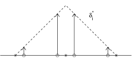
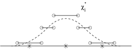
Figure 1: The shape of the combination of Dirac deltas $\delta_{i}^{\star}$ and the piecewise constant function $\chi_{i}^{\star}$. The plot is given for the choice $\alpha=5/6$. A piecewise linear function and a quadratic spline are shown in the background. They are at the origin of the choice of coefficients for the distribution $\delta_{i}^{\star}$.

Interactions of deltas and characteristic functions

We define the actions of deltas with characteristic functions with the formulas

$$\langle\chi_{i}^{\pm},\delta_{i}\rangle :=\alpha+{\textstyle\frac{1}{12}} =:\langle\delta_{i}^{\pm},\chi_{i}\rangle,$$ (4.4a)

$$\langle\chi_{i+1}^{-},\delta_{i}\rangle=\langle\chi_{i-1}^{+},\delta_{i}\rangle :={\textstyle\frac{11}{12}}-\alpha =:\langle\delta_{i-1}^{+},\chi_{i}\rangle=\langle\delta_{i+1}^{-},\chi_{i}\rangle,$$ (4.4b)

$$\langle\delta_{i},\chi_{j}^{\pm}\rangle :=0 =:\langle\delta_{j}^{\pm},\chi_{i}\rangle,\hskip 56.9055pt\mbox{otherwise}.$$ (4.4c)

The otherwise case above has to be understood modulo $N$. This interaction will be explained in Section 5. It is clear that the first line of (4.4) enforces the second, if we want some kind of consistency of our formulas with respect to translations in the origin of the real line. The interactions (4.4) and the definitions (4.1), (4.2) imply that (see (3.8))

$$\langle\delta_{i}^{\star},\chi_{i}\rangle=\langle\chi_{i}^{\star},\delta_{i}\rangle ={\textstyle\frac{2}{9}}(1+3\alpha)=\mathrm{M}_{i,i},$$

$$\langle\delta_{i\pm 1}^{\star},\chi_{i}\rangle=\langle\chi_{i\pm 1}^{\star},\delta_{i}\rangle ={\textstyle\frac{1}{18}}(7-6\alpha)=\mathrm{M}_{i,i\pm 1}=\mathrm{M}_{i\pm 1,i},$$

$$\langle\delta_{i}^{\star},\chi_{j}\rangle=\langle\chi_{i}^{\star},\delta_{j}\rangle =0,\hskip 28.45274pt\mbox{otherwise}.$$

In other words, the matrix $\mathrm{M}$ is the matrix that represents the ‘dualities’ $S_{h}^{\star}\times T_{h}$ and $T_{h}^{\star}\times S_{h}$ if (4.4) is imposed. It is to be noticed that in the simplest case ($\alpha=1$), the interaction of a Dirac delta with a characteristic function is forced to be negative on neighboring elements (4.4b). We will discuss these choices in Section 5.

First collection of discrete elements

While the angled bracket (linear in both components) is used for the concrete interactions of piecewise constant functions and Dirac delta distributions, from now on we will use curly brackets (linear in both components as well) for the following situations

$$\{\delta_{z},\phi\}:=\phi(z),\qquad\{\chi_{I},\phi\}:=\int_{I}\phi(t)\mathrm{d}t.$$

This can be applied as long as the right-hand side of the expression is meaningful. We can then define the following bilinear forms

$$T_{h}^{\star}\times T_{h}\ni(\mu_{h}^{\star},\eta_{h}) \longmapsto\quad \{\mu_{h}^{\star},\mathrm{V}\eta_{h}\},$$ (4.5a)

$$S_{h}^{\star}\times S_{h}\ni(\phi_{h}^{\star},\psi_{h}) \longmapsto\quad \{{\textstyle\frac{\mathrm{d}}{\mathrm{d}t}}\phi_{h}^{\star},\mathrm{V}{\textstyle\frac{\mathrm{d}}{\mathrm{d}t}}\psi_{h}\},$$ (4.5b)

as well as the linear map

$$T_{h}^{\star}\ni\mu_{h}^{\star}\quad\longmapsto\quad\{\mu_{h}^{\star},U^{\mathrm{inc}}\circ\mathbf{x}\}.$$ (4.5c)

With the given bases for the spaces (4.3), the bilinear forms produce the matrix $\mathrm{V}_{h}$ and $\mathrm{P}^{+}\widetilde{\mathrm{W}}^{+}_{h}+\mathrm{P}^{-}\widetilde{\mathrm{W}}^{-}_{h}$, while the linear form yields the vector $\bm{\beta}_{0}$.

Look around quadrature

What is missing to get a complete discrete set is the full discretization of the following bilinear forms

$$T_{h}^{\star}\times S_{h}\ni(\mu_{h}^{\star},\psi_{h}) \longmapsto\quad \{\mu_{h}^{\star},\mathrm{K}\psi_{h}\},$$ (4.6a)

$$S_{h}^{\star}\times T_{h}\ni(\phi_{h}^{\star},\eta_{h}) \longmapsto\quad \{\phi_{h}^{\star},\mathrm{J}\eta_{h}\},$$ (4.6b)

$$S_{h}^{\star}\times S_{h}\ni(\phi_{h}^{\star},\psi_{h}) \longmapsto\quad \{\phi_{h}^{\star},\mathrm{V}_{\mathbf{n}}\psi_{h}\},$$ (4.6c)

and the linear form

$$S_{h}^{\star}\ni\phi_{h}^{\star}\quad\longmapsto\quad\{\phi_{h}^{\star},(\nabla U^{\mathrm{inc}}\circ\mathbf{x})\cdot\mathbf{n}\}.$$ (4.6d)

The elements of the space $S_{h}^{\star}$, can be decomposed as sums of elements of the spaces

$$S_{h}^{\pm}:=\mathrm{span}\{\chi_{i}^{\pm}\;:\,i\in\mathbb{Z}_{N}\}.$$

Therefore, the practical computation of all elements in (4.6) can be done if we are able to compute integrals of the form

$$\int_{a-h/2}^{a+h/2}\mathbf{f}(t)\cdot\mathbf{n}(t)\mathrm{d}t,\qquad\int_{a-h/2}^{a+h/2}\int_{b-h/2}^{b+h/2}m(t,\tau)\,\mathbf{n}(t)\cdot\mathbf{n}(\tau)\mathrm{d}t\mathrm{d}\tau.$$ (4.7)

The approximation of integrals in one variable will be carried out with a three-point formula of order four using points outside the integration interval (see (3.2))

$$\int_{a-h/2}^{a+h/2}\phi(t)\mathrm{d}t\approx\frac{h}{24}(\phi(a-h)+22\phi(a)+\phi(a+h)).$$ (4.8)

Second collection of discrete elements

As already mentioned, the semidiscrete elements (4.6) can be fully discretized once we approximate all integrals of the form (4.7). For the one variable integrals we use (4.7) and for the double integrals we use the nine-point formula that arises from using (4.8) in each variable. Note that the normal vector appears always in the integration variable and that we have defined $\mathbf{n}_{i}:=h\,\mathbf{n}(t_{i})$, etc, which means that the value $h$ will not appear in any of the resulting expressions. It is then easy to verify that this integration process transforms the bilinear forms (4.6a)–(4.6c) into fully discrete bilinear forms associated to the matrices $\mathrm{K}_{h}$, $\mathrm{J}_{h}$ and $\mathrm{Q}(\mathrm{P}^{+}\mathrm{V}_{\mathbf{n},h}^{+}+\mathrm{P}^{-}\mathrm{V}_{\mathbf{n},h}^{-})\mathrm{Q}$ respectively. Finally, quadrature on the linear form (4.6d) leads to the vector $\bm{\beta}_{1}$ in (3.5).

5 Discussion on parameters

There are several choices related to parameters that we next proceed to discuss. The first parameter is the $\pm 1/6$ value that defines the staggered grids where the spaces $S_{h}^{\pm}$ and $T_{h}^{\pm}=\mathrm{span}\{\delta_{i}^{\pm}:i\in\mathbb{Z}_{N}\}$ are defined. These were first discovered in [25] as the optimal choice of the parameter $\varepsilon$ such that the fully discrete method

$$\sum_{j=1}^{N}\log|\mathbf{x}(t_{i}-\varepsilon/h)\!-\!\mathbf{x}(t_{j})|\,\lambda_{j}=g(t_{i}-\varepsilon h)\qquad i=1,\ldots,N$$

provides a second order approximation of the parametrized Symm’s equation

$$\int_{0}^{1}\log|\mathbf{x}(\tau)-\mathbf{x}(t)|\,\lambda(t)\mathrm{d}t=g(\tau).$$

All other choices yield methods of order one, except $\varepsilon=0$ which is not practicable and $\varepsilon=1/2$ which gives an unstable method. (Note that $\varepsilon+1$ leads to the same method as $\varepsilon$.) With different techniques, these optimal choices were rediscovered in [5], where the method was shown to work for more complicated logarithmic kernels (such as the one for the Helmholtz equation), and where it was shown that $\varepsilon=\pm 1/6$ were the only two values that led to second order methods. In fact, after some simplification, the leading term of the expansion in [5, Proposition 16] is formally the quadrature error (the expansion holds in some Sobolev norm)

$$\int_{0}^{1}\!\!\log_{\#}(t\!-\!\tau)\,u(\tau)\,\mathrm{d}\tau\!-\!h\sum_{j=1}^{N}\log_{\#}(t\!-\!t_{j})u(t_{j})=h\,C\,(\log 4+\log_{\#}(t/h))\,u(t)+\mathcal{O}(h^{2})$$

in terms of the periodic logarithmic function $\log_{\#}(t):=\log(\sin^{2}(\pi t)).$ (Note that this was also studied in [6], where the $\log_{\#}$ in the first order coefficient was not identified, although its graph was given.) This shows clearly that the best observation points for this quadrature error are those canceling the order one coefficient, namely, the points $t=ih\pm\frac{1}{6}h$, which are exactly the points that are used in our fully discrete methods. Only very recently [12], it was discovered (by the authors of the current paper), that the same structure could be used to find a Nyström discretization of the hypersingular operator written in integrodifferential form. In its turn, this led to the construction of two fully discrete Calderón Calculus of order two (one for each of $\varepsilon=\pm 1/6$) in [11].

The values $(\frac{11}{12},\frac{1}{24})$ of the matrix $\mathrm{Q}$ come from the look-around quadrature formula (4.8). The need for using points around the integration interval in quadratures is related to asymptotic behavior of the discretization errors: we want to have quadrature of sufficiently high order, but we do not want to introduce any more relative distances between points, since they would trigger first order asymptotic errors through the function $C(\varepsilon):=\log 4+\log_{\#}(\varepsilon)$. We believe that the formula (4.8) might be new, but it has to be said that it has been derived in the same spirit as formulas in [10] and [17], trying to keep fixed relative distances between integration points at the price of using points outside the integration interval.

The following set of parameters is given by the definition of the fork (4.1) and the ziggurat (4.2), that is, they correspond to the matrices $\mathrm{P}^{\pm}(\alpha)$. The choice $\alpha=\frac{5}{6}$, was first discovered in [13], applied just to the single layer operator $\mathrm{V}$. The choice of parameters is motivated by the figure of the Dirac deltas fitting in a triangular shape (a basis function for the space of continuous piecewise linear functions). This is due to the origin of the method based on a variant of the qualocation methods of Ian Sloan [26]. In particular, the stability analysis for the corresponding matrix $\mathrm{V}_{h}$ (in form of an inf-sup condition [13, Proposition 10]) is essentially outsourced to the work of Chandler and Sloan on qualocation methods [7]. A nice feature of the particular Dirac fork $\alpha=\frac{5}{6}$, following the shape of a hat function, is that its antiderivatives have the shape of the ziggurat, which mimics that shape of a B-spline of degree two, as corresponds to antiderivatives of hat functions.

The interactions of Dirac deltas and characteristic functions can be expressed either with simple elements

$$\langle\chi_{i}^{\pm},\delta_{i}\rangle:=\gamma, \langle\chi_{i+1}^{-},\delta_{i}\rangle=\langle\chi_{i-1}^{+},\delta_{i}\rangle:=1-\gamma, \langle\delta_{i},\chi_{j}^{\pm}\rangle:=0,\quad\mbox{otherwise},$$ (5.1a)

$$\langle\delta_{i}^{\pm},\chi_{i}\rangle:=\gamma, \langle\delta_{i-1}^{+},\chi_{i}\rangle=\langle\delta_{i+1}^{-},\chi_{i}\rangle:=1-\gamma, \langle\delta_{j}^{\pm},\chi_{i}\rangle:=0,\quad\mbox{otherwise},$$ (5.1b)

or with the composite actions of forks over simple characteristics and ziggurats over simple deltas (that is, with the elements of the mass matrix $\mathrm{M}$):

$$\langle\delta_{i}^{\star},\chi_{i}\rangle=\langle\chi_{i}^{\star},\delta_{i}\rangle =1-2\rho,$$ (5.2a)

$$\langle\delta_{i\pm 1}^{\star},\chi_{i}\rangle=\langle\chi_{i\pm 1}^{\star},\delta_{i}\rangle =\rho,$$ (5.2b)

$$\langle\delta_{i}^{\star},\chi_{j}\rangle=\langle\chi_{i}^{\star},\delta_{j}\rangle =0,\quad \mbox{otherwise}.$$ (5.2c)

It is clear that, given the parameter $\alpha$ in (4.1)-(4.2), $\gamma$ determines $\rho$ and vice versa. What is less obvious, and we will try to explain next, is that $\alpha$ (and the choice of the quadrature rule), actually determines both sets of coefficients: $\rho=\frac{1}{18}(7-6\alpha)$ and $\gamma=\frac{1}{12}(1+12\alpha).$ We start this argument with a simple computation. Let $T_{c}$ be the translation operator $T_{c}\lambda:=\lambda(\cdot-c)$ and consider two collections of formal finite difference operators

$$\underline{\Delta}_{h}^{\alpha}:=\frac{1-\alpha}{2}(T_{-\frac{5}{6}h}+T_{\frac{5}{6}h})+\frac{\alpha}{2}(T_{-\frac{1}{6}h}+T_{\frac{1}{6}h}),\quad\Delta_{h}^{\beta}:=\beta(T_{-h}+T_{h})+(1-2\beta)T_{0}.$$

With this notation we can write $\delta_{i}^{\star}=\underline{\Delta}_{h}^{\alpha}\delta_{i}$, $\chi_{i}^{\star}=\underline{\Delta}_{h}^{\alpha}\chi_{i}$ and (4.8) becomes

$$\{\chi_{(a-h/2,a+h/2)},\phi\}=\int_{a-h/2}^{a+h/2}\phi(t)\mathrm{d}t \approx {\textstyle\frac{h}{24}}(\phi(a-h)+22\phi(a)+\phi(a+h))$$ (5.3)

$$= h\{\delta_{a},\Delta_{h}^{1/24}\phi\}=h\{\Delta_{h}^{1/24}\delta_{a},\phi\}.$$

Similarly, the action of the composite difference operator $\underline{\Delta}_{h}^{\alpha}\Delta_{h}^{1/24}=\Delta_{h}^{1/24}\underline{\Delta}_{h}^{\alpha}$ is given by the expression

$${\textstyle\frac{1}{48}}\Big{(}(21\alpha+1)(T_{-\frac{1}{6}h}+T_{\frac{1}{6}h})+(22-21\alpha)(T_{-\frac{5}{6}h}+T_{\frac{5}{6}h})+\alpha(T_{-\frac{7}{6}h}+T_{\frac{7}{6}h})+(1-\alpha)(T_{-\frac{11}{6}h}+T_{\frac{11}{6}h})\Big{)}$$

(recall (3.3)). A simple computation then shows that

$$\Delta_{h}^{1/24}\underline{\Delta}_{h}^{\alpha}\eta-\Delta_{h}^{\rho}\eta=\mathcal{O}(h^{4}){\textstyle\frac{\mathrm{d}^{4}}{\mathrm{d}t^{4}}}\quad\Longleftrightarrow\quad\rho={\textstyle\frac{1}{18}}(7-6\alpha).$$ (5.4)

Let us now try to justify why (5.4) is relevant. Imagine that we want to solve the trivial equation $\lambda=\partial_{\mathbf{n}}U^{\mathrm{inc}}$ with our class of methods. The non-conforming Petrov-Galerkin approximation of this equation is

$$\lambda_{h}\in T_{h},\qquad\langle\chi_{i}^{\star},\lambda_{h}\rangle=\rho(\lambda_{i-1}+\lambda_{i+1})+(1-2\rho)\lambda_{i}=\{\chi_{i}^{\star},\partial_{\mathbf{n}}U^{\mathrm{inc}}\}\quad\forall i.$$ (5.5)

The fully discrete method consists of separating $\chi_{i}^{\star}$ into its $\pm$ parts and then using quadrature on each side. This leads to the following argument (see (5.3)):

$$\{\chi_{i}^{\star},\partial_{\mathbf{n}}U^{\mathrm{inc}}\}=\{\underline{\Delta}_{h}^{\alpha}\chi_{i},\partial_{\mathbf{n}}U^{\mathrm{inc}}\}=\{\chi_{i},\underline{\Delta}_{h}^{\alpha}\partial_{\mathbf{n}}U^{\mathrm{inc}}\}\approx h\{\delta_{i},\Delta_{h}^{1/24}\underline{\Delta}_{h}^{\alpha}\partial_{\mathbf{n}}U^{\mathrm{inc}}\}.$$

The fully discrete realization of $\lambda=\partial_{\mathbf{n}}U^{\mathrm{inc}}$ is then given by

$$\lambda_{h}=\sum_{j}\lambda_{j}\delta_{j},\qquad\rho(\lambda_{i-1}+\lambda_{i+1})+(1-2\rho)\lambda_{i}=h\{\delta_{i},\Delta_{h}^{1/24}\underline{\Delta}_{h}^{\alpha}\partial_{\mathbf{n}}U^{\mathrm{inc}}\},\quad\forall i.$$ (5.6)

A dimensional look at (5.6) shows how the unknowns $\lambda_{j}$ are trying to approximate $h\lambda(t_{j})$. The consistency error for equations (5.6) is then obtained when plugging in $h\lambda=h\partial_{\mathbf{n}}U^{\mathrm{inc}}$ in the left hand side of the discrete equations and subtracting the right-hand side: $h((\Delta_{h}^{\rho}\lambda)(t_{i})-(\Delta_{h}^{1/24}\underline{\Delta}_{h}^{\alpha}\lambda)(t_{i})).$ This takes us back to (5.4).

6 Building equations using the discrete calculus

We show here how to write integral equations for boundary value problems associated to the exterior Helmholtz equation:

$$\Delta U+k^{2}U=0\quad\mbox{in $\Omega_{+}$},\qquad\partial_{r}U-\imath\,k\,U=o(r^{-1/2})\mbox{ at infinity}.$$

All formulations will be given directly at the discrete level. Here $\Omega_{+}$ is the exterior of a collection of smooth closed curves with non-intersecting interiors.

Dirichlet problem

With a boundary condition $\gamma U+\gamma U^{\mathrm{inc}}=0$, we can try four different formulations. In all cases, the trace of the incident wave is tested using (3.5). In the indirect formulations we have to give the integral equation and the potential representation. A single layer potential leads to an integral equation of the first kind

$$\mathrm{V}_{h}\bm{\eta}=\bm{\beta}_{0}\qquad\mbox{and}\qquad U_{h}=\mathrm{S}_{h}(\,\cdot\,)\bm{\eta},$$ (6.1)

while a double layer potential leads to an integral equation of the second kind

$${\textstyle\frac{1}{2}}\mathrm{M}\bm{\psi}+\mathrm{K}_{h}\bm{\psi}=\bm{\beta}_{0}\qquad\mbox{and}\qquad U_{h}=\mathrm{D}_{h}(\,\cdot\,)\bm{\psi}.$$ (6.2)

In the direct formulations, we have a representation formula in terms of discrete Cauchy data:

$$U_{h}=\mathrm{S}_{h}(\cdot)\bm{\lambda}-\mathrm{D}_{h}(\cdot)\bm{\varphi}.$$ (6.3)

Here $\bm{\lambda}$ can be found using one of two integral equations and $\bm{\varphi}$ will be derived by projecting data. We can use an integral equation of the first kind

$$\mathrm{V}_{h}\bm{\lambda}=-{\textstyle\frac{1}{2}}\mathrm{M}\bm{\varphi}+\mathrm{K}_{h}\bm{\varphi},\qquad\mbox{where}\qquad\mathrm{M}\bm{\varphi}=\bm{\beta}_{0},$$ (6.4)

or an equation of the second kind

$${\textstyle\frac{1}{2}}\mathrm{M}\bm{\lambda}+\mathrm{J}_{h}\bm{\lambda}=-\mathrm{W}_{h}\bm{\varphi},\qquad\mbox{where}\qquad\mathrm{M}\bm{\varphi}=\bm{\beta}_{0}.$$ (6.5)

In both cases, $\lambda_{i}\approx\nabla U(\mathbf{m}_{i})\cdot\mathbf{n}_{i}.$

Neumann problem

Consider now a boundary condition $\partial_{\mathbf{n}}U+\partial_{\mathbf{n}}U^{\mathrm{inc}}=0,$ and test the incident wave as in (3.5) to produce a vector $\bm{\beta}_{1}$. There are two possible indirect formulations: with the single layer potential

$$-{\textstyle\frac{1}{2}}\mathrm{M}\bm{\eta}+\mathrm{J}_{h}\bm{\eta}=\bm{\beta}_{1}\qquad\mbox{and}\qquad U_{h}=\mathrm{S}_{h}(\,\cdot\,)\bm{\eta}$$ (6.6)

and with the double layer potential

$$\mathrm{W}_{h}\bm{\psi}=-\bm{\beta}_{1}\qquad\mbox{and}\qquad U_{h}=\mathrm{D}_{h}(\,\cdot\,)\bm{\psi}.$$ (6.7)

The direct formulations use the representation formula (6.3) and either the equations

$$-{\textstyle\frac{1}{2}}\mathrm{M}\bm{\varphi}+\mathrm{K}_{h}\bm{\varphi}=\mathrm{V}_{h}\bm{\lambda},\qquad\mbox{where}\qquad\mathrm{M}\bm{\lambda}=\bm{\beta}_{1},$$ (6.8)

or

$$\mathrm{W}_{h}\bm{\varphi}=-{\textstyle\frac{1}{2}}\mathrm{M}\bm{\lambda}-\mathrm{J}_{h}\bm{\lambda},\qquad\mbox{where}\qquad\mathrm{M}\bm{\lambda}=\bm{\beta}_{1}.$$ (6.9)

In the direct representation $\varphi_{i}\approx\gamma U(\mathbf{m}_{i})$.

Combined potentials

If $-k^{2}$ is a Dirichlet eigenvalue of the Laplace operator in the interior domain $\Omega_{-}$, then equations (6.1), (6.4), (6.6) and (6.8) are approximations of not uniquely solvable problems. Similarly, if $-k^{2}$ is a Neumann eigenvalue, all other four equations break down. Well posed equations for all frequencies can be found using a combined field integral representation:

$$U_{h}=(\mathrm{D}_{h}(\,\cdot\,)-\imath\,k\,\mathrm{S}_{h}(\,\cdot\,))\bm{\eta},$$ (6.10)

leading to

$${\textstyle\frac{1}{2}}\mathrm{M}\bm{\eta}+\mathrm{K}_{h}\bm{\eta}-\imath\,k\,\mathrm{V}_{h}\bm{\eta}=\bm{\beta}_{0}$$ (6.11)

for the Dirichlet problem, and

$$-\mathrm{W}_{h}\bm{\eta}+\imath\,k\,{\textstyle\frac{1}{2}}\mathrm{M}\,\bm{\eta}-\imath\,k\,\mathrm{J}_{h}\bm{\eta}=\bm{\beta}_{1}$$ (6.12)

for the Neumann problem. Direct formulations based on combined field equations can also be derived using the arguments of the Burton-Miller integral equation.

7 Experiments in the frequency domain

Let $\Gamma_{1}$ be parametrized by

$$t\mapsto({\textstyle\frac{1}{10}},{\textstyle\frac{2}{10}})+{\textstyle\frac{1}{\sqrt{2}}}((1+\cos^{2}(2\pi t))\cos(2\pi t),(1+\sin^{2}(2\pi t))\sin(2\pi t))\left(\begin{array}[]{cc}1&-1\\ 1&1\end{array}\right),$$ (7.1)

and let $\Gamma_{2}$ be the ellipse parametrized by $t\mapsto(4,5)+(\cos(2\pi t),2\sin(2\pi t)).$ Discretization will be led by a single parameter $N$: we will take $2N$ points on $\Gamma_{1}$ and $N$ points on $\Gamma_{2}$. We fix the wave number $k=3$ and consider a source point solution

$$U(\mathbf{x})=\frac{\imath}{4}H^{(1)}_{0}(k|\mathbf{x}-\mathbf{x}_{0}|)\qquad\mbox{with}\qquad\mathbf{x}_{0}:=({\textstyle\frac{1}{10}},{\textstyle\frac{2}{10}}).$$ (7.2)

Since the point $\mathbf{x}_{0}$ is in the interior of $\Gamma_{1}$, using $U^{\mathrm{inc}}=-U$ as incident wave, will give $U$ as exact solution of the corresponding exterior problem. The boundaries of the scatterers are thus acting as transparent screens. We will measure errors

$$\mathrm{E}_{N}^{\mathrm{ext}}:=\max_{\mathbf{z}\in\mathrm{Obs}}|U(\mathbf{z})-U_{h}(\mathbf{z})|,\qquad\mathrm{Obs}=\{(0,4),(4,0),(-4,2),(2,-4)\}.$$ (7.3)

For direct methods involving the computation of $\bm{\lambda}$, we will compute

$$\mathrm{E}_{N}^{\lambda}:=N\,\max_{j}|\lambda_{j}-\nabla U(\mathbf{m}_{j})\cdot\mathbf{n}_{j}|.$$

The rescaling factor $N$ is due to the fact that $|\mathbf{n}_{j}|$ is proportional to $h$, instead of being of order one. For direct methods involving $\bm{\varphi}$, we will compute

$$\mathrm{E}_{N}^{\varphi}:=\max_{j}|\phi_{j}-U(\mathbf{m}_{j})|,\quad\mbox{where}\quad\bm{\phi}=\mathrm{Q}\bm{\varphi}.$$

Note that the effective approximation of the trace in the discrete potential (3.1) is not $\bm{\varphi}$ but $\bm{\phi}=\mathrm{Q}\bm{\varphi}$, which justifies our choice for the latter to compute norms of errors. It is clear that $\mathrm{E}_{N}^{\mathrm{ext}}$ measures the error of a smoothing postprocess and, as such, will benefit from weak superconvergence properties. On the other hand, the errors for the quantities on the boundary are measured in uniform norm. We will show that in all the experiments and for all the quantities, the errors are $\mathcal{O}(N^{-3})$. Experimental orders of convergence are computed using errors on two consecutive meshes.

First round of experiments

We first test all the formulations of Section 6 using the above geometry and exact solution. In all of them we test the simplest method ($\alpha=1$) and the method that generalizes the fork distribution in [13] ($\alpha=5/6$), for which there is partial theoretical justification. Tables 1 to 10 show convergence of order three in all measurable errors. Note that the method for $\alpha=5/6$ is almost invariably slightly better than the method for $\alpha=1$. The errors are displayed in Tables 1 to 10, corresponding to the ten integral equations given in Section 6.

$N$	$\alpha=5/6$	e.c.r	$\alpha=1$	e.c.r
10	2.0504$E(-001)$		2.1788$E(-001)$
20	4.2900$E(-003)$	5.5788	6.8665$E(-003)$	4.9879
40	4.2678$E(-004)$	3.3294	7.6927$E(-004)$	3.1580
80	5.0466$E(-005)$	3.0801	9.3497$E(-005)$	3.0405
160	6.2217$E(-006)$	3.0199	1.1603$E(-005)$	3.0104
320	7.7503$E(-007)$	3.0050	1.4477$E(-006)$	3.0027
640	9.6795$E(-008)$	3.0012	1.8087$E(-007)$	3.0007

Table 1: Errors $\mathrm{E}_{N}^{\mathrm{ext}}$ for equation (6.1) (indirect, single layer, Dirichlet).

$N$	$\alpha=5/6$	e.c.r	$\alpha=1$	e.c.r
10	1.0885$E(-001)$		1.1905$E(-001)$
20	2.1132$E(-004)$	9.0086	6.1488$E(-004)$	7.5971
40	1.4713$E(-005)$	3.8443	4.0943$E(-005)$	3.9086
80	1.5695$E(-006)$	3.2288	3.1627$E(-006)$	3.6944
160	1.8971$E(-007)$	3.0484	2.8519$E(-007)$	3.4712
320	2.3782$E(-008)$	2.9959	2.9196$E(-008)$	3.2881
640	2.9942$E(-009)$	2.9896	3.2775$E(-009)$	3.1551

Table 2: Errors $\mathrm{E}_{N}^{\mathrm{ext}}$ for equation (6.2) (indirect, double layer, Dirichlet).

$N$	$\alpha=5/6$	e.c.r	$\alpha=1$	e.c.r
10	1.1492$E(-001)$		1.2300$E(-001)$
20	9.5390$E(-004)$	6.9125	1.1919$E(-003)$	6.6892
40	1.1902$E(-004)$	3.0026	1.3916$E(-004)$	3.0985
80	1.4778$E(-005)$	3.0097	1.7282$E(-005)$	3.0095
160	1.8395$E(-006)$	3.0060	2.1610$E(-006)$	2.9995
320	2.2948$E(-007)$	3.0029	2.7039$E(-007)$	2.9986
640	2.8657$E(-008)$	3.0014	3,3822$E(-008)$	2.9990

$N$	$\alpha=5/6$	e.c.r	$\alpha=1$	e.c.r
10	4.5613$E(+000)$		4.6869$E(+000)$
20	2.3802$E(-001)$	4.2603	3.9297$E(-001)$	3.5761
40	1.9732$E(-002)$	3.5925	4.3200$E(-002)$	3.1853
80	2.3458$E(-003)$	3.0724	5.3704$E(-003)$	3.0079
160	2.8639$E(-004)$	3.0340	6.6578$E(-004)$	3.0119
320	3.5581$E(-005)$	3.0088	8.3179$E(-005)$	3.0007
640	4.4405$E(-006)$	3.0023	1.0395$E(-005)$	3.0003

Table 3: Errors $\mathrm{E}_{N}^{\mathrm{ext}}$ and $\mathrm{E}_{N}^{\lambda}$ for equation (6.4) with exterior solution computed using (6.3) (direct, weakly singular integral equation, Dirichlet). The upper table corresponds to $\mathrm{E}_{N}^{\mathrm{ext}}$ and the lower table corresponds to $\mathrm{E}_{N}^{\lambda}$.

$N$	$\alpha=5/6$	e.c.r	$\alpha=1$	e.c.r
10	3.4080$E(-001)$		3.6686$E(-001)$
20	1,9862$E(-002)$	4.1008	2.1362$E(-002)$	4.1021
40	1.2691$E(-003)$	3.9682	1.4680$E(-003)$	3.8631
80	8.3324$E(-005)$	3.9289	1.0955$E(-004)$	3.7441
160	6.1749$E(-006)$	3.7542	1.2007$E(-005)$	3.1896
320	5.7108$E(-007)$	3.4347	1.4394$E(-006)$	3.0603
640	6.7160$E(-008)$	3.0880	1.7631$E(-007)$	3.0293

$N$	$\alpha=5/6$	e.c.r	$\alpha=1$	e.c.r
10	2.5186$E(+001)$		2.8815$E(+001)$
20	1.5341$E(+000)$	4.0371	1.7131$E(+000)$	4.0722
40	1.2257$E(-001)$	3.6457	1.5322$E(-001)$	3.4830
80	9.2022$E(-003)$	3.7355	1.3286$E(-002)$	3.5276
160	7.9479$E(-004)$	3.5355	1.4155$E(-003)$	3.2305
320	7.9863$E(-005)$	3.3150	1.6693$E(-004)$	3.0840
640	9.3918$E(-006)$	3.0880	2.0384$E(-005)$	3.0338

Table 4: Errors $\mathrm{E}_{N}^{\mathrm{ext}}$ and $\mathrm{E}_{N}^{\lambda}$ for equation (6.5) with exterior solution computed with (6.3) (direct, second kind integral equation, Dirichlet). The upper table corresponds to $\mathrm{E}_{N}^{\mathrm{ext}}$ and the lower table corresponds to $\mathrm{E}_{N}^{\lambda}$.

$N$	$\alpha=5/6$	e.c.r	$\alpha=1$	e.c.r
10	2.0581$E(-001)$		2.2349$E(-001)$
20	8.9154$E(-005)$	1.1173	2.6185$E(-004)$	9.7372
40	1.3500$E(-005)$	2.7233	1.7638$E(-005)$	3.8920
80	1.4812$E(-006)$	3.1881	1.3681$E(-006)$	3.6885
160	1.6462$E(-007)$	3.1696	1.3916$E(-007)$	3.2974
320	1.9224$E(-008)$	3.0981	1.6450$E(-008)$	3.0806
640	2.3189$E(-009)$	3.0514	2.1447$E(-009)$	2.9392

Table 5: Errors $\mathrm{E}_{N}^{\mathrm{ext}}$ for equation (6.6) (indirect, single layer, Neumann).

$N$	$\alpha=5/6$	e.c.r	$\alpha=1$	e.c.r
10	1.4507$E(-001)$		1.3385$E(-001)$
20	1.8995$E(-002)$	2.9330	1.9220$E(-002)$	2.7999
40	9.3066$E(-004)$	4.3512	9.3855$E(-004)$	4.3560
80	6.1122$E(-005)$	3.9285	6.1330$E(-005)$	3.9358
160	4.3175$E(-006)$	3.8234	4.3356$E(-006)$	3.8223
320	3.3804$E(-007)$	3.6749	4.2660$E(-007)$	3.3453
640	3.0335$E(-008)$	3.4782	5.1771$E(-008)$	3.0427

Table 6: Errors $\mathrm{E}_{N}^{\mathrm{ext}}$ for equation (6.7) (indirect, double layer, Neumann).

$N$	$\alpha=5/6$	e.c.r	$\alpha=1$	e.c.r
10	1.8360$E(-001)$		2.1658$E(-001)$
20	3.2147$E(-003)$	5.8357	5.4219$E(-003)$	5.3199
40	3.2038$E(-004)$	3.3268	5.9516$E(-004)$	3.1874
80	3.7952$E(-005)$	3.0775	7.2500$E(-005)$	3.0372
160	4.6748$E(-006)$	3.0212	9.0125$E(-006)$	3.0080
320	5.8184$E(-007)$	3.0062	1.1255$E(-006)$	3.0014
640	7.2629$E(-008)$	3.0020	1.4067$E(-007)$	3.0001

$N$	$\alpha=5/6$	e.c.r	$\alpha=1$	e.c.r
10	3.3579$E(-001)$		3.6830$E(-001)$
20	9.7882$E(-003)$	5.1004	1.6541$E(-002)$	4.4768
40	9.8787$E(-004)$	3.3087	1.9671$E(-003)$	3.0719
80	1.1104$E(-004)$	3.1533	2.4081$E(-004)$	3.0301
160	1.3330$E(-005)$	3.0583	3.0099$E(-005)$	3.0001
320	1.6404$E(-006)$	3.0226	3.7716$E(-006)$	2.9946
640	2.0374$E(-007)$	3.0092	4.7276$E(-007)$	2.9960

Table 7: Errors $\mathrm{E}_{N}^{\mathrm{ext}}$ and $\mathrm{E}_{N}^{\varphi}$ for equation (6.8), with potential representation (6.3) (direct, second kind integral equation, Neumann). The upper table corresponds to $\mathrm{E}_{N}^{\mathrm{ext}}$ and the lower table corresponds to $\mathrm{E}_{N}^{\varphi}$.

$N$	$\alpha=5/6$	e.c.r	$\alpha=1$	e.c.r
10	1.7474$E(-001)$		1.5968$E(-001)$
20	7.0648$E(-003)$	4.6284	8.6420$E(-003)$	4.2077
40	4.5988$E(-004)$	3.9413	6.3940$E(-004)$	3.7566
80	4.2497$E(-005)$	3.4358	6.5002$E(-005)$	3.2982
160	4.4521$E(-006)$	3.2548	7.2760$E(-006)$	3.1593
320	5.0449$E(-007)$	3.1416	8.5836$E(-007)$	3.0835
640	5.9863$E(-008)$	3.0751	1.0416$E(-007)$	3.0428

$N$	$\alpha=5/6$	e.c.r	$\alpha=1$	e.c.r
10	1.0240$E(+000)$		9.9018$E(-001)$
20	1.0248$E(-001)$	3.3207	1.1062$E(-001)$	3.1621
40	5.8839$E(-003)$	4.1225	7.3167$E(-003)$	3.9182
80	4.3947$E(-004)$	3.7429	6.3631$E(-004)$	3.5234
160	3.7752$E(-005)$	3.5411	6.3618$E(-005)$	3.3222
320	3.7134$E(-006)$	3.5457	7.0366$E(-006)$	2.1765
640	4.0517$E(-007)$	3.1962	8.2524$E(-007)$	3.0920

Table 8: Errors $\mathrm{E}_{N}^{\mathrm{ext}}$ and $\mathrm{E}_{N}^{\varphi}$ for equation (6.9) with potential representation (6.3) (direct, hypersingular equation, Neumann). The upper table corresponds to $\mathrm{E}_{N}^{\mathrm{ext}}$ and the lower table corresponds to $\mathrm{E}_{N}^{\varphi}$.

$N$	$\alpha=5/6$	e.c.r	$\alpha=1$	e.c.r
10	1.2545$E(-001)$		1.3462$E(-001)$
20	1.4698$E(-003)$	6.4153	2.1018$E(-003)$	6.0011
40	2.7686$E(-004)$	2.4084	4.6628$E(-004)$	2.1723
80	4.2480$E(-005)$	2.7043	7.6357$E(-005)$	2.6104
160	5.7877$E(-006)$	2.8757	1.0648$E(-005)$	2.8422
320	7.5027$E(-007)$	2.9475	1.3925$E(-006)$	2.9348
640	9.5326$E(-008)$	2.9765	1.7758$E(-007)$	2.9711

Table 9: Errors $\mathrm{E}_{N}^{\mathrm{ext}}$ for equation (6.11) with potential representation (6.10) (indirect, combined field potential, Dirichlet).

$N$	$\alpha=5/6$	e.c.r	$\alpha=1$	e.c.r
10	1.1559$E(-001)$		1.2167$E(-001)$
20	2.7343$E(-003)$	5.4017	3.4492$E(-003)$	5.1406
40	9.5433$E(-005)$	4.8405	1.3958$E(-004)$	4.6271
80	5.6897$E(-006)$	4.0681	9.9258$E(-006)$	3.8138
160	4.0825$E(-007)$	3.8008	6.9688$E(-007)$	3.8322
320	3.2007$E(-008)$	3.6730	5.0311$E(-008)$	3.7920
640	2.9313$E(-009)$	3.4488	4.0423$E(-009)$	3.6376

Table 10: Errors $\mathrm{E}_{N}^{\mathrm{ext}}$ for equation (6.12) with potential representation (6.10) (indirect, combined field potential, Neumann).

Tests on condition numbers

Equations associated to weakly singular and hypersingular operators will have naturally growing condition numbers. In Figure 2 we show how $\mathrm{cond}(\mathrm{W}_{h})=\mathcal{O}(N)$, but $\mathrm{cond}(\mathrm{V}_{h}\mathrm{W}_{h})=\mathcal{O}(1)$, that is, the Calderón preconditioner works at the discrete level. We also show how integral equations of the second kind are well conditioned, by showing how $\mathrm{cond}({\textstyle\frac{1}{2}}\mathrm{M}-\mathrm{K}_{h})=\mathcal{O}(1).$

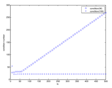
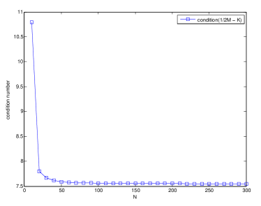
Figure 2: Condition numbers for the matrices $\mathrm{W}_{h}$, $\mathrm{V}_{h}\mathrm{W}_{h}$ and ${\textstyle\frac{1}{2}}\mathrm{M}-\mathrm{K}_{h}$. The results are given for the choice $\alpha=5/6$. Results for $\alpha=1$ are almost identical.

Dependence with respect to $\alpha$

It is unclear from the experiments whether there is a much better choice of the parameter $\alpha$, that dictates the mixture of test functions in the method. Let us first show that $\alpha=1/2$ is not feasible. For a test equation (6.4) we compute the errors $\mathrm{E}_{N}^{\lambda}$ and $\mathrm{E}_{N}^{\mathrm{ext}}$ as $N$ increases. The domain is the curve $\Gamma_{1}$ and the exact solution of the Helmholtz equation is (7.2). It is clear from Figure 3 that $\mathrm{E}_{N}^{\lambda}$ is not converging, while $\mathrm{E}_{N}^{\mathrm{ext}}$ converges with the right order. However, inspection of the condition numbers show that they are of the order $10^{20}$. This makes the method highly unstable. Convergence of the potential solution can be explained by the fact that the potential postprocessing is a smoothing operator which, in some way, eliminates high frequency unstable components of the error and only observes approximation properties. In Figure 4, we explore how the condition numbers of $\mathrm{V}_{h}$ blow up as $\alpha\to 1/2$ and stay large (but considerably smaller) beyond this value.

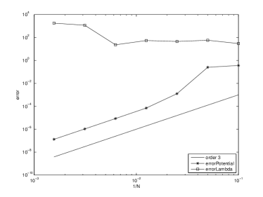
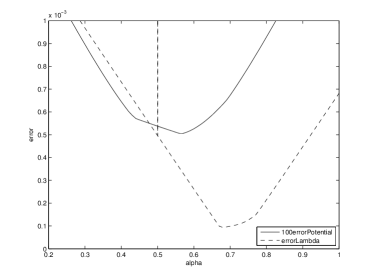
Figure 3: The figure on the left shows history of convergence for the choice $\alpha=1/2$ using a direct single layer potential based method. The method is clearly not converging for the unknown on the boundary, but convergence is restored in the smoothing postprocessing of the potential. The figure on the right shows a history of convergence w.r.t. $\alpha$ for fixed $N$. The peak at $\alpha=1/2$ corresponds to the unstable choice of this parameter.

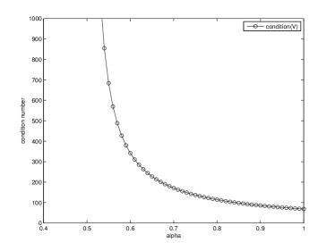
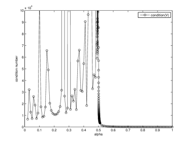
Figure 4: Condition number of the matrix $\mathrm{V}_{h}$ as a function of the parameter $\alpha$. The choice $\alpha=1/2$ equalizes the height of the four Dirac deltas in Figure 1, making the method unstable. Past this threshold, condition numbers are unreasonably high.

8 More complicated problems

8.1 Transmission problems

Consider now the domain $\Omega$ interior to the curve (7.1). In addition to the exterior Helmholtz equation (2.3), we consider an interior equation with a different wave speed

$$\Delta V+(k/c)^{2}V=0\qquad\mbox{in $\Omega$}.$$

An incident wave $U^{\mathrm{inc}}$ is given and two transmission conditions are imposed on $\Gamma$:

$$\gamma^{+}U+\beta_{0}=\gamma^{-}V,\qquad\partial_{\mathbf{n}}^{+}U+\beta_{1}=\kappa\,\partial_{\mathbf{n}}^{-}V.$$

In practical problems $(\beta_{0},\beta_{1}):=(\gamma U^{\mathrm{inc}},\partial_{\mathbf{n}}U^{\mathrm{inc}})$. We choose these transmission data so that the exact solution is the pair given by $U$ in (7.2) and

$$V(\mathbf{z}):=\exp(\imath(k/c)\mathbf{z}\cdot\mathbf{d}),\qquad\mathbf{d}:=({\textstyle\frac{1}{\sqrt{2}}},-{\textstyle\frac{1}{\sqrt{2}}}).$$

We take $k=3$, $c=2/3$, and $\kappa=3/2$. The direct symmetric boundary integral formulation of Costabel and Stephan [9] is used. The unknowns are the Cauchy data for the interior problem, so that the integral representations are

$$U=-\mathrm{S}(k)(\lambda^{-}-\beta_{1})+\mathrm{D}(k)(\varphi^{-}-\beta_{0}),\qquad V=\kappa^{-1}\mathrm{S}({\textstyle\frac{k}{c}})\lambda^{-}-\mathrm{D}({\textstyle\frac{k}{c}})\varphi^{-}.$$

The corresponding system of integral equations is

$$\left[\begin{array}[]{cc}\mathrm{W}(k)+\kappa\,\mathrm{W}(\frac{k}{c})&\mathrm{J}(k)+\mathrm{J}(\frac{k}{c})\\ -\mathrm{K}(k)-\mathrm{K}(\frac{k}{c})&\mathrm{V}(k)+\kappa^{-1}\mathrm{V}(\frac{k}{c})\end{array}\right]\left[\begin{array}[]{c}\varphi^{-}\\ \lambda^{-}\end{array}\right]=\left[\begin{array}[]{cc}\mathrm{W}(k)&\frac{1}{2}\mathrm{I}+\mathrm{J}(k)\\ \frac{1}{2}\mathrm{I}-\mathrm{K}(k)&\mathrm{V}(k)\end{array}\right]\left[\begin{array}[]{c}\beta_{0}\\ \beta_{1}\end{array}\right].$$

We discretize each of the elements in the system of integral equations and in the integral representations using the rules of the discrete Calderón Calculus. Taking $N$ discretization points on the boundary, we compute the exterior error (7.3) and errors on the boundary

$$\mathrm{E}_{N}^{\lambda}:=N\,\max_{j}|\lambda_{j}-\kappa\,\nabla V(\mathbf{m}_{j})\cdot\mathbf{n}_{j}|,\qquad\mathrm{E}_{N}^{\varphi}:=\max_{j}|\phi_{j}-V(\mathbf{m}_{j})|,\quad\mbox{with}\quad\bm{\phi}=\mathrm{Q}\bm{\varphi}.$$

The corresponding errors are plotted in Figure 5.

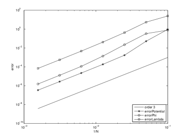
Figure 5: Errors for the transmission problem. On the left, errors for the choice $\alpha=1$. On the right, for $\alpha=5/6$.

8.2 CQ discretization in the time domain

In this final example we show how to combine the fully discrete Calderón Calculus with a Convolution Quadrature routine to produce time-domain discretization of scattering of waves by obstacles. We first explain some general ideas of the CQ method. More details, specifically applied to scattering problems, are given in [2, 21], while the original ideas of multistep-based CQ for hyperbolic problems appear in [22].

Generalities about CQ

We start with a causal approximation of the derivative: if $\kappa>0$, then the operator

$$\partial_{\kappa}u:={\textstyle\frac{1}{\kappa}}({\textstyle\frac{3}{2}}u-u(\cdot-\kappa)+{\textstyle\frac{1}{2}}u(\cdot-2\kappa))$$ (8.1)

is the backward differentiation operator associated to the BDF2 method. The associated transfer function (the Laplace transform of the operator) is

$$s_{\kappa}:={\textstyle\frac{1}{\kappa}}({\textstyle\frac{3}{2}}-2e^{-\kappa s}+{\textstyle\frac{1}{2}}e^{-2\kappa s}).$$ (8.2)

Let now $\mathrm{A}_{h}(s)$ be any of the elements of the discrete Calculus (one of the potentials or one of the operators), with $k=-\imath s$, $s\in\mathbb{C}$ and $\mathrm{Re}\,s>0$. This is the same as saying that we are taking the operators associated to the Laplace resolvent equation $\Delta U-s^{2}U=0$ in $\mathbb{R}^{2}\setminus\Gamma$ (radiation conditions are reduced to imposing $U\in H^{1}(\mathbb{R}^{2}\setminus\Gamma)$, which in practice imposes exponential decay at infinity). After some manipulation in the complex plane, we can write

$$\mathrm{A}_{h}(s_{\kappa})=\sum_{m=0}^{\infty}\mathrm{A}_{\kappa,h}[m]e^{-\kappa ms}.$$

The Convolution Quadrature method is the practical computation of convolutions of the form

$$\mathrm{A}_{h}(\partial_{\kappa})\bm{\psi}=\sum_{m=0}^{\infty}\mathrm{A}_{\kappa,h}[m]\bm{\psi}(\cdot-m\kappa)$$ (8.3)

(compare with (8.1) and (8.2)). The forward convolution form consists of sampling a causal function $\bm{\psi}:\mathbb{R}\to\mathbb{C}^{N}$, denoting $\underline{\bm{\psi}}[n]:=\bm{\psi}(\kappa\,n)$, and then computing

$$\mathrm{A}_{h}(\partial_{\kappa})\underline{\bm{\psi}}[n]:=\sum_{m=0}^{\infty}\mathrm{A}_{\kappa,h}[m]\bm{\psi}[n-m].$$ (8.4)

(Note that we use the same notation, but now $\underline{\bm{\psi}}$ is discrete in time, i.e., it is a sequence of vectors.) The same idea can be used to solve convolution equations (in the same way that (8.1) is the seed of the BDF2 method)

$$\sum_{m=0}^{\infty}\mathrm{A}_{\kappa,h}[m]\bm{\psi}[n-m]=\bm{\xi}[n]\qquad n=0,1,\ldots,$$ (8.5)

where $\bm{\xi}:\mathbb{R}\to\mathbb{C}^{N}$ is a given causal function sampled at the points $\kappa\,n$, or $\bm{\xi}[n]$ are the entries of a sequence of vectors $\underline{\bm{\xi}}$. Note that in (8.4) and (8.5) data ($\bm{\psi}$ and $\bm{\xi}$ respectively) are sampled in the time domain, while the action of the operator is taken using the transfer function. Practical ways of computing these convolutions are explained in [2]. They involve a clever use of FFT, contour integrals, and multiple evaluations of the transfer function $\mathrm{A}_{h}(s)$. In the case of the convolution equation (8.5), repeated inversion of $\mathrm{A}_{\kappa,h}[0]=\mathrm{A}_{h}(s_{0})=\mathrm{A}_{h}({\textstyle\frac{3}{2}}{\textstyle\frac{1}{\kappa}})$ is also required.

A scattering problem

In this first example, we use the time domain version of (6.3) and (6.9). The normal derivative of an incident plane wave $U^{\mathrm{inc}}(t,\mathbf{x})$ is sampled at the observation points at all times

$$\bm{\beta}_{1}^{\pm}[n]:=-(\nabla U^{\mathrm{inc}}(n\,\kappa,\mathbf{m}_{1}^{\pm})\cdot\mathbf{n}_{1},\ldots,\nabla U^{\mathrm{inc}}(n\,\kappa,\mathbf{m}_{N}^{\pm})\cdot\mathbf{n}_{N})^{\top},\quad n\geq 0.$$

We assume that the discrete function $\bm{\beta}_{1}[n]:=\mathrm{P}^{+}\bm{\beta}_{1}^{+}[n]+\mathrm{P}^{-}\bm{\beta}_{1}^{-}[n]$ is causal: this is true in the reasonable physical situation when the incident wave has not reached any of the obstacles at time zero. We then solve equations looking for causal sequences $\underline{\bm{\varphi}}=(\bm{\varphi}[n])$ and $\underline{\bm{\lambda}}=(\bm{\lambda}[n])$ satisfying

$$\mathrm{M}\bm{\lambda}[n]=\bm{\beta}_{1}[n],\qquad\mathrm{W}_{h}(\partial_{k})\underline{\bm{\varphi}}[n]=-{\textstyle\frac{1}{2}}\mathrm{M}\bm{\lambda}[n]-\mathrm{J}_{h}(\partial_{\kappa})\underline{\bm{\lambda}}[n],\qquad\forall n\geq 0.$$ (8.6)

The potentials are then computed at every time step using the CQ method once again, resulting in sequences

$$U[n]=\mathrm{S}_{h}(\partial_{\kappa})\underline{\bm{\lambda}}[n]-\mathrm{D}_{h}(\partial_{\kappa})\underline{\bm{\varphi}}[n].$$ (8.7)

Note that this is a fully discrete method for the scattering of a sound-hard obstacle by a transient incident wave. Note also that the sequence of functions (8.7) are a classical solution of the BDF2-discretized wave equation [22]:

$$\partial_{\kappa}^{2}U[n]-\Delta U[n]=0\qquad\mbox{in $\mathbb{R}^{2}\setminus\Gamma$}\qquad\forall n.$$

To test the method, we change some signs so that we end up solving an interior boundary value problem, namely, we solve $\mathrm{W}_{h}(\partial_{\kappa})\underline{\bm{\varphi}}=\frac{1}{2}\mathrm{M}\underline{\bm{\lambda}}-\mathrm{J}_{h}(\partial_{\kappa})\underline{\bm{\lambda}}$, instead of the second equation in (8.6). The potential solution (8.7) is then an approximation of $-U^{\mathrm{inc}}(n\,\kappa,\cdot)$ in $\Omega_{-}$.

For the experiments we take the boundary of the domain parametrized with

$${\textstyle\frac{1}{10\sqrt{2}}}(4\,(1+\cos^{2}(2\pi t))\cos(2\pi t),5\,(1+\sin^{2}(2\pi t))\sin(2\pi t))\left(\begin{array}[]{cc}1&-1\\ 1&1\end{array}\right),$$

the incident wave given by

$$U^{\mathrm{inc}}(t,\mathbf{z}):=\rho(t\!-\!R\!+\!\mathbf{z}\cdot\mathbf{d}),\quad R=1.2,\quad\mathbf{d}:=(-{\textstyle\frac{1}{\sqrt{2}}},-{\textstyle\frac{1}{\sqrt{2}}}),\quad\rho(t):=\sin^{3}(3\,t)\chi_{t\geq 0},$$

$N$ discretization points on the curve, and $M$ time steps of length $T/M$, where $T=5$. Finally we compute errors

$$\mathrm{E}_{N,M}^{\mathrm{int}} := |U[M](\mathbf{z}_{\circ})+U^{\mathrm{inc}}(T,\mathbf{z}_{\circ})|,\qquad\mathbf{z}_{\circ}=(0.2,0.2),$$

$$\mathrm{E}_{N,M}^{\varphi} := \max_{j}|\phi_{j}[M]+U^{\mathrm{inc}}(T,\mathbf{m}_{j})|,\qquad\bm{\phi}[M]=\mathrm{Q}\bm{\varphi}[M].$$

The values of $N$ and $M$ are chosen so that $\mathcal{O}(N^{-3})=\mathcal{O}(M^{-2})$: for $j=10,\ldots,19$, we define

$$N_{j}=\lfloor 20\,(1.2)^{j}\rfloor,\qquad M_{j}:=\lfloor N^{3/2}\,20^{-1/2}\rfloor,\qquad N_{j}^{3}\approx 20M_{j}^{2},\qquad N_{j+1}/N_{j}\approx 1.2.$$

The results are reported in Table 11. Experimental convergence rates are shown to confirm that the errors in $\mathcal{O}(N^{-3})$.

$N$	$M$	$\mathrm{E}_{N,M}^{\mathrm{ext}}$	e.c.r	$\mathrm{E}_{N,M}^{\varphi}$	e.c.r
123	305	7.1971$E(-002)$		1.3079$E(-001)$
148	402	4.2559$E(-002)$	2.8816	7.6194$E(-002)$	2.9634
178	531	2.4632$E(-002)$	2.9994	4.3811$E(-002)$	3.0353
213	695	1.4327$E(-002)$	2.9723	2.5594$E(-002)$	2.9482
256	915	8.2648$E(-003)$	3.0173	1.4754$E(-002)$	3.0211
308	1208	4.7404$E(-003)$	3.0489	8.4560$E(-003)$	3.0532
369	1584	2.7533$E(-003)$	2.9801	4.9135$E(-003)$	2.9776
443	2084	1.5894$E(-003)$	3.0135	2.8368$E(-003)$	3.0129
532	2743	9.1716$E(-004)$	3.0157	1.6368$E(-003)$	3.0162
638	3603	5.3072$E(-005)$	3.0005	9.4818$E(-004)$	2.9946

Table 11: Errors $\mathrm{E}_{N,M}^{\mathrm{int}}$ and $\mathrm{E}_{N,M}^{\varphi}$ for an interior problem in the time domain.

A final experiment

To illustrate the capabilities of the time-domain discretization, we choose a kite-shaped sound-hard obstacle, hit by a short plane incident wave, and we plot several snapshots of the total wave field (incident plus computed wave). Results are shown in Figure 6.

$t=2.8560$	$t=5.2560$
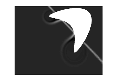
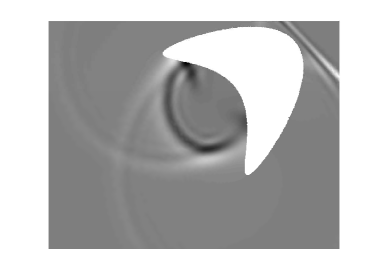
$t=6.6960$	$t=7.6560$
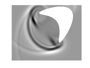
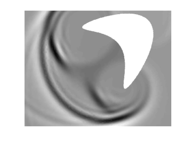
$t=8.3760$	$t=9.0960$

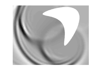
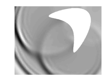
Figure 6: Six snapshots of the scattering of a plane wave by a kite-shaped sound-hard obstacle. The profile of the wave can be oberserved in the first two images, as it travels to the right and to the top. Discretization has been carried out with the order three Calderón Calculus and a BDF2–based Convolution Quadrature routine.

References

- [1] K. Atkinson. The numerical solution of integral equations of the second kind, volume 4 of Cambridge Monographs on Applied and Computational Mathematics. Cambridge University Press, Cambridge, 1997.
- [2] L. Banjai and M. Schanz. Wave propagation problems treated with Convolution Quadrature and BEM. In Fast Boundary Element Methods in Engineering and Industrial Applications, pages 145–184. Lecture Notes in Applied and Computational Mechanics, Volume 63, 2012.
- [3] O. Bruno, V. Domínguez, and F. Sayas. Convergence analysis of a high-order Nyström integral-equation method for surface scattering problems. Numer. Math. To appear.
- [4] O. P. Bruno and L. A. Kunyansky. A fast, high-order algorithm for the solution of surface scattering problems: basic implementation, tests, and applications. J. Comput. Phys., 169(1):80–110, 2001.
- [5] R. Celorrio, V. Domínguez, and F. J. Sayas. Periodic Dirac delta distributions in the boundary element method. Adv. Comput. Math., 17(3):211–236, 2002.
- [6] R. Celorrio and F.-J. Sayas. The Euler-Maclaurin formula in presence of a logarithmic singularity. BIT, 39(4):780–785, 1999.
- [7] G. A. Chandler and I. H. Sloan. Spline qualocation methods for boundary integral equations. Numer. Math., 58(5):537–567, 1990.
- [8] D. Colton and R. Kress. Inverse acoustic and electromagnetic scattering theory, volume 93 of Applied Mathematical Sciences. Springer-Verlag, Berlin, second edition, 1998.
- [9] M. Costabel and E. Stephan. A direct boundary integral equation method for transmission problems. J. Math. Anal. Appl., 106(2):367–413, 1985.
- [10] M. Crouzeix and F.-J. Sayas. Asymptotic expansions of the error of spline Galerkin boundary element methods. Numer. Math., 78(4):523–547, 1998.
- [11] V. Domínguez, S. L. Lu, and F.-J. Sayas. Fully discrete Calderón Calculus for the two dimensional Helmholtz equation. Int. J. Numer. Anal. Model. (in revision).
- [12] V. Domínguez, S. L. Lu, and F.-J. Sayas. A Nyström method for the two dimensional hypersingular operator for the Helmholtz equation. Submitted.
- [13] V. Domínguez, M.-L. Rapún, and F.-J. Sayas. Dirac delta methods for Helmholtz transmission problems. Adv. Comput. Math., 28(2):119–139, 2008.
- [14] C. Epstein, L. Greengard, and A. Klöckner. On the convergence of local expansions of layer potentials. arXiv:1212.3868, 2012.
- [15] I. G. Graham and I. Sloan. Fully discrete spectral boundary integral methods for Helmholtz problems on smooth closed surfaces in . Numer. Math., 92(2):289–323, 2002.
- [16] S. Hao, A. H. Barnett, P. G. Martinsson, and P. Young. High-order accurate Nyström discretization of integral equations with weakly singular kernels on smooth curves in the plane. arXiv:1112.6262, 2011.
- [17] G. C. Hsiao, P. Kopp, and W. L. Wendland. A Galerkin collocation method for some integral equations of the first kind. Computing, 25(2):89–130, 1980.
- [18] A. Klöckner, A. Barnett, L. Greengard, and M. O’Neil. Quadrature by expansion: A new method for the evaluation of layer potentials. arXiv:1207.4461, 2012.
- [19] R. Kress. Linear integral equations, volume 82 of Applied Mathematical Sciences. Springer-Verlag, New York, second edition, 1999.
- [20] R. Kussmaul. Ein numerisches Verfahren zur Lösung des Neumannschen Neumannschen Aussenraumproblems für die Helmholtzsche Schwingungsgleichung. Computing (Arch. Elektron. Rechnen), 4:246–273, 1969.
- [21] A. R. Laliena and F.-J. Sayas. Theoretical aspects of the application of convolution quadrature to scattering of acoustic waves. Numer. Math., 112(4):637–678, 2009.
- [22] C. Lubich. On the multistep time discretization of linear initial-boundary value problems and their boundary integral equations. Numer. Math., 67(3):365–389, 1994.
- [23] E. Martensen. Über eine Methode zum räumlichen Neumannschen Problem mit einer Anwendung für torusartige Berandungen. Acta Math., 109:75–135, 1963.
- [24] E. Nyström. Über Die Praktische Auflösung von Integralgleichungen mit Anwendungen auf Randwertaufgaben. Acta Math., 54(1):185–204, 1930.
- [25] J. Saranen and L. Schroderus. Quadrature methods for strongly elliptic equations of negative order on smooth closed curves. SIAM J. Numer. Anal., 30(6):1769–1795, 1993.
- [26] I. H. Sloan. Qualocation. J. Comput. Appl. Math., 125(1-2):461–478, 2000. Numerical analysis 2000, Vol. VI, Ordinary differential equations and integral equations.
- [27] L. Wienert. Die numerische Approximation von Randintegraloperatoren für die Helmholtzgleichung im . PhD thesis, University of Göttingen, 1990.