Linear stability analysis of fluid flow between two parallel porous stationary plates with small suction and injection

Abstract

In this work, the linear stability of the viscous incompressible fluid flow between two parallel horizontal porous stationary plates with the assumption that there is a small constant suction at upper plate and a small constant injection at the lower plate is studied.The Navier-Stokes and continuous equations are reduced to an equation modified by the suction Reynolds number, which we call modified Orr-Sommerfeld equation. This equation is rewritten as an eigenvalue problem and is solved numerically using Matlab (Windows Version). The effect of small suction Reynolds number on the linear stability fluid flow is discussed.

Institut de Mathématiques et de Sciences Physiques, BP: 613 Porto Novo, Bénin Keywords: Porous parallel plates, linear stability, small suction Reynolds number, modified Orr-Sommerfeld equation.

1 Introduction

The flow through porous boundaries is of great importance both in technological as well as biophysical flows. Examples of this are found in soil mechanics, the aviation industry, transpiration cooling, food preservation, cosmetic industry, blood flow and artificial dialysis. A large number of theoretical investigations dealing with steady incompressible laminar flow with either injection or suction at the boundaries ([1] -[2]) have appeared during the last few decades. Several authors [3] have studied the steady laminar flow of an incompressible viscous fluid in a two- dimensional channel with parallel porous walls. Rioual and al. $(1996)$ studied the power balance of a flat plate used as an airplane wing and found that there is an optimum speed of suction that reduces drag and weaken energy consumption. Recent experimental studies show that suction damps growth of disturbances induced by free stream turbulence and transition is delayed/prevented (Fransson and Alfredsson $2003$). Aspiration may also be used as a tool to induce transition, instead of the delay, if for example the wall material chosen is not able to provide continuous suction (MacManus and Eaton, $2000$) or if it is applied non-uniformly (Roberts and Floryan, $2001$) [4].

In this work, the flow of the incompressible viscous fluid between two parallel horizontal stationary porous plates with the assumption that there is constant small suction at upper plate and a constant small injection at the lower plate is considered. Speeds suction and injection are assumed uniform and same standard $V^{*}_{\omega}$ (see figure (1)) below [3]. The objective is to study the effect of number $R_{e\omega}$ of extradvective term introduced in an Orr-Sommerfeld equation by small suction velocity on the stability of the fluid flow. Such attempt has been made earlier by E. Niklas Davidsson and L. Hakan Gustavsson the $2000s$ ( [1] and [4]) the case of the boundary layers (a flat plate-law) with uniform wall suction by normalizing all the components of the velocity with the free stream velocity $U^{*}$. Before E. Niklas Davidsson and al. ; V. M. Soundalgekar, V. G. Divekar and al. ($1968-1972$) studied the flow quilt with suction at the stationary plate and laminar slip-flow through uniform circular pipe with small suction ( [5]-[6]). All these studies confirm the stabilizing effect of small wall suction on a flow.

The paper is organized as follows. In the second section the modified Orr-Sommerfeld equation governing the stability analysis in the Poiseuille two parallel horizontal porous stationary plates flow will be checked. In the third section an analysis of the small suction Reynolds number $R_{e\omega}$ stabilizing effect will be investigated. The conclusions will be presented in the final section.

2 modified Orr-Sommerfeld equation

The motion of a fluid is governed by the conservation laws, such as conservation of mass and momentum. The momentum of the fluid changes due to the forces acting upon it, and is governed by Newton’s second law of motion. Fluids at low velocity compared to the speed of sound can be considered incompressible, i.e. the density of the fluid is constant. The stress acting on a fluid element may be linearly proportional to the local pressure and velocity gradient. For an incompressible, newtonian fluid the momentum and conservation equations yield

$$\frac{\partial{\tilde{u}_{i}^{*}}}{\partial{\tilde{t}^{*}}}+\tilde{u}_{j}^{*}\frac{\partial{\tilde{u}_{i}^{*}}}{\partial{\tilde{x}_{j}^{*}}} = -\frac{1}{\rho}\frac{\partial{\tilde{p}}^{*}}{\partial{\tilde{x}_{i}^{*}}}+{\nu}\frac{\partial^{2}{\tilde{u}_{i}^{*}}}{{\partial{\tilde{x}_{j}^{*}}}^{2}}$$ (1)

$$\frac{\partial{\tilde{u}_{i}^{*}}}{\partial{\tilde{x}_{i}^{*}}} = 0$$ (2)

when written by Einsteins’ summation convention. These are the Navier-Stokes (N$-$S) equations. Here $\tilde{x}^{*}_{i}$ and $\tilde{u}^{*}_{i}$ are the $i^{ieme}$ component of the space and velocity vectors, as commonly in the literature denoted $(\tilde{x}^{*},\tilde{y}^{*},\tilde{z}^{*})$ and $(\tilde{u}^{*},\tilde{v}^{*},\tilde{w}^{*})$ in the streamwise, wall-normal and spanwise directions, respectively. Also, $\tilde{P}^{*}$ is the pressure, $\rho$ is the density and $\nu$ is the kinematical viscosity of the fluid.

We Considered the viscous and incompressible fluid flow between two parallel horizontal stationary porous flat plates under a constant gradient of pressure with small wall suction and injection in the figure (1) below [3].

Figure 1: Poiseuille porous parallel flat plates flow.

The coordinates (streamwise $x$, the wall-normal $y$ and spanwise $z$) are scaled with the length scale $h^{*}$ ( distance between the two walls). The streamwise and spanwise velocities $u$ and $w$, respectively, are scaled with the streamwise free stream velocity $U^{*}$ while the wall-normal velocity $v$ is scaled with the characteristic velocity of suction and injection $V_{\omega}^{*}$. The pressure $p$ is scaled with $\rho U^{*2}$ and the time $t$ with $\frac{h^{*}}{U^{*}}$. The Reynolds’ numbers used here are defined as $R_{e}=\frac{U^{*}h^{*}}{\nu}$ and suction Reynolds’ number $R_{e\omega}=\frac{V_{\omega}^{*}h^{*}}{\nu}$ where $\nu$ is kinematic viscosity.
We want to study the linear stability of a high Reynolds $R_{e}$ and small suction Renynolds $R_{e\omega}$ ($0\leq R_{e\omega}\leq 1$) numbers flow. The non-dimensional Navier-Stokes and continuous (Conservation of mass) linearized equations (1) and (2) where the variables are normalized as above take the following forms

$$\frac{\partial{{\tilde{u}}}}{\partial{{\tilde{t}}}}+{\tilde{u}}\frac{\partial{\tilde{u}}}{\partial{\tilde{x}}}+\frac{R_{e\omega}}{R_{e}}{\tilde{v}}\frac{\partial{\tilde{u}}}{\partial{\tilde{y}}}+{\tilde{w}}\frac{\partial{\tilde{u}}}{\partial{\tilde{z}}} = -\frac{\partial{\tilde{p}}}{\partial{\tilde{x}}}+\frac{1}{R_{e}}{\bigtriangledown}^{2}{\tilde{u}},$$ (3)

$$\frac{\partial{{\tilde{v}}}}{\partial{{\tilde{t}}}}+{\tilde{u}}\frac{\partial{\tilde{v}}}{\partial{\tilde{x}}}+\frac{R_{e\omega}}{R_{e}}{\tilde{v}}\frac{\partial{\tilde{v}}}{\partial{\tilde{y}}}+{\tilde{w}}\frac{\partial{\tilde{v}}}{\partial{\tilde{z}}} = -\frac{R_{e}}{R_{e\omega}}\frac{\partial{\tilde{p}}}{\partial{\tilde{y}}}+\frac{1}{R_{e}}{\bigtriangledown}^{2}{\tilde{v}},$$ (4)

$$\frac{\partial{{\tilde{w}}}}{\partial{{\tilde{t}}}}+{\tilde{u}}\frac{\partial{\tilde{w}}}{\partial{\tilde{x}}}+\frac{R_{e\omega}}{R_{e}}{\tilde{v}}\frac{\partial{\tilde{w}}}{\partial{\tilde{y}}}+{\tilde{w}}\frac{\partial{\tilde{w}}}{\partial{\tilde{z}}} = -\frac{\partial{\tilde{p}}}{\partial{\tilde{z}}}+\frac{1}{R_{e}}{\bigtriangledown}^{2}{\tilde{w}}.$$ (5)

$$\frac{\partial{\tilde{u}}}{\partial{\tilde{x}}}+\frac{R_{e\omega}}{R_{e}}\frac{\partial{\tilde{v}}}{\partial{\tilde{y}}}+\frac{\partial{\tilde{w}}}{\partial{\tilde{z}}} = 0,$$ (6)

For stability analysis, the flow is decomposed into the mean flow and the disturbance according to

$$\tilde{u}_{i}(r,t) = U_{i}(r)+u_{i}(r,t),$$ (7)

$$\tilde{p}(r,t) = P(r)+p(r,t).$$ (8)

We take the dimensional base flow for small suction and injection (see [3])

$$U(y) = U^{*}(1-\frac{y^{2}}{h^{*2}})$$ (9)

$$V = V^{*}_{\omega}$$ (10)

$$W = 0.$$ (11)

By scaling these velocities as above, we obtain with $h^{*}=\pm 1$ the no-dimensional base flow

$$U(y) = (1-y^{2})$$ (12)

$$V = 1$$ (13)

$$W = 0.$$ (14)

To obtain the stability equations for the spatial evolution of three-dimensional, we take the dependent on time disturbances

$$(u(x,y,z,t);v(x,y,z,t);w(x,y,z,t);p(x,y,z,t));$$ (15)

which are scaled in the same way as above.
By using continuity, the pressure terms can be eliminated from Navier-Stokes equations. For such a mean profile (base flow), the divergence of Navier-Stokes equations and continuity gives

$${\bigtriangledown}^{2}{p} = -2\frac{R_{e\omega}}{R_{e}}\frac{\partial{U}}{\partial{y}}\frac{\partial{v}}{\partial{x}}.$$ (16)

The equations (4) and (16) after linearization give

$$\frac{\partial{}}{\partial{t}}{\bigtriangledown}^{2}{v}+{U}\frac{\partial{}}{\partial{x}}{\bigtriangledown}^{2}{v}+\frac{R_{e\omega}}{R_{e}}\frac{\partial{}}{\partial{y}}{\bigtriangledown}^{2}{v}-\frac{d^{2}U}{{dy}^{2}}\frac{\partial{v}}{\partial{x}} = \frac{1}{R_{e}}{\bigtriangledown}^{4}{v}.$$ (17)

The disturbances are taken to be periodic in the streamwise, spanwise directions and time, which allow us to assume solutions of the form

$$f(x,y,z,t) = \hat{f}(y)e^{i(\alpha x+\beta z-\omega t)};$$ (18)

where $f$ represents either one of the disturbances $u$, $v$, $w$ or $p$ and $\hat{f}$ the amplitude function, $k$, $\alpha=k_{x}=k\cos{\theta}$ and $\beta=k_{y}=k\sin{\theta}$ are the wave numbers, $\omega=\alpha c$ the pulsation of the wave. With $i^{2}=-1$, $\theta=(\vec{k_{x}},\vec{k})$, $c=c_{r}+ic_{i}$ wave velocity which is taken to be complex, $\alpha$ and $\beta$ are real because of temporel stability analysis considered.
Then with the equation (18), the equation (17) becomes

$$i\alpha\left[\left(U-c\right)\left(D^{2}-{k}^{2}\right)-{U^{\prime\prime}}\right]\hat{v} = -\frac{R_{e\omega}}{R_{e}}D\left(D^{2}-{k}^{2}\right)\hat{v}$$

$$+\frac{1}{R_{e}}\left(D^{2}-{k}^{2}\right)^{2}\hat{v};$$ (19)

where $D=\frac{d}{dy}$ ; with boundary conditions for all $(x,\pm 1,z,t)$

$$\hat{v}(\pm 1) = 1$$

$$\hat{v}^{\prime}(\pm 1) = 0.$$ (20)

Taking

$$v_{p}(x,y,z,t) = \hat{v}(y)e^{i(\alpha x+\beta z-\omega t)}-1,$$ (21)

the equation (19) and the boundary conditions take the forms

$$\left[\left(U-{\bf{i\alpha^{-1}\frac{R_{e\omega}}{R_{e}}D}}\right)\left(D^{2}-k^{2}\right)-U^{\prime\prime}-i\alpha^{-1}\frac{1}{R_{e}}(D^{2}-k^{2})^{2}\right]\hat{v}_{p}=$$

$$c\left(D^{2}-k^{2}\right)\hat{v}_{p},$$ (22)

$$\hat{v}_{p}(\pm 1) = 0$$

$$\hat{v}_{p}^{\prime}(\pm 1) = 0.$$ (23)

The equation (22) is a flow equation modified by suction Reynolds number ${R_{e\omega}}$ (or the speed of suction and injection), which we call modified Orr-Sommerfeld equation, rewritten as an eigenvalue problem.

3 Stability analysis

We consider our three-dimensional disturbances. We use a temporal stability analysis as mentioned above. With $c$ complex as we have defined above, when $c_{i}<0$ we have stability, $c_{i}=0$ we have neutral stability and else we have instability. We employ Matlab (Windows Version) in all our numerical computations to find the eigenvalues. The Poiseuille parallel horizontal stationary porous plates flow with the basic profile

$${\bf{U}}=\left(1-y^{2},1,0\right)$$ (24)

for $R_{e\omega}$ small ( i.e. small suction) is considered (see [3]). The eigenvalue problem (22) is solved numerically with a suitable boundary conditions. The solutions are found in a layer bounded at $y=\pm 1$ with ${\bf{U}}(\pm 1)=(0,1,0)$. The results of calculations are presented in the figures below. We present the figures related to the eigenvalue problem (22).

For all these figures the black, red, green and blue colors are respectively, for $R_{e\omega}=0$, $R_{e\omega}=0.5$, $R_{e\omega}=0.75,$ $R_{e\omega}=1$ and the yellow color is for $c_{i}=0$.

In each group of four figures, the first one is Figure a), the second is Figure b), the third is Figure c) and the fourth is Figure d).

For a fixed $k=1$, we get figure (3) of $c_{i}$ vs. $R_{e}$ for sequential values of $\theta$. figure $a$) for $\theta=0$, figure $b)$ for $\theta=0.1\pi$, figure $c)$ for $\theta=0.2\pi$ and figure $d)$ for $\theta=0.3\pi$.

For a fixed $k=1.02$, we get figure (4) of $ci$ vs. $R_{e}$ for sequential values of $\theta$. figure $a$) for $\theta=0$, figure $b)$ for $\theta=0.1\pi$, figure $c)$ for $\theta=0.2\pi$ and figure $d)$ for $\theta=0.3\pi$.

For a fixed $k=2$, we get figure (5) of $ci$ vs. $R_{e}$ for sequential values of $\theta$. figure $a$) for $\theta=0$, figure $b)$ for $\theta=0.1\pi$, figure $c)$ for $\theta=0.2\pi$ and figure $d)$ for $\theta=0.3\pi$.

For a fixed $k=3$, we get figure (6) of $ci$ vs. $R_{e}$ for sequential values of $\theta$. figure $a$) for $\theta=0$, figure $b)$ for $\theta=0.1\pi$, figure $c)$ for $\theta=0.2\pi$ and figure $d)$ for $\theta=0.3\pi$.

Through the Figures (3 and 4), it is easy to see that the stability increases when $R_{e\omega}$ increases for all $\theta$ because, for any familly of curves of these figures the slope fall when the suction Reynolds’ number increases. The Reynolds’ critical number $R_{ec}$ for which we have the transition becomes important when $R_{e\omega}$ increases (see tabular (2)) which confirms that the wall small suction or injection have a stabilizing effect on the viscous incompressible flow. Because of $R_{e\omega}$ influences, we said that to normalize with the characteristic velocity of suction is necessary for a perfect command of the field of stability. In particular for ($R_{e\omega}=0,k=1.02$, without suction, figure (4) black curve ($a$) ) we find $R_{ec}=5772$ which corresponds exactly to the critical value given by classical linear theory for a plane-Poiseuille flow without suction or injection.

For $R_{e\omega}=1$, the equation (22) is identicaly for the equation $(2.28)$ found by E. Niklas Davidsson and L. Hakan Gustavsson in [1]. For this value of $R_{e\omega}$ in the cases of figures (3 and 4) the field of stability is more greater than the other small suction Reynolds number for all $\theta$.

Note that for great $k$ the case of the Figures (5) and (6) there is stability without transition for all value of $\theta$ and $R_{e\omega}$ but when the small suction $R_{e\omega}$ increases the field of stability decreases. We can also say that $k$ influences the stability of the flow i.e. the growth of the wave number induces also the stability of the flow. We therefore conclude that in two parallel horizontal stationary porous plates viscous and incompressible fluid flow, with small suction and small injection, the small suction Reynolds number stabilize the flow for small wave number but the high wave number effect is important than small suction Reynolds’ number on the fluid flow stability.

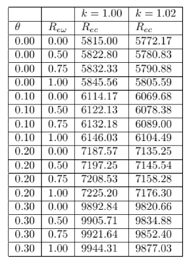
Figure 2: Tabular for critical Reynolds numbers

figures

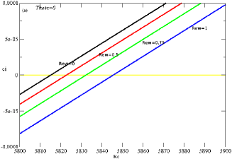
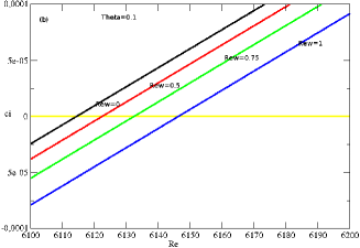
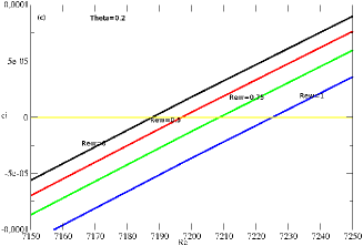
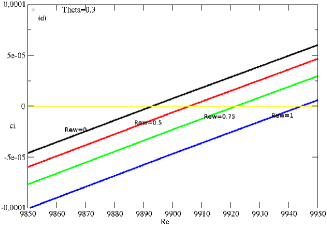
Figure 3: Growth rate $c_{i}$ vs. Reynolds’ number for $k=1$.

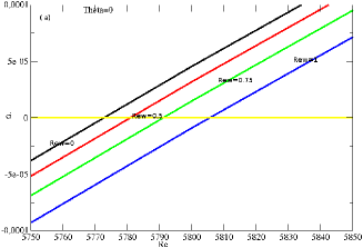
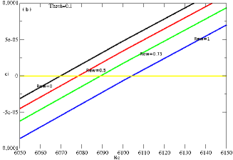
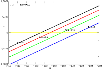
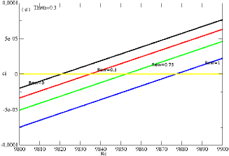
Figure 4: Growth rate $c_{i}$ vs. Reynolds’ number for $k=1.02$.

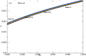
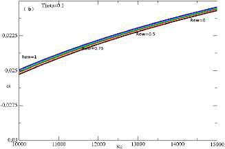
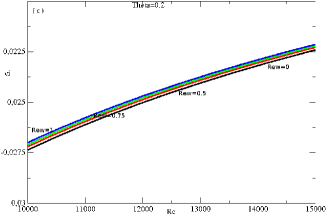
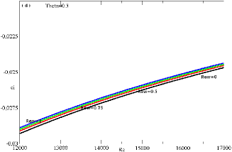
Figure 5: Growth rate $c_{i}$ vs. Reynolds’ number for $k=2$.

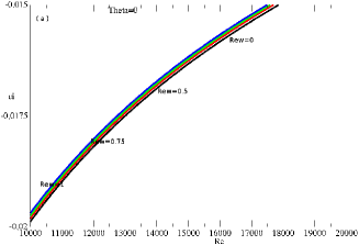
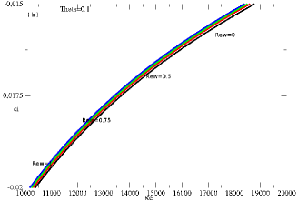
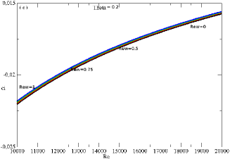
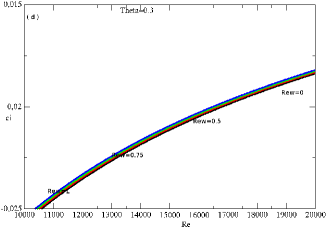
Figure 6: Growth rate $c_{i}$ vs. Reynolds’ number for $k=3$.

4 Conclusion

In this paper, we have investigated the effect of small suction Reynolds number on the stability of the fluid flow between two parallel horizontal stationary porous plates . We have shown that the instability of the perturbed flow is governed by a remarkably equation named modified Orr-Sommerfeld equation. We find also that the normalization of the wall-normal velocity with characteristic small suction (or small injection) velocity is important for a perfect command of fluid flow stability analysis. We noticed that for $k=1.02$ and $R_{e\omega}=0$ we find $R_{ec}=5772$ which corresponds exactly to the critical value given by classical linear theory for a plane-Poiseuille flow without suction or injection. We noticed also that the high wave number stabilize more than the small suction Reynolds number.

References

- [1] E. Niklas Davidsson and L. Hakan Gustavsson, Elementary solutions for streaky structures in boundary layers with and without suction. Accepted for publication in Fluid Dynamics Research.
- [2] O. Levin, E.N. Davidsson and D.S. Henningson, Transition thresholds in the asymptotic suction boundary layer. Physics of Fluids , , .
- [3] Frank M. White, Book-VISCOUS FLUID FLOW, Second Edition.
- [4] E. Niklas Davidsson, Thesis of Luleå University of Technology Department of Applied Physics and Mechanical Engineering Division of Fluid Mechanics - Stability and Transition in the Suction Boundary Layer and other Shear Flows.
- [5] J. L. BANSAL and P. L. Bhatnagar -Laminar flow through a uniform circular pipe with small suction.
- [6] V. M. Soundalgekar and V. G. Divekar - Laminar slip- flow through a uniform circular pipe with small suction. Publications de l’Institut de Mathématique Nouvelle série, tome