Continuation of localised coherent structures in nonlocal neural field equations

Abstract

We study localised activity patterns in neural field equations posed on the Euclidean plane; such models are commonly used to describe the coarse-grained activity of large ensembles of cortical neurons in a spatially continuous way. We employ matrix-free Newton-Krylov solvers and perform numerical continuation of localised patterns directly on the integral form of the equation. This opens up the possibility to study systems whose synaptic kernel does not lead to an equivalent PDE formulation. We present a numerical bifurcation study of localised states and show that the proposed models support patterns of activity with varying spatial extent through the mechanism of homoclinic snaking. The regular organisation of these patterns is due to spatial interactions at a specific scale associated with the separation of excitation peaks in the chosen connectivity function. The results presented form a basis for the general study of localised cortical activity with inputs and, more specifically, for investigating the localised spread of orientation selective activity that has been observed in the primary visual cortex with local visual input.

1 Introduction

One of the most challenging research questions in neuroscience is understanding the relationship between spatially-structured cortical states and the underlying neural circuitry that supports them. A popular approach for analysing coarse-grained activity of large ensembles of neurons in the cortex is to model cortical space as a continuum. Since the pioneering work of Wilson and Cowan [58, 59] and Amari [1, 2], continuous neural field models have become a popular and effective tool in neuroscience. In such models, the large-scale activity of spatially-extended networks of neurons is described in terms of nonlinear integro-differential equations, whose associated integral kernels represent the spatial distribution of neuronal synaptic connections. The canonical Wilson-Cowan-Amari neural field equation [59, 2]

$$\frac{\partial}{\partial t}u(\mathbf{r},t)=-u(\mathbf{r},t)+\int_{\Omega}w(\mathbf{r},\mathbf{r}^{\prime})S\big{(}u(\mathbf{r}^{\prime},t)\big{)}\text{dm}(\mathbf{r}^{\prime})$$ (1)

describes the evolution of the average membrane voltage potential of a neuronal population $u(\mathbf{r},t)$, at position $\mathbf{r}\in\Omega$ on the cortex and at time $t$. The nonlinear function $S$ represents the neural firing rate, whereas the connectivity function $w(\mathbf{r},\mathbf{r}^{\prime})$ models how a population of neurons at position $\mathbf{r}$ on the cortex interacts with a population at position $\mathbf{r}^{\prime}$. Frequently-used firing rate functions $S$ include the Heaviside step function, piecewise-linear functions or smooth sigmoidal functions. Various choices are also possible for the connectivity function, which is often assumed to be translation invariant (that is, dependent on the Euclidean distance $\|\mathbf{r}-\mathbf{r}^{\prime}\|$) and localised in space. The cortical domain $\Omega$ is usually a subset of $\mathbb{R}^{d}$, with $d=1$ or, in more realistic models, $d=2$. For a recent review on neural fields modeling, we refer to Bressloff [8].

Unlike spiking neural network models, continuous field models have the advantage that analytic techniques for partial differential equations (PDEs) can be adapted to study the formation of patterns and their dependence upon control parameters. Various types of coherent structures have been observed in neural field models, ranging from spatially and temporally periodic patterns to travelling waves and spiral waves [27, 19, 42]. Neural field equations have also successfully been used to model a wide range of neurobiological phenomena such as visual hallucinations [28, 9], mechanisms for short term memory [44] and feature selectivity in the visual cortex [6, 35].

A common strategy to derive analytical and numerical results for the nonlocal Eq. (1) is to assume translation invariance and exploit the freedom in the choice of the connectivity function $w$: if the Fourier Transform of $w$ is a rational function, it is possible to derive a PDE formulation that is equivalent to the integral model [42]. Coherent structures supported by the original model can then be conveniently constructed and analyzed in the PDE framework. Indeed, previous studies have been carried out in cases where the synaptic kernel led to an equivalent PDE formulation [44, 43]. To the best of the author’s knowledge, there has been no attempt to propose efficient path-following methods for general connectivity functions $w$. This paper is motivated by the desire to develop numerical algorithms for Eq. (1) without relying on an equivalent PDE formulation. More precisely, we discuss how to solve Eq. (1) when $\Omega=\mathbb{R}^{2}$, $S$ is a smooth function of sigmoidal type and $w$ has a generic Fourier Transform.

The main tools for our investigation are time simulation and numerical continuation. When a PDE model is available, we use standard techniques for both tasks, in line with what is typically done in several other works in this field [43, 41, 42]. However we show that, when the integral of Eq. (1) can be written as a convolution, it is convenient to employ a fast Fourier transform (FFT) for both time stepping and numerical continuation. Direct numerical simulations of Eq. (1) using FFTs have been performed before on full integral models [32, 23]. In the present paper, we combine FFTs with Newton-Krylov solvers [38, 39], thus opening up the possibility to perform numerical continuation directly on the integral model.

We concentrate our effort on the emergence and bifurcation structure of stationary localised patterns in planar neural field models of the form Eq. (1). Indeed, this type of solution is of great interest in models of prefrontal cortex, where localised states are believed to characterise working memory [18, 33]. Recently, localised regions of activity have been observed in the cat primary visual cortex [17] when the animal is presented with localised-oriented input. Moreover, some reported drug-induced visual hallucinations have also been found to be spatially localised [54] indicating the existence of spatially localised regions of activity in the human primary visual cortex.

Localised states have been observed in a wide variety of nonlinear media [40]. The bifurcation structure of localised solutions has been studied extensively in the Swift–Hohenberg equation posed on the real line [25, 60, 11, 12, 16] and on the plane [5, 46, 47, 3, 52, 51, 45]. In this context, a well-known mechanism for the formation of localised states is homoclinic snaking: solutions with one or more bumps at the core emerge from the trivial homogeneous state and undergo a series of fold bifurcations, giving rise to a hierarchy of states with an increasing number of bumps. This scenario seems to be a common footprint of localised patterns, extending far beyond the prototypical Swift–Hohenberg equation [53, 36] and to have also been found in nonlocal equations such as neural fields [44, 21, 43, 29].

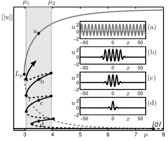
Fig. 1: Bifurcation diagram showing snaking behavior for the 1D neural field equation using Eqs. (2)–(3) with $\theta=3.5$ and $b=0.4$, where stable (unstable) branch segments are represented with solid (dashed) lines. Two branches of solutions bifurcate from the trivial states at a Reversible Hopf bifurcation $R\!H$, namely a branch of periodic solutions (grey) and a branch of localised solutions (black). The periodic branch is stable above the fold $L_{\textrm{p}}$. The localised branch undergoes a series of fold bifurcations giving rise to stable branch segments with increasing numbers of bumps. Several examples of solutions are shown in the insets (a)–(d). Stable localised states exist for $\mu\in[\mu_{1},\mu_{2}]$.

An example of homoclinic snaking is given in Fig. 1, where we show a bifurcation diagram for the integral model (1) posed on the real line with

$$w(x,x^{\prime}):=w(|x-x^{\prime}|) =e^{-b|x-x^{\prime}|}(b\sin|x-x^{\prime}|+\cos(x-x^{\prime})),$$ (2)

$$S(u) =\frac{1}{1+e^{-\mu u+\theta}}-\frac{1}{1+e^{\theta}},$$ (3)

where $b$ and $\mu$ control the decay of the synaptic kernel and the slope of the sigmoidal firing rate respectively, while $\theta$ is a threshold value. As $\mu$ varies, the trivial steady state $u=0$ bifurcates at a subcritical Reversible Hopf bifurcation, from which a branch of periodic solutions and a branch of localised states originate. Beyond the fold $L_{\textrm{p}}$ on the periodic branch, a stable periodic state, shown in the inset (a), coexists with the trivial state. The branch of localised states features solutions with an odd number of bumps and snakes for $\mu\in[\mu_{1},\mu_{2}]$; in this interval, localised solutions with different spatial extent coexist and are stable (see insets (b)–(d)). We note the existence of a counterpart even-numbered-bump solution branch along with so-called ladder branches connecting the odd and even branches (not shown). For the same connectivity function used here, snaking has been shown to occur in terms of the parameter $b$ [44]. Elsewhere, Elvin et al.[26] used the Hamiltonian structure of the steady states of the model (1) with (2)–(3) and developed numerical techniques to find homoclinic orbits of the system. Snaking has also been shown to occur with a Mexican-hat connectivity function [21] and for a wizard-hat connectivity function [29]. In the latter study, normal form theory for a Reversible Hopf bifurcation was applied to prove the existence of localised solutions and a comprehensive parameter study was carried out with numerical continuation in terms of two parameters controlling the nonlinearity and a third controlling the shape of the connectivity function.

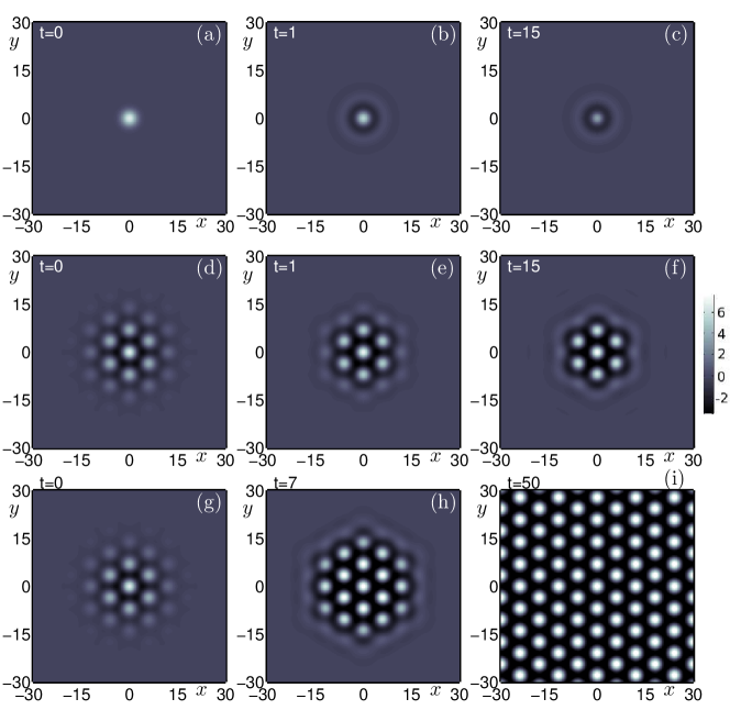
Fig. 2: Time simulations of the integral model (1) posed on the plane, with connectivity function given by Eq. (4) and firing rate function given by Eq. (2); in all simulations $\theta=5.6$, $b=0.4$. (a)–(c): Convergence of a small bump of activity, given by Eq. (20), to a spot solution with $\mu=3.4$; time as indicated in panels. (d)–(f): Convergence of a hexagonal pattern, given by Eq. (21), to a stable $\mathbf{D6}$-symmetric localised state with $\mu=3.2$. (g)–(i) With the same initial condition as (d), divergence away from a localised state to a periodic state with $\mu=3.4$.

For the neural field equation posed on the Euclidean plane, various types of spatially localised two-dimensional states have been found including radially symmetric solutions [55, 57, 44, 43, 32, 10, 30], rings [50, 23], hexagonal patches [43, 30] along with more complex breathing and travelling states [31, 50, 22]. When working in the Euclidean plane, it is still possible to derive an equivalent PDE for suitable choices of the connectivity function $w$ or of its Fourier transform $\widehat{w}$ [43]. Following this approach, normal form theory has recently been applied to prove the existence of localised solution branches in both the Euclidean plane and on the Hyperbolic disk with a wizard-hat connectivity function [30]. When these solutions were path-followed using numerical continuation, it was found that the branches do not undergo snaking-type behaviour. However, for the connectivity (2), snaking was shown to occur for branches of radially-symmetric solutions [43]. Furthermore, the existence of $\mathbf{D6}$-symmetric and $\mathbf{D3}$-symmetric localised states were found at isolated parameter values.

In Fig. 2 we show time simulations of the nonlocal Eq. (1) posed on the plane, with radially-symmetric connectivity function

$$w(\mathbf{r},\mathbf{r}^{\prime}):=w(\|\mathbf{r}-\mathbf{r}^{\prime}\|)=e^{-b\|\mathbf{r}-\mathbf{r}^{\prime}\|}(b\sin\|\mathbf{r}-\mathbf{r}^{\prime}\|+\cos\|\mathbf{r}-\mathbf{r}^{\prime}\|),$$ (4)

and sigmoidal firing rate function given by Eq. (3); various combination of initial conditions and control parameters lead to three different steady states. We note that this models supports localised states, such as the radially-symmetric spot of panel (c) or the hexagonal pattern of panel (f). Furthermore, changes in the slope of the sigmoidal firing rate affect the stability properties of the solutions, leading to other localised states or to domain-covering patterns such as the one in panel (i). In the present paper we will focus on localised planar patterns (with various symmetry properties) that coexist with the trivial state $u=0$ and with fully periodic states, similar to the one shown in Fig. 1 for the 1D case.

A key result of the present paper is that homoclinic snaking occurs in planar neural field models for non-radial patterns and that the choice of the connectivity function has a considerable impact on the snaking structure, as well as on the stability properties and the selection of the localised states. In two spatial dimensions, periodic and localised solution branches bifurcate from the trivial state at a Turing instability (as opposed to a Reversible Hopf in 1D) and snake irregularly, in a similar fashion to what is found for the planar Swift–Hohenberg equation [46].

The outline of the paper is as follows. In Sec. 2, we present the different models that we study, and then, in Sec. 3, we describe the numerical methods that are used to analyze each model. Our homoclinic snaking results of localised states are presented in Sec. 4.

2 Models

In this section, we introduce several neural field models used in the paper: our starting points are the models introduced by Laing et al.[43, 42], in which the cortical space $\Omega$ is assumed to be the Euclidean plane $\mathbb{R}^{2}$.

2.1 Integral model

The first model that we will consider is obtained from Eq. (1) assuming a translation-invariant, radially-symmetric kernel

$$\frac{\partial}{\partial t}u(\mathbf{r},t)=-u(\mathbf{r},t)+\int_{\mathbb{R}^{2}}w(\|\mathbf{r}-\mathbf{r}^{\prime}\|)\;S\big{(}u(\mathbf{r}^{\prime},t)\big{)}\;d\mathbf{r}^{\prime}+g(\mathbf{r})$$ (5)

with sigmoidal firing rate (shown in Fig. 3(a))

$$S(u)=\frac{1}{1+e^{-\mu u+\theta}}-\frac{1}{1+e^{\theta}},\qquad\mu,\theta>0,$$ (6)

radial connectivity function

$$w\left(r\right)=e^{-br}(b\sin r+\cos r),\qquad r=\|\mathbf{r}\|,\quad b>0$$ (7)

and external inhomogeneous input

$$g(\mathbf{r})=G_{0}\exp\Bigg{(}-\frac{\alpha x^{2}+\beta y^{2}}{\sigma^{2}}\Bigg{)},\qquad G_{0},\sigma\in\mathbb{R},\quad\alpha,\beta>0.$$ (8)

In the visual cortex regions of activation have been shown to have a Gaussian spread for radially-symmetric visual inputs [17], hence our choice for the function $g(\mathbf{r})$.

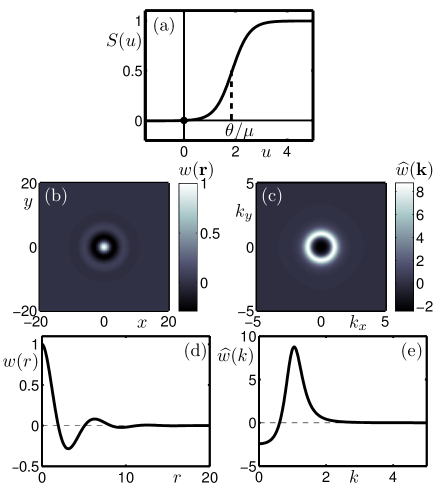
Fig. 3: Firing rate function and connectivity function for the integral model (IM). (a): Sigmoidal nonlinearity given by Eq. (6) plotted here with $\theta=5.6$ and $\mu=3$; in this formulation the effective threshold is $\theta/\mu$ (dashed line). (b): Radially-symmetric connectivity kernel given by Eq. (7) plotted on the Euclidean plane with $b=0.4$. (c): Its Fourier transform plotted on the $(k_{x},k_{y})$-plane. (d): Radial cross section of panel (b). (e): Radial cross section of panel (c).

The connectivity function is plotted in Fig. 3(b) on the Euclidean plane and as a radial cross section in Fig. 3(d). An analytical expression for the Fourier transform of $w$ cannot be obtained; we show the Fourier transform of Eq. (7) as computed numerically in the $\mathbf{k}=(k_{x},k_{y})$-plane in Fig. 3(c) and as a radial cross section in Fig. 3(e), where $k=\|\mathbf{k}\|$. The connectivity function (7) was proposed in models of working memory as a description of synaptic connections in the prefrontal cortex [34, 44]. The connectivity describes local excitation and longer-range connections that alternate between inhibition ($w(r)<0$) and excitation ($w(r)>0$). We argue that this type of connectivity pattern is also relevant to the study of patterns of activity in early visual areas like V1 where there is a characteristic length scale associated with the average orientation hypercolumn width. It has been shown in anatomical studies that the number of lateral connections decay with distance, that the number of excitatory connections peak each hypercolumn width and the number of inhibitory connections peak each half-hypercolumn width [13]. The net effect is alternating bands of inhibition and excitation that decay with distance. This is also consistent with auto-correlations computed for the orientation selectivity map [49] given that connections tend to be reinforced between neurons with similar orientation preference. Henceforth the model (5)–(7) will be referred to as the integral model (IM).

2.2 Fourth-order PDE approximation

In the cases when the Fourier transform of the synaptic kernel is a rational function, it is possible to derive an equivalent PDE formulation of Eq. (5) [42]. For simplicity, we will consider models without an external input $g(\mathbf{r})$. If $\widehat{w}(k)=P(k)/Q(k)$ with $P$ and $Q$ even functions in $k$ where $k=\|\mathbf{k}\|$ for $\mathbf{k}\in\mathbb{R}^{2}$, then the Fourier transform of Eq. (5) gives

$$Q(k)\bigg{[}\frac{\partial}{\partial t}\widehat{u}(\mathbf{k},t)+\widehat{u}(\mathbf{k},t)\bigg{]}=P(k)\widehat{(S\circ u)}(\mathbf{k},t).$$

An inverse Fourier transform of the equation above leads to the desired PDE

$$\mathcal{L}_{Q}\bigg{[}\frac{\partial}{\partial t}u(\mathbf{r},t)+u(\mathbf{r},t)\bigg{]}=\mathcal{L}_{P}S\big{[}u(\mathbf{r},t)\big{]},$$

where $\mathcal{L}_{P}$ and $\mathcal{L}_{Q}$ are linear operators containing spatial derivatives of even order.

Since the Fourier transform of the connectivity function (7) does not have an analytic expression, the integral model does not admit an equivalent PDE. However, we can approximate $w$ with a function whose Fourier transform is rational and then derive an approximate PDE for the integral model. We specify the approximate connectivity function $w_{4}(r)$ through its Hankel Transform

$$w_{4}(r)=\frac{1}{2\pi}\int_{0}^{\infty}s\,\widehat{w_{4}}(s)J_{0}(rs)\;ds,$$

where $\widehat{w_{4}}(k)\approx\widehat{w}(k)$ is given by

$$\widehat{w_{4}}(k)=\frac{A}{B+(k^{2}-M)^{2}}$$ (9)

and the coefficients $A$, $B$, $M$ are determined using a least-squares best fit algorithm (see Sec. 3.4.3 for further details).

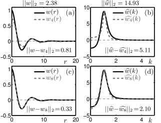
Fig. 4: Comparison of the PDE connectivity functions with $w(r)$ given by Eq. (7) and its Fourier transform $\widehat{w}(r)$ as computed numerically. Panels (a) and (b) show the $4$th-order approximation defined by Eq. (9) in the real and Fourier domains, respectively. Similarly, for the $8$th-order approximation given by Eq. (11) in panels (c) and (d). For reference, we indicate the $L_{2}$-norm of $w$, $w-w_{4}$, $w-w_{8}$ and of their Fourier transforms. Parameters given at the beginning of Sec. 4.2.

We compare the approximation with the original connectivity function in the physical and Fourier domains in Fig. 4(a) and (b). In physical space the two functions appear to be similar. The key qualitative difference is that in Fourier space $\widehat{w_{4}}(0)>0$, which is not consistent with the IM connectivity function, for which $\widehat{w}(0)<0$. Biologically this means that $w_{4}$ represents a globally excitatory connectivity function, whereas $w$ represents a globally inhibitory connectivity function. We will see in Sec. 4.2.2 that it is necessary to increase the order of the polynomials in the numerator and denominator of Eq. (9) in order to accurately capture the sign at $k=0$.

Starting from the expression for $\widehat{w_{4}}$, we derive the corresponding PDE, containing spatial derivatives up to the fourth order

$$\big{[}B+(M+\Delta)^{2}\big{]}\bigg{[}\frac{\partial}{\partial t}u(\mathbf{r},t)+u(\mathbf{r},t)\bigg{]}=AS\big{(}u(\mathbf{r},t)\big{)},$$ (10)

where the sigmoidal firing rate function is identical to the integral model case (6). In Eq. (10) we have denoted by $\Delta$ the standard Euclidean Laplacian. Henceforth, this model will be referred to as PDE4.

2.3 Eight-order PDE approximation

In order to obtain a more accurate representation of the connectivity function (7), we repeat the steps outlined in Sec. 2.2 with the following approximation

$$\widehat{w_{8}}(k)=\frac{-A(k^{2}-C)(k^{2}-D)}{B+(k^{2}-M)^{4}},$$ (11)

where the values of $A$, $B$, $C$, $D$ and $M$ are determined using a least-squares best fit algorithm; see Sec. 3.4.3 for further details. We compare this approximation with the original connectivity function in the physical and Fourier domains in Fig. 4(c) and (d). With the higher-order polynomials used here the approximation is more accurate and $\widehat{w_{8}}(0)>0$, consistent with IM (compare the $8$th-order approximation as shown in Fig. 4(c) and (d) with the $4$th-order approximation as shown in Fig. 4(a) and (b)). The synaptic function $w_{8}$ leads to the following PDE, containing spatial derivatives up to the eight order

$$\big{[}B+(M+\Delta)^{4}\big{]}\bigg{[}\frac{\partial}{\partial t}u(\mathbf{r},t)+u(\mathbf{r},t)\bigg{]}=-\big{[}(\Delta+C)(\Delta+D)\big{]}S\big{(}u(\mathbf{r},t)\big{)},$$ (12)

where the sigmoidal firing rate function is identical to the integral model case. Henceforth this model will be denoted as PDE8.

3 Numerical methods

In this section, we review the numerical methods employed for the computation of localised states in IM, PDE4 and PDE8.

3.1 Integral model

Numerical computations of the IM (5)–(7) are performed discretizing a large but finite domain $\Omega=[-L,L]^{2}$ with $N$ evenly-distributed grid points in each spatial direction and imposing periodic boundary conditions. We approximate $u$ on a grid $\Omega_{N}=\set{(x_{i},y_{j})}_{i,j=1}^{N}$ and collect the corresponding approximate values of $u$ in a vector $\mathbf{u}$

$$u_{ij}\approx u(x_{i},y_{j}),\qquad\mathbf{u}=\set{u_{ij}}_{i,j=1}^{N}\in\mathbb{R}^{N^{2}}.$$

Similarly, we form vectors $\mathbf{w},\,\mathbf{S}(\mathbf{u}),\,\mathbf{g}\in\mathbb{R}^{N^{2}}$ for the approximations to $w$, $S(u)$ and $g$, respectively. Further, we introduce the discrete convolution,

$$(u\ast v)_{ij}\approx\mathcal{F}^{-1}\big{(}\mathcal{F}(u)\,\mathcal{F}(v)\big{)}(x_{i},y_{j}),\qquad\mathbf{u}\ast\mathbf{v}=\set{(u\ast v)_{ij}}_{i,j=1}^{N}\in\mathbb{R}^{N^{2}},$$ (13)

where we have denoted by $\mathcal{F}$ and $\mathcal{F}^{-1}$ the 2D Fourier Transform and its inverse, respectively. In summary, the discrete version of the evolution equation (5) is given by

$$\dot{\mathbf{u}}=-\mathbf{u}+\mathbf{w}\ast\mathbf{S}(\mathbf{u})+\mathbf{g}.$$ (14)

This type of discretization has been applied before in direct numerical simulations of neural models (see, for instance [32, 23]) even though it has not been used for numerical continuation. For smooth firing rate functions, the right-hand side can be evaluated accurately and efficiently using a Fast Fourier Transform (FFT) and its inverse (IFFT). In passing, we note that since the FFT of $\mathbf{w}$ can be performed and stored at the beginning of the computation, one function evaluation of the right-hand side requires just one FFT and one IFFT. Furthermore, standard de-aliasing techniques can be applied to the convolution operator if required [14].

Once a stable steady-state of Eq. (14) is found via direct numerical simulation, it is possible to continue it in one of the control parameters using standard numerical continuation techniques. In previous studies of neural field equations, numerical continuation was performed on an equivalent PDE formulation of the integral system. A key observation is that path following can be applied directly to IM (or to similar models), employing FFTs and Newton-Krylov solvers [38, 39]. Such methods do not require the formation of a Jacobian matrix, but rely only on Jacobian-vector multiplications: for IM, this is conveniently done using just a single application of FFT and IFFT. We remark that Newton-Krylov methods are often used in conjunction with sparse systems, but the performance of FFTs and IFFTs makes them a favourable choice for IM, even though the system is full.

For numerical continuation of steady states of IM, we solve the system of algebraic equations

$$\mathbf{F}(\mathbf{u})=-\mathbf{u}+\mathbf{w}\ast\mathbf{S}(\mathbf{u})+\mathbf{g}=\mathbf{0},$$ (15)

whose associated Jacobian-vector product is given by

$$\mathbf{J}(\mathbf{u})\mathbf{v}=-\mathbf{v}+\mathbf{w}\ast\big{(}\mathbf{S}^{\prime}(\mathbf{u})\mathbf{v}\big{)},\quad\mathbf{u},\mathbf{v}\in\mathbb{R}^{N^{2}},$$ (16)

where $\mathbf{S}^{\prime}(\mathbf{u})=\mathop{\operator@font diag}\nolimits(S^{\prime}(u_{11}),\ldots,S^{\prime}(u_{NN}))\in\mathbb{R}^{N^{2}\times N^{2}}$. We solve the system (15) using a Newton-GMRES solver implemented in Matlab and continue the solution with a secant method. Eigenvalue computations can also be performed using the Jacobian-vector products (16). Details of the numerical implementation and of the numerical parameters can be found in Sec. 3.4.1.

Remark 1.

The external input $g$ guarantees that the system of algebraic equations (15) is not translation invariant, even when the problem is complemented with periodic boundary conditions. Unless otherwise stated, we will use a negligible external input for the IM, so that Newton iterations can be applied directly to Eq. (15). We point out that a similar result can be obtained without imposing any external input, by perturbing the right-hand side with a term containing one extra unknown and then closing the system with a suitable phase condition [15, 46, 3].

3.2 Fourth-order PDE approximation

In order to continue stationary localised solutions to PDE4 with $\mathbf{D6}$ symmetry, we use polar coordinates and pose a boundary-value problem on the sector $\Omega_{1/6}=\set{(r,\theta)\in\mathbb{R}^{2}}{0<r<R,\;0<\theta<\pi/3}$ with Neumann boundary conditions

$$0= \big{[}B+(M+\Delta)^{2}\big{]}u-AS(u), \quad(r,\theta)\in\Omega_{1/6}$$ (17)

$$0= \nabla u\cdot\mathbf{n} \quad(r,\theta)\in\partial\Omega_{1/6}$$

where the Laplacian operator $\Delta$ is expressed in polar coordinates. We discretise the system above using finite differences in $r$ and a Fourier collocation method in $\theta$, with $N_{r}$ and $N_{\theta}$ evenly spaced points, respectively, leading to a system of nonlinear algebraic equations of the form

$$\mathbf{0}=\big{[}B\mathbf{I}+(M\mathbf{I}+\mathbf{L})^{2}\big{]}\mathbf{u}-A\mathbf{S}(\mathbf{u})\qquad\mathbf{u}\in\mathbb{R}^{N_{r}N_{\theta}},\quad\mathbf{I},\mathbf{L}\in\mathbb{R}^{N_{r}N_{\theta}\times N_{r}N_{\theta}}$$ (18)

where $\mathbf{I}$ is the identity matrix. The Laplacian matrix $\mathbf{L}$ is formed explicitly, starting from differentiation matrices $\mathbf{D}_{r}$, $\mathbf{D}_{rr}$, $\mathbf{D}_{\theta\theta}$ for spatial derivatives with Neumann boundary conditions and then combining them with Kronecker products [56, 3, 46]

$$\mathbf{L}=\mathbf{D}_{rr}\otimes\mathbf{I_{\theta}}+(\mathbf{R}^{-1}\mathbf{D}_{r})\otimes\mathbf{I_{\theta}}+\mathbf{R}^{-2}\otimes\mathbf{D}_{\theta\theta},$$

where $\mathbf{R}=\mathop{\operator@font diag}\nolimits(1,r_{2},\ldots,r_{N_{r}})$ and $\mathbf{I}_{\theta}$ is the $N_{\theta}$-by-$N_{\theta}$ identity matrix. For purely radial patterns, we adapt the boundary-value problem so as to contain only the radial direction $r$ and impose Neumann boundary conditions. Numerical continuation of the system (18) is performed with a secant method. Further details on the numerical implementation can be found in Sec. 3.4.2.

3.3 Eight-order PDE approximation

For localised solutions of PDE8, we follow a similar approach to the on used for PDE4. In order to avoid the discretisation of 8th-order differential operators, we recast PDE8 as a system of two 4th-order PDEs and seek solutions to the following boundary-value problem

$$0= (M+\Delta)^{2}u-v, \quad(r,\theta)\in\Omega_{1/6},$$ (19)

$$0= (M+\Delta)^{2}v+Bu+A(\Delta+C)(\Delta+D)S(u), \quad(r,\theta)\in\Omega_{1/6},$$

$$0= \nabla u\cdot\mathbf{n}, \quad(r,\theta)\in\partial\Omega_{1/6},$$

$$0= \nabla v\cdot\mathbf{n}, \quad(r,\theta)\in\partial\Omega_{1/6}.$$

Again, the discretisation of this system uses finite-differences in $r$ and Fourier spectral collocation in $\theta$. The example above shows also that, as we approximate $w$ more accurately, the order of the underlying PDE increases and its numerical continuation becomes more demanding. A more convenient approach would be to use directly the integral form for the model, with connectivity function $w_{8}$ and proceed with a Newton-GMRES, solver. In this way, the computational cost would be the same as for IM.

3.4 Implementation and numerical parameters

3.4.1 Integral model

Time simulations are carried out using a standard $4$th order Runge–Kutta method with fixed step size. At each time step, the right-hand side of Eq. (14) is evaluated four times using an Nvidia Graphic Processing Unit (Tesla C2070). To compute the Discrete Fourier Transform we use the CUFFT library provided by Nvidia as part of its CUDA framework [48]. This software library allows us to easily exploit the parallelism of a GPU to obtain a fast implementation. The vector $\mathbf{u}$ is kept in the GPU global memory throughout a time step in order to avoid memory transfers and it is updated in parallel once the four stages of the Runge–Kutta scheme have been computed. Transfers between CPU and GPU memory only occur when the result of a time step needs to be saved to a file. Time simulations use a grid of $10^{3}\times 10^{3}$ points and a stepsize of $0.5$. Computation of each time step requires approximately $0.1$ seconds.

Numerical continuation for IM is done in Matlab using a in-house secant continuation code which employs a Newton-GMRES method for the nonlinear solves. Unless otherwise stated, we used a grid of $2^{10}\times 2^{10}$ points and fixed an absolute tolerance of $10^{-3}$ for the nonlinear iterations. The Newton-GMRES solver uses the MATLAB in-built function gmres without preconditioners and with parameters $\texttt{restart}=20$, $\texttt{tol}=10^{-3}$ and $\texttt{maxit}=10$. Initial guesses are obtained directly from the Runge–Kutta time stepper, interpolating with MATLAB’s interp2 function where necessary. Stability computations are performed with Arnoldi iterations via MATLAB’s eigs function, passing the Jacobian-vector product (16) and computing (with the default tolerance) the first $20$ eigenvalues with the largest real part. Computations are performed on a MacPro with a $3$ GHz Quad-Core Intel Xeon processor employing exclusively the CPU.

3.4.2 PDE4 and PDE8 models

Numerical continuation for the PDE models have been carried out with a secant code similar to the one used for IM, but using MATLAB’s in-built function fsolve for the nonlinear iterations. Unless otherwise stated, we used $300$ grid points in the radial directions and $20$ in the angular direction. We use the Levenberg–Marquardt algorithm implemented in fsolve and set $\texttt{TolFun}=10^{-6}$. The sparse Jacobians of these problems are formed and passed directly to the solver. Initial guesses for the continuation have been obtained using the expressions given in Eqs. (20) and (21). Computations are performed on a standard laptop on a single core.

3.4.3 Least-squares data fitting

Before comparing the connectivity functions $w_{4}(r)$ and $w_{8}(r)$ with $w(r)$, it was necessary to tune the parameters in the definitions of $\widehat{w_{4}}$ and $\widehat{w_{8}}$. In each case we performed a nonlinear least-squares optimization of the parameters using the lsqcurvefit function in Matlab. For $w_{4}$ the objective was to minimize the $L_{2}$-norm of the difference between $\widehat{w_{4}}$ and $\widehat{w}$ whilst varying the parameters $A$, $B$ and $M$ in Eq. (9), where $\widehat{w}$ is computed numerically using the Hankel transform at $300$ points. Similarly, for $w_{8}$, the $L_{2}$-norm of the difference between $\widehat{w_{8}}$ and $\widehat{w}$ was minimised whilst varying the paramaters $A$, $B$, $M$, $C$, $D$ in Eq. (11). For reference, the $L_{2}$-norms of $w$ and $\widehat{w}$ are given above the panels in Fig. 4; the norm of the difference between the two functions plotted in each panel is also given. We note the largest Fourier mode of the connectivity dictates the location of bifurcations in terms of the sigmoid parameters $\theta$ and $\mu$. By minimising the difference between the connectivity functions in Fourier space, we expect to find similar behaviour for each connectivity over the same parameter ranges. On the other hand, if one minimises the difference between the connectivity functions in physical space and the amplitudes of the largest Fourier modes are not matched, bifurcations occur in different parameter ranges in each model and a direct comparison cannot be made.

4 Numerical results

4.1 Convergence of the Newton-GMRES solver

Since Newton-GMRES methods with pseudospectral evaluation of the right-hand side have not been used before for integral neural field models, we report briefly on our solver. To test convergence, we perturbed a localised steady state of IM to obtain an initial guess (panel (b) of Fig. 5) and converge back to the original solution (panel (a) of Fig. 5) using our Newton-GMRES solver. In panel (c) we plot the relative residuals of each iteration, showing that we achieve convergence within a few nonlinear iterations. Similar convergence plots (not shown) are obtained for the numerical continuation, albeit solutions in that case are achieved with fewer iterations, owing to the more accurate initial guess provided by the secant predictor scheme. The experiment is repeated for various values of $N$: the convergence diagrams are indistinguishable from the one reported in panel (c). The wall time for the numerical experiment scales linearly with the number of unknowns $N^{2}$, as reported in panel (d). We remark that, even without using any GPU acceleration and without enforcing explicit parallelisation in the CPU, the Newton-GMRES solver finds a solution to a full problem with $1,\!048,\!576$ unknowns in less than $40$ seconds.

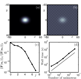
Fig. 5: Convergence of the Newton-GMRES solver. A stationary localised solution $u_{\ast}$ of IM is shown in panel (a). The solution is perturbed to obtain an initial guess $u_{0}=u_{\ast}+0.8\sin x\cos y$, shown in panel (b), and then the Newton-GMRES solver is used to converge back to $u_{\ast}$. Convergence is measured with the relative residual $\|\mathbf{F}(\mathbf{u}_{j})\|_{2}/\|\mathbf{F}(\mathbf{u}_{0})\|_{2}$, where $\mathbf{u}_{j}$ is the solution at the $j$th iteration (panel (c)). The experiment is repeated for several values of $N$ without any significant change to the convergence diagram, whereas the wall time for the numerical experiment scales linearly with the number of unknowns $N^{2}$, as reported in panel (d). Parameters of IM: $\theta=5.6$, $\mu=2.5$, $b=0.40$, $L=60$, $G_{0}=4.0$, $\alpha=1.0$, $\beta=4.0$, $\sigma=12.0$.

4.2 Snaking behaviour of radial and $\mathbf{D6}$ patterns

We now turn to the numerical continuation of localised states in IM, PDE4 and PDE8. The continuation parameter is the steepness $\mu$ of the sigmoidal firing rate, whereas the other parameters are fixed as follows: for IM, we choose $\theta=5.6$, $b=0.40$, $L=60$, $G_{0}=10^{-4}$, $\alpha=1.0$, $\beta=1.0$, $\sigma=\sqrt{10}$; for the PDE4 model, we use $\theta=5.6$, $R=60$, $G_{0}=0$ with fitting parameters for $\widehat{w_{4}}$ in Eq. (9) given by $A=1.225$, $B=0.1398$, $M=1.2183$; for the PDE8 model we use again $\theta=5.6$, $R=60$, $G_{0}=0$ with fitting parameters for $\widehat{w_{8}}$ in Eq. (11) given by $A=0.8510$, $B=0.6626$, $M=0.6653$, $C=0.3$ and $D=10$. We remark that translation invariance is removed in the IM by the negligible external input $G_{0}$ while in PDE4 and PDE8 this is achieved by the boundary conditions of the problems (17) and (19), so we choose $G_{0}=0$. In the present section we focus on the no- (or equivalent negligible-) input case which should be well understood before the addition of an input. In Sec. 5.2 we will provide examples of the model behaviour with input and discuss the implications.

The bifurcation points in the diagrams presented in this section will be labelled as follows. $F$ represents a fold bifurcation and $P$ a spatial-symmetry-breaking bifurcation from a radial state. Superscripts indicate the symmetry properties of the bifurcation, where $R$ represents a bifurcation on a branch with radially symmetric solutions and $\mathbf{D6}$ represents a bifurcation on a branch of $\mathbf{D6}$-symmetric solutions The labels $l$ and $r$ in the subscripts for fold bifurcations indicate whether the fold occurs on the left or right of the snaking structure. The indices $n$ in the subscripts indicate the ordering moving up the snaking structure. On radial branches $n$ corresponds to the number of rings around a central spot solution, for example, on the branch between $F^{R}_{l1}$ and $F^{R}_{r1}$ there is one ring around a central spot. On $\mathbf{D6}$-branches there are $n(n+1)/2\times 6$ additional spots glued around a central spot, for example, on the branch between $F^{\mathbf{D}6}_{l1}$ and $F^{\mathbf{D}6}_{r1}$ the solution has a total of 7 spots.

4.2.1 PDE4 results and comparison with IM

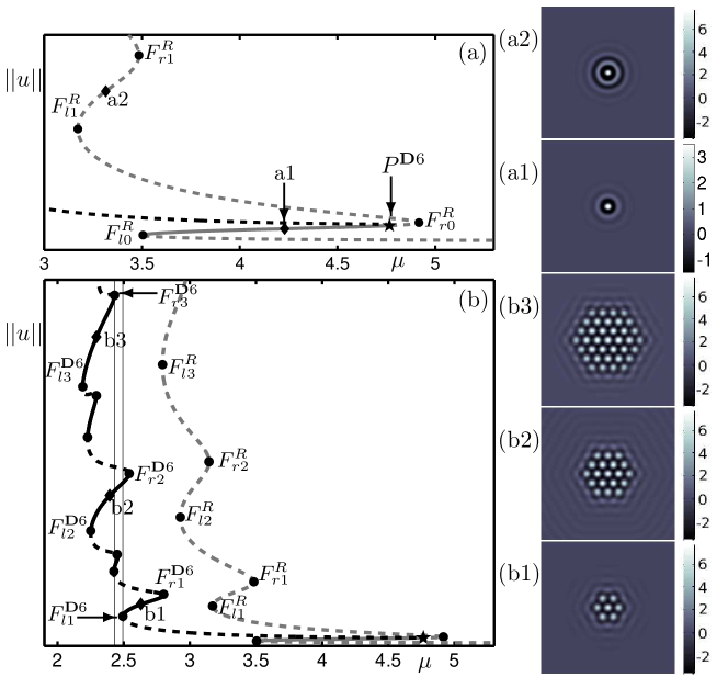
Fig. 6: Snaking of radially- and $\mathbf{D6}$-symmetric localised solutions in terms of $\mu$ for PDE4. Radial branches are grey curves and $\mathbf{D6}$ branches are black; stable segments are solid and unstable segments are dashed. Bifurcations labelled $F$ and $P$ are discussed in the text. (a): Detail of radial branch from (b); points labelled a1 and a2 correspond to planar plots showing a stable spot solution and an unstable spot-with-ring solution, respectively. (b): Global structure showing radial and $\mathbf{D6}$ branches; points labelled b1, b2 and b3 correspond to planar plots showing $7$-spot, $19$-spot and $37$-spot solutions, respectively. Thin vertical lines discussed in text. Parameters given at the beginning of Sec. 4.2.

We discuss both radially- and $\mathbf{D6}$-symmetric localised solutions of PDE4 with connectivity function defined via Eq. (9). Other solution branches with different symmetry properties do exist but these are only discussed for IM in Sec. 4.3. An unstable radial spot solution bifurcates from the trivial state $u=0$ at a Turing instability with $\mu$-value to the right of the range shown in the subsequent diagrams. It is this unstable radial spot branch that appears in the bottom right of Fig. 6(a) and (b).

Figure 6(b) shows the snaking structure for radial and $\mathbf{D6}$ branches. We first focus on the radial branch, detail of which is shown in panel (a). A radial spot branch enters the diagram in the bottom-right-hand corner and undergoes a fold at $F^{R}_{l0}$. The radial spot solution existing on the branch segment between $F^{R}_{l0}$ and $F^{R}_{r0}$ is plotted in panel (a1). This solution is stable between $F^{R}_{l0}$ and $P^{\mathbf{D}6}$. At $P^{\mathbf{D}6}$ on the radial branch a $\mathbf{D6}$ instability produces the bifurcating branch of $\mathbf{D6}$-symmetric solutions that leaves panel (a) in the bottom-left-hand corner. Beyond $P^{\mathbf{D}6}$ the radial branch is unstable and undergoes a further fold $F^{R}_{r0}$. After another fold $F^{R}_{l1}$ a ring has formed around the radial spot. The spot with ring solution existing on the branch segment between $F^{R}_{l1}$ and $F^{R}_{r1}$ is shown in panel (a2). The branch remains unstable and undergoes a series of further folds ($F^{R}_{l2}$, $F^{R}_{r2}$, $F^{R}_{l3}$, etc) adding additional rings as is shown in panel (b).

The $\mathbf{D6}$-symmetric branch that bifurcates from the radial branch at $P^{\mathbf{D}6}$ also undergoes a series of fold bifurcations as shown in Fig. 6(b). In this case a series of additional spots are added to the central spot in a configuration that preserves the $\mathbf{D6}$-symmetry. Planar plots in panels (b1), (b2) and (b3) show the stable $7$-spot, $19$-spot and $37$-spot solutions that exist on the branch segments between the fold pairs $(F^{\mathbf{D}6}_{l1},F^{\mathbf{D}6}_{r1})$, $(F^{\mathbf{D}6}_{l2},F^{\mathbf{D}6}_{r2})$ and $(F^{\mathbf{D}6}_{l3},F^{\mathbf{D}6}_{r3})$, respectively. There are further intermediate stable branch segments between pairs of fold bifurcations that have not been labelled. On the stable segment that can be found between $F^{\mathbf{D}6}_{r1}$ and $F^{\mathbf{D}6}_{l2}$, there exists a $13$-spot solution for which one spot has been glued on the long edge of each of the six sides of the solution shown in panel (b1). Similarly, on the stable segment that can be found between $F^{\mathbf{D}6}_{r2}$ and $F^{\mathbf{D}6}_{l3}$, there exists a $25$-spot solution for which two spots have been glued on the long edge of each of the six sides of the solution shown in panel (b2).

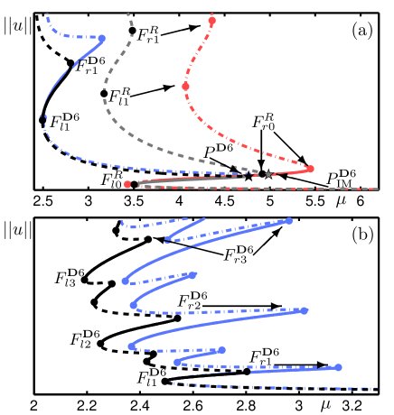
Fig. 7: Comparison between the solution branches of PDE4 (greyscale) and IM (colour). Black curves and grey correspond to the PDE approximation and have the line style and labelling conventions as Fig. 6. Corresponding radial and $\mathbf{D6}$ solution branches from IM are plotted as dash-dot curves in red and blue, respectively; stability is not indicated and folds not labelled on these branches. (a): Detail close to the spatial-symmetry-breaking bifurcation $P^{\mathbf{D}6}$; the corresponding bifurcation for IM is labelled $P^{\mathbf{D}6}_{\textrm{IM}}$. (b): Detail of the $\mathbf{D6}$ snaking structure. Parameters given at the beginning of Sec. 4.2.

The same radially- and $\mathbf{D6}$-symmetric branches shown in the previous section have been computed for IM. Here we test the accuracy of PDE4 both qualitatively in terms of the types of solutions produced and their bifurcations, and quantitatively in terms of the parameter ranges for which the different solution types persist. We are also interested to see whether the relative ranges of existence for different types of solution is consistent between PDE4 and IM.

Figure 7(a) and (b) both show detail from Fig. 6(b) with the same curves reproduced for PDE4 with the same line style and labelling conventions. Also plotted (in colour) are the equivalent curves computed for IM, where the equivalent of $P^{\mathbf{D}6}$ in IM is $P^{\mathbf{D}6}_{\textrm{IM}}$. The first major point to make is that in terms of the types of solution encountered, the series of bifurcations encountered and the stability of each branch segment, there is an exact agreement between PDE4 and IM. Furthermore, the quantitative agreement on the radial branch is good up until the fold point $F^{R}_{r1}$. Above $F^{R}_{r1}$, the radial branch for PDE4 makes a large excursion away from the IM branch and the branches remain well separated as the snaking continues; see panel (a). Similarly, for the $\mathbf{D6}$ branch the level of agreement is good up to $F^{\mathbf{D}6}_{r1}$ above which PDE4 branch deviates and remains well separated from the IM branch; see panel (b). The range of existence in $\mu$ for each stable branch segment on the $\mathbf{D6}$ branch is greatly under estimated by PDE4.

We now highlight a key qualitative difference between the bifurcation diagrams for PDE4 and IM. In IM, there is a range of $\mu\in[2.5,3.0]$ for which the stable branch segments corresponding to $7$-spot, $19$-spot and $37$-spot all overlap. This is not the case for PDE4, in particular, the branch segments corresponding to stable $7$-spot and $37$-spot solutions between the fold-pairs $(F^{\mathbf{D}6}_{l1},F^{\mathbf{D}6}_{r1})$ and $(F^{\mathbf{D}6}_{l3},F^{\mathbf{D}6}_{r3})$ do not overlap. This can be seen by the fact that $F^{\mathbf{D}6}_{r3}$ occurs at a smaller $\mu$-value (indicated by the first thin vertical line in Fig. 6(b)) than $F^{\mathbf{D}6}_{l1}$ (indicated by the second thin vertical line). This organisation of the solutions in parameter space is qualitatively inconsistent with IM.

4.2.2 PDE8 results and comparison with IM

Figure 8(a) shows branches of both radially- and $\mathbf{D6}$-symmetric solutions of PDE8. Globally the bifurcation diagram is the same as that of PDE4 in terms of the types of solution observed and the sequence of bifurcation encountered. There is an important difference between PDE4 and PDE8 in terms of the organisation in parameter space of the solution branches. For PDE4, there is no overlap in parameter ranges for which the $7$- and $37$-spot branches are stable; see the two vertical lines in Fig. 6 and note that $F^{\mathbf{D}6}_{r3}$ occurs before $F^{\mathbf{D}6}_{l1}$ in this case. In the PDE8 case, as shown in Fig. 8(a), there is an overlap in the parameter ranges as indicated by the grey shaded region. This organisation of the solution branches in parameter space is now consistent with the full model as shown in panel (c). Indeed PDE8 provides better agreement with IM; the branches remain close for both the radial and the $\mathbf{D6}$ branches as we move up the snaking structure as can be seen in panels (b) and (c). We note that when compared with IM, the upper section of the radial branch occurs at smaller values of $\mu$ for PDE4 and at larger values of $\mu$ for PDE8; compare Fig. 6(a) with Fig. 8(b).

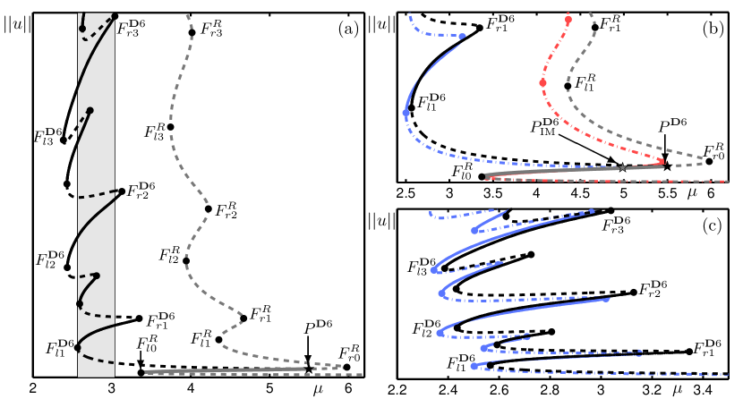
Fig. 8: Snaking of radially- and $\mathbf{D6}$-symmetric localised solutions in terms of $\mu$ for PDE8 (greyscale) and comparison with IM (colour). Black and grey curves correspond to the PDE approximation and have the line style and labelling conventions as Fig. 6. Corresponding radial and $\mathbf{D6}$ solution branches from the full model are plotted as dash-dot curves in red and blue, respectively; stability is not indicated and folds not labelled on these branches. (a): Global snaking diagram for PDE8. (b): Detail close to the spatial-symmetry-breaking bifurcation $P^{\mathbf{D}6}$; the corresponding bifurcation in the full model is labelled $P^{\mathbf{D}6}_{\textrm{IM}}$. (c): Detail of the $\mathbf{D6}$ snaking structure. Parameters given at the beginning of Sec. 4.2.

4.3 Snaking of $\mathbf{D2}$, $\mathbf{D3}$ and $\mathbf{D4}$ patterns in IM

In this section we discuss several patterns that possess neither radial nor $\mathbf{D6}$ symmetry. For non-radial patterns discussed so far in this article, see Fig. 6(b1)–(b3), the individual spots lie on a regular hexagonal lattice. However, there exist an infinite number of stable configurations that conform to the same lattice spacing but without the full $\mathbf{D6}$ symmetry; here we present two such examples. We also present one further example of a stable configuration that does not conform to the regular hexagonal lattice.

4.3.1 Three-spot pattern ($\mathbf{D3}$)

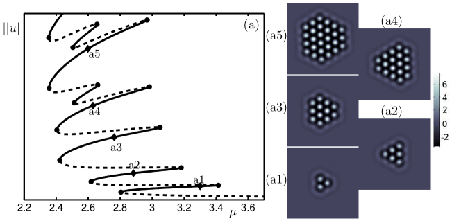
Fig. 9: Snaking of patterns with $\mathbf{D3}$ symmetry built around a triangular-organised, three-spot solution. Line style conventions for stability as in Fig. 6. Parameters for IM as given at the beginning of Sec. 4.2.

Figure 9 shows the snaking of $\mathbf{D3}$-symmetric patterns about a three-spot solution. The unstable branch that enters panel (a) in the bottom-right-hand corner reconnects to the trivial state $u=0$ at the Turing instability (not shown). The panels (a1)–(a5) show stable solutions on the first five full excursions in $\mu$ of the snaking structure. The existence of three-spot (see panel (a1)) and twelve-spot (see panel (a3)) solutions for PDE4 with connectivity given by Eq. (9) was shown in [43]. Here we have shown that these solutions exist in IM and that they form part of a larger snaking structure.

4.3.2 Two-spot pattern ($\mathbf{D2}$)

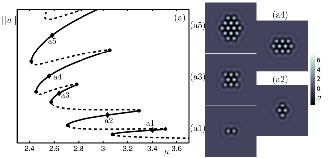
Fig. 10: Snaking of patterns with $\mathbf{D2}$ symmetry built around a two-spot solution. Line style conventions for stability as in Fig. 6. Parameters for IM given at the beginning of Sec. 4.2.

Similarly, there is an unstable two-spot solution that connects to the trivial state $u=0$ at the Turing instability (not shown). Figure 10(a) shows that this solution also undergoes a sequence of fold bifurcations giving rise to larger $\mathbf{D2}$-symmetric patterns. We note that the spacing between the spots in these patterns still conforms to the regular hexagonal lattice. The panels (a1)–(a5) show solutions on the first five stable branch segments moving up the snaking structure; we note that the pattern (a3) is on an intermediate branch that does not make a full excursion in $\mu$.

4.3.3 Quincunx pattern ($\mathbf{D4}$)

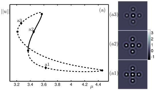
Fig. 11: Isola of five-spot solution organised in a quincunx configuration. Line style conventions for stability as in Fig. 6. Parameters for IM given at the beginning of Sec. 4.2.

We show in Fig. 11(a2) a stable configuration that lies on a square lattice but with a spacing between the spot peaks that is double that of the hexagonal-lattice solutions encountered thus far. The solution is formed by five spots that interact at the first excitatory peak away from $0$ in the connectivity function (7) as shown in Fig. 3(d). The configuration of four spots forming a square with an additional spot in the center is typically referred to as a quincunx pattern that is found, for example, on dice and dominoes. As shown in Fig. 10(a) these solutions exist on an isola in parameter space where other branches, see panels (a1) and (a3), are unstable. Although the pattern does not undergo snaking-type behaviour it may be possible to construct larger patterns on the double-spaced square lattice.

5 Discussion

5.1 Summary

This paper explores patterns of localised activity in the neural field equation posed on the Euclidean plane with a smooth firing rate function. The choice of connectivity function is an important factor in determining whether, the localised behaviour found is restricted to individual spots, or whether multiple interacting spots can form coherent localised patterns. In [30] localised states were studied in a model with a radially-symmetric wizard-hat connectivity function describing local excitation and lateral inhibitions in the Euclidean plane. When spot solutions were tracked using numerical continuation no snaking behaviour was observed, i.e. the only steady states found consisted of a single spot. The radially symmetric connectivity function studied here and shown in Fig. 3(d)) features local excitation, lateral inhibition and long-range bands of excitation that decay with distance. Indeed, the distance between excitation peaks fixes a spatial scale that allows for regular spatial interactions and the formation of larger patterns of activity. In [43] it was shown that multiple-spot patterns could be obtained all with the common property of the peaks lying on a regular hexagonal lattice with spacing determined by the connectivity function. One of the main aims in the present article was to show how these solutions are connected in parameter space and how patterns with varying spatial extent grow via the mechanism of homoclinic snaking.

The results presented in [43] relied on working with an approximated connectivity function (see Fig. 4(a) and (b)) that allowed for solutions the full integral neural field equation to be studied in an equivalent fourth-order PDE . The initial parts of the results section are concerned with the relative agreement between solutions to the integral model and equivalent PDE formulations with approximated connectivity functions. We pursue the problem numerically by investigating the level of agreement in terms of an entire bifurcation diagram rather than comparing individual solutions at fixed parameter values. We compared both radially symmetric and $\mathbf{D6}$-symmetric solution branches and found that the qualitative difference of the zero-mode in the Fourier domain for the approximated connectivity used in the fourth-order model (see Fig. 4(b)) led to significant discrepancies in the existence ranges of solution branches, in particular for solutions with a larger spatial extent. We demonstrated that the improved approximation of the connectivity function shown in Fig. 4(c) and (d), leading to an eighth-order PDE, provides a better agreement across the full bifurcation diagram. In particular, the eigth-order model captures the key feature of there being a specific parameter range in which multiple solutions coexist, each solution with a different spatial extent. It was not possible to capture this feature with the fourth-order approximation. We conclude that, although equivalent PDE formulations have proved to be a useful tool for the study of neural fields, it is important to ensure close agreement between the connectivity functions in the Fourier domain. Increasing the order of the PDEs used allows for improvements in this agreement. We believe that, while converting the integral formulation to higher-order PDEs could be useful in analytical studies, numerical calculations of these systems should be approached without resorting to PDE formulation where possible. In passing, we point out that the methodology proposed here for the integral model is applicable to inhomogeneous synaptic kernels, provided that the convolution structure of the integral is preserved. Furthermore, we point out that here we have used the standard Newton-GMRES method mainly for its simplicity, but more sophisticated choices are also possible [39].

Having investigated radial and $\mathbf{D6}$ solutions with PDE formulations and compared the results with the full integral model, we proceeded to give an account of other types of solutions that, when path-followed with numerical continuation lead to patterns with different underlying symmetry properties. We worked with the full integral model and showed that patterns with $\mathbf{D2}$ and $\mathbf{D3}$ symmetry also give rise to snaking behaviour, generating spatial patterns with variable spatial extent. All the solutions of this type, including those shown earlier with $\mathbf{D6}$-symmetry, have the common feature of the individual spots lying on a regular hexagonal lattice. Furthermore, these solutions of variable spatial extent exist within roughly the same ranges of the parameter $\mu$. As the snaking diagram is ascended, new spots are glued to long edges of the pattern in a regular fashion. We note the existence of an arbitrary number of intermediate branches not shown in our bifurcation diagrams where symmetries can be broken via the (simultaneous) addition or subtraction of one (or more spots). We expect these solutions to lie on intermediate branches that are stable over ranges smaller than the full excursions in the main snaking structure.

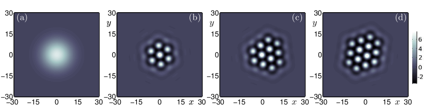
Fig. 12: Model simulations with input given by Eq. (8) with $\alpha=\beta=1$. The simulations are performed with $\mu=2.4$. (a) The Gaussian-bump input plotted with $\sigma=10$ and $G_{0}=6$ ($G_{0}=1.5$ used in the simulations). (b): Case with $\sigma=9.0$, the model converges to a $7$s-spot solution that is a modified version of the state shown in Fig. 6(b1) (c): Case with $\sigma=9.5$, the model converges to a $12$s-spot solutions that is a modified version of the state shown in Fig. 9(a3) (d): Case with $\sigma=10.0$, the model converges to a $14$s-spot solutions that is a modified version of the state shown in Fig. 10(a5). Other model parameters (for IM) given at the beginning of Sec. 4.2.

5.2 Localised patterns with input

The numerical bifurcation analysis presented in this paper opens up the possibility to investigate the spread of cortical activity with inputs. An important principle in studying the neural field equation is that weak inputs to the equations should drive the system to states that are already solutions to the underlying equations without input. The bifurcation study presented here allows us to identify the types of solution that we may expect to encounter for localised inputs and the relevant parameter regime in which they occur. Two criteria need to be satisfied when identifying a suitable operating regime, 1) the model should only produce the trivial homogeneous state $u=0$ before an input is introduced and 2) when an input is introduced, the model should be driven to one of the underlying non-trivial solutions. We have shown that, for the full integral model, there is an accumulation of fold bifurcations at around $\mu=2.4$ representing the first point for which localised patterns can be observed. Both criteria are satisfied when the model is operated just before these fold points. Introducing a weak input the system can be driven to states that have a spatial extent corresponding to that of the input. Figure 12(a) shows the profile of the input used in a series of simulations that were initiated with the $u=0$ state plus a small random perturbation across the entire spatial domain. Figures 12(b), (c) and (d) show the result of three $150$ time unit simulations, each with different spatial extent for the input. In each case, the trivial state $u=0$ is no longer stable and the system naturally selects one of the solutions described in the early bifurcation analysis. As the spatial extent of the input increases, the size of the pattern selected by the model increases and this is an important consequence of the corresponding solutions existing as part of a snaking structure. The computational framework presented in this article will allow for the relationship between model inputs and spatially localised patterns to be investigated in future work.

5.3 Patterns on other lattices and parametric forcing

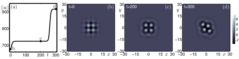
Fig. 13: Symmetry breaking of weakly unstable solution on a square lattice at $\mu=3.2$. (a): Evolution of L2 norm. (b): Initial condition given by Eq. (22). (c): Weakly unstable solution. (d): Stable solution. Parameters (for IM) given at the beginning of Sec. 4.2.

The multi-spot solutions described in this article all have the common feature of the activated peaks falling onto a regular hexagonal lattice. Indeed, this has been found to be the default way for the radial symmetry to be broken in pattern forming systems, notably the archetypal Swift-Hohenberg equation [46]. We also investigated whether it is possible to find other states that do not conform to the regular hexagonal lattice. In Fig. 11 an example of a solution with $\mathbf{D4}$ symmetry was shown that consists of five spots interacting at double the standard separation between excitation peaks. We found this solution to exist on an isola and not undergo snaking so as to find larger patterns tiling the plane with the same spacing. We also attempted to converge solutions with $\mathbf{D4}$ symmetry that have the regular spacing between peaks. A suitable initial condition to find such solutions is given by Eq. (22) chosen such that there is a depression at $(x,y)=(0,0)$ and the surrounding square-lattice pattern decays away from the origin, see Fig. 13(b). In an appropriate parameter range these states appear to converge to stable patterns. However, we found the patterns to be weakly unstable, finally converging to a pattern on a hexagonal lattice after a long transient. Figure 13(a) shows a time-course of the L2 norm from a simulation with the initial condition shown in panel (b). The model reaches the apparently stable $\mathbf{D4}$ configuration after approximately $30$ time units (panel (c)) before finally converging after $230$ time units to the $\mathbf{D2}$-symmetric pattern (panel (d)) that was previously identified in Fig. 10(a2). It would be possible to stabilise such weakly unstable solutions with the use of parametric forcing, by introducing small modulations that encourage interactions on a fixed lattice in cortical space. In the neural field equations this is typically referred to as inhomogeneous neural media; travelling waves, travelling fronts, periodic patterns and pulsating fronts have been studied with such modulations [7, 24, 20]. The study of localised states in this context would be an interesting future direction. Furthermore, stable quasi-periodic patterns have been obtained in the Swift-Hohenberg equation through parametric forcing [37]. The question of introducing orientation-preference tilings on square and hexagonal lattices was addressed in [4]. However, one is restricted in the number of orientations that can be equally represented with such tilings, (two and three, respectively). Parametric forcing on a quasi-periodic lattice is of particular interest in the neural field equations as this could allow for near-continuous representations of features in a model without an abstracted feature space.

6 Conclusions

The organisation in parameter space of localised structures consisting of multiple spots has been revealed for the first time in planar neural field equations. In order to find such behaviour, one must choose a connectivity function with an excitatory peak away from the origin that fixes a regular spatial scale of interactions between spots. As localised solutions are path-followed using numerical continuation we find that these structures grow in a series of fold bifurcations through the mechanism of homoclinic snaking that has been well-studied in the Swift-Hohenberg equation. A numerical strategy has been proposed to perform a numerical bifurcation analysis without resorting to a PDE formulation, but taking advantage of matrix-free Newton-Krylov nonlinear solvers combined with a pseudospectral evaluation of the right-hand side. The novel application of these methods to the neural field equations allowed for numerical continuation to be applied to the full integral form of the model. Previous studies in 2D have relied exclusively on PDE approximations of the connectivity functions; here we demonstrated that these approximations can give a very close agreement with the full integral model if a sufficiently high-order approximation is taken. The numerical schemes presented here will allow for future studies of the neural field equations to use connectivity functions defined either directly in the real domain or the Fourier domain without recourse to PDE methods, provided that the sigmoidal firing rate be smooth and that the integral formulation can be expressed as a convolution (this extends also to inhomogeneous firing rates).

The neural field studied in the present paper can be considered as a model of the visual cortex and the localised patterns studied without inputs can be related to visual hallucinations that can be localised in the visual field [54]. Furthermore, we have shown that the localised states computed in our bifurcation analysis are exactly the types of solutions selected by the model in the presence of weak inputs. The persistence of these localised structures in the presence of a model input is new. This future direction will be of particular interest for the study of localised patterns of activity that have been observed in the primary visual cortex [17] with localised visual input.

Appendix A Analytic expressions for initial conditions

Figure 2(a) shows the initial condition given by

$$u(x,y)=A\exp\bigg{(}-\frac{x^{2}+y^{2}}{L}\bigg{)},$$ (20)

with $A=6$ and $L=5.77$; subsequent panels (b) and (c) show a transient state after $1$ time unit and the stable steady state after $15$ time units. Figure 2(d) shows the initial condition given by

$$u(x,y)=A\exp\bigg{(}-\frac{x^{2}+y^{2}}{L}\bigg{)}\left[\cos(x)+\cos\left(\frac{1}{2}x+\frac{\sqrt{3}}{2}y\right)+\cos\left(-\frac{1}{2}x+\frac{\sqrt{3}}{2}y\right)\right],$$ (21)

with $A=2$ and $L=100$; subsequent panels (e) and (f) show a transient state after $1$ time unit and the stable steady state after $15$ time units. Figure 13(b) shows the initial condition given by

$$u(x,y)=2\exp\bigg{(}-\frac{x^{2}+y^{2}}{L}\bigg{)}(-\cos x-\sin y),$$ (22)

with $A=2$ and $L=65$; subsequent panels (c) and (d) show transient states after $200$ and $300$ time units, respectively. The $L_{2}$-norm is plotted over this time course in panel (a).

References

- [1] S. Amari, Homogeneous nets of neuron-like elements, Biological Cybernetics, 17 (1975), pp. 211–220.
- [2] S.-I. Amari, Dynamics of pattern formation in lateral-inhibition type neural fields, Biological Cybernetics, 27 (1977), pp. 77–87.
- [3] D. Avitabile, D. Lloyd, J. Burke, E. Knobloch, and B. Sandstede, To snake or not to snake in the planar swift-hohenberg equation, SIAM J. Appl. Dyn. Syst., 9 (2010), pp. 704–733.
- [4] T. Baker and J. Cowan, Spontaneous pattern formation and pinning in the primary visual cortex, Journal of Physiology-Paris, 103 (2009), pp. 52–68.
- [5] M. Beck, J. Knobloch, D. Lloyd, B. Sandstede, and T. Wagenknecht, Snakes, ladders, and isolas of localised patterns, SIAM J. Math. Anal, 41 (2009), pp. 936–972.
- [6] R. Ben-Yishai, R. Bar-Or, and H. Sompolinsky, Theory of orientation tuning in visual cortex, Proceedings of the National Academy of Sciences, 92 (1995), pp. 3844–3848.
- [7] P. Bressloff, Traveling fronts and wave propagation failure in an inhomogeneous neural network, Physica D: Nonlinear Phenomena, 155 (2001), pp. 83–100.
- [8] , Spatiotemporal dynamics of continuum neural fields, Journal of Physics A: Mathematical and Theoretical, 45 (2012).
- [9] P. Bressloff, J. Cowan, M. Golubitsky, P. Thomas, and M. Wiener, Geometric visual hallucinations, euclidean symmetry and the functional architecture of striate cortex, Phil. Trans. R. Soc. Lond. B, 306 (2001), pp. 299–330.
- [10] P. Bressloff and Z. Kilpatrick, Two-dimensional bumps in piecewise smooth neural fields with synaptic depression, SIAM Journal on Applied Mathematics, 71 (2011), pp. 379–408.
- [11] J. Burke and E. Knobloch, Homoclinic snaking: structure and stability, Chaos, 17 (2007), p. 7102.
- [12] , Snakes and ladders: localized states in the swift–hohenberg equation, Physics Letters A, 360 (2007), pp. 681–688.
- [13] P. Buzás, U. Eysel, P. Adorján, and Z. Kisvárday, Axonal topography of cortical basket cells in relation to orientation, direction, and ocular dominance maps, The Journal of comparative neurology, 437 (2001), pp. 259–285.
- [14] C. Canuto, M. Hussaini, A. Quarteroni, and T. Zang, Spectral Methods: Fundamentals in Single Domains, Springer-Verlag, Berlin, 2006.
- [15] A. Champneys and B. Sandstede, Numerical computation of coherent structures, in Numerical Continuation Methods for Dynamical Systems, Springer, 2007, pp. 331–358.
- [16] S. Chapman and G. Kozyreff, Exponential asymptotics of localized patterns and snaking bifurcation diagrams., Physica D, 238 (2009), pp. 319–354.
- [17] F. Chavane, D. Sharon, D. Jancke, O. Marre, Y. Frégnac, and A. Grinvald, Lateral spread of orientation selectivity in v1 is controlled by intracortical cooperativity, Frontiers in Systems Neuroscience, 5 (2011).
- [18] C. Colby, J. Duhamel, and M. Goldberg, Oculocentric spatial representation in parietal cortex, Cereb. Cortex, 5 (1995), pp. 470–481.
- [19] S. Coombes, Waves, bumps, and patterns in neural fields theories, Biological Cybernetics, 93 (2005), pp. 91–108.
- [20] S. Coombes and C. Laing, Pulsating fronts in periodically modulated neural field models, Physical Review E, 83 (2011), p. 011912.
- [21] S. Coombes, G. Lord, and M. Owen, Waves and bumps in neuronal networks with axo-dendritic synaptic interactions, Physica D: Nonlinear Phenomena, 178 (2003), pp. 219–241.
- [22] S. Coombes, H. Schmidt, and D. Avitabile, Neural Field Theory, Springer, 2013, ch. Spots: Breathing, drifting and scattering in a neural field model.
- [23] S. Coombes, H. Schmidt, and I. Bojak, Interface dynamics in planar neural field models, Journal of mathematical neuroscience, (2012).
- [24] S. Coombes, N. Venkov, L. Shiau, I. Bojak, D. Liley, and C. Laing, Modeling electrocortical activity through improved local approximations of integral neural field equations, Physical Review E, 76 (2007), p. 051901.
- [25] P. Coullet, C. Riera, and C. Tresser, Stable static localized structures in one dimension, Phys. Rev. Lett., 84 (2000), pp. 3069–3072.
- [26] A. Elvin, C. Laing, R. McLachlan, and M. Roberts, Exploiting the hamiltonian structure of a neural field model, Physica D: Nonlinear Phenomena, 239 (2010), pp. 537–546.
- [27] G. Ermentrout, Neural networks as spatio-temporal pattern-forming systems, Reports on Progress in Physics, 61 (1998), pp. 353–430.
- [28] G. Ermentrout and J. Cowan, A mathematical theory of visual hallucination patterns, Biological Cybernetics, 34 (1979), pp. 137–150.
- [29] G. Faye, J. Rankin, and P. Chossat, Localized states in an unbounded neural field equation with smooth firing rate function: a multi-parameter analysis, Journal of Mathematical Biology, (2012).
- [30] G. Faye, J. Rankin, and D. Lloyd, Localized radial bumps of a neural field equation on the euclidean plane and the poincaré disk, Nonlinearity, (accepted) (2012).
- [31] S. Folias and P. Bressloff, Breathing pulses in an excitatory neural network, SIAM Journal on Applied Dynamical Systems, 3 (2004), pp. 378–407.
- [32] , Breathers in two-dimensional neural media, Physical Review Letters, 95 (2005), p. 208107.
- [33] S. Funahashi, C. Bruce, and P. Goldman-Rakic, Mnemonic coding of visual space in the monkey’s dorsolateral prefrontal cortex, J. Neurophysiol., 61 (1989), pp. 331–349.
- [34] B. Gutkin, G. B. Ermentrout, and J. O’Sullivan, Layer 3 patchy recurrent excitatory connections may determine the spatial organization of sustained activity in the primate prefrontal cortex, Neurocomputing, 32 (2000), pp. 391–400.
- [35] D. Hansel and H. Sompolinsky, Modeling feature selectivity in local cortical circuits, Methods of neuronal modeling, (1997), pp. 499–567.
- [36] F. Haudin, R. Rojas, U. Bortolozzo, S. Residori, and M. Clerc, Homoclinic snaking of localized patterns in a spatially forced system, Physical Review Letters, 107 (2011), p. 264101.
- [37] G. Iooss and A. Rucklidge, On the existence of quasipattern solutions of the swift–hohenberg equation, Journal of Nonlinear Science, 20 (2010), pp. 361–394.
- [38] C. Kelley, Iterative methods for linear and nonlinear equations, Society for Industrial and Applied Mathematics, 1995.
- [39] , Solving nonlinear equations with Newton’s method, Society for Industrial and Applied Mathematics, 2003.
- [40] E. Knobloch, Spatially localized structures in dissipative systems: open problems, Nonlinearity, 21 (2008), pp. T45–T60.
- [41] C. Laing, Spiral waves in nonlocal equations, SIAM Journal on Applied Dynamical Systems, 4 (2005), pp. 588–606.
- [42] , Neural Field Theory, Springer, 2013, ch. PDE Methods for Two-Dimensional Neural Fields.
- [43] C. Laing and W. Troy, PDE methods for nonlocal models, SIAM Journal on Applied Dynamical Systems, 2 (2003), pp. 487–516.
- [44] C. Laing, W. Troy, B. Gutkin, and G. Ermentrout, Multiple bumps in a neuronal model of working memory, SIAM J. Appl. Math., 63 (2002), pp. 62–97.
- [45] D. Lloyd and B. Sandstede, Localized radial solutions of the Swift-Hohenberg equation, Nonlinearity, 22 (2009), pp. 485–524.
- [46] D. Lloyd, B. Sandstede, D. Avitabile, and A. Champneys, Localized hexagon patterns of the planar Swift–Hohenberg equation, SIAM J. Appl. Dynam. Syst., 7 (2008), pp. 1049–1100.
- [47] S. McCalla and B. Sandstede, Snaking of radial solutions of the multi-dimensional swift-hohenberg equation: A numerical study, Physica D: Nonlinear Phenomena, 239 (2010), pp. 1581–1592.
- [48] I. Nickolls, J.and Buck, M. Garland, and K. Skadron, Scalable parallel programming with cuda, Queue, 6 (2008), pp. 40–53.
- [49] E. Niebur and F. Wörgötter, Design principles of columnar organization in visual cortex, Neural Computation, 6 (1994), pp. 602–614.
- [50] M. Owen, C. Laing, and S. Coombes, Bumps and rings in a two-dimensional neural field: splitting and rotational instabilities, New Journal of Physics, 9 (2007), pp. 378–401.
- [51] H. Sakaguchi and H. Brand, Stable localized solutions of arbitrary length for the quintic Swift-Hohenberg equation, Physica D, 97 (1996), pp. 274–285.
- [52] , Localized patterns for the quintic complex Swift-Hohenberg equation, Physica D, 117 (1998), pp. 95–105.
- [53] T. Schneider, J. Gibson, and J. Burke, Snakes and ladders: localized solutions of plane couette flow, Physical review letters, 104 (2010), p. 104501.
- [54] R. Siegel, Hallucinations., Scientific American, (1977).
- [55] J. Taylor, Towards the networks of the brain: from brain imaging to consciousness, Neural Networks, 12 (1999), pp. 943–959.
- [56] L. Trefethen, Spectral methods in MATLAB, vol. 10, Society for Industrial and Applied Mathematics, 2000.
- [57] H. Werner and T. Richter, Circular stationary solutions in two-dimensional neural fields, Biological Cybernetics, 85 (2001), pp. 211–217.
- [58] H. Wilson and J. Cowan, Excitatory and inhibitory interactions in localized populations of model neurons, Biophys. J., 12 (1972), pp. 1–24.
- [59] , A mathematical theory of the functional dynamics of cortical and thalamic nervous tissue, Biological Cybernetics, 13 (1973), pp. 55–80.
- [60] P. Woods and A. Champneys, Heteroclinic tangles and homoclinic snaking in the unfolding of a degenerate reversible hamiltonian-hopf bifurcation, Physica D: Nonlinear Phenomena, 129 (1999), pp. 147–170.