A numerical method for imaging of biological microstructures by VHF waves

Abstract

Imaging techniques give a fundamental support to medical diagnostics during the pathology discovery as well as for the characterization of biological structures. The imaging methods involve electromagnetic waves in a frequency range that spans from some Hz to GHz and over. Most of these methods involve scanning of wide human body areas even if only small areas need to be analyzed. In this paper, a numerical method to evaluate the shape of micro-structures for application in the medical field, with a very low invasiveness for the human body, is proposed. A flexible thin-wire antenna radiates the VHF waves and then, by measuring the spatial magnetic field distribution it is possible to reconstruct the micro-structure’s image by estimating the location of the antenna against a sensors panel. The typical inverse problem described above is solved numerically, and first simulation results are presented in order to show the validity and the robustness of the proposed approach.

1 Introduction

The support given by the imaging to medical diagnostics is fundamental during the pathology discovery as well as for biochemical characterization of biological structures [1]-[7]. The imaging methods involve electromagnetic waves in a frequency range that spans from some Hz to GHz and over. Hence, the understanding of biological structures response to the electromagnetic field is fundamental. The investigation of the interaction between healthy or pathological biological tissues and electromagnetic waves is a hot topic yet [8]. In fact,understanding how an electromagnetic wave interacts with the human body becomes increasingly important if one considers that the most of imaging methods involve scanning of wide areas of the human body, even if only small areas need to be analyzed. In this way, although a wide scanning allows to acquire a big amount of data by single exposition, also areas of the body not interested in the diagnostics are exposed to the waves, so increasing the invasiveness for the patient. For this reason, new imaging systems able to analyze only the area under diagnostics (confined scanning), are becoming more and more investigated. A big input to micro-imaging systems has been given by the micro-electronic technology, which allows the development of systems for the scanning of confined small areas. In fact, emitters and receivers (sensors) smaller and smaller can be made, so that the final size of the imaging systems as well as the wave’s spot become very small. Generally, the acquired data need to be appropriately elaborated extracting the imaging information by means of inverse optimization algorithms [3],[4],[7]. Through these algorithms high quality information can be extracted from the data acquired by the sensors, even if the quality of the sensor’s signal is low, because of their small area which may determine a significant amount of noise. In this paper a method to elaborate the shape of microstructures for application in the medical field is proposed. The method works with low power waves in the Very High Frequency (VHF) range, in order to achieve a low invasiveness for the human body. The method uses a system endowed with: a microtransmitter to emit a magnetic field, a sensors panel to acquire the spatial distribution of the magnetic field and an elaboration logic to acquire and elaborate the sensor’s signals. The microtransmitter radiates the VHF waves by means of a microantenna, which is able to take the shape of the target structure. If the micro-antenna is assumed to be a sequence of thin-wire interconnected short dipoles, then it is possible to reconstruct the micro-structure’s image by measuring the spatial distribution of the magnetic field. In fact, the shape reconstruction is possible by estimating the location of thin-wire antenna against the sensors panel. The recognition problem of the thin-wire antenna’s location by magnetic field can be addressed as an inverse problem. The thin-wire antenna is supposed to be a sequence of linear segments: given a model for the characterization of the magnetic field at a point in space (forward problem) and given a set of measurements of the magnetic field amplitude, it is possible to solve the inverse problem in terms of the distance of the antenna from the sensors panel. In this paper, preliminary results about the previous basic idea, are reported concerning two simulated scenarios. Namely, the spatial distribution of the emitted magnetic field is simulated through a numerical model based on the method of moments (MoM), where the first kind Fredhlom’s integral equation is solved by the point matching procedure [9]-[15]. The spatial distribution of the magnetic field is evaluated on an area equivalent to the area of the sensors panel. These magnetic field values are used as the measured input for the inverse problem. The Levenberg-Marquart algorithm [16], [17] is considered in solving the inverse problem by means of the minimization of the Euclidean distance between the measured field and the field generated by a given configuration of thinwire piecewise antenna. The numerical procedure involved by the algorithm rounds the entries of the Hessian matrix, step by step, and the location of the antenna’s segments can be estimated with high precision, so obtaining the image of the shape taken by the antenna. The paper is structured as follows. In section 2 the mathematical framework about the proposed method is presented. In section 3 some numerical results about reconstruction examples are discussed, then a conclusion about the method results and ongoing work complete the paper.

2 Numerical approach

The shape of a biological thin micro-structure can be estimated by means of an appropriate embedded emitting antenna and by measuring the spatial distribution of the opportune radiated electromagnetic field component. In particular, the magnetic field may be the best choice together with the selection of the appropriate work frequency range. The proposed approach is a typical inverse problem: the measured spatial distribution of the magnetic field emitted by a VHF thinwire antenna (i.e. with radius less than one hundredth of the maximum work wavelength) is the input, and the source shape reconstruction is the final target. The antenna is assumed to be a piecewise linear structure, i.e. a sequence of $\textit{N}_{\textit{b}}$ branches with uniform radius $\textit{r}_{\textit{cond}}$ and conductivity

$\sigma_{omega}$ . The antenna is fed at the point $P_{0}(x_{0},y_{0},z_{0})$ by a sinusoidal current source with known frequencyf and amplitude $I_{source}$. The spatial distribution of the magnetic field is detected by a sensors panel with M sensors distributed on its surface. As a first approximation, the surrounding medium is supposed to be homogeneous, isotropic, with conductivity $\sigma$, electric permittivity $\epsilon$ and magnetic permeability $\mu$. Under these assumptions, the shape reconstruction involves the minimization of an objective function shown in equation (1), by using an iterative procedure. Roughly speaking, step by step the iterative procedure looks for a set of segments coordinates that minimize the difference between the computed and measured magnetic field at sensor points.

$$min_{p}\left\{||H_{comp}(p)-H_{means}(p)||_{2}\right\}$$ (1)

In equation (1) $p=[(x_{1},y_{1},z_{1})...(x_{N_{b}},y_{N_{b}},z_{N_{b}})]^{T}$ is the vector of the cartesian coordinates of the antenna segments ends to be estimated, $H_{comp}$ is the vector of the magnetic field values at sensors points computed by assuming that the segments ends are located at p, and $H_{meas}$ is the vector with the measured magnetic field values. The values of $H_{comp}$ are calculated by the forward solver. The forward solver computes the amplitude of the magnetic field at a set of points, for a given signal source and antenna’s characteristics. More precisely, the current distribution along the antenna is evaluated by solving an appropriate integral equation in frequency domain, derived from Maxwell’s equations. Then, by using the relation that link the currents to the magnetic field, this latter can be calculated at the sensors points. The equations of the forward model is solved numerically. For the problem addressed in this case, the moments method (MoM) via point-matching procedure in the frequency domain, is performed . Note that, by this method the integral equations involved include the boundary conditions, so that only the emitter have to be discretized but not the problem’s domain. This means that each antenna’s branch needs to be split in a finite number of linear segments [9]-[14]. The problem formulation leads to a first kind Fredholm’s integral equation. In fact, by expressing the electric field $\vec{E}$ with the retarded magnetic vector potential $\vec{A}$, the source frequency $(\omega=2\pi f)$ and the scalar potential $\phi$, as shown in equation (2):

$$\vec{E}=-(\nabla\phi+j\omega\vec{A})$$ (2)

by introducing the boundary conditions by means of the per-unit-length surface impedance $\dot{z_{s}}$, the following equation holds:

$$\vec{\textbf{u}}\cdot\vec{E}=\dot{z_{s}}I_{s}$$ (3)

$-(\nabla\phi+j\omega\vec{A})_{tg}=z_{s}I_{s}$

in which tg indicates the component tangential to the wire surface, $I_{s}$ is the longitudinal current flowing into the conductor, concentrated on its axis $(\textbf{u}^{\prime}$ as the unit vector) because of the thin-wire assumption [9], [12], u is the unit vector tangential to the conductor’s surface, as shown in figure 1.

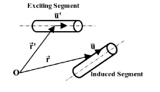
Figure 1: General thin-wire geometric references.

By using the relation between the magnetic vector potential $\vec{A}$ and the conduction current density, and the relation between the scalar electric potential $\phi$ and the free electric charges density, the well known electric field integral equation (EFIE) is obtained. Then, by integrating the EFIE along the surface of the conductor, the following modified EFIE is obtained [9], [12]:

$$\begin{array}[]{lll}j\omega\int_{L}\vec{\textbf{u}}\cdot\int_{\Omega}\mu I_{s}(l^{\prime})g(\vec{r},\vec{r^{\prime}})dl^{\prime}dl\\ \\ +\int_{L}\frac{\partial}{\partial l_{tg}}\frac{1}{j\omega\dot{\epsilon}}\int_{\Omega}\frac{dI_{s}(l^{\prime})}{dl^{\prime}}g(\vec{r},\vec{r^{\prime}})dl^{\prime}dl=\\ \\ \dot{z_{s}}\int_{L}I_{s}(\vec{r})dl\end{array}$$ (9)

Equation (9) is a general relation that depends only on thelongitudinal current and on geometrical quantities of the conductors constituting the thin-wire structures to be analyzed. In fact, $\Omega$ is the length of the exciting conductor, L is the length of the induced conductor, $\vec{r}$ and $\vec{r^{\prime}}$ are space position vectors of the observation and source points, respectively, $g(\vec{r},\vec{r^{\prime}})=\frac{e^{-k|\textbf{r}-\textbf{r'}|}}{4\pi|\textbf{r}-\textbf{r'}|}$ is the Green’s function in an unbounded region. The quantity $\dot{\epsilon}=\epsilon+j\omega\sigma$ take into account the complex medium permittivity and $\dot{k}=\sqrt{-\omega^{2}\mu\dot{\epsilon}}$ is the wave number. As already underlined, the forward problem, represented by equation (9), is numerically solved by splitting the thin-wire antenna into a finite number of linear segments of length $\Delta$. In scientific literature numerous results [9], [12] show that an acceptable accuracy can be obtained for the solution of equation (4), by assuming $\Delta\leq 0.05\lambda$ and a linear distribution of current along each segment. In this way, a linear system of order $n+N_{b}$ is obtained with n as the number of segments. Once the currents are computed, the magnetic field components in the surrounding medium are given by the dipole theory, by superposing the effects of all segments [9], [12]. As discussed above, once the direct solver is obtained, the inverse problem can be then approached. In figure 2 the blocks diagram of the algorithm used to solve the inverse problem is shown.

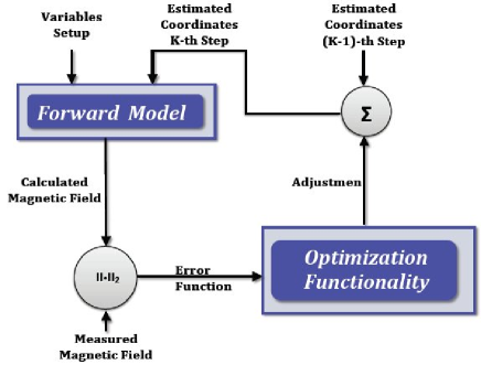
Figure 2: Blocks diagram of the inverse problem algorithm.

The unknown end-points segments coordinates s are obtained through an iterative procedure which, at each step, computes the correction factors needed to obtain the new set of coordinates. The correction factors are evaluated by the optimization functionality, on the basis of the difference in 2-norm between the measured fields and the fields computed by the forward solver. Since the problem is strictly nonlinear, the solver of the inverse problem was based on the Levenberg-Marquardt (LM) algorithm [15]. In brief, the LM algorithm starts from an initial set of reasonable end-points segments coordinates $s^{(0)}$: this set is then updated at each step k by adding the solutions $\Delta s^{(k)}$ of the linear system shown in equation (10)

$$\left(\tilde{\textbf{B}}^{(k)}+\beta^{(k)}\textit{diag}[\tilde{\textbf{B}}^{(k)}]\right)\Delta\textbf{s}^{(k)}=-\textbf{G}^{(k)^{T}}\textit{F}(\textbf{s}^{(k)})$$ (10)

In equation (10) the matrix $\tilde{\textbf{B}}^{(k)}$ is an approximation of the Hessian matrix of F at step k and is equal to $\textbf{G}^{(k)^{T}}$ $\textbf{G}^{(k)}$, with $\textbf{G}^{(k)}$ as the gradient of the error function F at step k, while $\beta^{(k)}$ is an adaptive parameter. Once $\Delta$ $\textbf{s}^{(k)}$ is known, the new coordinates are calculated by the following equation:

$$\textbf{s}^{(k+1)}=\textbf{s}^{(k)}+\Delta\textbf{s}^{(k)}$$ (11)

3 Numerical results

In order to validate the capabilities of the proposed method, some numerical experiments concerning the position estimation estimation of the antenna’s branches are carried out. The thin-wire antenna is assumed to be made by a nickel titanium thin wire 0.1 mm in radius, 2.1 cm in length with an electrical conductivity of $1.1\cdot{10^{6}}$ S/m. In this way the thin wire assumption is verified. The nickel-titanium alloy is selected because it is the most diffused alloy in the biomedical applications. It has to be underlined that this type of antenna can be effectively realized in practice and some of the human cavities may be investigated. Moreover, the number of branches for the antenna is set to $N_{b}=4$, with shape shown in figure 3 and figure 4 by the red dashed line with squared markers. The antenna is fed by a sinusoidal current source with frequency equal to 100 MHz, and amplitude spacing in the following set of values: 0.1 mA, 1 mA, 5 mA, 25 mA and 50 mA. It has to be underlined that all these current values as well as the selected frequency can be well tolerated by the human tissues.
The ground surface of the antenna lies on the $\textit{Y}-\textit{Z}$ plane as showed in figure 3 and figure 4, and the feed point is placed at a distance of 2 mm from the ground plane.

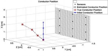
Figure 3: Conductor’s position estimated by flat sensor panel: the initial position is that a of straight thin-wire antenna 2.1 cm length, perpendicular to x = 0 plane.

Two sets of 12 sensors are considered. The sensors are assumed to be sensitive to the component along the Z axis of the magnetic field and placed on a flat surface in a first case study.
A semi-cylindrical surface sensors panel is then also considered (figure 4). The flat sensor panel is 3.5 cm height and 1.5 cm width, while the semi-cylindrical one has 1.5 cm radius and 3.5 cm height.

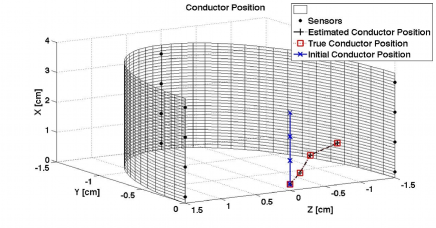
Figure 4: Conductor’s position estimated by semi-cylindrical sensor panel: the initial position is that of a straight thin-wire antenna 2.1 cm length, perpendicular to x = 0 plane.

For the above described set up, the measured values are calculated by means of the MoM based forward solver described in section 2. The initial set of end-points segments coordinates $s^{(0)}$ for the LM optimization algorithm is that of a straight thin-wire antenna 2.1 cm length and perpendicular to the ground plane. From these coordinates the true position of each branch is then estimated. Figure 3 shows the estimated position of the conductor in the case of the flat sensors panel. The picture shows that the distance between the estimated position, the black dashed line with plus markers, and the true position, the red dashed line with square markers, is close to zero.

Table 1: Relative error and number of iteration required with the flat sensors panel

Current [mA]	Relative error	No. of iterations
0.1	6.15e-11	169
1	6.10e-11	165
5	7.88e-09	87
25	3.78e-10	28
50	1.53e-11	8

For this configuration, Table 1 shows the 2-norm relative error between true and estimated coordinates values for a given level of current, and the number of iterations. The simulations results show that the error is close to zero, also for small values of the source current. This gives benefit for the future development of the antenna’s power system and a benefit for the patient. Figure 4 shows the estimated position of the conductor for the semi-cylindrical sensors panel.

Table 2: Relative error and number of iteration required with the semi-cylindrical sensors panel

Current [mA]	Relative error	No. of iterations
0.1	3.05e-10	25
1	1.04e-09	17
5	1.75e-11	12
25	2.55e-12	8
50	1.00e-09	8

The picture shows as the distance between the estimated position, the black dashed line with plus markers, and the true position, the red dashed line with square markers, is close to zero. For this scenario, the 2-norm relative error between true and estimated coordinates for a given level of source current, and the number of iterations are shown in Table 2. The simulations results show that the error is close to zero also in this case.

Note that a lower relative error has been reached for the flat sensors panel:this result can be justified because with the semi-cylindrical sensors panel the measured magnetic field components contain more information about the real field distribution. Moreover the number of iterations decreases as the source current amplitude increases for a same sensors configuration. However, the shape of the sensors panel influences also the convergence of the optimization algorithm: the semi-cylindrical sensors panel outperforms the flat sensors panel, especially for low levels of antenna source currents. This result suggests that the number of iterations can be reduced via a proper sensors panel design, without compromising the precision and without increasing the antenna currents, this latter aspect is fundamental for the invasiveness of the method.

4 Conclusions

In this paper, a numerical method to evaluate the shape of micro-structures for bio-medical application with a very low invasiveness for the human body, is proposed. A flexible thinwire antenna radiates the VHF waves and then, by numerically solving a typical inverse problem, the estimation of the antenna location enables to reconstruct the micro-structure’s image. The typical inverse problem is solved, and first simulation results assess the validity and the robustness of the proposed approach.

References

- [1] G. Ala, G. Di Blasi and E. Francomano, “A numerical meshless particle method in solving the magnetoencefalography forward problem,” International Journal of Numerical Modeling: Electronic Networks, Devices and Fields, vol. 25, no. 5-6, pp. 428–440, February 2012.
- [2] G. Ala, and E. Francomano, “A multi-sphere particle numerical model for non-invasive investigations of neuronal human brain activity”. method in solving the magnetoencefalography forward problem,” Progress In Electromagnetics Research Letters, vol. 36, pp. 143-153, 2013.
- [3] P. Di Barba, M.E. Mognaschi, G. Nolte, R. Palka and A. Savini, “Source identification based on regularization and evolutionary computing in biomagnetism,” COMPEL, vol. 29, no. 4, pp. 1022–1032, 2010.
- [4] A. Fhager, P. Hashemzadeh and M. Persson, “Reconstruction quality and spectral content of an electromagnetic time-domain inversion algorithm,” IEEE Transactions on Biomedical Engineering, vol. 53, no. 8, pp. 1594– 1604, August 2006.
- [5] R.D. Foster, D.A. Pistenmaa, T.D. Solberg, “A comparison of radiographic techniques and electromagnetic transponders for localization of the prostate,” Radiation Oncology, vol. 7, no. 1, 2012.
- [6] Z. Zakaria, R.A. Rahim, M.S.B. Mansor, S. Yaacob, N. M. N. Ayob, S.Z.M. Muji, M.H.F. Rahiman and S.M.K.S. Aman, “Advancements in transmitters and sensors for biological tissue imaging in Magnetic Induction Tomography,” Sensors (Switzerland), vol. 12, no. 6, pp. 7126– 7156, 2012.
- [7] T. Williams, J. Sill and E. Fear, “Breast surface estimation for radar based breast imaging systems,” IEEE Transactions on Biomedical Engineering, vol. 55, no. 6, pp. 1678–1686, June 2008.
- [8] D.B. Davidson, U. Jakobus and M.A. Stuchly, “Human exposure assessment in the near field of GSM base-station antennas using a hybrid finite element/method of moments technique,” IEEE Transactions on Biomedical Engineering, vol. 50, no. 2, pp. 224–233, February 2003.
- [9] G. Ala, P. Buccheri, E. Francomano, A. Tortorici, “Advanced algorithm for transient analysis of grounding systems by moments method,” in IEE Conference Publication, IEE, Ed., 1994, pp. 363–366.
- [10] G. Ala, E. Francomano and A. Tortorici, “Iterative moment method for electromagnetic transients in grounding systems on CRAY T3D,” Lecture Notes in Computer Science, vol. 1041, no. 1, pp. 9–16, August 1996.
- [11] G. Ala, E. Francomano and A. Tortorici,, “The method of moments for electromagnetic transients in grounding systems on distributed memory multiprocessors,” Parallel Algorithms and Applications, vol. 14, no. 3, pp. 213–233, 2000.
- [12] G. Ala and M.L. Di Silvestre, “A simulation model for electromagnetic transients in lightning protection systems,” IEEE Transactions on Electromagnetic Compatibility, vol. 44, no. 4, pp. 539–554, July 2002.
- [13] G. Ala, M.L. Di Silvestre, E. Francomano and A. Tortorici, “An advanced numerical model in solving thin-wire integral equations by using semi-orthogonal compactly supported spline wavelets,” IEEE Transactions on Electromagnetic Compatibility, vol. 45, no. 2, pp. 218– 228, May 2003.
- [14] G. Ala, M.L. Di Silvestre, E. Francomano and A. Tortorici, “Wavelet-based efficient simulation of electromagnetic transients in a lightning protection system,” IEEE Transactions on Magnetics, vol. 39, no. 3, pp. 1257–1260, 2003.
- [15] G. Ala, M.C. Di Piazza, G. Tine’, F. Viola and G. Vitale, “Evaluation of radiated EMI in 42 V vehicle electrical systems by FDTD simulation,” IEEE Transactions on Vehicular Technology, vol. 56, no. 4, pp. 1477– 1484, July 2007.
- [16] W.H. Press, S.A. Teukolsky, W.T. Vetterling and B.P. Flannery, Numerical recipes: the art of scientific computing. Cambridge: Cambridge University Press, 2007.
- [17] E. Francomano, A. Tortorici, C. Lodato and S. Lopes, “An algorithm for optical flow computation based on a quasi-interpolant operator,” Computing Letters, vol. 2, no. 1-2, pp. 93–106, May 2006.