RAMSES-RT: Radiation hydrodynamics in the cosmological context

Abstract

We present a new implementation of radiation hydrodynamics (RHD) in the adaptive mesh refinement (AMR) code RAMSES. The multi-group radiative transfer (RT) is performed on the AMR grid with a first-order Godunov method using the M1 closure for the Eddington tensor, and is coupled to the hydrodynamics via non-equilibrium thermochemistry of hydrogen and helium. This moment-based approach has the large advantage that the computational cost is independent of the number of radiative sources - it can even deal with continuous regions of emission such as bound-free emission from gas. As it is built directly into RAMSES, the RT takes natural advantage of the refinement and parallelization strategies already in place. Since we use an explicit advection solver for the radiative transport, the time step is restricted by the speed of light - a severe limitation that can be alleviated using the so–called “reduced speed of light” approximation. We propose a rigorous framework to assess the validity of this approximation in various conditions encountered in cosmology and galaxy formation. We finally perform with our newly developed code a complete suite of RHD tests, comparing our results to other RHD codes. The tests demonstrate that our code performs very well and is ideally suited for exploring the effect of radiation on current scenarios of structure and galaxy formation.

1 Introduction

With the surging interest in reionization and the first sources of light in the Universe, and also thanks to a steadily increasing computational power, cosmological simulation codes have begun to include ionizing radiative transfer (RT) in the last decade or so. This is generally seen as a second-order component in most astrophysical processes, but important nonetheless, and is obviously very important in the context of simulating reionization. Due to the challenges involved, most implementations have started out with the post-processing of ionizing radiation on simulations including only dark matter, but a few have begun doing coupled radiation hydrodynamics (RHD), which model the interplay of radiation and gas.

It is highly desirable to follow self-consistently, with RHD simulations, the time-evolution and morphology of large-scale intergalactic medium (IGM) reionization and at the same time the smaller scale formation of the presumed sources of reionization; how galaxy formation is regulated by the ionizing radiation being released, how much of the radiation escapes from the galaxies to ionize the IGM, how first generation stars are formed in a metal-free environment and how radiative and supernovae feedback from those stars affect the inter-galactic medium. The galaxies and the IGM are indeed inter-connected via the ionizing radiation: the photons released from the galaxies affect the state of the surrounding gas via ionization and heating and may even prevent it from falling in or condensing into external gravitational potentials, especially small ones (e.g. Wise & Abel, 2008; Ocvirk & Aubert, 2011), which can then in turn significantly alter the ionization history.

The importance of RT and RHD is of course not limited to the epoch of reionization. Stars keep emitting ionizing radiation after this epoch and their radiative feedback likely has an effect on the post-reionization regulation of star-formation (e.g. Pawlik & Schaye, 2009; Hopkins, Quataert & Murray, 2011), the mass distribution of stellar populations (Krumholz, Klein & McKee, 2012) and even gas outflows (Hopkins et al., 2012).

Radiation hydrodynamics are complex and costly in simulations. The inclusion of coupled radiative transfer in hydrodynamical codes in general is challenging mainly because of the high dimensionality of radiative transfer (space-, angular-, and frequency dimensions) and the inherent difference between the typical timescales of radiative transfer and non-relativistic hydrodynamics. Simulating the interaction between small and large scales (so relevant to the epoch of cosmic reionization) makes things even worse: one wants to simulate, in a statistically significant region of the Universe (i.e. of the order of 100 comoving Mpc across) the condensation of matter in galaxy groups on Mpc scales, down to individual galaxies on kpc scales, followed by the formations of stellar nurseries in those galaxies on pc scales, and ultimately the formation of stars on sub-pc scales and then the effect of radiation from those stars back to the large scale IGM. This cycle involves size differences of something like 9 to 10 orders of magnitude – which is too much for the most advanced codes and computers today, actually even so without the inclusion of radiative transfer.

Due to these challenges, simulations typically focus on only a subset of these scales; either they consider reionization on large scales and apply sub-resolution recipes to determine stellar luminosities and UV escape fractions, or they ignore the cosmological context and focus on star formation and escape fractions in isolated galaxies or even isolated stellar nurseries.

A number of large scale 3D radiative transfer simulations of reionization have been carried out in recent years (e.g. Gnedin & Ostriker, 1997; Miralda-Escudé, Haehnelt & Rees, 2000; Gnedin, 2000; Ciardi, Stoehr & White, 2003; Sokasian et al., 2004; Iliev et al., 2006b; Zahn et al., 2007; Croft & Altay, 2008; Baek et al., 2010; Aubert & Teyssier, 2010; Petkova & Springel, 2011b), though they must all to some degree use subgrid recipes for star formation rates, stellar luminosities and UV escape fractions, none of which are well constrained. The ionization history in these simulations thus largely depends on these input parameters and resolution – some in fact use the observational constraints of the ionization history to derive constraints on these free parameters (e.g. Sokasian et al., 2004; Croft & Altay, 2008; Baek et al., 2010; Aubert & Teyssier, 2010; Petkova & Springel, 2011b). Furthermore, most of these works have used a post-processing RT strategy instead of RHD, which neglects the effect the ionizing radiation has on the formation of luminous sources.

The primary driver behind this work is the desire to understand the birth of galaxies and stars during the dark ages, and how they link with their large scale environment. We have thus implemented a RHD version of the widely used cosmological code RAMSES (Teyssier, 2002), that we call RAMSES-RT, with the goal of running cosmological RHD simulations, optimized for galactic scale radiation hydrodynamics. RAMSES is an adaptive mesh refinement (AMR) code, which greatly cuts costs by adaptively allowing the resolution to follow the formation of structures. The RHD implementation takes full advantage of the AMR strategy, allowing for high resolution simulations that can self consistently model the interplay of the reionizing Universe and the formation of the first galaxies.

Some of the goals we will be able to tackle with this implementation are:

• Study radiative feedback effects in primordial galaxies. These galaxies are by definition young and small, and the first stars are thought to be gigantic and very bright due to the lack of metals. The ionizing radiation from these first stars is likely to have a dramatic effect on the galaxy evolution. This is closely associated with the formation of molecules, needed to form the first stars, which is sensitive to the radiation field. Radiative feedback effects also appear to be relevant in lower-redshift galaxies, and likely have a considerable impact on the initial mass function of stellar populations (Krumholz, Klein & McKee, 2012).

• Investigate the escape of ionizing photons from early galaxies, how it affects the ionization history and external structure formation, e.g. the formation of satellite galaxies.

• Study the emission and absorption properties of galaxies and extended structures. Observable properties of gas are highly dependent on its ionization state, which in turn depends on the local radiation field (e.g. Oppenheimer & Schaye, 2013). To predict it correctly, and to make correct interpretations of existing observations, one thus needs to model the ionization state consistently, for which RHD simulations are needed.

• Improve sub-resolution recipes: of course we have not implemented a miracle code, and we are still nowhere near simulating simultaneously the 9 to 10 orders of magnitude in scale needed for fully self-consistent simulations of reionization. Sub-resolution strategies are still needed, and part of the objective is to improve those via small-scale simulations of stellar feedback (SNe, radiation, stellar winds).

It is useful here to make clear the distinction between continuum and line radiative transfer: our goal is to study the interplay of ionizing radiation, e.g. from stellar populations and AGN, and the interstellar/intergalactic gas. We consider continuum radiation, because the spectra of stars (and AGN) are smooth enough that emission and absorption processes are not sensitive to subtle rest-frame frequency shifts, be they due to local gas velocities or cosmological expansion.

On the other side is line transfer, i.e. the propagation of radiation over a narrow frequency range, usually corresponding to a central frequency that resonates with the gas particles. An important example is the propagation of Ly$\alpha$ photons. Here, one is interested in the complex frequency and direction shifts that take place via scattering on the gas particles, and gas velocities and subtle frequency shifts are vital components. Line transfer is mostly done to interpret observational spectra, e.g. from Ly$\alpha$ emitting/absorbing galaxies (e.g. Verhamme, Schaerer & Maselli, 2006), and is usually run in post-processing under the assumption that the line radiation has a negligible effect on the gas dynamics (through this assumption is not neccessarily true; see Dijkstra & Loeb, 2009).

There is a bit of a grey line between those two regimes of continuum and line radiation - some codes are even able to do both (e.g. Baek et al., 2009; Pierleoni, Maselli & Ciardi, 2009; Yajima et al., 2012). Our implementation deals strictly with continuum radiation though, as do most RHD implementations, for the sake of speed and memory limitations. We do approximate multi-frequency, but only quite coarsely, such that simulated photons represent an average of photons over a relatively wide frequency range, and any subtle frequency shifts and velocity effects are ignored.

1.1 Radiative transfer schemes and existing implementations

Cosmological hydrodynamics codes have traditionally been divided into two categories: Smoothed Particle Hydrodynamics (SPH) and AMR. The drawbacks and advantages of each method have been thoroughly explored (e.g. Agertz et al., 2007; Wadsley, Veeravalli & Couchman, 2008; Tasker et al., 2008) and we now believe that both code types agree more or less on the final result if they are used carefully with recently developed fixes and improvements, and if applied in their regimes of validity. On the radiation side, it is quite remarkable that we have the same dichotomy between ray-tracing codes and moment-based codes. Comparative evaluations of both methods have been performed in several papers (Iliev et al., 2006a; Altay, Croft & Pelupessy, 2008; Aubert & Teyssier, 2008; Pawlik & Schaye, 2008; Iliev et al., 2009; Maselli, Ciardi & Kanekar, 2009; Petkova & Springel, 2009; Cantalupo & Porciani, 2011; Pawlik & Schaye, 2011; Petkova & Springel, 2011a; Wise & Abel, 2011), and here again, each method has its own specific advantage over the other one. Comparing both methods in the coupled case (RHD) within the more challenging context of galaxy formation, such as in the recent Aquila comparison project, (Scannapieco et al., 2012), remains to be done.

1.1.1 Ray-based schemes

Here the approximation is made that the radiation field is dominated by a limited number of sources. This allows one to approximate the local intensity of radiation, $I_{\nu}$, as a function of the optical depth $\tau$ along rays from each source.

The simplest solution is to cast rays, or long characteristics from each source to each cell (or volume element) and sum up the optical depth at each endpoint. With the optical depths in hand, $I_{\nu}$ is known everywhere and the rates of photoionization, heating and cooling can be calculated. While this strategy has the advantage of being simple and easy to parallelize (each source calculation is independent from the other), there is a lot of redundancy, since any cell which is close to a radiative source is traversed by many rays cast to further-lying cells, and is thus queried many times for its contribution to the optical depth. The parallelization is also not really so advantageous in the case of multiprocessor codes, since rays that travel over large lengths likely need to access cell states over many CPU nodes, calling for a lot of inter-node communication. Furthermore, the method is expensive: the computational cost scales linearly with the number of radiative sources, and each RT timestep has order $\mathcal{O}(N_{\rm{sources}}\ N_{\rm{cells}})$ operations, where $N_{\rm{sources}}$ is the number of radiative sources and $N_{\rm{cells}}$ is the number of volume elements. Implementation examples include Abel, Norman & Madau (1999), Cen (2002) and Susa (2006).

Short characteristics schemes overcome the redundancy problem by not casting separate rays for each destination cell. Instead, the calculation of optical depths in cells is propagated outwards from the source, and is in each cell based on the entering optical depths from the inner-lying cells. Calculation of the optical depth in a cell thus requires some sort of interpolation from the inner ones. There is no redundancy, as only a single ray segment is cast through each cell in one time-step. However, there is still a large number of operations and the problem has been made inherently serial, since the optical depths must be calculated in a sequence which follows the radiation ripple away from the source. Some examples are Nakamoto, Umemura & Susa (2001), Mellema et al. (2006), Whalen & Norman (2006) and Alvarez, Bromm & Shapiro (2006).

Adaptive ray tracing (e.g. Abel & Wandelt, 2002; Razoumov & Cardall, 2005; Wise & Abel, 2011) is a variant on long characteristics, where rays of photons are integrated outwards from the source, updating the ray at every step of the way via absorption. To minimize redundancy, only a handful of rays are cast from the source, but they are split into sub-rays to ensure that all cells are covered by them, and they can be merged again if need be.

Cones are a variant on short characteristics, used in conjunction with SPH (Pawlik & Schaye, 2008, 2011) and the moving-mesh AREPO code (Petkova & Springel, 2011a). The angular dimension of the RT equation is discretized into tesselating cones that can collect radiation from multiple sources and thus ease the computational load and even allow for the inclusion of continuous sources, e.g. gas collisional recombination.

A hybrid method proposed by Rijkhorst et al. (2006) combines the long and short characteristics on patch-based grids (like AMR), to get rid of most of the redundancy while keeping the parallel nature. Long characteristics are used inside patches, while short characteristics are used for the inter-patches calculations.

Monte-Carlo schemes do without splitting or merging of rays, but instead reduce the computational cost by sampling the radiation field, typically both in the angular and frequency dimensions, into photon packets that are emitted and traced away from the source. The cost can thus be adjusted with the number of packets emitted, but generally this number must be high in order to minimize the noise inherent to such a statistical method. Examples include Ciardi et al. (2001), Maselli, Ferrara & Ciardi (2003), Altay, Croft & Pelupessy (2008), Baek et al. (2009), and Cantalupo & Porciani (2011). An advantage of the Monte-Carlo approach of tracking individual photon packets is that it naturally allows for keeping track of the scattering of photons. For line radiation transfer, where doppler/redshift effects in resonant photon scattering are important, Monte-Carlo schemes are the only feasible way to go – though in these cases, post-processing RT is usually sufficient (e.g. Cantalupo et al., 2005; Verhamme, Schaerer & Maselli, 2006; Laursen & Sommer-Larsen, 2007; Pierleoni, Maselli & Ciardi, 2009).

Ray-based schemes in general assume infinite light speed, i.e. rays are cast from source to destination instantaneously. Many authors note that this only affects the initial speed of ionization fronts (I-fronts) around points sources (being faster than the light speed), but it may also result in an over-estimated I-front speed in underdense regions (see §6.5), and may thus give incorrect results in reionization experiments where voids are re-ionized too quickly. Some ray schemes (e.g. Pawlik & Schaye, 2008; Petkova & Springel, 2011a; Wise & Abel, 2011) allow for finite light speed, but this adds to the complexity, memory requirement and computational load. With the exception of the cone-based methods (and to some degree the Wise & Abel (2011) implementation), which can combine radiation from many sources into single rays, ray-based schemes share the disadvantage that the computational load increases linearly with the number of radiative sources. Moment methods can naturally tackle this problem, though other limitations appear instead.

1.1.2 Moment-based radiative transfer

An alternative to ray-tracing schemes is to reduce the angular dimensions by taking angular moments of the RT equation (Eq. 2). Intuitively this can be thought of as switching from a beam description to that of a field or a fluid, where the individual beams are replaced with a “bulk” direction that represents an average of all the photons crossing a given volume element in space. This infers useful simplifications: two angular dimensions are eliminated from the problem, and the equations take a form of conservation laws, like the Euler equations of hydrodynamics. They are thus rather easily coupled to these equations, and can be solved with numerical methods designed for hydrodynamics. Since radiation is not tracked individually from each source, but rather just added to the radiation field, the computation load is naturally independent of the number of sources.

The main advantage is also the main drawback: the directionality is largely lost in the moment approximation and the radiation becomes somewhat diffusive, which is generally a good description in the optically thick limit, where the radiation scatters a lot, but not in the optically thin regime where the radiation is free-streaming. Radiation has a tendency to creep around corners with moment methods. Shadows are usually only coarsely approximated, if at all, though we will see e.g. in section §6.4 that sharp shadows can be maintained with idealized setups and a specific solver.

The large value of the speed of light is also an issue. Moment methods based on an explicit time marching scheme have to follow a Courant stability condition that basically limits the radiation from crossing more than one volume element in one time-step. This requires to perform many time-steps to simulate a light crossing time in the free-streaming limit, or, as we will see later, to reduce artificially the light speed. Implicit solvers can somewhat alleviate this limitation, at the price of inverting large sparse matrices which are usually ill-conditioned and require expensive, poorly parallelized, relaxation methods.

The frequency dimension is also reduced, via integration over frequency bins: in the grey (single group) approximation the integral is performed over the whole relevant frequency range, typically from the hydrogen ionization frequency and upwards. In the multigroup approximation, the frequency range is split into a handful of bins, or photon groups, (rarely more than a few tens due to memory and computational limitations) and the equations of radiative transfer can be solved separately for each group. Ray-tracing schemes also often discretize into some number of frequency bins, and they are usually more flexible in this regard than moment-based schemes: while the spectrum of each source can be discretized individually in ray-tracing, the discretization is fixed in space in moment-based schemes, i.e. the frequency intervals and resulting averaged photon properties must be the same everywhere, due to the field approximation.

In the simplest form of moment-based RT implementations, so-called flux limited diffusion (FLD), only the zero-th order moment of the radiative transfer equation is used, resulting in an elliptic set of conservation laws. A closure is provided in the form of a local diffusion relation, which lets the radiation flow in the direction of decreasing gas internal energy (i.e. in the direction opposite of the energy gradient). This is realistic only if the medium is optically thick, and shadows cannot be modelled. The FLD method has been used by e.g. Krumholz et al. (2007), Reynolds et al. (2009) and Commerçon et al. (2011), mainly for the purpose of studying the momentum feedback of infrared radiation onto dusty and optically thick gas, rather than photoionization of hydrogen and helium.

Gnedin & Abel (2001) and Petkova & Springel (2009) used the optically thin variable Eddington tensor formalism (OTVET), in which the direction of the radiative field is composed on-the-fly in every point in space from all the radiative sources in the simulation, assuming that the medium between source and destination is transparent (hence optically thin). This calculation is pretty fast, given the number of relevant radiative sources is not overburdening, and one can neglect these in-between gas cells. Finlator, Özel & Davé (2009) take this further and include in the calculation the optical thickness between source and destination with a long characteristics method, which makes for an accurate but slow implementation. A clear disadvantage here is that in using the radiation sources to close the moment equations and compute the flux direction, the scaling of the computational load with the number of sources is re-introduced, hence negating one of the main advantages of moment-based RT.

González, Audit & Huynh (2007), AT08 and Vaytet, Audit & Dubroca (2010) – and now us – use a different closure formalism, the so-called M1 closure, which can establish and retain bulk directionality of photon flows, and can to some degree model shadows behind opaque obstacles. The M1 closure is very advantageous in the sense that it is purely local, i.e. it requires no information which lies outside the cell, which is not the case for the OTVET approximation.

As shown by Dubroca & Feugeas (1999), the M1 closure has the further advantage that it makes the system of RT equations take locally the form of a hyperbolic system of conservations laws, where the characteristic wave speeds can be calculated explicitly and are usually close, but always smaller than the speed of light $c$. Hyperbolic systems of conservation laws are mathematically well understood and thoroughly investigated, and a plethora of numerical methods exist to deal with them (e.g. Toro, 1999). In fact, the Euler equations are also a hyperbolic system of conservation laws, which implies we have the RT equations in a form which is well suited to lie alongside existing hydrodynamical solvers, e.g. in RAMSES.

1.2 From ATON to RAMSES-RT

The ATON code (AT08, Aubert & Teyssier, 2010) uses graphical processing units, or GPUs, to post-process the transfer of monochromatic photons and their interaction with hydrogen gas. GPUs are very fast, and therefore offer the possibility to use the correct (very large) value for the speed of light and perform hundreds to thousands of radiation sub-cycles at a reasonable cost, but only if the data is optimally structured in memory, such that volume elements that are close in space are also close in memory. It is ideal for post-processing RT on simulation outputs that are projected onto a Cartesian grid, but hard to couple directly with an AMR grid in order to play an active part in any complex galaxy formation simulation. Even so, we have in the newest version of the ATON code included the possibility to perform fully coupled RHD simulations using a Cartesian grid only (this usually corresponds to our coarser grid level in the AMR hierarchy), where RT is performed using the ATON module on GPUs.

In our RAMSES-RT implementation we use the same RT method as ATON does – the moment method with the M1 Eddington tensor closure. The biggest difference is that RAMSES-RT is built directly into the RAMSES cosmological hydrodynamics code, allowing us to perform RHD simulations directly on the AMR grid, without any transfer of data between different grid structures. Furthermore, we have expanded the implementation to include multigroup photons to approximate multifrequency, and we have added the interactions between photons and helium. We explicitly store and advect the ionization states of hydrogen and helium, and we have built into RAMSES-RT a new non-equilibrium thermochemistry model that evolves these states along with the temperature and the radiation field through chemical processes, photon absorption and emission. Finally, for realistic radiative feedback from stellar populations, we have enabled RAMSES-RT to read external spectral energy distribution (SED) models and derive from them luminosities and UV “colors” of simulated stellar sources.

We have already listed a number of RT implementations, two of which even function already in the RAMSES code (AT08, Commerçon et al., 2011), and one might ask whether another one is really needed. To first answer for the ATON implementation, it is optimized for a different regime than RAMSES-RT. As discussed, ATON prefers to work with structured grids, but it cannot deal well with adaptive refinement. This, plus the speed of ATON, makes it very good for studying large scale cosmological reionization, but not good for AMR simulations of individual halos/galaxies, e.g. cosmological zoom simulations, where the subject of interest is the effect of radiative feedback on the formation of structures and galaxy evolution, and escape fractions of ionizing radiation. The Commerçon et al. (2011) implementation is on the opposite side of the spectrum. Being based on the FLD method, it is optimized for RHD simulations of optically thick protostellar gas. It is a monogroup code that doesn’t track the ionization state of the gas. Furthermore, it uses a rather costly implicit solver, which makes it hard to adapt to multiple adaptive time stepping usually used in galaxy formation problems.

A few codes have been used for published 3D cosmological RHD simulations with ionizing radiation. As far as we can see these are Gnedin (2000), Kohler, Gnedin & Hamilton (2007) (both in $\tt SLH-P^{3}M$), Shin, Trac & Cen (2008), Petkova & Springel (2009) (in GADGET), Wise & Abel (2011) (in ENZO), Finlator, Dave & Ozel (2011) (in GADGET), Hasegawa & Semelin (2013) (START), and Pawlik, Milosavljević & Bromm (2013) (in GADGET). A few others that have been used for published astrophysical (ionizing) RHD simulations but without a co-evolving cosmology are Mellema et al. (2006), Susa (2006), Whalen & Norman (2006), and Baek et al. (2009). The rest apparently only do post-processing RT, aren’t parallel or are otherwise not efficient enough. Many of these codes are also optimized for cosmological reionization rather than galaxy-scale feedback.

Thus there aren’t so many cosmological RHD implementations out there, and there should be room for more. The main advantage of our implementation is that our method allows for an unlimited number of radiative sources and can even easily handle continuous sources, and is thus ideal for modelling e.g. the effects of radiative feedback in highly resolved simulations of galaxy formation, UV escape fractions, and the effects of self-shielding on the emission properties of gas and structure formation, e.g. in the context of galaxy formation in weak gravitational potentials.

The structure of the paper is as follows: in §2 we present the moment based RT method we use. In §3 we explain how we inject and transport radiation on a grid of gas cells, and how we calculate the thermochemistry in each cell, that incorporates the absorption and emission of radiation. In §4 we present two tricks we use to speed up the RHD code, namely to reduce the speed of light, and to “smooth” out the effect of operator splitting. In §5 we describe how the radiative transfer calculation is placed in the numerical scheme of RAMSES, and demonstrate that the radiation is accurately transported across an AMR grid. In §6, we present our test suite, demonstrating that our code performs very well in coupled radiation hydrodynamics problems and finally, §7 summarizes this work and points towards features that may be added in the future. Details of the thermochemistry and additional code tests are described in the appendix.

2 Moment-based radiative transfer with the M1 closure

Let $I_{\nu}({\bf{x}},{\bf{n}},t)$ denote the radiation specific intensity at location ${\bf{x}}$ and time $t$, such that

$$I_{\nu}\ d\nu\ d\Omega\ dA\ dt$$ (1)

is the energy of photons with frequency over the range $d\nu$ around $\nu$ propagating through the area $dA$ in a solid angle $d\Omega$ around the direction ${\bf{n}}$.

The equation of radiative transfer (e.g. Mihalas & Mihalas, 1984) describes the local change in $I_{\nu}$ as a function of propagation, absorption and emission,

$$\frac{1}{c}\frac{\partial I_{\nu}}{\partial t}+{\bf{n}}\cdot\nabla I_{\nu}=-\kappa_{\nu}I_{\nu}+\eta_{\nu},$$ (2)

where $c$ is the speed of light, $\kappa_{\nu}({\bf{x}},{\bf{n}},t)$ is an absorption coefficient and $\eta_{\nu}({\bf{x}},{\bf{n}},t)$ a source function.

By taking the zeroth and first angular moments of (2), we can derive the moment-based RT equations that describe the time-evolution of photon number density $N_{\nu}$ and flux ${\bf{F}}_{\nu}$ (see e.g. AT08):

$$\frac{\partial N_{\nu}}{\partial t}+\nabla\cdot{\bf{F}}_{\nu} =-\sum_{j}^{{\rm{H\textsc{i}}},{\rm{He\textsc{i}}},\rm{He\textsc{ii}}}{n_{j}\sigma_{\nu j}cN_{\nu}}+{\dot{N}}^{\star}_{\nu}+{\dot{N}}^{rec}_{\nu}$$ (3)

$$\frac{\partial{\bf{F}}_{\nu}}{\partial t}+{c^{2}}\nabla\cdot{\bf{\mathds{P}}}_{\nu} =-\sum_{j}^{{\rm{H\textsc{i}}},{\rm{He\textsc{i}}},\rm{He\textsc{ii}}}{n_{j}\sigma_{\nu j}c{\bf{F}}_{\nu}},$$ (4)

where ${\bf{\mathds{P}}}_{\nu}$ is the radiative pressure tensor that remains to be determined to close the set of equations. Here we have split the absorption coefficient into constituent terms, $n_{j}\sigma_{\nu j}$, where $n_{j}$ is number density of the photo-absorbing species $j$ (=Hi, Hei, Heii), and $\sigma_{\nu j}$ is the ionization cross section between $\nu$-frequency photons and species $j$. Furthermore we have split the source function into (e.g. stellar, quasar) injection sources, ${\dot{N}}^{\star}_{\nu}$, and recombination radiation from gas, ${\dot{N}}^{rec}_{\nu}$. Here we only consider the photo-absorption of hydrogen and helium, which is obviously most relevant in the regime of UV photons. However, other absorbers can straightforwardly be added to the system.

Eqs. (3)-(4) are continuous in $\nu$, and they must be discretized to be usable in a numerical code. AT08 collected all relevant frequencies into one bin, so the equations could be solved for one group of photons whose attributes represent averages over the frequency range. For a rough approximation of multifrequency, we split the relevant frequency range into a number of photon groups, defined by

$$N_{i}=\int_{{\nu_{i\scriptscriptstyle 0}}}^{{\nu_{i\scriptscriptstyle 1}}}{N_{\nu}\;d\nu},\ \ \ \ \ \ \ \ \ {\bf{F}}_{i}=\int_{{\nu_{i\scriptscriptstyle 0}}}^{{\nu_{i\scriptscriptstyle 1}}}{{\bf{F}}_{\nu}\;d\nu},$$ (5)

where $({\nu_{i\scriptscriptstyle 0}},{\nu_{i\scriptscriptstyle 1}})$ is the frequency interval for group $i$. In the limit of one photon group, the frequency range is $({\nu_{i\scriptscriptstyle 0}},{\nu_{i\scriptscriptstyle 1}})=(\nu_{{\rm{H\textsc{i}}}},\infty)$; with $M>1$ groups, the frequency intervals should typically be mutually exclusive and set up to cover the whole H-ionizing range:

$$[\nu_{00},\nu_{01}:\nu_{10},\nu_{11}:...:\nu_{M0},\nu_{M1}]=[\nu_{{\rm{H\textsc{i}}}},\infty[.$$

Integrating the RT equations (3) and (4) over each frequency bin corresponding to the group definitions yields $M$ sets of four equations:

$$\frac{\partial N_{i}}{\partial t}+\nabla\cdot{\bf{F}}_{i} =-\sum_{j}^{{\rm{H\textsc{i}}},{\rm{He\textsc{i}}},\rm{He\textsc{ii}}}{n_{j}c{\sigma}^{\rm{N}}_{ij}N_{i}}\ \ +{\dot{N}}^{\star}_{i}+{\dot{N}}^{rec}_{i},$$ (6)

$$\frac{\partial{\bf{F}}_{i}}{\partial t}+{c^{2}}\nabla\cdot{\bf{\mathds{P}}}_{i} =-\sum_{j}^{{\rm{H\textsc{i}}},{\rm{He\textsc{i}}},\rm{He\textsc{ii}}}{n_{j}c{\sigma}^{\rm{N}}_{ij}{\bf{F}}_{i}},$$ (7)

where ${\sigma}^{\rm{N}}_{ij}$ represent average cross sections between each group $i$ and species $j$, defined by

$${\sigma}^{\rm{N}}_{ij}=\frac{\int_{{\nu_{i\scriptscriptstyle 0}}}^{{\nu_{i\scriptscriptstyle 1}}}{\sigma_{\nu j}N_{\nu}\ d\nu}}{\int_{{\nu_{i\scriptscriptstyle 0}}}^{{\nu_{i\scriptscriptstyle 1}}}{N_{\nu}\ d\nu}}.$$ (8)

We simplify things however by defining the group cross sections as global quantities, assuming a frequency distribution of energy $J(\nu)$ for the radiative sources (e.g. a black-body or some sophisticated model). The cross sections are thus in practice evaluated by

$${\sigma}^{\rm{N}}_{ij}=\frac{\int_{{\nu_{i\scriptscriptstyle 0}}}^{{\nu_{i\scriptscriptstyle 1}}}{\sigma_{\nu j}J(\nu)/h\nu\ d\nu}}{\int_{{\nu_{i\scriptscriptstyle 0}}}^{{\nu_{i\scriptscriptstyle 1}}}{J(\nu)/h\nu\ d\nu}},$$ (9)

where $h\nu$ is photon energy (with $h$ the Planck constant). Likewise, average photon energies within each group are evaluated by

$$\bar{\epsilon}_{i}=\frac{\int_{{\nu_{i\scriptscriptstyle 0}}}^{{\nu_{i\scriptscriptstyle 1}}}{J(\nu)\ d\nu}}{\int_{{\nu_{i\scriptscriptstyle 0}}}^{{\nu_{i\scriptscriptstyle 1}}}{J(\nu)/h\nu\ d\nu}},$$ (10)

and furthermore, for the calculation of photoionization heating, energy weighted cross sections are stored for each group - absorbing species couple:

$${\sigma}^{\rm{E}}_{ij}=\frac{\int_{{\nu_{i\scriptscriptstyle 0}}}^{{\nu_{i\scriptscriptstyle 1}}}{\sigma_{\nu j}J(\nu)\ d\nu}}{\int_{{\nu_{i\scriptscriptstyle 0}}}^{{\nu_{i\scriptscriptstyle 1}}}{J(\nu)\ d\nu}}.$$ (11)

In RAMSES-RT, ${\sigma}^{\rm{N}}_{ij}$, ${\sigma}^{\rm{E}}_{ij}$ and $\bar{\epsilon}_{i}$ can be either set by hand or evaluated on-the-fly from spectral energy distribution tables as luminosity weighted averages from in-simulation stellar populations, using the expressions from Verner et al. (1996) for $\sigma_{\nu,{\rm{H\textsc{i}}}}$, $\sigma_{\nu,{\rm{He\textsc{i}}}}$ and $\sigma_{\nu,\rm{He\textsc{ii}}}$.

For each photon group, the corresponding set of equations (6)-(7) must be closed with an expression for the pressure tensor ${\bf{\mathds{P}}}$. This tensor is usually described as the product of the photon number density and the so-called Eddington tensor ${\bf{\mathds{D}}}$ (see Eq. 12), for which some meaningful and physical expression is desired. Some formalisms have been suggested for ${\bf{\mathds{D}}}_{\nu}$. Gnedin & Abel (2001), Finlator, Özel & Davé (2009), and Petkova & Springel (2009) have used the so called optically thin Eddington tensor formalism (OTVET), in which ${\bf{\mathds{P}}}$ is composed on-the-fly from all the radiation sources, the main drawback being the computational cost associated with collecting the positions of every radiative source relative to every volume element. Instead, like AT08 (and González, Audit & Huynh 2007 before them), we use the M1 closure relation (Levermore, 1984), which has the great advantages that it is purely local, i.e. evaluating it in a piece of space only requires local quantities, and that it can retain a directionality along the flow of the radiative field. In our frequency-discretized form, the pressure tensor is given in each volume element for each photon group by

$${\bf{\mathds{P}}}_{i}={\bf{\mathds{D}}}_{i}N_{i}$$ (12)

where the Eddington tensor is

$${\bf{\mathds{D}}}_{i}=\frac{1-\chi_{i}}{2}\mathbf{I}+\frac{3\chi_{i}-1}{2}{\bf{n}}_{i}\otimes{\bf{n}}_{i}$$ (13)

and

$${\bf{n}}_{i}=\frac{{\bf{F}}_{i}}{|{\bf{F}}_{i}|},\ \ \ \ \ \chi_{i}=\frac{3+4f_{i}^{2}}{5+2\sqrt{4-3f_{i}^{2}}},\ \ \ \ \ f_{i}=\frac{|{\bf{F}}_{i}|}{cN_{i}},$$ (14)

are the unit vector pointing in the flux direction, the Eddington factor and the reduced flux, respectively. The reduced flux describes the directionality of the group $i$ radiation in each point, and must always have $0\leq f_{i}\leq 1$. A low value means the radiation is predominantly isotropic, and a high value means it is predominantly flowing in one direction. Photons injected into a point (via an increase in photon density only) initially have zero reduced flux and thus are isotropic. Away from the source, the moment equations and M1 closure develop a preferred outwards direction, i.e. the reduced flux tends towards one. Beams can be injected by imposing unity reduced flux on the injected photons. In this case, the M1 closure correctly maintains unity reduced flux (and $\chi=1$) along the beam (see demonstrations in Fig. 1 and Sections 5.3, 6.4, and 6.8). For the arguments leading to these expressions and a general discussion we point the reader towards Levermore (1984) and González, Audit & Huynh (2007) and AT08.

3 The radiative transfer implementation

We will now describe how pure radiative transfer is solved on a grid – without yet taking into consideration the hydrodynamical coupling. The details here are not very specific to RAMSES-RT and are much like those of AT08.

In addition to the usual hydrodynamical variables stored in every grid cell in RAMSES (gas density $\rho$, momentum density $\rho\bf{u}$, energy density $E$, metallicity $Z$), RAMSES-RT has the following variables: First, we have the $4\times M$ variables describing photon densities $N_{i}$ and fluxes ${\bf{F}}_{i}$ for the $M$ photon groups. Second, in order to consistently treat the interactions of photons and gas, we track the non-equilibrium evolution of hydrogen and helium ionization in every cell, stored in the form of passive scalars which are advected with the gas, namely

$$x_{\rm{H\scriptscriptstyle II}}=\frac{n_{\rm{H\scriptscriptstyle II}}}{n_{\rm{H}}},\ \ \ \ \ x_{\rm{He\scriptscriptstyle II}}=\frac{n_{\rm{He\scriptscriptstyle II}}}{n_{\rm{He}}},\ \ \ \ \ x_{\rm{He\scriptscriptstyle III}}=\frac{n_{\rm{He\scriptscriptstyle III}}}{n_{\rm{He}}}.$$ (15)

For each photon group, we solve the set of equations (6)-(7) with an operator splitting strategy, which involves decomposing the equations into three steps that are executed in sequence over the same time-step $\Delta t$, which has some pre-determined length. The steps are:

1. Photon injection step, where radiation from stellar and other radiative sources (other than gas recombinations) is injected into the grid. This corresponds to the ${\dot{N}}^{\star}_{i}$ term in (6).

2. Photon transport step, where photons are propagated in space. This corresponds to solving (6)-(7) with the RHS being equal to zero.

3. Thermochemistry step, where the rest of the RHS of (6)-(7) is solved. This is where the photons and the gas couple, so here we evolve not only the photon densities and fluxes, but also the ionization state and temperature of the gas.

3.1 The injection step

The equations to solve in this step are very simple,

$$\frac{\partial N_{i}}{\partial t}={\dot{N}}^{\star}_{i},$$ (16)

where ${\dot{N}}^{\star}_{i}$ is a rate of photon injection into photon group $i$, in the given cell. Normally, the injected photons come from stellar sources, but they could also include other point sources such as AGN, and also pre-defined point sources or even continuous “volume” sources.

Given the time $t$ and time-step length $\Delta t$, the discrete update in each cell done for each photon group is the following sum over all stellar particles situated in the cell:

$$N^{n+1}_{i} =N^{n}_{i}$$ (17)

$$+\frac{f_{\rm{esc}}}{V}\sum^{\rm{cell\ stars}}_{\star}m_{\star}\left[\Pi_{i}({\tau_{\star}}^{n+1},Z_{\star})-\Pi_{i}({\tau_{\star}}^{n},Z_{\star})\right],$$

where $n$ denotes the time index ($n=t$ and $n+1=t+\Delta t$), $f_{\rm{esc}}$ is an escape fraction, $V$ is the cell volume, $m_{\star}$, ${\tau_{\star}}$ and $Z_{\star}$ are mass, age and metallicity of the stellar particles, respectively, and $\Pi_{i}$ is some model for the accumulated number of group $i$ photons emitted per solar mass over the lifetime (so far) of a stellar particle. The escape fraction, $f_{\rm{esc}}$ is just a parameter that can be used to express the suppression (or even boosting) of radiation from processes that are unresolved inside the gas cell.

RAMSES-RT can read stellar energy distribution (SED) model tables to do on-the-fly evaluation of the stellar particle luminosities, $\Pi_{i}$. Photon cross sections and energies can also be determined on-the-fly from the same tables, to represent luminosity-weighted averages of the stellar populations in a simulation. Details are given in Appendix B.

3.2 The transport step

The equations describing free-flowing photons are

$$\frac{\partial N}{\partial t}+\nabla\cdot{\bf{F}}=0,$$ (18)

$$\frac{\partial{\bf{F}}}{\partial t}+c^{2}\nabla\cdot{\bf{\mathds{P}}}=0,$$ (19)

i.e. (6)-(7) with the RHS $=0$. Note that we have removed the photon group subscript, since this set of equations is solved independently for each group over the time-step.

(a)

(b)

(c)

(d)

(e)

(f)

(g)

(h)

Figure 1: Comparison of radiative transport in 2D RAMSES-RT runs (no photon-gas interaction) with the HLL (top) and GLF (bottom) flux functions, using isotropic point sources and beams. The box width in all runs is $1$ cm and the resolution is $256^{2}$ cells. For each isotropic point source, $10^{10}$ photons $\rm{s}^{-1}$ are injected continuously, and for each beam a constant photon density of $N=1\ {\rm{cm}}^{-2}$, with a unity reduced flux, is imposed on a region of one cell width and eight cell heights at the beam origin. The snapshots are taken at $t=5.2\times 10^{-11}$ s (a bit less than two light crossing times, long enough that a static configuration has been reached). Far left frames show single isotropic point sources. Middle left frames show attempts at creating horizontal and diagonal beams (with ${\bf{F}}=(cN,0)$ and ${\bf{F}}=(cN,cN)/\sqrt{2}$, respectively). Middle right frames show two isotropic point sources and how the photons behave between them. Far right frames show two beams of opposing directions and how a spurious weak perpendicular radiation source forms where they meet.

We can write the above equations in vector form

$$\frac{\partial{\mathcal{U}}}{\partial t}+\nabla{\mathcal{F}}({\mathcal{U}})=0,$$ (20)

where ${\mathcal{U}}=[N,{\bf{F}}]$ and ${\mathcal{F}}({\mathcal{U}})=[{\bf{F}},c^{2}{\bf{\mathds{P}}}]$. To solve (20) over time-step $\Delta t$, we use an explicit conservative formulation, expressed here in 1D for simplicity,

$$\frac{{\mathcal{U}}_{l}^{n+1}-{\mathcal{U}}_{l}^{n}}{\Delta t}+\frac{{\mathcal{F}}_{l+1/2}^{n}-{\mathcal{F}}_{l-1/2}^{n}}{\Delta x}=0,$$ (21)

where $n$ again denotes time index and $l$ denotes cell index along the x-axis. ${\mathcal{F}}_{l+1/2}$ and ${\mathcal{F}}_{l-1/2}={\mathcal{F}}_{(l-1)+1/2}$ are intercell fluxes evaluated at the cell interfaces. Simple algebra gives us the updated cell state,

$${\mathcal{U}}_{l}^{n+1}={\mathcal{U}}_{l}^{n}+\frac{\Delta t}{\Delta x}\left({\mathcal{F}}_{l-1/2}^{n}-{\mathcal{F}}_{l+1/2}^{n}\right),$$ (22)

and all we have to do is determine expressions for the intercell fluxes.

Many intercell flux functions are available for differential equations of the form (20) which give stable results in the form of (22) (see e.g. Toro, 1999), as long as the Courant time-step condition is respected (see §4.1). Following AT08 and González, Audit & Huynh (2007) we implement two flux functions which can be used in RAMSES-RT.

One is the Harten-Lax-van Leer (HLL) flux function (Harten, Lax & Leer, 1983),

$$\left({\mathcal{F}}_{\rm{HLL}}\right)_{l+1/2}^{n}=\frac{\lambda^{+}{\mathcal{F}}_{l}^{n}-\lambda^{-}{\mathcal{F}}_{l+1}^{n}+\lambda^{+}\lambda^{-}\left({\mathcal{U}}_{l+1}^{n}-{\mathcal{U}}_{l}^{n}\right)}{\lambda^{+}-\lambda^{-}},$$ (23)

where

$$\lambda^{+} =\max(0,\lambda^{\rm{max}}_{l},\lambda^{\rm{max}}_{l+1}),$$

$$\lambda^{-} =\min(0,\lambda^{\rm{min}}_{l},\lambda^{\rm{min}}_{l+1})$$

are maximum and minimum eigenvalues of the Jacobian $\partial{\mathcal{F}}/\partial{\mathcal{U}}$. These eigenvalues mathematically correspond to wave speeds, which in the case of 3D radiative transfer depend only on the magnitude of the reduced flux $f$ (14) and the angle of incidence of the flux vector to the cell interface. This dependence has been calculated and tabulated by González, Audit & Huynh (2007), and we use their table to extract the eigenvalues.

The other flux function we have implemented is the simpler Global Lax Friedrich (GLF) function,

$$\left({\mathcal{F}}_{\rm{GLF}}\right)_{l+1/2}^{n}=\frac{{\mathcal{F}}_{l}^{n}+{\mathcal{F}}_{l+1}^{n}}{2}-\frac{c}{2}\left({\mathcal{U}}_{l+1}^{n}-{\mathcal{U}}_{l}^{n}\right),$$ (24)

which corresponds to setting the HLL eigenvalues to the speed of light, i.e. $\lambda^{-}=-c$ and $\lambda^{+}=c$, and has the effect of making the radiative transport more diffusive. Beams and shadows are therefore better modelled with the HLL flux function than with the GLF one, whereas the inherent directionality in the HLL function results in radiation around isotropic sources (e.g. stars) which is noticeably asymmetric, due to the preference of the axis directions.

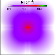
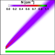
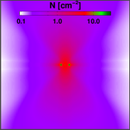
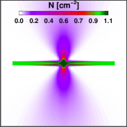
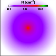
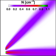
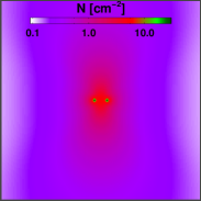
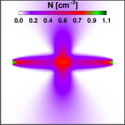
Fig. 1 illustrates the difference between the two flux functions in some idealized 2D RAMSES-RT tests, where we shoot off beams and turn on isotropic sources. Here the photon-gas interaction is turned off by setting all photoionization cross sections to zero (${\sigma}^{\rm{N}}_{j}={\sigma}^{\rm{E}}_{j}=0$ for any species $j$). It can be seen that the HLL flux function fails to give isotropic radiation (far left) and that the GLF function gives more diffusive beams (second from left). Note also how the diffusivity of beams with the HLL flux function is direction-dependent. A horizontal or vertical beam is perfectly retained while a diagonal one “leaks” to the sides almost as much as with the GLF function, which has the advantage of being fairly consistent on whether the beam is along-axis or diagonal. The right frames of the figure give an idea of how the radiative transport behaves in the case of multiple sources, i.e. with opposing beams and neighboring isotropic sources. The two opposing beams example is a typical configuration where the M1 closure relation obviously fails, creating a spurious source of radiation, perpendicular to the beam direction: Since opposing fluxes cannot cross each other in a single point in the moment approximation, the radiation is “squeezed” into those perpendicular directions. It is unclear to us how much of a problem this presents in astrophysical contexts. Beams, which clearly represent the worst case scenario, are not very relevant, but multiple nearby sources are. We generally prefer to use the GLF flux function, since we mostly deal with isotropic sources in our cosmological/galactic simulations, but the choice of function really depends on the problem. There is no noticeable difference in the computational load, so if shadows are important, one should go for HLL. AT08 have compared the two flux functions in some of the benchmark RT tests of Iliev et al. (2006a) and found that they give very similar results. We do likewise for the test we describe in §6.7, and come to the same conclusion.

3.3 The thermochemical step

Here we solve for the interaction between photons and gas. This is done by solving (6) and (7) with zero divergence and stellar injection terms.

Photon absorption and emission have the effect of heating and cooling the gas, so in order to self-consistently implement these interactions, we evolve along with them the thermal energy density ${\varepsilon}$ of the gas and the abundances of the species that interact with the photons, here Hi, Hei and Heii via photoionizations and Hii, Heii (again) and Heiii via recombinations. We follow these abundances in the form of the three ionization fractions $x_{\rm{H\scriptscriptstyle II}}$, $x_{\rm{He\scriptscriptstyle II}}$ and $x_{\rm{He\scriptscriptstyle III}}$, that we presented in Eqs. (15). The set of non-equilibrium thermochemistry equations solved in RAMSES-RT consists of:

$$\frac{\partial N_{i}}{\partial t} =-\sum_{j}^{{\rm{H\textsc{i}}},{\rm{He\textsc{i}}},\rm{He\textsc{ii}}}{n_{j}c{\sigma}^{\rm{N}}_{ij}N_{i}}$$ (25)

$$+\sum_{j}^{\rm{H\textsc{ii}},\rm{He\textsc{ii}},\rm{He\textsc{iii}}}b^{rec}_{ji}\,[\alpha^{\rm{A}}_{j}-\alpha^{\rm{B}}_{j}]\,n_{j}\,n_{e},$$

$$\frac{\partial{\bf{F}}_{i}}{\partial t} =-\sum_{j}^{{\rm{H\textsc{i}}},{\rm{He\textsc{i}}},\rm{He\textsc{ii}}}{n_{j}c{\sigma}^{\rm{N}}_{ij}{\bf{F}}_{i}},$$ (26)

$$\frac{\partial{\varepsilon}}{\partial t} ={\mathcal{H}}+{\mathcal{L}}$$ (27)

$$n_{\rm{H}}\frac{{\partial}x_{\rm{H\scriptscriptstyle II}}}{{\partial t}} =n_{\rm{H\scriptscriptstyle I}}\left(\beta_{{\rm{H\textsc{i}}}}\ n_{\rm{e}}+\sum_{i=1}^{M}{\sigma}^{\rm{N}}_{i{\rm{H\textsc{i}}}}cN_{i}\right)$$ (28)

$$-n_{\rm{H\scriptscriptstyle II}}\ \alpha^{\rm{A}}_{\rm{H\scriptscriptstyle II}}\ n_{\rm{e}},$$

$$n_{\rm{He}}\frac{{\partial}x_{\rm{He\scriptscriptstyle II}}}{{\partial t}} =n_{\rm{He\scriptscriptstyle I}}\left(\beta_{{\rm{He\textsc{i}}}}\ n_{\rm{e}}+\sum_{i=1}^{M}{\sigma}^{\rm{N}}_{i{\rm{He\textsc{i}}}}cN_{i}\right)$$ (29)

$$+n_{\rm{He\scriptscriptstyle III}}\ \alpha^{\rm{A}}_{\rm{He\textsc{iii}}}\ n_{\rm{e}}$$

$$-n_{\rm{He\scriptscriptstyle II}}\left(\beta_{\rm{He\textsc{ii}}}n_{\rm{e}}+\alpha^{\rm{A}}_{\rm{He\textsc{ii}}}n_{\rm{e}}+\sum_{i=1}^{M}{\sigma}^{\rm{N}}_{i\rm{He\textsc{ii}}}cN_{i}\right)$$

$$n_{\rm{He}}\frac{{\partial}x_{\rm{He\scriptscriptstyle III}}}{{\partial t}} =n_{\rm{He\scriptscriptstyle II}}\left(\beta_{\rm{He\textsc{ii}}}\ n_{\rm{e}}+\sum_{i=1}^{M}{\sigma}^{\rm{N}}_{i\rm{He\textsc{ii}}}cN_{i}\right)$$ (30)

$$-\ n_{\rm{He\scriptscriptstyle III}}\ \alpha^{\rm{A}}_{\rm{He\textsc{iii}}}\ n_{\rm{e}}$$

In the photon density and flux equations, (25) and (26), we have replaced the photon emission rate ${\dot{N}}^{rec}_{i}$ with the full expression for recombinative emissions from gas. Here, $\alpha^{\rm{A}}_{j}(T)$ and $\alpha^{\rm{B}}_{j}(T)$ represent case A and B recombination rates for electrons combining with species $j$ ($=\rm{H\textsc{ii}},\rm{He\textsc{ii}},\rm{He\textsc{iii}}$). The $b^{rec}_{ji}$ factor is a boolean (1/0) that states which photon group $j$-species recombinations emit into, and $n_{\rm{e}}$ is electron number density (a direct function of the H and He ionization states, neglecting the contribution from metals).

The temperature-evolution, (27) is greatly simplified here (see Appendix A for details). Basically it consists of two terms: the photoheating rate ${\mathcal{H}}(N_{i},x_{\rm{H\scriptscriptstyle II}},x_{\rm{He\scriptscriptstyle II}},x_{\rm{He\scriptscriptstyle III}},n_{\rm{H}})$ and the radiative cooling rate ${\mathcal{L}}(T,N_{i},x_{\rm{H\scriptscriptstyle II}},x_{\rm{He\scriptscriptstyle II}},x_{\rm{He\scriptscriptstyle III}},n_{\rm{H}})$.

The $x_{\rm{H\scriptscriptstyle II}}{}$ evolution (28) consists of, respectively on the RHS, Hi collisional ionizations, Hi photo-ionizations, and Hii recombinations. Here, $\beta(T)$ is a rate of collisional ionizations. The $x_{\rm{He\scriptscriptstyle II}}$ evolution (29) consists of, from left to right, Hei collisional ionizations, Heiii recombinations, Hei photo-ionizations, and Heii collisional ionizations, recombinations, and photoionizations. Likewise, the $x_{\rm{He\scriptscriptstyle III}}$ evolution (30) consists of Heii collisional ionizations and photoionizations, and Heiii recombinations. The expressions we use for rates of recombinations and collisional ionizations are given in Appendix E.

The computational approach we use to solving Equations (25)-(30) takes inspiration from Anninos et al. (1997). The basic premise is to solve the equations over a sub-step in a specific order (the order we have given), explicitly for those variables that remain to be solved (including the current one), but implicitly for those that have already be solved over the sub-step. Eqs. (25) and (26) are thus solved purely explicitly, using the backwards-in-time (BW) values for all variables on the RHS. Eq. (27) is partly implicit in the sense that it uses forward-in-time values for $N$ and ${\bf{F}}$, but BW values for the other variables. And so on, ending with Eq. (30), which is then implicit in every variable except the one solved for ($x_{\rm{He\scriptscriptstyle III}}$). We give details of the discretization of these equations in Appendix A.

3.3.1 The 10% thermochemistry rule

For accuracy, each thermochemistry step is restricted by a local cooling time which prohibits any of the thermochemical quantities to change by a substantial fraction in one time-step. We therefore sub-cycle the thermochemistry step to fill in the global RT time-step (see next section), using what can be called the $10\%$ rule: In each cell, the thermochemistry step is initially executed with the full RT time-step length, and then the fractional update is considered. If any of the evolved quantities ($N_{i},F_{i}$, ${\varepsilon}$, ionization fractions) have changed by more than $10\%$, we backtrack and do the same calculation with half the time-step length. Conversely, if the greatest fractional change in a sub-step is $<5\%$, the timestep length is doubled for the next sub-step (without the backtracking).

Together, the quasi-implicit approach used in solving the thermochemistry, and the $10\%$ rule, infer that photons are in principle conserved only at the $10\%$ level. This is because the thermochemistry solver is explicit in the photon density updates (i.e. uses before-timestep values of ionization fractions), but the following ionization fraction updates are implicit in the photon densities (i.e. they use after-timestep values for the photon densities). Thus, in the situation of a cell in the process of being photoionized, the ionization fractions are underestimated at the photon density updates and the photon densities are underestimated at the ionization fraction updates. Conversely, if the cell gas is recombining, the recombination-photon emission is slightly overestimated, since before-timestep values for the ionization fractions are used for the emissivity. However, judging from the performance in RT tests (§6) and thermochemistry tests (§C), this does not appear to be cause for concern.

3.3.2 The on-the-spot approximation

The photon-emitting recombinative term, the second RHS sum in (25), is optionally included. Excluding it is usually referred to as the on-the-spot approximation (OTSA), meaning that any recombination-emitted photons are absorbed “on the spot” by a near-lying atom (in the same cell), and hence these photon emissions cancel out by local photon absorptions. If the OTSA is assumed, the gas is thus not photoemitting, and the case A recombination rates are replaced with case B recombination rates in (25)-(30), i.e. photon-emitting recombinations straight down to the ground level are not counted. The OTSA is in general a valid approximation in the optically thick regime but not so when the photon mean free path becomes longer than the cell width.

It is a great advantage of our RT implementation that it is not restricted to a limited number of point sources. The computational load does not scale at all with the number of sources, and photon emission from gas (non-OTSA) comes at no added cost, whereas it may become prohibitively expensive in ray-tracing implementations.

4 Timestepping issues

RT is computationally expensive, and we use two basic tricks to speed up the calculation. One is to reduce the speed of light, the other is to modify slightly the traditional operator splitting approach, by increasing the coupling between photon injection and advection on one hand and thermochemistry and photo-heating on the other hand.

4.1 The RT timestep and the reduced speed of light

In each iteration before the three RT steps of photon injection, advection and thermochemistry are executed, the length of the time-step, $\Delta t_{\rm{RT}}$, must be determined.

We use an explicit solver for the radiative transport (21), so the advection timestep, and thus the global RT timestep, is constrained by the Courant condition (here in 3D),

$$\Delta t_{\rm{RT}}<\frac{\Delta x}{3c},$$ (31)

where $\Delta x$ is the cell width. This time-step constraint is severe: it results in an integration step which is typically 300 times shorter than in non-relativistic hydrodynamical simulations, where the speed of light is replaced by a maximum gas velocity ($\sim 1000\ km/s$) in Eq. 45. In a coupled (RHD) simulation, this would imply a comparable increase in CPU time, either because of a global timestep reduction (as we chose to implement, see Sec. 5), or because of many radiative sub-steps (as is implemented e.g. in ATON). In the case of radiative transfer with the moment equations, there are two well-known solutions to this problem.

The first solution is to use an implicit method instead of an explicit one to solve the transport equation, which means using forward-in-time intercell fluxes in (21), i.e replacing ${\mathcal{F}}^{n}\equiv{\mathcal{F}}^{t}$ with ${\mathcal{F}}^{n+1}\equiv{\mathcal{F}}^{t+\Delta t}$. This seemingly simple change ensures that the computation is always stable, no matter how big the time-step, and we can get rid of the Courant condition. However: (i) It doesn’t mean that the computation is accurate, and in fact we still need some time-stepping condition to retain the accuracy, e.g. to restrain any quantity to be changed by more than say $10\%$ in a single time-step. Furthermore, such a condition usually must be checked by trial-and-error, i.e. one guesses a time-step and performs a global transport step (over the grid) and then checks whether the accuracy constraint was broken anywhere. Such trial-and-error time-stepping can be very expensive since it is a global process. (ii) Replacing ${\mathcal{F}}^{t}$ with ${\mathcal{F}}^{t+\Delta t}$ is actually not simple at all. Eqs. 21 become a system of coupled algebraic equations that must be solved via matrix manipulation in an iterative process, which is complicated, computationally expensive, and of limited scope (i.e. can’t be easily applied to any problem). Due to these two reasons we have opted out of the implicit approach. It is absolutely a valid approach however, and used by many (e.g. Petkova & Springel, 2009; Commerçon et al., 2011).

The second solution, which we have chosen instead, is to keep our solver explicit, and relax the Courant condition by changing the speed of light to a reduced light speed ${c_{r}}\ll c$, the payoff being that the time-step (45) becomes longer. This is generally referred to as the reduced speed of light approximation (RSLA), and was introduced by Gnedin & Abel (2001). The idea of the RSLA is that in many applications of interest, the propagation of light is in fact limited by the much slower speed of ionizing fronts. In such situations, reducing the speed of light, while keeping it higher than the fastest I-front, will yield the correct solution at a much reduced CPU cost. In the following section, we provide a framework to help judge how accurate the RSLA may be in various astrophysical contexts.

4.2 A framework for setting the reduced light speed value

In the extremely complex framework of galaxy formation simulations, the accuracy of the results obtained using the RSLA can really only be assessed by convergence tests. It is nonetheless useful to consider a simple idealized setup in order to derive a physical intuition of where, when, and by how much one may reduce the speed of light. In this section, we thus discuss the expansion of an ionized region around a central source embedded in a uniform neutral medium.

We consider a source turning on and emitting ionizing photons at a rate ${\dot{N}}$ into a homogeneous hydrogen-only medium of number density $n_{\rm{H}}$. An expanding sphere of ionized gas forms around the source and halts at the Strömgren radius $r_{\rm{S}}$ within which the rate of recombinations equals the source luminosity:

$$r_{\rm{S}}=\left(\frac{3{\dot{N}}}{4\pi\alpha^{\rm{B}}n_{\rm{H}}^{2}}\right)^{1/3},$$ (32)

where $\alpha^{\rm{B}}\sim 2.6\times 10^{-13}\ \rm{cm}^{3}\,\rm{s}^{-1}$ is the case-B recombination rate at $T\sim 10^{4}\ K$, and where we have assumed that the plasma within $r_{\rm{S}}$ is fully ionized.

The relativistic expansion of the I-front to its final radius $r_{\rm{S}}$ is derived in Shapiro et al. (2006), and may be expressed as:

$$w=qy-\ln(1-y^{3}),$$ (33)

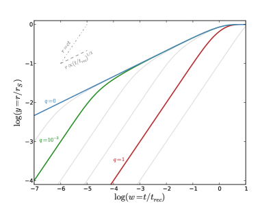
where $w=t/t_{\rm{rec}}$ is time in units of the recombination time $t_{\rm{rec}}=(n_{\rm{H}}\alpha^{\rm{B}})^{-1}$, $y=r_{\rm{I}}/r_{\rm{S}}$ is the position of the I-front in units of $r_{\rm{S}}$, and the factor $q\equiv t_{\rm{cross}}/t_{\rm{rec}}\equiv r_{\rm{S}}/(ct_{\rm{rec}})$ describes the light crossing time $t_{\rm{cross}}$ across the Strömgren radius in units of the recombination time, and basically encompasses all the free parameters in the setup (source luminosity, gas density, and temperature). Writing $q\propto{\dot{N}}^{1/3}n_{\rm{H}}^{1/3}$, we see that in many astrophysical contexts, $q$ stays in the range $\sim 10^{-3}-10^{-2}$ (see Table 1), simply because we are generally either interested in the effect of bright sources (e.g. a whole galaxy) on relatively low-density gas (e.g. the IGM) or of fainter sources (e.g. an O-star) on high-density gas (at e.g. molecular-cloud densities).

Let us now discuss briefly the evolution of an I-front given by Eq. 33 for illustrative values of $q$:

• $q=0$ (blue curve of Fig. 2): this is the limiting non-relativistic case, which assumes an infinite speed of light ($t_{\rm{cross}}=0$). In this case, the I-front expands roughly as $y\propto w^{1/3}$ (its speed decreases as $w^{-2/3}$) almost all the way to $r_{\rm{S}}$, which it reaches after about a recombination time.

• $q=1$ (red curve of Fig. 2): here (and for all $q>1$), the I-front basically expands at the speed of light all the way to $r_{\rm{S}}$, which it thus reaches after a crossing time (which is equal to a recombination time in this case).

• $q=10^{-3}$ (green curve of Fig. 2): in this typical case, the I-front starts expanding at the speed of light, until $w\sim(q/3)^{3/2}$. It then slows down and quickly reaches the limiting $q=0$ behavior after a crossing time (at $w\sim q$). The I-front then reaches $r_{\rm{S}}$ after a recombination time (at $w\sim 1$).

An important feature appearing in the two latter cases is that for any physical setup $q>0$, the I-front is always well described by the $q=0$ limit after a crossing time (i.e. $w\gtrsim q$). We can use this feature to understand the impact of reducing the speed of light in our code. Say we have a physical setup described by a value $q_{0}$. Reducing the speed of light by a factor ${f_{c}}<1$ ($c_{r}={f_{c}}c$) implies an increase by a factor $1/{f_{c}}$ of the effective crossing time, and the effective $q$ in our experiment becomes $q_{0}/{f_{c}}$. The solution we obtain with $c_{r}$ will be accurate only after an effective crossing time, i.e. after $w=q_{0}/{f_{c}}$. Before that time, the reduced-light-speed solution will lag behind the real one.

How much one may reduce the speed of light in a given numerical experiment then depends on the boundary conditions of the problem and their associated timescales. Call $\tau_{\rm sim}$ the shortest relevant timescale of a simulation. For example, if one is interested in the effect of radiative feedback from massive stars onto the ISM, $\tau_{\rm sim}$ can be set to the lifetime of these stars. If one is running a very short experiment (see Sec. 6.5), the duration of the simulation may determine $\tau_{\rm sim}$. Given this timescale contraint $\tau_{\rm sim}$, one may reduce the speed of light by a factor such that the I-fronts will be correctly described after a timelapse well shorter than $\tau_{\rm sim}$, i.e. $t_{\rm{cross}}/{f_{c}}\ll\tau_{\rm sim}$. In other words, one may typically use ${f_{c}}=\min(1;\sim 10\times t_{\rm{cross}}/\tau_{\rm sim})$. We now turn to a couple of concrete examples.

Figure 2: I-front expansion in a Stromgren sphere for a set of values of the dimensionless crossing time $q$. The blue curve shows the infinite-light-speed limit ($q=0$). The green curve shows a typical case with $q=10^{-3}$, and the red curve shows the $q=1$ case, as discussed in the text. The thin grey curves show other values of $q$, spanning the range $10^{-4}-10$ in steps of one dex. The grey lines in the top-left corner of the plot show slopes corresponding to an expansion at the speed of light (dot-dashed line) or as $(t/t_{\rm{rec}})^{1/3}$ (dashed line). For any $q>0$, the I-front radius is accurately described by the $q=0$-limit after a crossing time.

Table 1: Strömgren sphere properties for typical cosmological regimes, with the inferred minimum allowed light speed fractions.

Regime	$n_{\rm{H}}$ [${\rm{cm}}^{-3}$]	${\dot{N}}$ [$\rm{s}^{-1}$]	$r_{\rm{S}}$ [kpc]	$t_{\rm{cross}}$ [Myr]	$t_{\rm{rec}}$ [Myr]	$q$	$\tau_{\rm sim}$ [Myr]	$w_{\rm{sim}}$	$f_{\rm{c,min}}$
MW ISM	$10^{-1}$	$2\ 10^{50}$	$0.9$	$3\ 10^{-3}$	$1.2$	$2\ 10^{-3}$	$1$	$1$	$3\ 10^{-2}$
MW cloud	$10^{2}$	$2\ 10^{48}$	$2\ 10^{-3}$	$6\ 10^{-6}$	$1\ 10^{-3}$	$5\ 10^{-3}$	$0.1$	$80$	$6\ 10^{-4}$
Iliev tests 1,2,5	$10^{-3}$	$5\ 10^{48}$	$5.4$	$2\ 10^{-2}$	$122.3$	$1.4\ 10^{-4}$	$10$	$8\ 10^{-2}$	$2\ 10^{-2}$
Iliev test 4	$10^{-4}$	$7\ 10^{52}$	$600$	$2$	$1200$	$2\ 10^{-3}$	$0.05$	$4\ 10^{-5}$	$1$

4.3 Example speed of light calculations

In Table 1 we take some concrete (and of course very approximate) examples to see generally what values of ${f_{c}}$ are feasible. We consider cosmological applications from inter-galactic to inter-stellar scales and setups from some of the RT code tests described in §6.

Reionization of the inter-galactic medium

Here we are concerned with the expansion of ionization fronts away from galaxies and into the IGM, as for example in the fourth test of Iliev et al. (2006a) (hereafter Il06). In this test, the IGM gas density is typically $n_{\rm{H}}=10^{-4}$ cm^-3, and the sources have $\dot{N}=7\ 10^{52}\ s^{-1}$. In such a configuration, the Strömgren radius is $r_{\rm{S}}\sim 600$ kpc, corresponding to a crossing time $t_{\rm{cross}}\sim 2$ Myr. Because of the low density of the gas, the recombination time is very long ($\gtrsim 1$ Gyr), and we are thus close to the $q=10^{-3}$ case discussed above (the green curve in Fig. 2).

Test 4 of Il06 is analyzed at output times $\tau_{\rm sim,1}=0.05$ Myr and $\tau_{\rm sim,2}=0.4$ Myr (see Fig. 19). In both cases, $\tau_{\rm sim}<t_{\rm{cross}}$, and we cannot reduce the speed of light to get an accurate result at these times, because the expanding front has not yet reached the $q=0$ limit. Interestingly, we cannot increase the speed of light either, as is done in Il06 with C²-Ray which assumes an infinite light-speed. From Fig. 2, it is clear that this approximation (the blue curve) will over-predict the radius of the front. We can use the analysis above to note that had the results been compared at a later output time $\tau_{\rm sim}>2$ Myr, the infinite-light-speed approximation would have provided accurate results. It is only ten times later, however, that reducing the speed of light by a factor ten would have provided accurate results.

We conclude that propagating an I-front in the IGM at the proper speed requires to use a value of the speed of light close to the correct value. This is especially true in Test 4 of the Il06 paper (last row of Table 1). This confirms that for cosmic reionization related studies, using the correct value for the speed of light is very important.

Inter-stellar medium

There is admittedly a lot of variety here, but as a rough estimate, we can take typical densities to be $n_{\rm{H}}\sim 10^{-1}\ {\rm{cm}}^{-3}$ in the large-scale ISM and $n_{\rm{H}}\sim 10^{2}\ {\rm{cm}}^{-3}$ in star-forming clouds. In the stellar nurseries we consider single OB stars, releasing ${\dot{N}}_{OB}\sim 2\times 10^{48}$ photons per second, and in the large-scale ISM we consider groups of ($\sim 100$) OB stars. The constraining timescale is on the order of the stellar cycle of OB stars ($\tau_{\rm sim}\sim~{}10$ Myr), and less for the stellar nurseries. In these two cases, which are representative of the dense ISM inside galactic disks, we see in Table 1 that the allowed reduction factor for the speed of light is much larger ($f_{c}\simeq 10^{-4}$ to $10^{-3}$). This is due to two effects acting together: the gas density is higher, but the sources are fainter, since we are now resolving individual stellar clusters, and not an entire galaxy. Tests 1, 2 of Il06 and test 5 of its’ RHD sequel (Iliev et al., 2009) are also representative of such a favorable regime to use the reduced speed of light approximation (second to last row in Table 1). This rigorous analysis of the problem at hand confirms that propagating I-front in galaxy formation simulation can be done reliably using our current approach, while cosmic reionization problems are better handled with GPU acceleration and the correct speed of light.

4.4 Smoothed RT

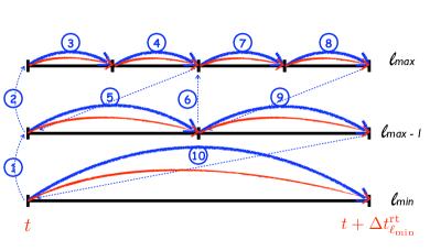
A problem we had to face, while performing RAMSES-RT galaxy formation runs, as well as the various test cases presented here, is that there is often a small number of cells, usually along I-fronts, or close to strong radiation sources, that execute a huge number of thermochemistry subcycles in a single RT time-step. This is in part fault of the operator-splitting approach used, where the RT equations have been partly decoupled. Specifically, the photon density updates happen in three steps in this approach (see Fig. 3, top). The photon injection step always increases the number of photons, usually by a relatively large amount, and the transport step does the same when it feeds photons into cells along these I-fronts. The thermochemistry step in the I-front cells has the exact opposite effect: the photon density decreases again via absorptions. If the photon-depletion time is shorter than the Courant time, we have a curious situation where the cell goes through an inefficient cycle during the thermochemistry subcycles: it starts neutral with a large abundance of photons (that have come in via the transport and/or photon injection steps). It first requires a number of subcycles to evolve to a (partly) ionized state, during which the photon density is gradually decreased. It can then reach a turnaround when the photons are depleted. If the RT time-step is not yet finished, the cell then goes into a reverse process, where it becomes neutral again. This whole cycle may take a large number of thermochemical steps, yet the cell gas ends up being in much the same state as it started.

In reality, the ionization state and photon density would not cycle like this but would rather settle into a semi-equilibrium where the rate of ionizations equals that of recombinations.

(a)

(b)

Figure 3: Sketch plots showing a photon density evolution over a global RT time-step with normal RT (top) and smoothed RT (bottom). In normal RT the photon density is updated to $N^{\prime}$ during photon transport (a) and injection (b). This is then used as an initial state for thermochemistry (c). It is often the case that the photons are depleted over the global time-step $\Delta t$, in a process which takes many thermochemistry subcycles. In smoothed RT, the photon density state is not updated by the transport and injection steps, but rather the difference is used to infer a photon injection rate for the cell, which is gradually added during each thermochemistry substep. This can dramatically reduce the needed number of chemistry substeps.

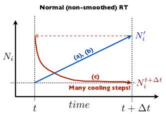
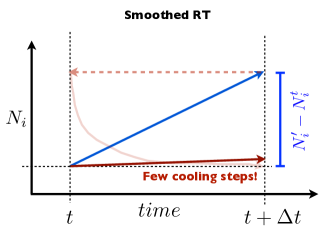
For the purpose of saving up on computing time and reducing the number of thermochemistry subcycles, we have implemented an optional strategy we call smoothed RT that roughly corrects this non-equilibrium effect of operator splitting (see Fig. 3, bottom). In it, the result of ($N^{\prime}_{i},{\bf{F}}^{\prime}_{i}$) from the transport and injection steps in each cell is used to infer a rate for the thermochemistry step, rather than being set as an initial condition. We use the pre-transport, pre-injection values of $N^{t}_{i}$ and ${\bf{F}}^{t}_{i}$ as initial conditions for the thermochemistry, but instead update the thermochemistry equations (25) and (26) to

$$\frac{\partial N_{i}}{\partial t} =-\sum_{j}^{{\rm{H\textsc{i}}},{\rm{He\textsc{i}}},\rm{He\textsc{ii}}}{n_{j}c{\sigma}^{\rm{N}}_{ij}N_{i}}\ \ +\ {\dot{N}}^{rec}_{i}\ +\ \dot{N}_{i},$$ (34)

$$\frac{\partial{\bf{F}}_{i}}{\partial t} =-\sum_{j}^{{\rm{H\textsc{i}}},{\rm{He\textsc{i}}},\rm{He\textsc{ii}}}{n_{j}c{\sigma}^{\rm{N}}_{ij}{\bf{F}}_{i}}\ +\ \dot{{\bf{F}}}_{i},$$ (35)

where the new terms at the far right represent the rates at which the photon densities and fluxes changed in the transport and injection steps, i.e.

$$\dot{N}_{i}=\frac{N_{i}^{\prime}-N^{t}_{i}}{\Delta t},$$ (36)

$$\dot{{\bf{F}}}_{i}=\frac{{\bf{F}}_{i}^{\prime}-{\bf{F}}^{t}_{i}}{\Delta t},$$ (37)

where $N^{t}_{i}$ and ${\bf{F}}^{t}_{i}$ ($N_{i}^{\prime}$ and ${\bf{F}}_{i}^{\prime}$) denote a cell state before (after) cell injection (Eq. 16) and transport (Eqs. 18 and 19) have been solved over $\Delta t$. The injection and transport steps are unchanged from the normal operator splitting method, except for the fact that the cell states are not immediately updated to reflect the end results of those steps. The results of the injection step go only as initial conditions into the transport step, and the end results of the transport step are only used to calculate the photon density and flux rates of change via Eqs. (36) and (37). Only after the thermochemistry step does a cell get a valid state that is the result of all three steps.

The idea is that when the photons are introduced like this into the thermochemistry step, they will be introduced gradually in line with the subcycling, and the photon density vs. ionization fraction cycle will disappear as a result and be replaced with a semi-equilibrium, which should reduce the number of subcycles and the computational load. The total photon injection (or depletion) will still equal $N_{i}^{\prime}-N^{t}_{i}$, so in the limit that there are no photoionizations or photon-emitting recombinations, the end result is exactly the same photon density (and flux) as would be left at the end of the transport and injection steps without smoothed RT.

The advantage of the smoothing approach is perhaps best explained with an example: consider a cell with a strong source of radiation and gas dense and neutral enough that the timescales of cooling, ionization and/or recombination are much shorter than the global timestep length, $\Delta t$. This could either be a source containing a stellar particle or a cell along an ionization front. Without smoothing, the photoionization rate in the cell can change dramatically as a result of photon injection/transport. The thermochemistry step thus starts with a high rate of photoionzations which gradually goes down in the thermochemistry sub-cycling as the gas becomes more ionized and the photons are absorbed. With smoothing, this dramatic change in the photoionization rate never happens, thus requiring fewer thermochemistry sub-cycles to react. A situation also exists where the smoothing approach slows down the thermochemistry: if a cell contains a strong source of radiation, but diffuse gas (i.e. long timescales compared to $\Delta t$ for cooling, ionization and/or recombination), the non-smoothed approach would result in little or no thermochemistry sub-cycling, whereas the smoothed approach would take many sub-cycles just to update the radiation field and effectively reach the final result of the injection and transport steps.

The gain in computational speed is thus quite dependent on the problem at hand, and also on the reduced light speed, which determines the size of the RT time-step, $\Delta t$. We’ve made a comparison on the computational speed between using the smoothed and non-smoothed RT in a cosmological zoom simulation from the NUT simulations suite (e.g. Powell, Slyz & Devriendt, 2011) that includes the transfer of UV photons from stellar sources. Here, smoothed RT reduces the average number of thermochemistry subcycles by a factor of $6$ and the computing time by a factor $3.5$. So a lot may indeed be gained by using smoothed RT.

One could argue that the ionization states in I-fronts are better modelled with smoothed RT, since the cycle of photon density and ionization fraction is a purely numerical effect of operator splitting. We have intentionally drawn a slightly higher end value of $N_{i}$ in the smoothed RT than non-smoothed in Fig. 3: whereas non-smoothed RT can completely deplete the photons in a cell, smoothed RT usually leaves a small reservoir after the thermochemistry, that more accurately represents the “semi-equilibrium value”.

Of course an alternative to smoothed RT, and a more correct solution, is to attack the root of the problem and reduce the global time-step length, i.e. also limit the transport and injection steps to the $10\%$ rule. Reducing the global time-step length is highly impractical though; the main reason for using operator splitting in the first place is that it enables us to separate the timescales for the different steps.

The same method of smoothing out discreteness that comes with operator splitting (in the case of pure hydrodynamics) has previously been described by Sun (1996), where it is referred to as “pseudo-non-time-splitting”.

5 Radiation hydrodynamics in Ramses

RAMSES (Teyssier, 2002) is a cosmological adaptive mesh refinement (AMR) code that can simulate the evolution and interaction of dark matter, stellar populations and baryonic gas via gravity, hydrodynamics and radiative cooling. It can run on parallel computers using the message passing interface (MPI) standard, and is optimized to run very large numerical experiments. It is used for cosmological simulations in the framework of the expanding Universe, and also smaller scale simulations of more isolated phenomena, such as the formation and evolution of galaxies, clusters, and stars. Dark matter and stars are modelled as collisionless particles that move around the simulation box and interact via gravity. We will focus here on the hydrodynamics of RAMSES though, which is where the RT couples to everything else.

RAMSES employs a second-order Godunov solver on the Euler equations of gravito hydrodynamics in their conservative form,

$$\frac{\partial\rho}{\partial t}+\nabla\cdot\left(\rho{\bf{u}}\right) =0$$ (38)

$$\frac{\partial}{\partial t}\left(\rho{\bf{u}}\right)+\nabla\cdot\left(\rho{\bf{u}}\otimes{\bf{u}}\right)+\nabla P =-\rho\nabla\phi$$ (39)

$$\frac{\partial E}{\partial t}+\nabla\cdot\left(\left(E+P\right){\bf{u}}\right) =-\rho{\bf{u}}\cdot\nabla\phi+\Lambda(\rho,{\varepsilon}),$$ (40)

where $t$ is time, $\rho$ the gas density, ${\bf{u}}$ the bulk velocity, $\phi$ the gravitational potential, $E$ the gas total energy density, $P$ the pressure, and $\Lambda$ represents radiative cooling and heating via thermochemistry terms (resp. negative and positive), which are functions of the gas density, temperature and ionization state. In RAMSES, collisional ionization equilibrium (CIE) is traditionally assumed, which allows the ionization states to be calculated as surjective functions of the temperature and density and thus they don’t need to be explicitly tracked in the code. $E$ is divided into kinetic and thermal energy density (${\varepsilon}$) components:

$$E=\frac{1}{2}\rho u^{2}+{\varepsilon}.$$ (41)

The system of Euler equations is closed with an equation of state which relates the pressure and thermal energy,

$$P=(\gamma-1){\varepsilon},$$ (42)

where $\gamma$ is the ratio of specific heats. The Euler equations are adapted to super comoving coordinates, to account for cosmological expansion, by a simple transformation of variables (see §5.4).

The Euler equations are solved across an AMR grid structure. Operator splitting is employed for the thermochemistry source terms, i.e. $\Lambda$ is separated from the rest of the Euler equations in the numerical implementation – which makes it trivial to modify the thermochemistry solver, i.e. change it from equilibrium to non-equilibrium.

Figure 4: An oct – the basic grid element in RAMSES.

The basic grid element in RAMSES is an oct (Fig. 4), which is a grid composed of eight cubical cells. A conservative state vector ${\mathcal{U}}=(\rho,\rho{\bf{u}},E,\rho Z)$ is associated with each cell storing its hydrodynamical properties of gas density $\rho$, momentum density $\rho{\bf{u}}$, total energy density $E$ and metal mass density $\rho Z$. (One can also use the primitive state vector, defined as ${\cal W}=(\rho,{\bf{u}},P,Z)$.) Each cell in the oct can be recursively refined to contain sub-octs, up to a maximum level $\ell$ of refinement. The whole RAMSES simulation box is one oct at $\ell=1$, which is homogeneously and recursively refined to a minimum refinement level $\ell_{\rm{min}}$, such that the coarse (minimum) box resolution is $2^{\ell_{\rm{min}}}$ cells on each side. Octs at or above level $\ell_{\rm{min}}$ are then adaptively refined during the simulation run, to follow the formation and evolution of structures, up to a maximum refinement level $\ell_{\rm{max}}$, giving the box a maximum effective resolution of $2^{\ell_{\rm{max}}}$ cell widths per box width. The cell refinement is gradual: the resolution must never change by more than one level across cell boundaries.

5.1 RAMSES multi-stepping approach

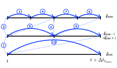
With AMR multi-stepping, the resolution is not only adaptive in terms of volume, but also in time, with different timestep sizes on different refinement levels. A coarse time-step, over the whole AMR grid, is initiated at the coarse level, $\ell_{\rm{min}}$, as we show schematically in Fig. 5. First, the coarse time-step length $\Delta t_{\ell_{\rm{min}}}$ is estimated via (the minimum of) Courant conditions in all $\ell_{\rm{min}}$ cells. Before the coarse step is executed, the next finer level, $\ell_{\rm{min}}+1$, is made to execute the same time-step, in two substeps since the finer level Courant condition should approximately halve the time-step length. This process is recursive: the next finer level makes its own time-step estimate (Courant condition, but also $\Delta t_{\ell}\leq\Delta t_{\ell-1}$) and has its next finer level to execute two substeps. This recursive call up the level hierarchy continues to the highest available level $\ell_{\rm{max}}$, which contains only leaf cells and no sub-octs. Here the first two substeps are finally executed, with step lengths $\Delta t_{\ell_{\rm{max}}}\leq\Delta t_{\ell_{\rm{min}}}/2^{\ell_{\rm{max}}-\ell_{\rm{min}}}$. When the two $\ell_{\rm{max}}$ substeps are done, the $\ell_{\rm{max}}-1$ time-step is re-evaluated to be no longer than the sum of the two substeps just executed at $\ell_{\rm{max}}$, and then one $\ell_{\rm{max}}-1$ step is executed. Then back to level $\ell_{\rm{max}}$ to execute two steps, and so on. The substepping continues in this fashion across the level hierarchy, ending with one time-step for the coarsest level cells (with a modified time-step length $\Delta t_{\ell_{\rm{min}}}$).

At the heart of RAMSES lies a recursive routine called $\tt{amr\_step(\ell)}$ which describes a single time-step at level $\ell$, and is initially called from the coarsest level ($\ell_{\rm{min}}$). To facilitate our descriptions on how the RT implementation is placed into RAMSES, we illustrate the routine in pseudocode format in Listing 1, where we have excluded details and bits not directly relevant to RHD (e.g. MPI syncing and load-balancing, adaptive refinement and de-refinement, particle propagation, gravity solver, star formation, and stellar feedback).

First, the recursion is made twice, solving the hydrodynamics over two sub-steps at all finer levels. Then the Euler equations are solved over the current coarse time-step, for all cells belonging to the current level. It is important to note here that the hydrodynamical quantities are fully updated at the current level in the $\tt{hydro\_solver}$, but there are also intermediate hydro updates in all neighboring cells at the next coarser level. The coarser level update is only partial though, because it only reflects the intercell fluxes across inter-level boundaries, and fluxes across other boundaries (same level or next coarser level) will only be accounted for when the coarser level time-step is fully advanced. Until then, these coarser level neighbor cells have gas states that are not well defined, since they only reflect some of their intercell fluxes. It effectively means that at any point between the start and finish of the primary (coarse) call to $\tt{amr\_step}$, there are some cells in the simulation box (lying next to finer level cells) that have ill-defined intermediate hydrodynamical states. This point is further illustrated in Appendix D. It is important to keep in mind when considering the coupling of RT with the hydrodynamics of RAMSES.

Having put down the basics of AMR hydrodynamics, we are now in a position to add radiative transfer.

Figure 5: Recursive hydro time-stepping over one coarse time-step in the AMR levels of RAMSES, here shown for a three-level AMR structure. Each solid arrowed line represents a time-step which is executed for all cells belonging to the corresponding AMR level. The numbers indicate the order of the time-stepping, including the calls to finer levels (1, 2, and 6).

Listing 1: The AMR step in RAMSES.

⬇

recursive subroutine amr_step($\ell$):

if $\ell$ < $\ell_{\rm{max}}$ and any cells exist in $\ell+1$

call amr_step($\ell+1$)

call amr_step($\ell+1$)

call hydro_solver($\ell$): all $\ell$ cells and some $\ell-1$

call eq_thermochemistry($\ell$): all $\ell$ leaf cells

end

5.2 RAMSES-RT

In RAMSES-RT, each cell stores some additional state variables. Here ${{\mathcal{U}}}=(\rho,\rho{\bf{u}},E,\rho Z,\rho x_{\rm{H\scriptscriptstyle II}},\rho x_{\rm{He\scriptscriptstyle II}},\rho x_{\rm{He\scriptscriptstyle III}},N_{i},{\bf{F}}_{i})$, where $x_{\rm{H\scriptscriptstyle II}}{}$, $x_{\rm{He\scriptscriptstyle II}}{}$ and $x_{\rm{He\scriptscriptstyle III}}{}$ are the hydrogen and helium ionization fractions, which are advected with the gas as passive scalars (in the hydro solver), and $N_{i}$, ${\bf{F}}_{i}$ represent the $4M$ variables of photon density and flux for each of the $M$ photon groups. Note that this represents a hefty increase in the memory requirement compared to the hydrodynamics only of RAMSES: the memory requirement for storing ${\mathcal{U}}$ (which is the bulk of the total memory in most simulations) is increased by a factor of $1.5(1+4/9M)$, where the $1.5$ represents the ionization fractions and the parenthesis term represents the photon fluxes and densities. Thus, with three photon groups, the memory requirement is increased by roughly a factor $3.5$ compared to a traditional RAMSES simulation.

Given the time-scale difference between hydrodynamics and radiative transfer, the obvious approach to performing RHD is to sub-cycle the three radiative transfer steps (injection, advection, thermochemistry) within the hydrodynamical step. There is, however, a major drawback to this approach, which is that it is incompatible with AMR multi-stepping: the RT sub-cycling must be done before/after each hydrodynamical AMR step at the finest refinement level only, and since light can in principle cross the whole box within the fine level hydrodynamical timestep, the RT sub-cycling must be done over the whole grid, over all levels. However, the partial hydrodynamical flux between cells at level boundaries always leaves some cells between the fine level steps with an intermediate (i.e. partially updated) gas state. This makes the thermochemistry ill-defined in those cells, since it needs to update the gas temperature in every cell, and for this to work the temperature must have a well defined and unique value everywhere. There are three ways around this:

First is to perform the RT subcycling only after a coarse hydrodynamical step, but here potentially thousands of fine-scale hydro steps would be executed without taking into account the thermochemistry.

Figure 6: Diagram of the $\tt{amr\_step}$ in RAMSES-RT. This is much like the normal $\tt{amr\_step}$ in RAMSES, except that the time-step length has the extra constraint of the light speed Courant condition, and each level $\ell$ step also performs photon injection, RT transport and thermochemistry over the same time-step and level.

Listing 2: The AMR step in RAMSES-RT.

⬇

recursive subroutine amr_step($\ell$)

if $\ell$ < $\ell_{\rm{max}}$ and any cells in $\ell+1$

call amr_step($\ell+1$)

call amr_step($\ell+1$)

call photon_injection_step($\ell$)

call hydro_solver($\ell$): all $\ell$ cells and some $\ell-1$

call rt_transport($\ell$): all $\ell$ cells and some $\ell-1$

call neq_thermochemistry($\ell$): all $\ell$ leaf cells

end

Second, is to prohibit AMR multi-stepping, which makes the whole grid well defined after each step and thus allows for RT sub-cycling over the whole box. Multi-stepping is however one of the main advantages of AMR, and essentially allows us to refine in time as well as space, so this isn’t really an option.

We thus default to the third strategy, which we use in RAMSES-RT. Here we drop the subcycling of RT within the hydro step and perform the two on the same timestep length, which is the minimum of the RT and hydro timestep. Thus, with each hydro step, at any level, the RT steps are performed over the same level only. The basic scheme is illustrated in Fig. 6, and the pseudocode for the updated $\tt{amr\_step}$ is shown in Listing 2. Obviously, the main drawback here is the timescale difference, which can be something like a factor of $100-1000$, meaning the number of hydrodynamical steps is increased the same factor and the run-time accordingly (plus numerical diffusion likely becomes a problem with such small hydrodynamical time-steps). However, if we also apply a reduced speed of light, we can shrink this factor arbitrarily, down to the limit where the hydro-timestep is the limiting factor and the only increase in computational load is the added advection of photons (which is considerably cheaper for one photon group than the hydrodynamical solver) and the non-equilibrium thermochemistry (which typically has a computational cost comparable to the equilibrium solver of RAMSES, provided we use RT smoothing). The question, which we have tried to answer in §4.2, is then how far we are allowed to go in reducing the light speed.

Parallelization is naturally acquired in RAMSES-RT by simply taking advantage of the MPI strategies already in place in RAMSES.

5.3 Radiation transport on an AMR grid

In RAMSES-RT, the radiation variables are fully incorporated into the AMR structure of RAMSES. The ionization fractions and photon densities and fluxes are refined and de-refined along with the usual hydro quantities, with a choice of interpolation schemes for newly refined cells (straight injection or linear interpolation). The radiative transfer, i.e. injection, transport and thermochemistry, is multi-stepped across the level hierarchy, thus giving AMR refinement both in space and time. Inter-level radiation transport is tackled in the same way as the hydrodynamical advection, i.e. transport on level $\ell$ includes partial updates of neighbouring cells on level $\ell-1$. Update of the finer level cell RT variables over level boundaries involves the RT variables in a coarser cell, which are evaluated, again with the same choice of interpolation schemes. RAMSES-RT includes optional refinement criteria on photon densities, ion abundances and gradients in those, in addition to the usual refinement criteria that can be used in RAMSES (on mass and gradients in the hydrodynamical quantities).

(a)

(b)

(c)

(d)

Figure 7: 2D beam experiments, demonstrating photon flux conservation across changing refinement levels. The upper panel shows an experiment with an off-axis beam, $26.5^{\circ}$ from the horizontal, and the lower panel shows an identical experiment, except the beam is horizontal. The maps on the left show photon number density, with the grid structure overplotted in grey (which is kept constant throughout the experiments). Black lines plotted over the beams mark the light-crossing distance at the time the snapshots are taken. Coloured vertical lines mark x-positions at which photon flux profiles are plotted in the left plots. The right plots show integrals of each profile, i.e. the total photon flux across each x-coordinate.

(a)

(b)

Figure 8: 2D beam experiment, same as Fig. 7, but with on-the-fly AMR refinement.

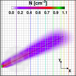
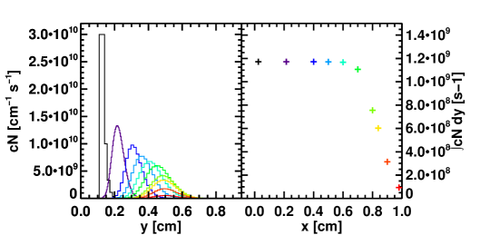
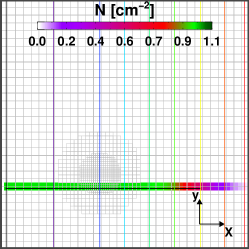
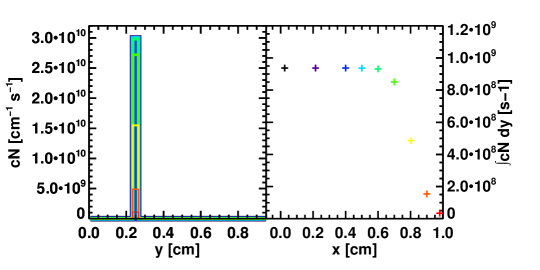
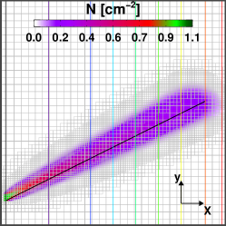
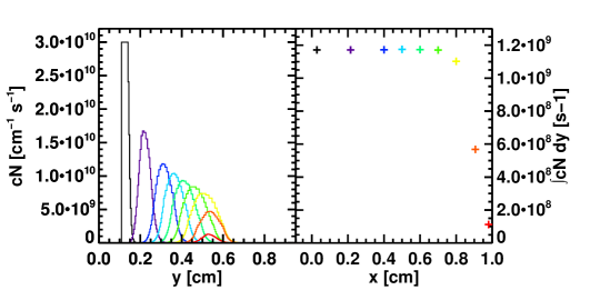
Of the seven standard RT and RHD tests described in Section 6, five include active or inactive grid refinement, demonstrating that the radiation hydrodynamics perform robustly in conjunction with (on-the-fly) cell refinements/de-refinements. In addition, we demonstrate in Fig. 7 how radiation flux is well retained across changes in grid refinement. The upper left map of the figure shows a beam of radiation in a 2D RAMSES-RT experiment, where we use the HLL flux function and deactivate radiation-gas interactions (with zero photoionization cross sections). The beam is injected into two cells in the bottom left corner by imposing a unity reduced photon flux of $3\times 10^{10}$ photons $\rm{s}^{-1}\ \rm{cm}^{-1}$, corresponding to a photon density of $1\ {\rm{cm}}^{-2}$, at an angle of $26.5^{\circ}$ from the horizontal. The beam traverses a circular region of 2 successive levels of increasing refinement, going from refinement level 6 to 8, i.e. effective resolutions of $64^{2}$ to $256^{2}$ cells. We use here straight injection (i.e. no interpolation) for inter-level cell fluxes, but linear interpolation gives identical results. The snapshot is taken at $t=3.04\times 10^{-11}$ s, just before the beam has had time to cross to the right edge of the $1$ cm wide box. To the right of the map we plot photon flux profiles, $cN$, across the coloured vertical lines in the map. The beam experiences diffusion, as can be seen by the widening of the flux profiles, but this is exclusively due to the intercell flux function and independent of the refinement changes. The far left plot shows the integrals across each flux profile, i.e. the total photon flux across each line. The values are consistent until around $x=0.6$, and then reduce to zero towards the edge of the beam. We’ve verified that if the test is let to run for double the time, i.e. about $6\times 10^{-11}$ s, the total flux is consistent throughout the whole box width to about $1$ in $10^{4}$, so photons are very well conserved across the changes in refinement.

To further demonstrate flux conservation, the lower panel in the same figure shows an identical experiment except that the beam is horizontal, such that it can be perfectly maintained with the HLL flux function. To stay just under a light crossing time, we consider a shapshot at $2.6\times 10^{-11}$ s. Here again, the flux is well preserved towards the edge of the beam, and we have verified that in two crossing times, the total flux is retained perfectly to the number precision, which here is 7 decimals.

We also consider another beam with the same setup, shown in Fig. 8, where instead of a static refinement region, the grid is actively refined on inter-cell gradients in photon density $N$. According to the criterion, two adjacent cells at positions $i$ and $i+1$ are refined if

$$2\left|\frac{N^{i}-N^{i+1}}{N^{i}+N^{i+1}+10^{-3}\ {\rm{cm}}^{-2}}\right|>0.4.$$ (43)

Straight injection (no interpolation) is used here for inter-level fluxes and cell refinements, but the results are identical when linear interpolation is used for inter-level fluxes and cell refinements. The snapshot here is taken at $3.3\times 10^{-11}$ s ($\sim$ a crossing time). The plot on the far right shows the flux conservation across different x-coordinates. (Note the total flux is slightly different from that in Fig. 7 because of the different geometry of the beam injection.) The total flux is again well maintained towards the beam edge. We verified that in two light crossing times, the discrepancy of the beam flux at different $x-$coordinates levels out to within $0.03\%$.

These simple beam experiments demonstrate that the code accurately transports radiation across (even dynamically) changing refinement levels. The main errors are the artificial diffusion of radiation on the grid, which is not caused by refinement, but rather by the inter-cell flux function, and the dipole approximation inherent to the M1 closure, which does not allow opposing streams of radiation to pass through one another. Note though that while the diffusion is artificial, the total flux is well maintained, i.e. energy is conserved.

5.3.1 Speed of light

The AMR transport tests also demonstrate that radiation in RAMSES-RT propagates at the correct speed, i.e. at the speed of light. In each beam map (Figs. 7-8), a black line has been plotted over the beam, starting at the beam injection and ending at the light-crossing distance, i.e. $t\times c$, where $t$ is the snapshot time. Qualitatively it can be seen that the beam ends roughly at the same position as the black line, and in the flux plots on the far right side of each beam map it can be seen that the beam has roughly half the original flux at this end position. The far end of the beam is smooth over a few cell widths rather than discontinuous, because of numerical diffusion.

5.4 Cosmological settings

RAMSES uses super-comoving variables to allow for the impact of the cosmological expansion on the Poisson equation, the equations of hydrodynamics (38-40) and particle propagation (Martel & Shapiro, 1998; Teyssier, 2002): a change is made from the physical variables to super-comoving ones with

$$d\tilde{t}=\frac{H_{0}}{a^{2}}\ dt,\ \ \ \ \ \ \ \ \ \ \tilde{x}=\frac{1}{aL}\ x,\ \ \ \ \ \ \ \ \ \ \tilde{\rho}=\frac{a^{3}}{\Omega_{m}\rho_{c}H_{0}^{2}}\ \rho,$$

$$\tilde{{\bf{u}}}=\frac{a}{H_{0}L}\ {\bf{u}},\ \ \ \ \ \ \ \tilde{{\varepsilon}}=\frac{a^{5}}{\Omega_{m}\rho_{c}H_{0}^{4}L^{2}}\ {\varepsilon},\ \ \ \ \ \ \ \ \ \ \ \$$

where $H_{0}$ is the Hubble constant, $\Omega_{m}$ the matter density parameter, $L$ the comoving width of the simulation box (physical width at $a=1$), and $\rho_{c}$ the critical density of the Universe. When these variables are used instead of the physical ones, the cosmological expansion is accounted for, while all relevant equations remain unchanged, Euler equations included.

For consistency, and to partly account for the effect of cosmological expansion on the radiative transfer, the additional change is made in RAMSES-RT to super-comoving RT variables for the photon transport:

$$\tilde{N}=a^{3}\ N,\ \ \ \ \ \ \ \ \tilde{{\bf{F}}}=\frac{a^{4}}{H_{0}L}\ {\bf{F}},\ \ \ \ \ \ \ \ \tilde{c}=\frac{a}{H_{0}L}\ c.$$

The dilution ($\propto a^{-3}$) of photon number density is thus accounted for, while it can easily be verified that Eqs. (6)-(7) remain unchanged with the new variables – including the reduced flux (14) used in the M1 tensor (12).

Note that when reduced light speed is used, the photons will be over-diluted in cosmological simulations, since the time taken for them to get from source to destination will be overestimated. Note also that wavelength stretching with redshift, which in reality adds a fourth power of $a$ to the dilution of $N_{\gamma}$, is not accounted for here. This is actually non-trivial to do: one could add one power of $a$ to the definitions of $\tilde{N}$ and $\tilde{{\bf{F}}}$, but it would be a very crude approximation of the wavelength dilution, as the wavelength shift that should feed photons from one group to the next is neglected. In any case, this effect is likely to be important only in the context of reionization, where the photons have a chance of travelling cosmological distances before they are absorbed. While cosmological diffusion and redshifting is difficult to account for in ray-tracing methods, where the radiation is typically traced as far as it can get in one moment in time, moment-based approach are more straightforwardly able to model these effects (e.g. Ricotti, Gnedin & Shull, 2002; Petkova & Springel, 2009; Finlator, Dave & Ozel, 2011).

6 Radiative transfer tests

The tests described in this section come from two papers that were born out of a series of workshops on radiative transfer. Tests with simple analytic results to compare to are hard to engineer in radiative transfer, so the solution was to instead make simple tests where the correct result is not necessarily well known but the results of many different codes can instead be compared. Thus it is likeliest that the correct results are usually where most of the codes agree, and if a code stands out from all or most of the others in some way, this would most likely be a problem with that particular code. These tests have become sort of benchmark tests for RT codes, and most publications that present new implementations use some or all of these tests for validation.

The first paper is Iliev et al. (2006a), hereafter known as Il06 – it describes four RT post-processing tests, i.e. with the hydrodynamic advection turned off, and shows the results for 11 RT codes. The second paper is Iliev et al. (2009), hereafter known as Il09 – it describes three additional tests, and results for 9 codes, where the RT is coupled to the hydrodynamics.

The tests results from Il06 and Il09 are normally downloadable on the web, but at the time of this writing the links have been down for some time. However, Ilian Iliev has been kind enough to provide all test results for one of the codes, the grid based short characteristics code C²-Ray, which is described in detail in Mellema et al. (2006). We thus present here RAMSES-RT results with comparisons to those of C²-Ray. The inclusion of the C²-Ray results in the plots shown here should be useful to guide the eye if one then wants to compare with the other codes in Il06 and Il09.

As prescribed by the test papers, all tests use hydrogen only gas. We use smooth RT in the RAMSES-RT runs for all tests, but remark that turning off the smoothing has no discernible effect on the results (only calculation speed). Unless noted otherwise in the following tests, the GLF intercell flux function is used (§3.2), and the the on-the-spot approximation is applied (§3.3.2). In all except test 1, where the radiation is monochromatic, the radiation energy distribution is assumed to be a $T_{\rm{eff}}=10^{5}$ K blackbody, which is approximated with three photon groups bordered by the hydrogen and helium ionization energies:

$$]13.6,\ 24.59],\ \ \ ]24.59,\ 54.42],\ \ \ ]54.42,\ \infty[\ \ \ \rm{eV}.$$ (44)

A reduced speed of light fraction of ${f_{c}}=1/100$ is used unless otherwise noted. AT08 contain an analysis of the effect of different light speeds in the first three tests from Il06, and find the results start diverging non-negligibly somewhere between ${f_{c}}=10^{-2}$ and $10^{-3}$, which matches well with our analysis in §4.2. The prescribed resolution in the tests is $128^{3}$ cells, but in most tests we use adaptive refimenent for demonstrative purposes, with a coarse resolution of $64^{3}$ cells, and an effective resolution of $128^{3}$ cells. We use a Courant factor of 0.8, so the RT timestep is set by

$$\Delta t_{\rm{RT}}=0.8\ \frac{\Delta x}{3{c_{r}}},$$ (45)

where $\Delta x$ is the cell width and ${c_{r}}$ the reduced light speed. Taking as an example the test 1 setup, which has a box width of $6.6$ kpc, a simulation time of $500$ Myr, and a reduced light speed fraction ${f_{c}}=10^{-2}$, this translates into a (fine level) timestep length of $\sim 4,500$ yr, so $\sim 10^{5}$ fine-level steps need to be computed to run the test.

6.1 Il06 test 0:    The basic thermochemistry physics

Figure 9: Il06 test 0. Single-zone photoheating and ionization with subsequent cooling and recombinations.

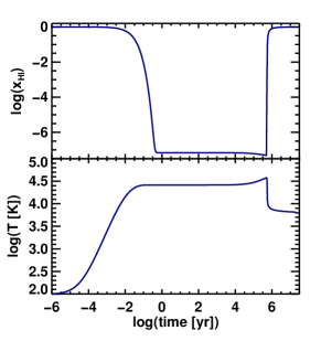
This is essentially a one-cell test of the non-equilibrium thermochemistry and not radiative transfer per se, so it doesn’t really count with the rest of the comparison project tests (hence test zero). It is important nontheless since thermochemistry is a major new component in RAMSES-RT.

We start with completely neutral hydrogen gas with density $n_{H}=1\;{\rm{cm}}^{-3}$ and temperature $T=100\;\mathrm{K}$ at $t=0$. A photo-ionizing flux of $F=10^{12}\ {\rm{s}}^{-1}\,{\rm{cm}}^{-2}$ with a $10^{5}$ K blackbody spectrum is applied to the gas and maintained until $t=0.5$ Myr at which point it is switched off. The run is continued for a further $5$ Myr, allowing the gas to cool down and recombine. The run-time is separated into 500 logarithmically equally spaced timesteps, and the thermochemistry solver sub-cycles these timesteps adaptively (see §3.3.1). The photon flux is not evolved, i.e. it is kept fixed (until $0.5$ Myr) thoughout the integration. The resulting evolution of the neutral fraction and temperature of the gas is shown in Fig. 9. The evolution closely follows that of the codes described in Il06, with the exception of SimpleX and FFTE which stand out somewhat, and we don’t see any sign of the stiffness-induced oscillations that can be seen in the Crash code test.

6.2 Il06 test 1:    Pure hydrogen isothermal HII region expansion

A steady monochromatic ($h\nu=13.6$ eV) source of radiation is turned on in a homogeneous neutral gas medium, and we follow the resulting expansion of a so-called Strömgren sphere of ionized gas. Heating and cooling is turned off and the temperature is set to stay fixed at $T=10^{4}$ K.

The box is a cube of width $L_{box}=6.6$ kpc. The gas density is $n_{\rm{H}}=10^{-3}\,{\rm{cm}}^{-3}$ and the initial ionization fraction is $x_{\rm{H\scriptscriptstyle I}}=1.2\times 10^{-3}$, corresponding to collisional ionization equilibrium. The radiative source is in the corner of the box and the emission rate is $\dot{N}_{\gamma}=5\times 10^{48}\,\rm{photons}\;\rm{s}^{-1}$. The simulation time is $t_{sim}=500$ Myr. To demonstrate on-the-fly AMR at work (and speed up the runtime), we use a base resolution of $64^{3}$ cells, but allow for one level of further refinement, i.e. to the effective prescribed resolution of $128^{3}$ cells. Typically, AMR refinement is applied on mass-related criteria, since massive structures are usually the objects of interest in simulations. However, since the density field is homogeneous in this test, we apply refinement on gradients in $x_{\rm{H\scriptscriptstyle I}}$ and $x_{\rm{H\scriptscriptstyle II}}$: two adjacent cells at positions $i$ and $i+1$ are refined if

$$2\left|\frac{x^{i}-x^{i+1}}{x^{i}+x^{i+1}}\right|>0.8,$$ (46)

where $x$ is either $x_{\rm{H\scriptscriptstyle I}}$ or $x_{\rm{H\scriptscriptstyle II}}$.

Figure 10: Il06 test 1. Map of the neutral fraction in a box slice at $z=0$, at $500$ Myr. Overplotted is the AMR grid, which is refined on the fly during the experiment from $64^{3}$ to $128^{3}$ cells effective resolution. Maximum refinement stays on the corner source throughout the run, and it adaptively follows the expansion of the I-front.

(a)

(b)

(c)

Figure 11: Il06 test 1. (a) Evolution of the I-front position and velocity. Blue solid lines show our result, red dashed lines show the C²-Ray result and green dot-dashed lines show the analytic expression. (b) Spherically averaged profiles for neutral fractions $x_{\rm{H\scriptscriptstyle I}}$ and ionized fractions $x_{\rm{H\scriptscriptstyle II}}$ at $30$ and $500$ Myr versus radius (in units of the box width $L_{\rm{box}}$). (c) Histogram showing fractions of cells within bins of $x_{\rm{H\scriptscriptstyle I}}$ at three simulation times.

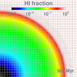
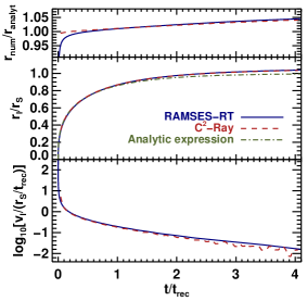
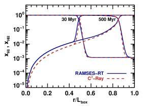
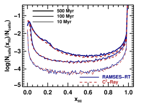
The Strömgren radius, $r_{\rm{S}}$, is the radius of the ionization front (I-front) from the center when steady state has been reached, and in the case of fixed density and temperature it has the simple analytical result shown in Eq. 32. In this result the I-front evolves in time according to

$$r_{\rm{I}}=r_{\rm{S}}\left[1-e^{-t/t_{\rm{rec}}}\right]^{1/3},$$ (47)

where $t_{\rm{rec}}=(n_{\rm{H}}\alpha^{\rm{B}}_{\rm{H\scriptscriptstyle II}})^{-1}$ is the recombination time. For the parameters of this experiment, $t_{\rm{rec}}=122.4$ Myr and $r_{\rm{S}}=5.4$ kpc.

Fig. 10 shows maps at $500$ Myr of the neutral fraction, with the grid refinement overplotted, in a box slice at $z=0$. The Strömgren sphere is nicely symmetric and qualitatively it can be seen to agree well with results from the RT codes described in Il06 (their Fig. 6).

Fig. 11a shows the evolution of the I-front position and velocity with RAMSES-RT (solid blue), compared with the analytic expression (green dot-dashed) and the result for the C²-Ray code (red dashed), which is typical for the RT code results presented in Il06 and does not stand out particularly in this test. Our result can be seen to match the C²-Ray one, though we have an initial lag due to the reduced speed of light that can best be seen in the top plot showing the fraction of the numerical result’s I-front radius versus $r_{\rm{S}}$. The analytic $r_{\rm{I}}$ is typically ahead of $r_{\rm{S}}$ by $\la 5\%$, which is simply because the analytic result is step-like with complete ionization within $r_{\rm{S}}$ and none outside, whereas the real result has a gradually evolving ionization profile with radius. Indeed, Pawlik & Schaye (2008) computed the exact analytic result to this problem, accounting for an equilibrium neutral fraction inside the Strömgren sphere, and found an equilibrium I-front radius which is exactly $1.05\ r_{\rm{S}}$.

Fig. 11b shows spherically averaged radial profiles of the gas ionization state at $30$ and $500$ Myr. Again we see a good match with the C²-Ray result. There is still a little lag in the I-front position at $30$ Myr due to the RSLA and $x_{\rm{H\scriptscriptstyle I}}$ is somewhat lower inside the Strömgren sphere in RAMSES-RT. However, the C²-Ray result stands out a little in this test in Il06 as being most effective at ionizing the gas within the Strömgren sphere (i.e. has the lowest values of $x_{\rm{H\scriptscriptstyle I}}$), and the RAMSES-RT result is typical of the Il06 codes’ results in this plot.

Figure 12: Il06 test 1. Evolution of the globally averaged neutral fraction.

(a)

(b)

(c)

(d)

Figure 13: Il06 test 2. Maps showing slices at $z=0$ of the neutral fraction and temperature at 10 Myr and 100 Myr.

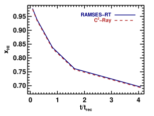
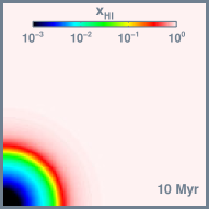
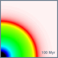
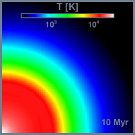
A further comparison is made in Fig. 11c, here comparing ionization fraction histograms at three simulation times. Again the RAMSES-RT result closely matches the C²-Ray one, whose histograms fall into a group with the codes IFT, Flash-HC and FFTE that stand out a little in Il06 (Fig. 9) as having less frequent intermediate neutral fractions than the other codes.

Finally for this test, Fig. 12 shows a comparison with C²-Ray of the globally averaged neutral fraction as a function of time. It is a close match, and the C²-Ray result is here typical for the Il06 codes.

All in all, there is nothing out of the ordinary in the RAMSES-RT result for Il06 test 1, except for a slight initial delay of the I-front which is to be expected due to the RSLA.

We note that performing this test with the full prescribed $128^{3}$ resolution, rather than using AMR like we’ve done here, has no discernible effect on the results. In the AMR run, the number of fine level cells is maximally (at the end of the run) $15\%$ of the number of fine level cells in the non-AMR run, and the computation time is $~{}30\%$ of that in the non-AMR run. The cost of the experiment (with AMR) is on the order of 50 cpu hours, which is a lot for a simple test in which little actually happens: for much of the run, the I-front is moving towards a stand-still at speeds which are much slower than our reduced speed of light (${f_{c}}=0.01$), so barring the RT Courant condition, the timesteps taken could have dramatically increasing length towards the end of the test. Implicit transport solvers can take advantage of this (almost) static situation by on-the-fly adapting the timestep length (which is in the case of implicit solvers not constrained by the Courant condition), so presumably an implicit solver can run this test (and most of the tests described in this work) with considerably less computation than we do. However, in more realistic cosmological scenarios, such steady regimes simply do not happen over times longer than the typical age of stellar populations, which is on the order of $10$ Myr ($50$ times shorter than the run-time for this test). Furthermore, stellar populations typically are turning on and off on even shorter timescales than that thoughout the simulation volume, which limits the dynamical time of ionization fronts even further. This presumably constrains the main advantage (possible long time steps) of implicit solvers severely, since even though they are not constrained by Courant-like conditions, they still need to resolve dynamical timescales.

(a)

(b)

(c)

Figure 14: Il06 test 2. (a) Evolution of the temperature and ionization state profiles. (b) Evolution of the ionization front. The top plot shows the ratio of the radius of the I-front in the tests, $r_{\rm{num}}$ versus the time-evolving radius $r_{\rm{analyt}}$ in the analytic result from test 1 (Eq. 47). The middle plot shows the ratio of the test I-front radius versus the steady-state radius in the same analytic result (Eq. 32). The bottom plot shows the speed of the I-front, $v_{\rm{I}}$ in units of a ‘characteristic’ speed, given by $r_{\rm{S}}/t_{\rm{rec}}$. (c) Histograms of temperature and ionized fraction.

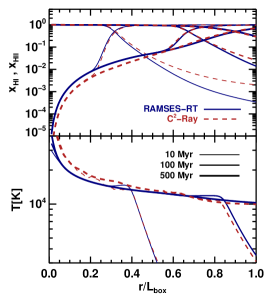
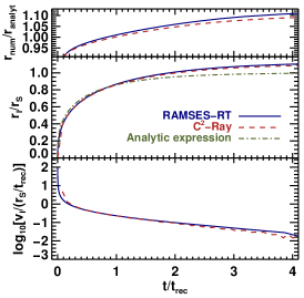
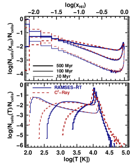
6.3 Il06 test 2:   HII region expansion and the temperature state

The setup here is the same as in Il06 test 1, except for the following points:

• We allow for cooling and photo-heating of the gas, i.e. the temperature is no longer constant, and the analytic result, Eq. 32 no longer applies (because of the non-constant recombination rate).

• The initial temperature is $100$ K.

• The initial ionization fraction of the gas is $x_{\rm{H\scriptscriptstyle II}}=10^{-6}$. It should be fully neutral according to the test recipe in Il06, but this is (the default) minimum value for $x_{\rm{H\scriptscriptstyle II}}$ in RAMSES-RT, that exists in order to keep bounds on the subcycling of the thermochemistry. In any case, the specific value is not critical to the test results, as long as it is low.

• The radiation source is a $T=10^{5}$ K blackbody, modeled with the three photon groups defined by (44). The emission rate is the same as before, $\dot{N}_{\gamma}=5\times 10^{48}\,\rm{photons}\;\rm{s}^{-1}$.

• We don’t use grid refinement in this test. The grid is homogeneous and the resolution is $128^{3}$ grid cells, as prescribed in Il06.

Slice maps at $z=0$ of the neutral fraction and temperature are shown in Fig. 13. Both the ionization and heating fronts are smooth and symmetric, and the maps agree qualitatively with other codes in Il06 (Figs. 11-14). In comparison with the same test with ATON (AT08, Fig. 3), both fronts are clearly much thicker here, which is due to our multi-frequency implementation (whereas ATON used one photon group). More detailed comparison with the Il06 codes can be made through the ionization state and temperature plots in Fig. 14a, where we include the C²-Ray result. The ionization state profile develops very similarly to that of C²-Ray, though we have less ionization on both sides of the front, especially on the outer side where the difference in $x_{\rm{H\scriptscriptstyle II}}$ is as high as a factor of ten. Presumably this is due to the different implementations of multi-frequency photo-heating and cooling. The thermal profiles are also similar to C²-Ray, though we have considerably lower (up to a factor of two) temperatures on the inside of the I-front, and conversely higher temperatures on the outside. As can be seen in Fig. 17 in Il06, C²-Ray has the strongest heating of any code on the inside of the I-front in this test and most codes have stronger heating on the outside, so our thermal profiles (as the ionization state profiles) are fairly typical of the ones presented in Il06 for this test.

Fig. 14b shows the evolution with time of the ionization front, compared with C²-Ray and the analytic result from test 1. The front moves more slowly here than in test 1 due to the lower initial temperature, so we no longer lag behind in the initial front propagation. Our front propagates slightly further than in C²-Ray, and ends at almost exactly the same radius as the FFTE code, which has the furthest expanding I-front of any code in this test in Il06. Still the difference between the codes is small, with the ratio between the numerical and analytic results ($r_{\rm{num}}/r_{\rm{analyt}}$) ranging between $1.01$ and $1.11$.

Fig. 14c shows histograms of the ionized fraction and temperature at different times in the test for RAMSES-RT and C²-Ray. The ionized fraction histograms are quite similar, the biggest difference being a higher fraction of almost completely neutral gas $x_{\rm{H\scriptscriptstyle II}}\la 10^{-2}$ in RAMSES-RT, which we already saw in Fig. 14a (top) beyond the I-front. The temperature histogram for RAMSES-RT differs a bit from C²-Ray in having less extreme temperatures (C²-Ray has both hotter gas and colder gas) but are very similar to those for the codes ART, RSPH and Crash in Il06.

Finally, Fig. 15 shows the time evolution of the volume averaged neutral fraction in RAMSES-RT and C²-Ray, and here we see a close match. There is quite a lot of discrepancy between the different codes in the analogue plot in Il06 (Fig. 20), with 3 groups of results, and our result closely follows those of C²-Ray, Crash and RSPH.

As with test 1, there is nothing out of the ordinary in the RAMSES-RT result for Il06 test 2, except perhaps for an ever so slightly further advanced I-front than most codes in Il06 have.

Figure 15: Il06 test 2. Time evolution of the volume average neutral fraction.

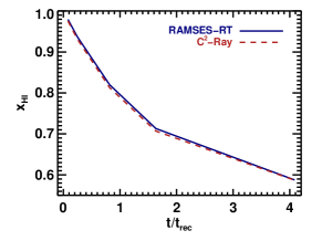
6.4 Il06 test 3:   I-front trapping in a dense clump and the formation of a shadow

(a)

(b)

(c)

(d)

(e)

(f)

(g)

(h)

(i)

(j)

(k)

(l)

(m)

(n)

(o)

(p)

(q)

Figure 16: Il06 test 3. Maps showing slices at $z=0.5\ L_{\rm{box}}$. The top map shows the (constant) density field, with the static refinement overplotted. The second row shows the RAMSES-RT+HLL results in terms of neutral fraction (left) and temperature (right) at 1 and 15 Myr. The third row Shows the RAMSES-RT+HLL results without the on-the-spot approximation. The fourth row shows the RAMSES-RT+GLF results. The bottom row shows the C²-Ray results for comparison.

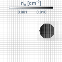
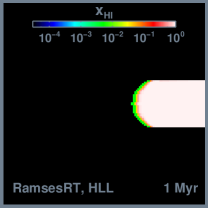
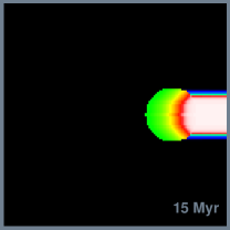
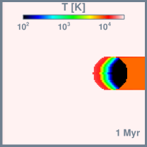
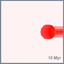
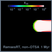
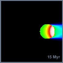
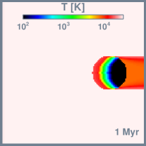
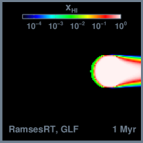
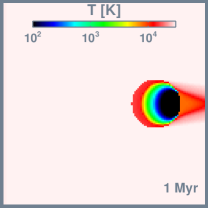
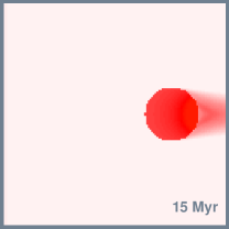
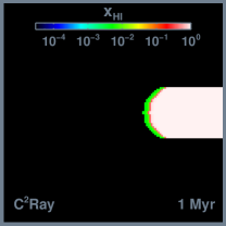
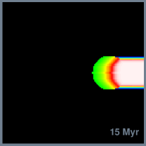
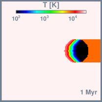
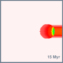
This test considers self-shielding within a dense gas cloud bombarded on one side by UV radiation, and the shadow trailing on the ‘dark’ side - something which may find place with clouds close to sites of star-formation.

The setup is as follows: the simulation box has width $L_{\rm{box}}=6.6$ kpc. We place a spherical cloud of gas in the center of the ($y,z$)-plane, with radius $r_{\rm{cloud}}=0.8$ kpc, and it’s center at $(x_{c},y_{c},z_{c})=(5,3.3,3.3)$, as seen in Fig. 16, top left, showing an $(x,y)-$slice of gas density through the middle of the box. Outside the gas cloud we have $n_{\rm{H}}^{\rm{out}}=2\times 10^{-4}\,{\rm{cm}}^{-3}$, $T^{\rm{out}}=8000$ K and $x_{\rm{H\scriptscriptstyle II}}^{\rm{out}}=0$, and inside we have $n_{\rm{H}}^{\rm{cloud}}=200\,n_{\rm{H}}^{\rm{out}}=4\times 10^{-2}\,{\rm{cm}}^{-3}$, $T^{\rm{cloud}}=40$ K and $x_{\rm{H\scriptscriptstyle II}}^{\rm{cloud}}=10^{-6}$. We apply a constant ionizing photon flux $F=10^{6}\;{\rm{s}}^{-1}\,{\rm{cm}}^{-2}$ from the $x=0$ boundary of the box (left in the Fig. 16 maps), and run for $15$ Myr. We use a light speed fraction of ${f_{c}}=10^{-1}$. This is ten times higher than the “norm” in the RT tests, but it is needed for the light to have reached the cloud in the first snapshot under consideration, at 1 Myr. In order to best capture the formation of a shadow behind the cloud, we apply the HLL flux function in this test rather than the usual GLF function, and we use the OTSA. We have run identical tests though, one with the GLF flux function, and one where we use the HLL flux function but don’t assume the OTSA, and we show maps of those experiments for a qualitative comparison. As usual, the resolution prescribed by Il06 is $128^{3}$ cells, but here we apply static AMR refinement such that the coarse resolution is $64^{3}$ cells, but a rectangular region that encompasses the gas cloud and the shadow behind it has one level of additional refinement, making the effective resolution in the cloud and its shadow $128^{3}$ cells. The refinement region is shown in the top panel of Fig. 16, plotted over a density map that shows the spherical gas cloud. The fraction of volume at the fine resolution is $4\%$, and the computation time for the test is roughly a quarter of a an analogous uniform grid run (about $32/130$ cpu hours for the AMR/non-AMR runs).

(a)

(b)

(c)

Figure 17: Il06 test 3: RAMSES-RT+HLL versus C²-Ray comparinson. (a) Evolution of the position and speed of the I-front along the x-axis through the center of the box. The position plot (top) shows the x-position where $x_{\rm{H\scriptscriptstyle II}}=0.5$, with respect to the center of the cloud, $x_{C}=5$ kpc, in units of the Strömgren length inside the cloud, $\ell_{S,cl}=0.78$ kpc. The dotted horizontal lines mark the edges of the cloud. The speed (bottom) is plotted in units of twice the isothermal sound speed in the cloud at $T=10^{4}$ K, $2c_{s,l}(10^{4}\,\mathrm{K})=2.35\times 10^{6}$ cm/s. (b) Evolution of the average ionized fraction (top) and temperature (bottom) inside the dense cloud. (c) Profiles along the x-axis through the box center of the ionization state (top) and temperature (bottom), at 1, 3 and 15 Myr.

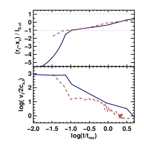
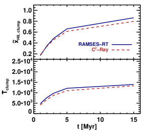
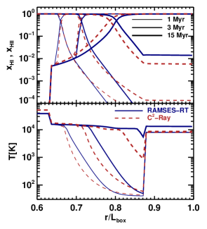
Fig. 16 shows slices at $z=0.5\ L_{\rm{box}}$ of the neutral fraction and temperature at $1$ and $15$ Myr. From second top to bottom row are shown RAMSES-RT+HLL, RAMSES-RT+HLL without the OTSA, RAMSES-RT+GLF (with the OTSA) and C²-Ray. The I-front travels fast through the diffuse medium outside the cloud, but moves much more slowly inside it, and a shadow is cast behind it. As the UV radiation eats its way into the cloud, ionizing and heating it, the shadow also very slowly diminishes in width because some photons manage to cross through the edges of the cloud. The RAMSES-RT+HLL maps compare very well with C²-Ray, though the shadow is slightly thinner at $15$ Myr and there is stronger heating inside the shadow; this could be due to differences in the multifrequency approach and/or photoheating. Without the OTSA, the shadow is diminished from the sides due to photons being cast from the surrounding gas. Using the GLF flux function has much the same effect as not assuming the OTSA, though the shadow is considerably more diminished here. The result with HLL but without the OTSA is the most physical of the RAMSES-RT results, as one should expect recombination photons to be cast into the shadow.

Fig. 17a shows the evolution of the position and speed of the I-front through the center of the $(y,z)-$plane. In solid blue we plot the RAMSES-RT result and in dashed red is the C²-Ray result for comparison. Horizontal dotted lines mark the edges of the cloud. There is a large initial delay in the I-front compared to C²-Ray, which is because in the diffuse gas outside the cloud, the I-front speed is limited by the reduced speed of light. After the I-front gets into the cloud (lower dotted line) it quickly catches up and then evolves in a similar fashion in the two codes. If compared to the rest of the codes in Il06, it turns out that the evolution of the I-front in C²-Ray slightly stands out from the rest of the codes (e.g. a small upwards ‘bump’ in the front position at $log(t/t_{\rm{rec}})\sim 0$, and a slightly shorter distance of the I-front from the origin at the end of the simulations), and most of the others in fact evolve very similarly to that of RAMSES-RT. The comparison appears best with RSPH, which has the furthest extended I-front at the end-time of $15$ Myr. The same can be said for the speed of the front. If we look away from the initial $\sim 0.2$ Myr, when our I-front has to catch up, the speed compares reasonably to C²-Ray, and quite well to the other codes in Il06.

Fig. 17b shows the evolution of the mean ionized fraction and temperature inside the cloud, compared between RAMSES-RT and C²-Ray. The evolution is similar between the two codes in both cases. Compared with the other codes in Il06, the evolution of the ionized fraction is most similar to RSPH, IFT and Coral, while the temperature in RAMSES-RT is consistently a little higher than in most codes (all except Coral and Flash which stand out quite a lot in mean temperature).

Figure 18: Il06 test 3: RAMSES-RT+HLL versus C²-Ray comparison. Histograms of neutral fraction (top row) and temperature (bottom) inside the dense cloud at 1, 3 and 15 Myr (from left to right).

Fig. 17c shows profiles of the ionization state and temperature along the x-axis at the center of the $(y,z)-$plane at $1$, $3$ and $15$ Myr. The ionization state profile in RAMSES-RT is similar in most respects to that of C²-Ray, though it extends a bit further at the end of the run-time. There is initially less ionization on the far side of the front in RAMSES-RT, but at the end of the run this is reversed and we have slightly more ionization on the far side in RAMSES-RT. This ‘shift‘ can be explained by the temperature profiles: at early times the cloud is efficiently shielding the far side from even the high-energy photons in both codes, but at the end of the RAMSES-RT run the shielding buffer in the cloud is thin enough that the high-energy photons can get through, hence efficiently heating the gas inside the buffer as well as in the shadow, and the gas in the shadow becomes slightly ionized as a consequence. The analogue ionization state profiles for the other codes in Il06 are mostly similar to ours. Most of them are actually closer to the RAMSES-RT than the C²-Ray profile, with the exception of Crash which has a much more underdeveloped I-front and less ionization, and FFTE and IFT which have an almost step-wise $x_{\rm{H\scriptscriptstyle II}}$-profile on the far side of the I-front. The temperature profiles differ pretty widely between the codes. RAMSES-RT doesn’t particularly stand out, though, and is most similar to that of Coral at $15$ Myr. The temperature profile for RAMSES-RT also differs notably from that of ATON, where the shielded region inside the cloud is thicker and more step-like both in the ionized fraction and temperature, due to the monochromatic radiation.

Finally, Fig. 18 shows histograms of the neutral fraction and temperature at $1$, $3$ and $15$ Myr for RAMSES-RT and C²-Ray. The comparison (also with the other codes in Il06) is qualitatively similar, though there is quite a difference between the individual codes in these plots.

As with the previous tests, RAMSES-RT performs well here and we don’t really have anything out of the ordinary in our results. One should keep in note though that here we’ve used the non-diffusive HLL flux function, whereas in most cosmological simulations it would be more natural to use the more diffusive GLF function to have better spherical symmetry around radiative stellar sources, which comes with the price of less pronounced and shorter lived shadows than HLL. The survival of shadows in more realistic scenarios remains an open question, but considering the effects of recombination radiation, and the likelihood of any transparent region to have ionizing sources shining from different directions, it seems unlikely to us that shadowing is an efficient way of shielding gas from ionizing radiation.

6.5 Il06 test 4:   Multiple sources in a cosmological density field

This test involves the propagation of ionization fronts in a static hydrogen-only density field taken from a cosmological simulation snapshot at redshift 9. The density cube is $128^{3}$ cells and its width is $500\,h^{-1}$ co-moving kpc (corresponding to $50\,h^{-1}$ physical kpc). The Hubble factor is $h=0.7$. The initial temperature is fixed at $100$ K everywhere. 16 radiative sources are picked out corresponding to the most massive halos in the box and these are set to radiate continuously for $0.4$ Myrs. The mass-dependent radiation intensity for each halo is given in a downloadable table (from the RT comparison project website). Unlike in Il06, we don’t apply the OTSA in this test, i.e. we include the radiative transfer of recombination radiation, but we’ve verified that this has no discernible effect on the results. Our analysis from §4.2 indicates that a reduced light speed gives incorrect results in this test. Thus we use a full light speed here (i.e. $f_{c}=1$), and for comparison with the codes from Il06, which implicitly assume infinite light speed, we make an analogue run with a hundred-fold light speed ($f_{c}=100$).

(a)

(b)

(c)

(d)

(e)

(f)

(g)

(h)

(i)

(j)

(k)

(l)

Figure 19: Il06 test 4. Maps showing slices at $z=0.5\ L_{\rm{box}}$ of the neutral fraction and temperature at times 0.05 Myr and 0.4 Myr. Top row shows RAMSES-RT results with physical light speed. The middle row shows the C²-Ray results (infinite light speed). The bottom row shows the RAMSES-RT results with one hundred times the physical light speed.

(a)

(b)

Figure 20: Il06 test 4. (a) Time evolution of the mass weighted and volume weighted average ionized fractions. (b) Histograms of neutral fraction (top) and temperature (bottom).

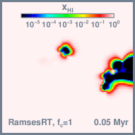
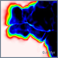
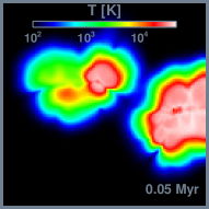
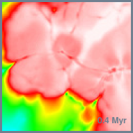
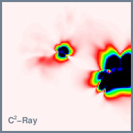
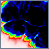
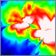
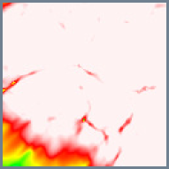
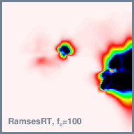
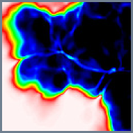
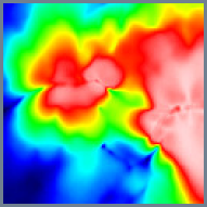
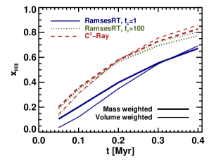
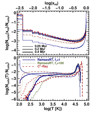
Fig. 19 shows box slices, at $z=0.5\ L_{\rm{box}}$, of the neutral fraction and temperature at times $0.05$ and $0.4$ Myr. Shown are our two runs with different light speed fractions (top and bottom row), and for comparison we show the result for the C²-Ray code, from Il06: the I-fronts and photo-heating in our $f_{c}=1$ run clearly lag behind the C²-Ray result, and there is also less heating of the ionized gas. This is in accordance with the ATON results described in AT08, where a similar delay was found. They prescribed this delay to the fact that ATON is monochromatic, but since our multi-frequency approximation (three photon groups) gives results that are still much more similar to the ATON results than those of C²-Ray, especially in terms of the neutral fraction maps, we are inclined to blame the delay on another factor, which is the speed of light. Our results with the speed of light set to one-hundred times the physical value are shown in the bottom row of Fig. 19 and here the results are considerably closer to those of C²-Ray in terms of the propagation of heating- and I-fronts, although the maximum temperature in the ionized gas is still colder in comparison. All four codes considered in the Il06 4 test use an infinite effective speed of light and this may give premature fronts in the immediate vicinity of the sources and also further away in under-dense regions. Thus we are perhaps not really dealing with a delay in RAMSES-RT, but rather premature fronts in the Il06 codes. As AT08 note, we are far from reaching a static state in the fronts in this experiment in the run-time of $0.4$ Myr and we should expect the different light speed runs to converge to similar results when static state is reached. This is further corroborated by our I-front light crossing time analysis from Section 4.2.

The smaller degree of photo-heating in the ionized gas compared to the C²-Ray results is in line with the temperature profiles from the previous tests (e.g. Fig. 14a), and presumably is a consequence of the different ways multi-frequency is approximated. Another notable difference in the maps in Fig. 19 is that our fronts are smoother and less jagged than those in C²-Ray. This is an effect of the photon diffusion inherent in the GLF flux function used here. Like AT08 we find that using HLL instead gives more jagged fronts.

Fig. 20a shows the evolution of the mass- and volume-weighted ionized fractions, compared for the different runs. The RAMSES-RT run with the physical light speed gives ionized fractions which are close (both mass- and volume-weighted) to the ATON ones, whereas increasing the light speed by a factor of hundred from the physical value gives results closer to C²-Ray (as well as the three other codes that ran this test in Il06). Presumably we would converge further towards C²-Ray in the limit of infinite light speed, but computational time constraints do not allow to pursue that investigation. This is a further hint that the correct speed of light is important in the non-steady regime of ionization fronts.

Finally, Fig. 20b shows neutral fraction and temperature histograms at three times in the test. Again there is a strong discrepancy between the RAMSES-RT run with $f_{c}=1$ and C²-Ray, especially at early times, and the gap all but closes when $f_{c}=100$ is used instead with RAMSES-RT. There remains some difference though in the minimum/maximum temperature, being smaller/larger for C²-Ray than for our $f_{c}=100$ run, presumably because of our rather crude multi-frequency approximation.

To summarize, there is notable discrepancy between the RAMSES-RT results and those presented in Il06, in that the RAMSES-RT ionization front lags behind, which appears to be due to a finite speed of light. This is corroborated to some degree by other papers in the literature: Wise & Abel (2011) use a finite light speed and seem to get results which are slightly lagging as well. Pawlik & Schaye (2008) specifically do a comparison between finite and infinite light speed, with the finite one resulting in a delay which is substantial, though maybe a bit less than ours, and they do comment on the ionization bubbles in this test being unphysically large with infinite light speed methods. Other sources appear to be in conflict with our conclusions, though: Petkova & Springel (2011a) use a finite light speed and get results which seem to compare well with those of C²-Ray.

(a)

(b)

(c)

(d)

(e)

(f)

(g)

(h)

(i)

(j)

(k)

(l)

(m)

(n)

(o)

(p)

(q)

(r)

Figure 21: Il09 test 5. Maps showing slices at $z=0$ of various quantities at 100 Myrs (top panel) and 500 Myrs (lower panel). In each panel, the top row shows the RAMSES-RT results and the lower row shows the Capreole+C²-Ray results for comparison.

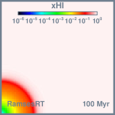
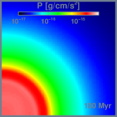
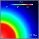
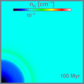
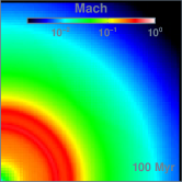
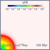
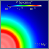
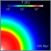
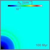
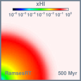
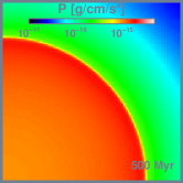
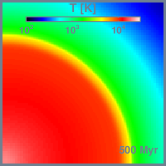
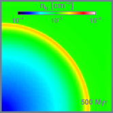
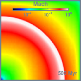
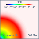
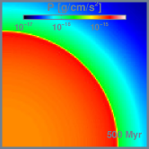
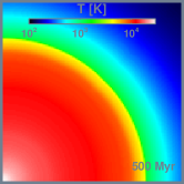
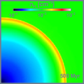
6.6 Il09 test 5:   Classical HII region expansion

We now come to the tests described in second radiative transfer codes comparison paper by Iliev et al. (2009), which we denote as Il09. This paper provides 3 code comparison tests to add to those in Il06, but with the important difference that whereas the Il06 tests are pure radiative transfer post-processing tests with fixed density fields, the tests in Il09 are RHD tests, i.e. with the radiative transfer directly coupled to the gas-dynamics. Thus we now switch from the context of post-processing RT to hydro-coupled RHD. Here, the pressure buildup in photo-heated gas causes it to expand. Typically, the I-front is initially R-type, where it expands much faster than the gas response to it, which means RT-postprocessing is a fairly good approximation. The I-front then begins to slow down when it approaches the Strömgren radius, but gets moving again when the gas catches up to it, and then the front is D-type, i.e. moves along with the expanding gas.

Figure 22: Il09 test 5. Radial profiles at 10, 200 and 500 Myrs, compared to the Capreole+C²-Ray results. Clockwise from top left: ionization fractions, pressure, temperature, Mach number, atom number density.

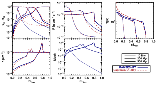
As before we compare our RAMSES-RT tests results with those of the grid-based short characteristics ray-tracing code C²-Ray (Mellema et al., 2006), here coupled to the Capreole code, which employs a Riemann solver for the hydrodynamics. As the Capreole+C²-Ray combination is sensitive to numerical instabilities appearing in Il09 test 6, we compare also in that particular test to C²-Ray coupled to the Eulerian TVD solver of Trac & Pen (2004) (that combination was not used in any other tests). The test numbers continue from the Il06 paper, thus we now come to Il09 test 5, which concerns the expansion of an ionization front due to a point source in an initially uniform-density medium. The initial setup, much like that of Il06 test 2, is as follows.

The box cube is $L_{\rm{box}}=15$ kpc in width. The gas is hydrogen only as usual, initially homogeneous with density $n_{\rm{H}}=10^{-3}\,{\rm{cm}}^{-3}$, temperature $100$ K, and ionization fraction $x_{\rm{H\scriptscriptstyle I}}=10^{-6}$ (Il09 prescribes $x_{\rm{H\scriptscriptstyle I}}=0$). The radiative source is in the corner of the box and the emission rate is $\dot{N}_{\gamma}=5\times 10^{48}\,\rm{photons}\;\rm{s}^{-1}$. We don’t apply the OTSA in this test, i.e photons are emitted from gas recombinations. The simulation time is $500$ Myr. The base resolution of the box is $64^{3}$ cells and we apply on-the-fly refinement on $n_{\rm{H}}$ and $x_{\rm{H\scriptscriptstyle II}}$ gradients (see Eq. 46), so that the ionization front has the prescribed effective resolution of $128^{3}$ cells.

We first compare volume dissections at $z=0$ in the simulation cubes at $100$ and $500$ Myr, for the RAMSES-RT and C²-Ray results, shown in Fig. 21. The maps show, from left to right, the neutral fraction, pressure, temperature, density and mach number, $M\equiv v/c_{S}$, where $c_{s}=\sqrt{1.4\ P/\rho}$ is the sound speed. (Unfortunately the $M$ output is missing from the C²-Ray results we’ve downloaded.) In these maps, the RAMSES-RT results look very similar to those of C²-Ray. The $x_{\rm{H\scriptscriptstyle I}}$-maps show stronger ionization immediately around the corner source in the C²-Ray result, and correspondingly the temperature and density maps show this corner gas is also hotter and more diffuse in the C²-Ray result than in RAMSES-RT. Conversely, the photo-heating region is somewhat further-reaching in the RAMSES-RT result than in C²-Ray, as can be seen in the pressure and temperature maps. These small differences are likely due to the different approaches in approximating multi-frequency. Notably, the C²-Ray maps stand out in a very similar way when compared to most of the corresponding maps from other codes in Il09, i.e. a stronger effect close to the radiative source but shorter-reaching photo-heating.

To paint a more quantitative picture, Fig. 22 compares radial profiles of the same quantities ($x_{\rm{H\scriptscriptstyle I}}$, $P$, $T$, $n_{\rm{H}}$ and $M$) for RAMSES-RT and C²-Ray at $10$, $200$ and $500$ Myr. The ionization state profiles (top left) indeed show C²-Ray to ionize the gas more strongly close to the radiative source, but RAMSES-RT to ionize more strongly beyond the I-front. The I-front itself is however at very similar positions at all times. The pressure and temperature plots show the same thing, but apart from these minor differences at the extreme ends the shapes are very similar. The density plots show that C²-Ray has more has more diffuse gas close to the source as a result of the stronger photoheating, and also it appears to have a more pronounced backflow peak around $200$ Myr (this double peak is a temporary effect of photo-heating by high-energy photons beyond the I-front). The smaller backflow peak in RAMSES-RT is perhaps in part a relic of on-the-fly refinement, though most of the codes in Il09 actually have backflow peaks similarly smaller than that of C²-Ray. Unfortunately we can’t compare the Mach profiles directly, but the RAMSES-RT profiles do look very similar in shape to those presented in Il09 (see their Fig. 15).

Figure 23: Il09 test 5: Time evolution of the ionization front, compared to the results from the Capreole+C²-Ray combination. Upper plot shows the radius of the Strömgren sphere in units of 5.4 kpc. The lower plot shows the speed of the front propagation.

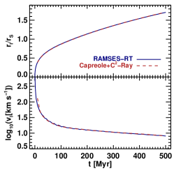
Finally, Fig. 23 shows how the position and velocity of the I-front (defined as where the radial average of $x_{\rm{H\scriptscriptstyle II}}$ is equal to 0.5), for RAMSES-RT and C²-Ray. The plots for the two codes are virtually identical, the only noticeable difference being a slight initial lag in the front speed. One might attribute this to the reduced speed of light in the RAMSES-RT run, but actually most other codes described in Il09 have a very similar lag in the initial front speed compared to C²-Ray.

The fraction of the volume refined to the effective resolution of $128^{3}$ cells is $28\%$ at the end of the run, and the computational time is roughly half that of an analogous uniform grid run. The runs clock in at about double the cpu hours of test 1, even though test 1 had roughly twice the number of timesteps to perform, due to a smaller box width. This gives a qualitative idea of the added cost of adding two more photon groups (test 1 had one group) and coupling with the hydrodynamics, which totals to about four times the computational load.

All in all, the RAMSES-RT results for this test compare very well with most of the codes presented in Il09. The RAMSES-RT result differs slightly from that of C²-Ray in some aspects, most notably in the form of weaker photo-heating and ionization close to the radiative source and wider I-fronts. However, these are precisely the aspects where C²-Ray stands out from the other codes presented in Il09.

6.7 Il09 test 6:   HII region expansion in a $\mathbf{r^{-2}}$ density profile

This test mimics a radiative source going off in a dense cloud, e.g. a stellar nursery. The setup is much like that of the preceding test 5, the main difference being that the gas is here inhomogeneous, the box is much smaller, $L_{\rm{box}}=0.8$ kpc in width, and the radiative corner source is a hundred times more luminous, i.e. it radiates at $\dot{N}_{\gamma}=5\times 10^{50}\,\rm{photons}\;\rm{s}^{-1}$. As in the previous test we don’t apply the OTSA. The base resolution is $64^{3}$ cells, but on-the-fly refinement on $n_{\rm{H}}$ and $x_{\rm{H\scriptscriptstyle II}}$ gradients ensures the prescribed effective resolution of $128^{3}$ cells at ionization and shock fronts. The initial temperature is $100$ K everywhere and the running time is $75$ Myr. The dense cloud is centered on the corner source and is set up with a spherically symmetric, steeply decreasing power-law density profile with a small flat central core of gas number density $n_{0}=3.2$ ${\rm{cm}}^{-3}$ and radius $r_{0}=91.5$ pc:

$$n_{\rm{H}}(r)=\begin{cases}\;n_{0}&\mathrm{if}\,r\leq r_{0}\\ \;n_{0}(r_{0}/r)^{2}&\mathrm{if}\,r\geq r_{0}.\end{cases}$$ (48)

Figure 24: Il09 test 6: time evolution of the ionization front, compared to the Capreole+C²-Ray combination.

(a)

(b)

(c)

(d)

(e)

(f)

(g)

(h)

(i)

(j)

(k)

(l)

(m)

(n)

(o)

Figure 25: Il09 test 6. Maps showing slices at $z=0$ of various quantities at 25 Myrs. The top row shows the RAMSES-RT results with adaptive refinement. The middle row shows results also from RAMSES-RT, but with a fully refined box and adaptive refinement turned off. The bottom row shows the TVD+C²-Ray results for comparison.

Figure 26: Il09 test 6. Radial profiles at 3, 10 and 25 Myrs, compared to the TVD+C²-Ray results. Clockwise from top left: ionization fractions, pressure, temperature, Mach number, atom number density.

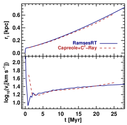
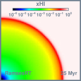
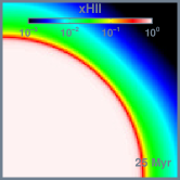
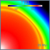
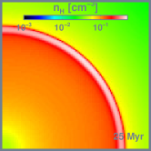
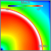
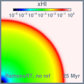
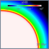
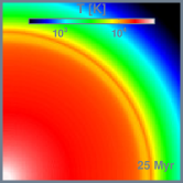
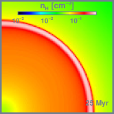
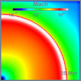
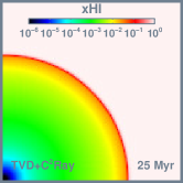
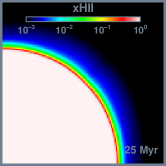
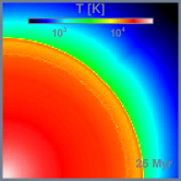
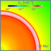
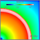
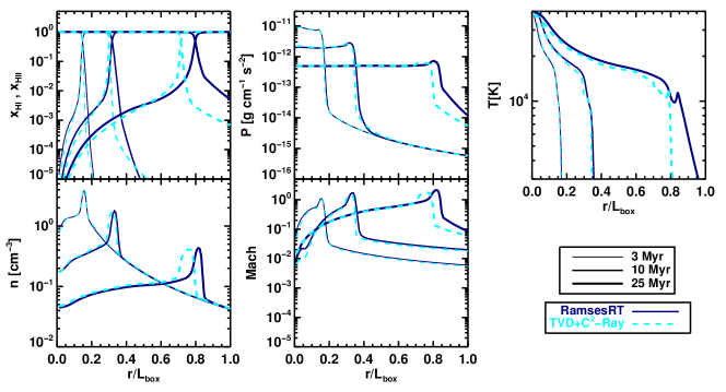
The Strömgren radius for the core density, given by Eq. 47, is $r_{S}\approx 70$ pc, which lies within the flat core. Thus, the I-front makes an initial transition from R-type to D-type within the core, and then may accelerate back to R-type as it expands into decreasingly dense gas outside the core.

We first compare the evolution of the position and speed of the I-front, which is plotted in Fig. 24 for RAMSES-RT and the Capreole+C²-Ray combination. The I-front moves very quickly (R-type) to $\approx 70$ pc within the first fraction of a Myr, stops for while and then starts to expand again with the flow of the gas. Both the speed and position compare well with C²-Ray. The initial speed in C²-Ray has an apparent lag which is due to under-sampling in the front positions at early times, as noted by Il09. Other code results which are better sampled in Il09 show initial speeds that are virtually identical to the RAMSES-RT plot, especially those of the RH1D code. The final front position in RAMSES-RT is slightly further out than that of C²-Ray, though very similar to at least three of the codes in Il09 (Flash-HC, Licorice and RSPH). It also appears that the C²-Ray front is starting to accelerate slightly at the end, whereas the RAMSES-RT front is about to approach constant speed; RAMSES-RT also agrees with most other Il09 codes on this point.

Fig. 25 shows the overall structure of ionization and the gas at $25$ Myr, here with a comparison between RAMSES-RT (upper two rows) and TVD+C²-Ray (bottom row). The Capreole+C²-Ray version of this test is sensitive to so-called ’carbuncle’ numberical instabilities (see Sec. 4.2 in Il09), so we compare here to the more stable and symmetric combination of C²-Ray coupled to the Eulerian TVD solver of Trac & Pen (2004) (used only in this test). In addition to the default RAMSES-RT run with on-the fly AMR refinement, we show here in the middle row results from an identical RAMSES-RT run with the base resolution set to $128^{3}$ cells and AMR refinement turned off. There are slight spherical asymmetries appearing in the top row maps, in particular the $x_{\rm{H\scriptscriptstyle II}}$, $T$ and Mach maps, and the middle row maps are presented here to show that (the first) two of these are purely artifacts of on-the-fly AMR refinement. The slightly square shape of the inner region in the Mach map however does not seem to be due to refinement and is likely rather a grid artifact which is amplified by the radially decreasing density. It should also be noted that the other plots produced for this test (I-front, Fig. 24 and radial profiles, Fig. 26) are absolutely identical regardless of whether on-the-fly refinement is used or the full resolution applied everywhere, suggesting that AMR refinement produces very robust results. The difference in runtime between the AMR and non-AMR runs is actually not much: the AMR run completes in about $2/3$ of the $\sim 640$ cpu hours taken for the non-AMR run. This lack of speedup is due to a combination of a large portion of the grid being refined ($\sim 60\%$ by volume when most), a shallow refinement hierarchy (one level of refinement) and overhead in refinement-related computations.

As usual the I-front is considerably wider in RAMSES-RT than in the C²-Ray results, though we don’t find the same discrepancy as in the previous test between the photoheating intensity close to the source (also, there is no such discrepancy here between C²-Ray and the other codes in Il09). The two maps furthest to the right, of density and Mach number, show the expanding shell of dense gas due to photoheating. Here the shell appears considerably thinner in RAMSES-RT than in TVD+C²-Ray, and indeed TVD+C²-Ray appears to have the thickest density shell of any of the codes in Il09 (Capreole+C²-Ray included, but here there are also severe asymmetries). The RAMSES-RT maps compare well with the C²-Ray ones, and to most of the maps in Il09, and don’t show any I-front instabilities that seem to have a tendency to come up in this test (and Il09 do show that these are numerical and not physical instabilities).

Fig. 26 shows a comparison between RAMSES-RT and TVD+C²-Ray for radially averaged profiles at $3$, $10$ and $25$ Myr of the ionization state, pressure, temperature, density and Mach number. The comparison is generally very good. The I-front (and corresponding density shock) lag a little behind in C²-Ray, but it actually lags a little behind all but one code in this test in Il09, and RAMSES-RT is spot-on compared with those others in every respect.

All in all, RAMSES-RT thus performs well on this test, and no problems appear that are worth mentioning.

6.8 Il09 test 7:   Photo-evaporation of a dense clump

The setup of this test is identical to test 3 in Il06, where UV radiation is cast on a gas cloud, creating a shadow behind it and a slowly-moving I-front inside it. Here however, since the hydrodynamics are turned on, photo-heating causes the cloud to expand outwards and simultaneously contract at the center. We recap the setup:

The box is $L_{\rm{box}}=6.6$ kpc in width. A spherical cloud of gas with radius $r_{\rm{cloud}}=0.8$ kpc is placed at $(x_{c},y_{c},z_{c})=(5,3.3,3.3)$ kpc from the box corner. The density and temperature are $n_{\rm{H}}^{\rm{out}}=2\times 10^{-4}\,{\rm{cm}}^{-3}$ and $T^{\rm{out}}=8000$ K outside the cloud and $n_{\rm{H}}^{\rm{cloud}}=200\,n_{\rm{H}}^{\rm{out}}=4\times 10^{-2}\,{\rm{cm}}^{-3}$ and $T^{\rm{cloud}}=40$ K inside it. From the $x=0$ boundary a constant ionizing flux of $F=10^{6}\;{\rm{photons}}\;{\rm{s}}^{-1}\,{\rm{cm}}^{-2}$ is emitted towards the cloud. The simulation time is $50$ Myr, considerably longer than the $15$ Myr in the corresponding pure RT test. The base resolution is $64^{3}$ cells, but on-the-fly refinement on $n_{\rm{H}}$, $x_{\rm{H\scriptscriptstyle I}}$ and $x_{\rm{H\scriptscriptstyle II}}$ gradients ensures the prescribed effective resolution of $128^{3}$ cells at ionization and shock fronts. In order to best capture the formation of a shadow behind the cloud, we focus on a RAMSES-RT run with the HLL solver, but we also show some results with the usual GLF solver.

(a)

(b)

(c)

(d)

(e)

(f)

(g)

(h)

(i)

(j)

(k)

(l)

(m)

(n)

(o)

(p)

(q)

(r)

(s)

(t)

(u)

(v)

(w)

(x)

(y)

(z)

(aa)

(ab)

(ac)

(ad)

Figure 27: Il09 test 7. Maps showing slices at $z=0.5\ L_{\rm{box}}$ of various quantities at 10 Myrs (top panel) and 50 Myrs (lower panel). In each panel, the top row shows the RAMSES-RT+HLL results, the middle row shows RAMSES-RT+GLF and the bottom row shows the Capreole+C²-Ray results.

(a)

(b)

Figure 28: Il09 test 7. (a) Time evolution of the position (top) and speed (bottom) of the ionization front along the x-axis of symmetry through the center of the box. (b) Histograms of the gas temperature (upper panel) and flow Mach number (lower panel) at 10 and 50 Myr for RAMSES-RT and Capreole+C²-Ray.

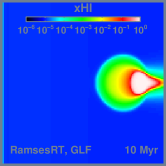
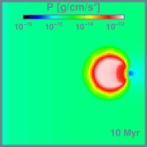
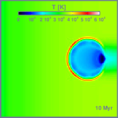
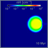
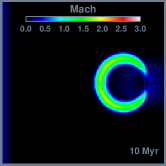
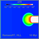
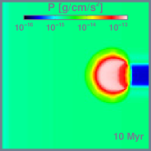
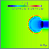
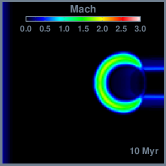
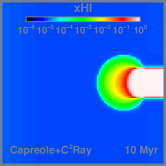
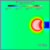
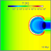
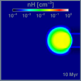
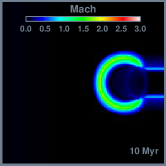
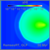
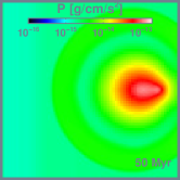
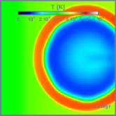
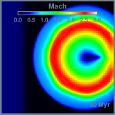
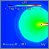
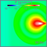
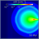
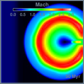
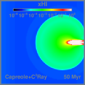
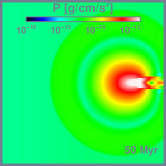
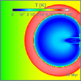
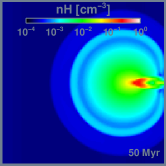
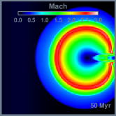
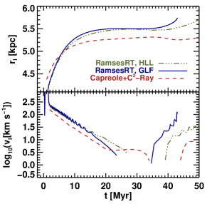
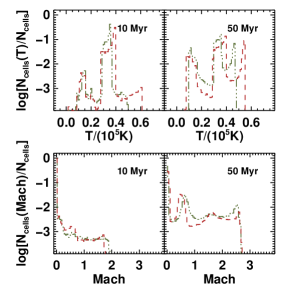
Fig. 27 shows slices in the $xy$-plane through the middle of the box of various quantities at $10$ and $50$ Myr, for the RAMSES-RT result and C²-Ray for comparison. As in the corresponding pure RT test, it can be seen from the $x_{\rm{H\scriptscriptstyle I}}$ maps that the shadow behind the cloud is less conserved with RAMSES-RT than with C²-Ray, though the HLL solver does a much better job though than GLF. However, the diffusion of photons doesn’t have a large impact on the resulting dynamics, or even the propagation of the I-front along the axis of symmetry. The shadow becomes thinner towards the end of the run with all codes in Il09, though it is thinner than most in RAMSES-RT+HLL, and it pretty much disappears in RAMSES-RT+GLF. The shadow thickness in RAMSES-RT+HLL is still comparable at $50$ Myrs to the results of RSPH, Zeus-MP and Licorice in Il09. The pressure maps of RAMSES-RT+HLL, C²-Ray and other codes in Il09 are very similar both at $10$ and $50$ Myrs, though C²-Ray, and also to some extent Flash-HC and Licorice have a fork-like shape inside what remains of the shadow at $50$ Myr. The other codes have the same shape as RAMSES-RT+HLL in this region. The temperature maps are similar as well, though the backwards-expanding cloud shell seems to be slightly less shock-heated in RAMSES-RT than most other codes. The shell expands in a very similar way for the two codes, as can be seen in the density and Mach slices. The expansion goes a bit further, though, in RAMSES-RT. Also, the expanding cloud seems to develop a slightly hexagonal shape in RAMSES-RT, an effect which is not apparent in any of the codes in this test in Il09 (though there is a hint of it in the Flash-HC result). It can only be speculated that this is a grid artifact. To be sure it doesn’t have to do with the on-the-fly refinement we ran an identical experiment with a base resolution of $128^{3}$ cells and no refinement in RAMSES-RT+HLL. The RAMSES-RT+HLL maps and plots presented here are virtually identical to this non-refinement run, except of course for graininess in the slice maps. None of these discussed effects (hexagons and a slightly over-extended I-front compared to other codes) are thus due to on-the-fly refinement. As in the previous test, the speed-wise gain in using AMR is not a lot: the AMR run completes in about half of the $\sim 64$ cpu hours taken for the non-AMR run. Again the relatively modest speedup is due to a combination of a large portion of the grid being refined ($\sim 30\%$ by volume when most), a shallow refinement hierarchy, and refinement-related overhead. With deeper refinement hierarchies in cosmological simulations, the speedup can be much greater, but a quantitative demonstration is beyond the scope of this paper.

Figure 29: Il09 test 7. Profiles along the x-axis of symmetry through the center of the box, at 1, 10 and 50 Myr for the RAMSES-RT and Capreole+C²-Ray results. Clockwise from top left: ionization fractions, pressure, temperature, Mach number, atom number density.

Next we turn our attention to the evolution of the position and speed of the I-front along the x-axis of symmetry through the box. This is presented for the RAMSES-RT (HLL and GLF) and C²-Ray runs in Fig. 28a. The I-front propagation is considerably different between RAMSES-RT and C²-Ray, but actually C²-Ray considerably stands out here from other codes in Il09. For the first 7 Myrs or so, the RAMSES-RT front lags behind that of C²-Ray and in fact all the codes in Il09. This is due to the reduced speed of light: before hitting the cloud, the photons have to travel from the left edge of the box through a very diffuse medium – so diffuse that here the I-front speed apparently is approaching the speed of light, or is at least considerably faster than the one-one-hundredth of the light speed which is used in the RAMSES-RT run. However, once the I-front in the RAMSES-RT run has caught up, the reduced light speed should have a negligible effect on the results. After roughly 7 Myr, the RAMSES-RT I-front overtakes C²-Ray front, and stays ahead of it for the remainder of the run. This however is also the case for most of the codes in Il09; their I-front is ahead of the C²-Ray front, and four out of six codes end up with the I-front at $\sim 5.6$ kpc. The RAMSES-RT+HLL front ends up at $\sim 5.7$ kpc, so slightly ahead of what is typically found in Il09. Using the GLF solver instead of HLL has the effect that the I-front disappears soon after $40$ Myrs, which is due to diffusive photons eating into the shadow from it’s edges, but up to that point the I-front evolution is much the same. RAMSES-RT also reproduces the retreat of the I-front between roughly 30 and 40 Myrs, which is seen in all runs in Il09. This momentary negative speed is due to the expansion of the cloud and the D-type movement of the I-front with the gas.

Fig. 28b shows histograms of the gas temperature and Mach number at $10$ and $50$ Myr in the RAMSES-RT+HLL and C²-Ray runs. The shapes of the histograms are very similar between the two codes (and are also very similar to RAMSES-RT+GLF, which is not shown).

Finally, Fig. 29 shows a comparison between RAMSES-RT and C²-Ray of profiles along the x-axis of symmetry of the various quantities at $1$, $10$ and $50$ Myrs. The profiles compare badly at $1$ Myr, but as already discussed this is simply due to the I-front having not caught up at this early time when using the reduced speed of light. At later times the profiles generally compare well, though we see these effects which have already been discussed, of a further expanding density-front out of the original cloud, and a further progressed I-front. The RAMSES-RT profile plots show a staircase effect which is most obvious in the $50$ Myrs plot at the radial interval $0.45\la r/L_{\rm{box}}\la 0.75$: this is simply due to the grid being unrefined at this x-interval along the axis of symmetry, i.e. at the effective base resolution of $64^{3}$ cells per box width. The run with the full resolution and no AMR refinement shows no staircases, but otherwise the results are identical to those shown here.

We have made an alternative run with RAMSES-RT+HLL with the speed of light fraction set to $f_{c}=1/10$ rather than the default $1/100$, and here the initial evolution of the I-front position and radial profiles at $1$ Myr are almost identical to those of C²-Ray. At later times the results are very much in line with those where $f_{c}=1/100$, except the I-front position is slightly more advanced at $50$ Myr, or at $5.78$ kpc rather than at $5.71$ kpc.

In summary, RAMSES-RT performs well on this test with no apparent problems. The reduced light speed ($f_{c}=1/100$) has very little effect on the results and on-the-fly refinement gives results which are identical to the fully refined simulation with a homogeneous $128^{3}$ cells grid. Even using the diffusive GLF solver retains much of the results (I-front development, cloud expansion), except that the I-front disappears a bit prematurely.

6.9 RT test conclusions

RAMSES-RT performs very well on all the tests from Il06 and Il09, with no discrepancies to speak of from expected results or those from other codes.

The most notable discrepancies clearly result from the reduced speed of light approximation, which leads to I-fronts that are initially too slow compared to full speed of light runs – or infinite speed, as is the case for many of the codes compared against from the RT comparison project. In test 4, the high-z cosmological field, we actually demostrated the reverse, where the codes we compared to had considerably premature I-fronts as a consequence of their infinite light speed approximations. Our shadows are considerably shorter lived with the GLF intercell flux function than those of the other codes (most of which use ray-tracing schemes). This can be fixed for problems involving shadows and idealized geometries by using the HLL flux function instead, but as we showed in §3.2 the sacrifice is that isotropic sources become anisotropic. Many codes in the RT comparison project show various instabilities and asymmetries in ionization fronts; no such features are manifested in the RAMSES-RT results.

7 Discussion

In this paper, we have presented a new implementation of radiation hydrodynamics in the RAMSES code. It is based on a moment representation of the radiation field, where we have used the M1 closure relation to define a purely local variable Eddington tensor. Because the resulting system is a set of hyperbolic conservation laws, we have exploited the Godunov methodology to design a time-explicit, strictly photon conserving radiation transport scheme. The resulting algorithm is first order accurate in space and time, and uses various Riemann solvers (GLF and HLL) to compute radiation fluxes. The main novelty compared to our previous implementation (AT08) is the coupling between gas and radiation, resulting in a fully consistent radiation hydrodynamics solver, and the introduction of adaptive mesh techniques in the radiation transport step, making use of both the AMR and parallel computing capabilities of RAMSES. Overall, the code was quite easy to implement, owing to the explicit nature of the time integration scheme. The price to pay is the need to resolve the propagation of hyperbolic waves traveling at or close to the speed of light. Among many different options available to overcome this constraint, we have chosen to use the “reduced speed of light” approximation. This approximation is valid when the propagation speed of I-fronts is still slower than the (reduced) light speed. We have developed a recipe to assess the validity of this approximation, based on the light-crossing time of Strömgren spheres. We have verified that this framework indeed allows us to estimate in advance the speed-of-light reduction factor reliably. We have shown, for example, that in cosmological problems, such as cosmic reionization, using the correct value for the speed of light is crucial, and using either a reduced or an infinite speed of light (like in some ray-tracing codes) might result in large inaccuracies.

This new algorithm has already been used in galaxy formation studies, exploiting the coupling between radiation and hydrodynamics offered by RAMSES-RT. In Rosdahl & Blaizot (2012), we studied the impact of ionizing radiation in determining the thermal state of cold filaments streaming into high redshift galaxies, allowing us to make accurate observational predictions and demonstrating a possible link between cold streams and Lyman-alpha blobs. More recently, we have also explored the role of ionizing radiation in the overall efficiency of stellar feedback (Geen et al. 2013, Powell et al. 2013, both in preparation). Beyond ionizing radiation, possible extensions of RAMSES-RT are the inclusion of photo-dissociating radiation and the thermochemistry of molecules, as well as the effect of dust as an additional source of opacity and thermal regulation inside star forming galaxies. This would require introducing additional photon groups (such as a far UV and IR photons) and the associated microphysics, but the overall methodology would remain very similar.

In order to improve the current algorithm, we have many possibilities ahead of us. One obvious development is to develop a second-order sequel of our current first order Godunov solver. Second-order Godunov schemes, both in time and space, are used routinely in hydrodynamics codes (such as the MUSCL scheme in RAMSES). This might reduce significantly the rather large diffusivity of our current implementation. However, since photo-ionization and photo-dissociation problems are governed to a large extent by the thermo-chemistry, it is not clear how much the accuracy of the results would depend on the advection scheme. A second route we would like to explore in the future is the optional introduction of radiation sub-cycles during each adaptive hydro step. This is quite challenging since it would in principle require decoupling in time of the various AMR levels, resulting in the loss of strict photon conservation. In some cases, however, it is advantageous to sacrifice the exact number conservation of photons in favour of modelling the correct speed of light with many radiation sub-cycles. In any case, this would offer us a new tool with greater flexibility. Along the same lines, because of the fundamentally different propagation properties of I-fronts in the IGM on one hand and deep inside galaxies on the other, we could couple RAMSES-RT to ATON: use ATON to transport radiation on the coarse grid with GPUs at the full speed of light, and use RAMSES-RT on the fine AMR levels at a reduced light speed. This would require us to define two photon group populations that mirror each other: a large scale, low density photon population that propagates at the correct speed of light and makes use of GPU acceleration (if available), and a small scale, high density photon population that makes use of the “reduced speed of light” approximation. Coupling properly the two photon group populations will of course be quite challenging and at the heart of this new avenue of research. A last development we have in mind is the introduction of radiation pressure as a new channel of coupling radiation with hydrodynamics. This is highly relevant for studies focusing on radiation pressure on dust, from both young star clusters and supermassive black holes.

Appendix A RamsesRT non-equilibrium thermochemistry

We describe here in detail the non-equilibrium thermochemistry we have implemented for RAMSES-RT to accommodate for the interactions between photons and gas. A thermochemistry step in RAMSES-RT considers a single cell of gas at a time with a given state ${\mathcal{U}}=(\rho,\rho{\bf{u}},E,\rho x_{\rm{H\scriptscriptstyle II}},\rho x_{\rm{He\scriptscriptstyle II}},\rho x_{\rm{He\scriptscriptstyle III}},N_{i},{\bf{F}}_{i})$ (respectively, mass density, momentum density, energy density, hydrogen and helium ion abundances, photon densities and fluxes) and evolves numerically over a time-step $\Delta t$ the thermochemical state

$${\mathcal{U}}_{T}=\left(\begin{matrix}{\varepsilon},\ x_{\rm{H\scriptscriptstyle II}},\ x_{\rm{He\scriptscriptstyle II}},\ x_{\rm{He\scriptscriptstyle III}},\ N_{1},\ ..\ N_{M},\ F_{1},\ ..\ F_{M}\end{matrix}\right)$$ (49)

(where ${\varepsilon}=E-1/2\rho{\bf{u}}^{2}$ is the thermal energy density), i.e. solves the set of $4+2M$ coupled equations

$$\frac{\partial{\mathcal{U}}_{T}}{\partial t}={\mathcal{S}},$$ (50)

where ${\mathcal{S}}\equiv\dot{{\mathcal{U}}_{T}}$.

Due to the stiffness of the thermochemistry equations, it is feasible to solve them implicitly, i.e. using ${\mathcal{S}}({\mathcal{U}}_{T}^{t+\Delta t})$ on the right hand side (RHS), which guarantees stability and convergence of the solver. However a fully implicit solver is complicated in implementation, computationally expensive and not easily adaptable to changes, e.g. a varying number of photon groups or additional ion/chemical abundances. Instead we take an approach inspired by Anninos et al. (1997). The idea is to solve one equation at a time in a specific order, and on the RHS use forward-in-time (FW) values, i.e. evaluated at $t+\Delta t$, wherever available, but otherwise backwards-in-time (BW) values, evaluated at $t$. So for the first variable we choose to advance in time, there are no FW variables available. For the next one, we can use the FW state of the first variable, and so on. In that sense the method can be thought of as being partially implicit.

The cell-thermochemistry is called once every RT time-step of length $\Delta t_{RT}$, but in each cell it is split into local sub-steps of length $\Delta t$ that adhere to the $10\%$ rule,

$$\rm{max}\left(\left|\frac{\Delta{\mathcal{U}}_{T}}{{\mathcal{U}}_{T}}\right|\right)\leq 0.1,$$ (51)

where $\Delta{\mathcal{U}}_{T}$ is the change in ${\mathcal{U}}_{T}$ during the sub-step. The RT step thus contains a loop for each cell, which calls the $\tt{thermo\_step({\mathcal{U}}_{T},\Delta t)}$ routine once or more often: first with $\Delta t=\Delta t_{RT}$, then possibly again a number of times to fill in $\Delta t_{RT}$ if the first guess at $\Delta t$ proves too long to meet the condition set by (51).

The $\tt{thermo\_step({\mathcal{U}}_{T},\Delta t)}$ routine performs the following tasks:

1. $N$ and $F$ update

2. $E$ update

3. $x_{\rm{H\scriptscriptstyle I}}$ update

4. $x_{\rm{He\scriptscriptstyle II}}$ and $x_{\rm{He\scriptscriptstyle III}}$ update

5. Check if we are safe to use a bigger time-step

Tasks 2 to 4 are in the same order as in Anninos et al. (1997), but they don’t include radiative transfer in their code, so there is no photon update. The argument we have for putting it first rather than anywhere else is that the photon densities appear to be the most dynamic variables and so are also most likely to break the time-step condition (51). This we want to catch early on in the thermochemistry step so we avoid doing calculations of tasks 2 to 5 that turn out to be useless because of the too-long time-step.

We now describe the individual tasks. Temperature dependent interaction rates frequently appear in the tasks - their expressions are given in Appendix E. The temperature can at any point be extracted from the energy density and ionization state of the gas via

$$T={\varepsilon}\ \frac{(\gamma-1)m_{H}}{\rho k_{\rm{B}}}\ \mu,$$ (52)

where $\gamma$ is the ratio of specific heats (usually given the value of $5/3$ in RAMSES, corresponding to monatomic gas), $m_{H}$ the proton mass, $k_{\rm{B}}$ the Boltzmann constant and $\mu$ is the average mass per particle in the gas, in units of $m_{H}$.

1 Photon density and flux update

The photon number densities and fluxes, $N_{i}$ and $F_{i}$, are updated one photon group $i$ at a time. For the photon density the equations to solve are

$$\frac{\partial N_{i}}{{\partial t}}={\dot{N}}_{i}+C_{i}-N_{i}\,D_{i},$$ (53)

where ${\dot{N}}_{i}$ represents the time derivative of $N_{i}$ given by the RT transport solver (which is nonzero only if the smoothed RT option is used), $C_{i}$ represents photon-creating re-combinations, and $D_{i}$ represents photon-destroying absorptions. The creation term is non-existent if the OTSA is used (emitted photons are assumed to be immediately reabsorbed), but is otherwise given by

$$C_{i}=\sum_{j}^{\rm{H\textsc{ii}},\rm{He\textsc{ii}},\rm{He\textsc{iii}}}b^{rec}_{ji}\ (\alpha^{\rm{A}}_{j}-\alpha^{\rm{B}}_{j})\ n_{j}\ n_{e},$$ (54)

where the $b^{rec}_{ji}$ factor is a boolean (1/0) that states which photon group $j$-species recombinations emit into and $\alpha^{\rm{A}}_{j}$ and $\alpha^{\rm{B}}_{j}$ are the temperature dependent case A and B recombination rates for the recombining species. The photon destruction factor is given by

$$D_{i}=\sum_{j}^{{\rm{H\textsc{i}}},{\rm{He\textsc{i}}},\rm{He\textsc{ii}}}{c_{r}}\ {\sigma}^{\rm{N}}_{ij}\ n_{j},$$ (55)

where ${c_{r}}$ is the (reduced) light speed and ${\sigma}^{\rm{N}}_{ij}$ is the cross-section between species $j$ and photons in group $i$.

Photon emission from recombination is assumed to be spherically symmetric, i.e. to go in all directions. It is therefore purely a diffusive term, and the photon flux equation only includes the photo-absorbtions:

$$\frac{\partial F_{i}}{{\partial t}}={\dot{F}}_{i}-F_{i}\,D_{i},$$ (56)

where ${\dot{F}}_{i}$ is the time derivative used only in smoothed RT and the destruction factor remains as in (55).

Equations (53) and (56) are solved numerically using a partly semi-implicit Euler (SIE) formulation, in the sense that they are semi-implicit in the photon density and flux but otherwise explicit (in temperature and the ion abundances). A tiny bit of algebra gives:

$$N_{i}^{\,t+\Delta t} =\frac{N_{i}^{\,t}+\Delta t({\dot{N}}_{i}+C_{i})}{1+\Delta tD_{i}},$$ (57)

$$F_{i}^{\,t+\Delta t} =\frac{F_{i}^{\,t}+\Delta t{\dot{F}}_{i}}{1+\Delta tD_{i}},$$ (58)

where all the variables at the RHS are evaluated at the beginning of the time-step, i.e. at $t$.

For each photon group update, the $10\%$ rule is checked: if

$$\frac{\left|N^{t+\Delta t}_{i}-N^{t}_{i}\right|}{N_{i}^{t}}>0.1,$$ (59)

the $\tt{cool\_step}$ routine returns with an un-updated state but instead a recommendation for a new time-step length $\Delta t_{new}=0.5\ \Delta t$, so the routine can be called again with a better chance of completing.

2 Thermal update

Due to the dependency of $\mu$ on the ionization fractions it is easiest to evolve the quantity

$$T_{\mu}\equiv\frac{T}{\mu},$$ (60)

where $\mu$ can be extracted via

$$\mu=\left[\,X(1+x_{\rm{H\scriptscriptstyle II}})+Y/4(1+x_{\rm{He\scriptscriptstyle II}}+2x_{\rm{He\scriptscriptstyle III}})\,\right]^{-1},$$ (61)

with $X$ and $Y=1-X$ the hydrogen and helium mass fractions, respectively. Here we ignore the metal contribution to $\mu$, which in most astrophysical contexts is negligible.

The temperature is updated by solving

$$\frac{\partial T_{\mu}}{\partial t}=\frac{(\gamma-1)m_{\rm{H}}}{\rho k_{\rm{B}}}\ {\Lambda},$$ (62)

where ${\Lambda}\equiv\dot{{\varepsilon}}={\mathcal{H}}+{\mathcal{L}}$, ${\mathcal{H}}$ is the photoheating rate and ${\mathcal{L}}$ the cooling rate. These rates are calculated as follows:

The photoheating rate ${\mathcal{H}}$ is a sum of the heating contributions from all photoionization events:

$$\mathcal{H}=\sum_{j}^{\rm{{\rm{H\textsc{i}}}{},{\rm{He\textsc{i}}}{},\rm{He\textsc{ii}}{}}}n_{j}\int_{0}^{\infty}\sigma_{j}(\nu)F(\nu)\left[h\nu-\epsilon_{j}\right]d\nu,$$ (63)

where $\nu$ is photon frequency, $F(\nu)$ local photon flux and $\epsilon_{j}$ photoionization energies. With the discretization into $M$ photon groups, (63) becomes

$$\mathcal{H}=\sum_{j}^{\rm{{\rm{H\textsc{i}}},{\rm{He\textsc{i}}},\rm{He\textsc{ii}}}}n_{j}\sum_{i=1}^{M}{c_{r}}N_{i}\left(\bar{\epsilon}_{i}{\sigma}^{\rm{E}}_{ij}-\epsilon_{j}{\sigma}^{\rm{N}}_{ij}\right)$$ (64)

where $\bar{\epsilon}_{i}$, ${\sigma}^{\rm{N}}_{ij}$, ${\sigma}^{\rm{E}}_{ij}$ and are the photon average energies, average cross sections and energy weighted cross sections, respectively, for ionization events between group $i$ and species $j$ (see Eqs. 9-11).

The primordial cooling rate ${\mathcal{L}}$ is given by

$${\mathcal{L}} =\left[\zeta_{{\rm{H\textsc{i}}}}(T)+\psi_{{\rm{H\textsc{i}}}}(T)\right]\ n_{\rm{e}}\ n_{\rm{H\scriptscriptstyle I}}$$ (65)

$$+\zeta_{{\rm{He\textsc{i}}}}(T)\ n_{\rm{e}}\ n_{\rm{He\scriptscriptstyle I}}$$

$$+\left[\zeta_{\rm{He\textsc{ii}}}(T)+\psi_{\rm{He\textsc{ii}}}(T)+\eta^{\rm{A}}_{\rm{He\textsc{ii}}}(T)+\omega_{\rm{He\textsc{ii}}}(T)\right]n_{\rm{e}}n_{\rm{He\scriptscriptstyle II}}$$

$$+\eta^{\rm{A}}_{\rm{H\textsc{ii}}}(T)\ n_{\rm{e}}\ n_{\rm{H\scriptscriptstyle II}}$$

$$+\eta^{\rm{A}}_{\rm{He\textsc{iii}}}(T)\ n_{\rm{e}}\ n_{\rm{He\scriptscriptstyle III}}$$

$$+\theta(T)\ n_{\rm{e}}\left(n_{\rm{H\scriptscriptstyle II}}+n_{\rm{He\scriptscriptstyle II}}+4n_{\rm{He\scriptscriptstyle III}}\right)$$

$$+\varpi(T)\ n_{\rm{e}},$$

where the various cooling processes are collisional ionizations $\zeta$, collisional excitations $\psi$, recombinations $\eta$, dielectronic recombinations $\omega$, bremsstrahlung $\theta$ and Compton cooling $\varpi$, all analytic (fitted) functions of temperature taken from various sources. The complete expressions are listed (with references) in Appendix E. If the OTSA is used, the $\eta^{\rm{A}}$ coefficients are replaced with $\eta^{\rm{B}}$.

The temperature update (62) is solved numerically using semi-implicit formulation in $T_{\mu}$, using FW values of photon densities and BW values of H and He species abundances. The temperature is updated to

$$T_{\mu}^{t+\Delta t}=T_{\mu}^{t}+\frac{{\Lambda}K\Delta t}{1-{\Lambda^{\prime}}K\Delta t},$$ (66)

where $K\equiv\frac{(\gamma-1)m_{\rm{H}}}{\rho k_{\rm{B}}}$. The temperature-derivative, ${\Lambda^{\prime}}\equiv\frac{\partial{\mathcal{L}}}{\partial T_{\mu}}$, is found by algebraically differentiating each of the primordial cooling rate expressions in the case of ${\mathcal{L}}$ (and using $\frac{\partial{\mathcal{L}}}{\partial T_{\mu}}=\mu\frac{\partial{\mathcal{L}}}{\partial T}$). The temperature derivative of the heating rate is zero.

With $T_{\mu}^{t+\Delta t}$ in hand, the time-stepping condition is checked, i.e if

$$\frac{\left|T_{\mu}^{t+\Delta t}-T_{\mu}^{t}\right|}{T_{\mu}^{t}}>0.1,$$ (67)

$\tt{cool\_step}$ is re-started with half the time-step length. In tests we’ve found that the usual time-step constraint given here is not enough to ensure stability, as the temperature in some cases oscillates, even in a divergent way. ${\Lambda}$ and ${\Lambda^{\prime}}$ are both evaluated backwards in time, i.e. at $t$, and the large difference that can exist in these values from $t$ to $t+\Delta t$ appears to cause these instabilities. To fix that we include also a first-order time-step constraint on the temperature, i.e. if

$$\frac{\left|K{\Lambda}\Delta t\right|}{T_{\mu}^{t}}>0.1,$$ (68)

the time-step length is halved. With this fix, we have not seen further temperature oscillations, but there is no guarantee that numerical instabilities are eliminated.

3 Hydrogen ionized fraction update

The Hii abundance is affected by collisional ionizations, photoionizations, and recombinations, i.e.

$$\frac{{\partial}n_{\rm{H\scriptscriptstyle II}}}{{\partial t}}=n_{\rm{H\scriptscriptstyle I}}\left(\beta_{{\rm{H\textsc{i}}}}n_{\rm{e}}+\sum_{i=1}^{M}{\sigma}^{\rm{N}}_{i{\rm{H\textsc{i}}}}{c_{r}}N_{i}\right)-n_{\rm{H\scriptscriptstyle II}}\alpha^{\rm{A}}_{\rm{H\scriptscriptstyle II}}n_{\rm{e}},$$ (69)

where $\beta_{{\rm{H\textsc{i}}}}(T)$ is the rate of collisional ionizations by electrons and $\alpha^{\rm{A}}_{\rm{H\scriptscriptstyle II}}(T)$ the case A hydrogen recombination rate, which is replaced here by $\alpha^{\rm{B}}_{\rm{H\scriptscriptstyle II}}$ if the OTSA is used. In terms of ionization fraction, (69) becomes

$$\frac{{\partial}x_{\rm{H\scriptscriptstyle II}}}{{\partial t}} =(1-x_{\rm{H\scriptscriptstyle II}})\left[\beta_{{\rm{H\textsc{i}}}}n_{\rm{e}}+\sum_{i=1}^{M}{\sigma}^{\rm{N}}_{i{\rm{H\textsc{i}}}}{c_{r}}N_{i}\right]-x_{\rm{H\scriptscriptstyle II}}\alpha^{\rm{A}}_{\rm{H\scriptscriptstyle II}}n_{\rm{e}}$$

$$=(1-x_{\rm{H\scriptscriptstyle II}})\ C-x_{\rm{H\scriptscriptstyle II}}\ D$$

$$=C-x_{\rm{H\scriptscriptstyle II}}\ (C+D),$$ (70)

where we have in the second line separated the rates into Hii creation $C$ and destruction $D$, and in the third line collected multiples of $x_{\rm{H\scriptscriptstyle II}}$.

To prevent stiffness-induced instabilities, we have gone for an approach which is semi-implicit in $x_{\rm{H\scriptscriptstyle II}}$:

$$x_{\rm{H\scriptscriptstyle II}}^{t+\Delta t}=x_{\rm{H\scriptscriptstyle II}}^{t}+\Delta t\frac{C-x_{\rm{H\scriptscriptstyle II}}^{t}(C+D)}{1-J\Delta t},$$ (71)

where

$$J \equiv\frac{{\partial}\dot{x}_{\rm{H\textsc{ii}}}}{{\partial}x_{\rm{H\scriptscriptstyle II}}}$$

$$=\frac{{\partial}C}{{\partial}x_{\rm{H\scriptscriptstyle II}}}-(C+D)-x_{\rm{H\scriptscriptstyle II}}\left(\frac{{\partial}C}{{\partial}x_{\rm{H\scriptscriptstyle II}}}+\frac{{\partial}D}{{\partial}x_{\rm{H\scriptscriptstyle II}}}\right),$$ (72)

and the creation and destruction derivatives are given by

$$\frac{{\partial}C}{{\partial}x_{\rm{H\scriptscriptstyle II}}} =n_{\rm{H}}\beta_{{\rm{H\textsc{i}}}}-n_{\rm{e}}T_{\mu}\mu^{2}X\frac{{\partial}\beta_{{\rm{H\textsc{i}}}}}{{\partial}T}$$ (73)

$$\frac{{\partial}D}{{\partial}x_{\rm{H\scriptscriptstyle II}}} =n_{\rm{H}}\alpha^{\rm{A}}_{\rm{H\scriptscriptstyle II}}-n_{\rm{e}}T_{\mu}\mu^{2}X\frac{{\partial}\alpha^{\rm{A}}_{\rm{H\scriptscriptstyle II}}}{{\partial}T}.$$ (74)

We end with the usual check if the $10\%$ rule is broken, i.e. if

$$\frac{\left|x_{\rm{H\scriptscriptstyle II}}^{t+\Delta t}-x_{\rm{H\scriptscriptstyle II}}^{t}\right|}{x_{\rm{H\scriptscriptstyle II}}^{t}}>0.1,$$ (75)

$\tt{cool\_step}$ is restarted with half the time-step length. Like with the temperature a first-order check is also made, i.e.

$$\frac{\left|C-x_{\rm{H\scriptscriptstyle II}}^{t}(C+D)\right|}{x_{\rm{H\scriptscriptstyle II}}^{t}}\Delta t>0.1.$$ (76)

4 Helium ionized fractions update

Though the Hei fraction is not a cell variable (it can be obtained via $x_{\rm{He\scriptscriptstyle I}}=1-x_{\rm{He\scriptscriptstyle II}}-x_{\rm{He\scriptscriptstyle III}}$), it is evolved in order to make a consistency check at the end of the helium updates. Before each of the helium fraction updates, we recalculate $n_{\rm{e}}$ and $\mu$ to reflect the new FW abundances.

The Hei fraction is set by

$$\frac{{\partial}x_{\rm{He\scriptscriptstyle I}}}{{\partial t}} =x_{\rm{He\scriptscriptstyle II}}\alpha^{\rm{A}}_{\rm{He\textsc{ii}}}n_{\rm{e}}-x_{\rm{He\scriptscriptstyle I}}\left(\beta_{{\rm{He\textsc{i}}}}n_{\rm{e}}-\sum_{i=1}^{M}{\sigma}^{\rm{N}}_{i{\rm{He\textsc{i}}}}{c_{r}}N_{i}\right)$$

$$=\ C\ -\ x_{\rm{He\scriptscriptstyle I}}\ D,$$ (77)

i.e. Heii recombinations and collisional- and photo-ionizations of Hei. As usual $\alpha^{\rm{A}}$ is replaced by $\alpha^{\rm{B}}$ in the case of the OTSA. In the second line of (A) we’ve separated the RHS into Hei creation $C$ and destruction $D$.

Here we follow Anninos et al. (1997) and do the Hei update with

$$x_{\rm{He\scriptscriptstyle I}}^{t+\Delta t}=\frac{x_{\rm{He\scriptscriptstyle I}}^{t}+C\Delta t}{1+D\Delta t}.$$ (78)

The update is partly implicit, since it uses updated values of $N_{i}^{t+\Delta t}$, $T_{\mu}^{t+\Delta t}$, and $x_{\rm{H\scriptscriptstyle II}}^{t+\Delta t}$ ($\rightarrow$ $\mu$ and $n_{\rm{e}}$), but un-updated values of $x_{\rm{He\scriptscriptstyle II}}^{t}$ and $x_{\rm{He\scriptscriptstyle III}}^{t}$.

We then evolve the Heii fraction. The differential equation to solve is

$$\frac{{\partial}x_{\rm{He\scriptscriptstyle II}}}{{\partial t}} =x_{\rm{He\scriptscriptstyle I}}\left(\beta_{{\rm{He\textsc{i}}}}n_{\rm{e}}+\sum_{i=1}^{M}{\sigma}^{\rm{N}}_{i{\rm{He\textsc{i}}}}{c_{r}}N_{i}\right)+x_{\rm{He\scriptscriptstyle III}}\alpha^{\rm{A}}_{\rm{He\textsc{iii}}}n_{\rm{e}}$$

$$-x_{\rm{He\scriptscriptstyle II}}\left(\beta_{\rm{He\textsc{ii}}}n_{\rm{e}}+\alpha^{\rm{A}}_{\rm{He\textsc{ii}}}n_{\rm{e}}+\sum_{i=1}^{M}{\sigma}^{\rm{N}}_{i\rm{He\textsc{ii}}}{c_{r}}N_{i}\right)$$

$$=C\ -\ x_{\rm{He\scriptscriptstyle II}}\ D.$$ (79)

The RHS terms are, in order of appearance, Hei collisional ionizations, Heiii recombinations, Hei photoionizations (with an optional homogeneous background in parentheses), Heii collisional ionizations, Heii recombinations and Heii photo-ionizations. In the third line we have grouped the terms into a creation term $C$ and destruction terms $D$.

The discrete update is done with the same formulation as (78), i.e.

$$x_{\rm{He\scriptscriptstyle II}}^{t+\Delta t}=\frac{x_{\rm{He\scriptscriptstyle II}}^{t}+C\Delta t}{1+D\Delta t},$$ (80)

using updated values of $N_{i}^{t+\Delta t}$, $T_{\mu}^{t+\Delta t}$, $x_{\rm{H\scriptscriptstyle II}}^{t+\Delta t}$, and $x_{\rm{He\scriptscriptstyle I}}^{t+\Delta t}$ ($\rightarrow$ $\mu$ and $n_{\rm{e}}$), and the un-updated value only of $x_{\rm{He\scriptscriptstyle III}}^{t}$.

The only variable left is the Heiii fraction. The differential equation is

$$\frac{{\partial}x_{\rm{He\scriptscriptstyle III}}}{{\partial t}} =x_{\rm{He\scriptscriptstyle II}}\left(\beta_{\rm{He\textsc{ii}}}n_{\rm{e}}+\sum_{i=1}^{M}{\sigma}^{\rm{N}}_{i\rm{He\textsc{ii}}}{c_{r}}N_{i}\right)$$

$$-x_{\rm{He\scriptscriptstyle III}}\ \alpha^{\rm{A}}_{\rm{He\textsc{iii}}}n_{\rm{e}}$$

$$=\ C\ -\ x_{\rm{He\scriptscriptstyle III}}\ D.$$ (81)

In the third line we have as usual grouped the terms into creation and destruction.

Again the update follows the same formulation,

$$x_{\rm{He\scriptscriptstyle III}}^{t+\Delta t}=\frac{x_{\rm{He\scriptscriptstyle III}}^{t}+C\Delta t}{1+D\Delta t},$$ (82)

which is implicit in all variables.

Conservation of helium density is then enforced, i.e. that

$$x_{\rm{He\scriptscriptstyle I}}+x_{\rm{He\scriptscriptstyle II}}+x_{\rm{He\scriptscriptstyle III}}=1,$$ (83)

by lowering the largest of these fractions accordingly (in the case of $x_{\rm{He\scriptscriptstyle I}}$ being the largest there is no update).

The $10\%$ rule is not applied to the helium fractions. Instead, the final $10\%$ check is done on the electron density, which is retrieved from all the ionization fractions with

$$n_{\rm{e}}=x_{\rm{H\scriptscriptstyle II}}n_{\rm{H}}+(x_{\rm{He\scriptscriptstyle II}}+2x_{\rm{He\scriptscriptstyle III}})n_{\rm{He}}.$$ (84)

If

$$\frac{\left|n_{\rm{e}}^{t+\Delta t}-n_{\rm{e}}^{t}\right|}{n_{\rm{e}}^{t}}>0.1,$$ (85)

$\tt{cool\_step}$ is restarted with half the time-step length.

5 Time-step check

All the variables have been updated, from ${\mathcal{U}}_{T}^{t}$ to ${\mathcal{U}}_{T}^{t+\Delta t}$, and the $10\%$ rule is not violated over the thermochemistry time-step just taken, $\Delta t_{\rm{TC}}$. However, its length may have been unneccessarily short, and if so, there is a large probability that it is also unneccessarily short for the next call to $\tt{cool\_step}$, i.e. for the next thermochemistry time-step (to fill the total $\Delta t_{RT}$).

Therefore a final time-step check is made before finishing up, of how close we were to breaking the $10\%$ rule over $\Delta t_{\rm{TC}}$. If the maximally changed variable in ${\mathcal{U}}_{T}$ has changed by less than $5\%$, i.e. if

$$\rm{max}\left(\left|\frac{{\mathcal{U}}_{T}^{t+\Delta t}-{\mathcal{U}}_{T}^{t}}{{\mathcal{U}}_{T}^{t}}\right|\right)<0.05,$$ (86)

then the next $\Delta t_{\rm{TC}}$ in that cell is set to twice the one just used. Note that this is on a cell-by-cell basis, and the next $\Delta t_{\rm{TC}}$ for each cell is only stored during the thermochemistry subcycling and lost at the end of each $\Delta t_{RT}$ cycle. At the beginning of each cell-cycle over $\Delta t_{RT}$, the first guess at a timestep is always $\Delta t_{\rm{TC}}=\Delta t_{RT}$. If this is too large for the $10\%$ rule to be obeyed, successive calls to $\tt{cool\_step}$ will quickly fix that by halving $\Delta t_{\rm{TC}}$ until the rule is no longer broken, and only then will $\tt{cool\_step}$ start to return updated values of ${\mathcal{U}}_{T}$.

Appendix B Stellar UV emission and derived photon attributes

(a) BC03

(b) Starburst99

Figure 30: SED plots from (a) Bruzual & Charlot (2003) and (b) Starburst99 (Leitherer et al., 1999) for solar metallicity at different stellar population ages. The spectral luminosity is given in solar luminosities ($3.8\times 10^{33}\ \rm{erg}\,\rm{s}^{-1}$) per solar mass ($2\times 10^{33}$ g) per wavelength. Vertical lines mark the ionization wavelengths for ${\rm{H\textsc{i}}}{}$, ${\rm{He\textsc{i}}}{}$ and $\rm{He\textsc{ii}}{}$, which correspond to the wavelengths marking the three photon groups we typically use in our simulations. The Starburst99 spectra are generated with the instantaneous formation of $10^{6}$ solar masses and a Salpeter initial mass function.

(a)

(b)

Figure 31: $\rm{He\textsc{ii}}$, ${\rm{He\textsc{i}}}$, and ${\rm{H\textsc{i}}}$ ionizing luminosities and photon group attributes derived from the BC03 (top panel) and Starburst99 SED models (bottom panel), as functions of age (x-axis) and metallicity (colors). The plot columns represent the three photon groups. Top rows show stellar luminosity, in the number of photons that goes into each group per second per solar mass. Second rows show accumulated number of photons emitted. Third rows show the average photon energies per interaction. Bottom rows show average cross sections per interaction.

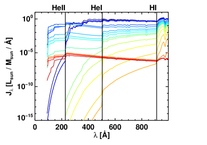
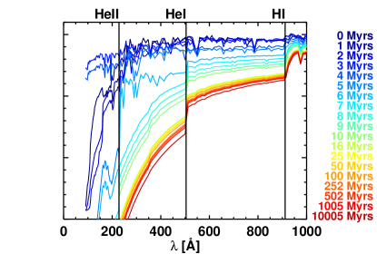
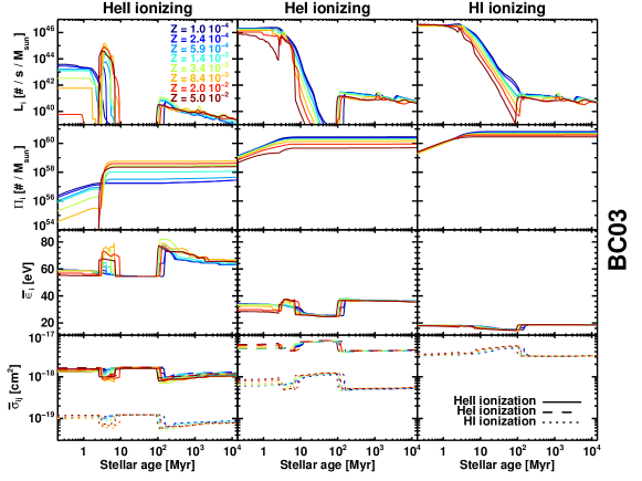
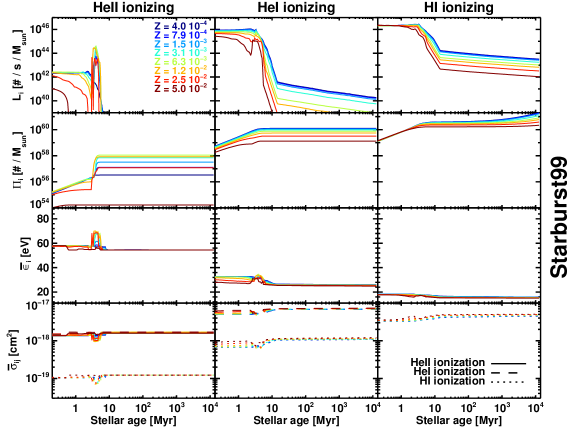
In the photon injection step in RAMSES-RT (§3.1), the task is to inject photons into each grid cell corresponding to the luminosities of stellar particles that reside in it. Here we describe how we derive these luminosities from stellar energy distribution (SED) models, along with the photoionization cross sections and energies for each photon group.

B.1 Stellar luminosities

Stellar particles in RAMSES represent stellar populations, so it makes sense to use SED models to infer their luminosities. RAMSES-RT can read SED tables at startup and derive from them stellar luminosities for photon injection, as well as photon group attributes that can be updated to reflect the average emission from the stellar particles populating the simulation.

We have hitherto used the SED model of Bruzual & Charlot (2003) (BC03), but it can be replaced with any other model, e.g. Starburst99 (Leitherer et al., 1999), as long as the file format is adjusted to match. The model should come in the form of spectra, $J_{\lambda}({\tau},Z)$, giving emitted energy in Solar units per Solar mass per wavelength per second, binned by stellar population age and metallicity. In Fig. 30 we show $J_{\lambda}$ from BC03 and Starburst99 at solar metallicity for various population ages.

Age and metallicity dependent population luminosity $L$, given in number of photons emitted per second into photon group $i$, is calculated from the SED model by

$$L_{i}({\tau},Z)=\int_{{\nu_{i\scriptscriptstyle 0}}}^{{\nu_{i\scriptscriptstyle 1}}}{J_{\nu}({\tau},Z)/h\nu\ d\nu},$$ (87)

where $J_{\nu}=c/\nu^{2}J_{\lambda(\nu)}$. The cumulative population luminosity is then

$$\Pi_{i}({\tau},Z)=\int_{0}^{{\tau}}{L_{i}(t,Z)\ dt}.$$ (88)

Since both the photon injection and the calculation of photon group attributes are done on the fly, $L_{i}({\tau},Z)$ and $\Pi_{i}({\tau},Z)$ must be evaluated as quickly as possible for given stellar particle ages and metallicities. Values of $L_{i}$ and $\Pi_{i}$ are therefore only calculated from the SED spectra via (87) and (88) at simulation startup, and tabulated with equally-spaced logarithmic bins of age and metallicity, so that they can be retrieved with minimum computational effort via linear interpolation, e.g. when injecting photons into cells via Eq. 17.

B.2 Photon group attributes

There are three sets of global attributes for each photon group. These are average photon energies $\bar{\epsilon}_{i}$, average photoionization cross sections ${\sigma}^{\rm{N}}_{ij}$ and energy weighted cross sections ${\sigma}^{\rm{E}}_{ij}$, that are defined in §2 (Eqs. 9-11). For an age and metallicity dependent reference spectrum $J_{\nu}({\tau},Z)$, these are

$$\bar{\epsilon}_{i}({\tau},Z)=\frac{\int_{{\nu_{i\scriptscriptstyle 0}}}^{{\nu_{i\scriptscriptstyle 1}}}{J_{\nu}\ d\nu}}{\int_{{\nu_{i\scriptscriptstyle 0}}}^{{\nu_{i\scriptscriptstyle 1}}}{J_{\nu}/h\nu\ d\nu}},$$ (89)

$${\sigma}^{\rm{N}}_{ij}({\tau},Z)=\frac{\int_{{\nu_{i\scriptscriptstyle 0}}}^{{\nu_{i\scriptscriptstyle 1}}}{\sigma_{\nu j}J_{\nu}/h\nu\ d\nu}}{\int_{{\nu_{i\scriptscriptstyle 0}}}^{{\nu_{i\scriptscriptstyle 1}}}{J_{\nu}/h\nu\ d\nu}},$$ (90)

$${\sigma}^{\rm{E}}_{ij}({\tau},Z)=\frac{\int_{{\nu_{i\scriptscriptstyle 0}}}^{{\nu_{i\scriptscriptstyle 1}}}{\sigma_{\nu j}J_{\nu}\ d\nu}}{\int_{{\nu_{i\scriptscriptstyle 0}}}^{{\nu_{i\scriptscriptstyle 1}}}{J_{\nu}\ d\nu}}.$$ (91)

Since there are three ionizeable species in the current implementation of RAMSES-RT, each photon group has three values of ${\sigma}^{\rm{N}}$ and three of ${\sigma}^{\rm{E}}$. These attributes can be set as run parameters to reflect some typical stellar spectra, e.g. a blackbody or a SED. It can also be left to RAMSES-RT to set them on the fly to reflect the in-simulation stellar populations, using the expressions (89)-(91), with the loaded SED spectra representing $J_{\nu}$ and the expressions from Verner et al. (1996) for $\sigma_{\nu j}$ (see Appendix E.4). Due to the averaged nature of the photon groups, we must however suffice to set the group attributes to reflect the average stellar emission in the simulation, weighted by the stellar luminosities . If this option is used, the photon group attributes are updated every $n$ coarse time-steps (where $n$ is an adjustable parameter) by polling all the stellar particles in the simulation and setting for each group $i$ and species $j$,

$$\bar{\epsilon}_{i}=\frac{\sum\limits^{\textrm{all stars}}_{\star}\bar{\epsilon}_{i}({\tau_{\star}},Z_{\star})\ m_{\star}\ L_{i}({\tau_{\star}},Z_{\star})}{\sum\limits^{\textrm{all stars}}_{\star}\ m_{\star}\ L_{i}({\tau_{\star}},Z_{\star})}.$$ (92)

$${\sigma}^{\rm{N}}_{ij}=\frac{\sum\limits^{\textrm{all stars}}_{\star}{\sigma}^{\rm{N}}_{ij}({\tau_{\star}},Z_{\star})\ m_{\star}\ L_{i}({\tau_{\star}},Z_{\star})}{\sum\limits^{\textrm{all stars}}_{\star}\ m_{\star}\ L_{i}({\tau_{\star}},Z_{\star})},$$ (93)

$${\sigma}^{\rm{E}}_{ij}=\frac{\sum\limits^{\textrm{all stars}}_{\star}{\sigma}^{\rm{E}}_{ij}({\tau_{\star}},Z_{\star})\ m_{\star}\ L_{i}({\tau_{\star}},Z_{\star})}{\sum\limits^{\textrm{all stars}}_{\star}\ m_{\star}\ L_{i}({\tau_{\star}},Z_{\star})}.$$ (94)

The values of each stellar particle’s $L_{i}({\tau_{\star}},Z_{\star})$, $\bar{\epsilon}_{ij}({\tau_{\star}},Z_{\star})$, ${\sigma}^{\rm{N}}_{ij}({\tau_{\star}},Z_{\star})$ and ${\sigma}^{\rm{E}}_{ij}({\tau_{\star}},Z_{\star})$ are interpolated from tables that are generated at startup via (87) and (89)-(91).

Although one is free to use many photon groups to resolve frequencies, it is practical to only use a handful, due to limitations in memory and computation. We typically use three photon groups in our simulations, representing ${\rm{H\textsc{i}}}$, ${\rm{He\textsc{i}}}$ and $\rm{He\textsc{ii}}$ ionizing photons, as indicated by vertical lines in the plots of Fig. 30. The stellar luminosities, instantaneous and accumulated, average cross sections and energies for those groups are plotted in Fig. 31 for BC03 (top) and Starburst99 (bottom), as calculated via (87)-(91). From the luminosity plots (top rows), it can be seen that the stellar populations emit predominantly for the first $\sim 3-6$ Myrs and the luminosity drastically goes down as the most massive stars in the population begin to expire.

Appendix C Non-equilibrium thermochemistry tests

To validate the non-equilibrium thermochemistry in RAMSES-RT we ran one-cell thermochemistry tests, that start at some initial state (temperature, ionization state, photon flux) and evolve over roughly a Hubble time. We are interested here in verifying that our implementation is correct and error free and also in comparing equilibrium vs. non-equilibrium cooling – e.g. Cen & Fang (2006) report that the methods can produce significantly different results. We compare against the equilibrium thermochemistry of RAMSES which has been modified to use the exact same heating, cooling and interaction rates as RAMSES-RT.

We test to see (i) whether the thermochemistry of RAMSES-RT is stable, i.e. if the stiffness of the equations results in any sudden divergence or ‘wiggles’ in the evolution of the gas, (ii) whether RAMSES-RT evolves the ionization fractions towards the correct states predicted by the equilibrium solver of RAMSES, and (iii) whether the RAMSES and RAMSES-RT evolve the temperature towards the same final value.

There are four tests: first we disable cooling and evolve only the ionization states of hydrogen and helium at different constant temperatures in a zero UV radiation field, and see if we reach equilibrium ionization states (predicted by RAMSES). Then we turn on a constant UV radiation field and again see if we reach equilibrium states. Then we turn on cooling, and for two sets (zero, nonzero radiation field) see if the temperature evolution is comparable to RAMSES equilibrium cooling from the same initial conditions.

C.1 Ionization convergence at constant temperature and zero ionizing photon flux

Figure 32: Ionization convergence test with constant $T$ and zero ionizing photon flux. Coloured lines show non-equilibrium evolution of the ionization fractions, given constant $T$ (right) and $n_{\rm{H}}$ (top). Black dashed lines show the corresponding equilibrium ionization fractions as calculated in RAMSES.

In the first test, cooling is turned off and we check for a range of densities, temperatures and initial ionization states whether we get a convergence of the ionized fractions towards their equilibrium states, as predicted by RAMSES, assuming zero flux of ionizing photons.

Fig. 32 shows the results. Each panel of $3\times 6$ plots in the figure represents an evolution given the constant temperature written to the right of the panel, and shows how the ionized fractions, $x_{\rm{H\scriptscriptstyle II}}$, $x_{\rm{He\scriptscriptstyle II}}$ and $x_{\rm{He\scriptscriptstyle III}}$, evolve from different (color-coded) starting states $x_{i}=x_{\rm{H\scriptscriptstyle II}}=x_{\rm{He\scriptscriptstyle III}}$ (the HeII fraction always starts at zero). A black dashed line in each plot shows the equilibrium ionization fraction for the given temperature and species (which is gas density independent in the case of zero ionizing flux). Each column of plots represents a (non-evolving) hydrogen number density.

The non-equilibrium ionization fractions always evolve towards the equilibrium ones, at a rate which depends on gas density, as expected. It can even take longer than the age of the Universe to reach equilibrium for the most diffuse gas ($n_{\rm{H}}\la 10^{-6}\ {\rm{cm}}^{-3}$), which indeed is a significant difference from the equilibrium assumption. If we zoom in around the equilibrium states we find a difference between the calculated equilibrium state and the evolved one which is typically around one in ten-thousand - this simply corresponds to the allowed error in the iterative equilibrium calculation, and can be decreased at will by reducing this error margin.

C.2 Ionization convergence at constant temperature and nonzero ionizing photon flux

Figure 33: Ionization convergence test with constant temperature and an ionizing photon flux of $10^{5}\;\;{\rm{s}}^{-1}\,{\rm{cm}}^{-2}$.

Figure 34: Temperature convergence with zero ionizing flux. Color coded lines show different initial states of $x_{\rm{H\scriptscriptstyle II}}$ and $x_{\rm{He\scriptscriptstyle III}}$, as indicated by the color legend at bottom right. Black dashed curves show the equilibrium evolution from RAMSES.

Figure 35: Temperature convergence with an ionizing photon flux of $10^{5}\;\;{\rm{s}}^{-1}\,{\rm{cm}}^{-2}$.

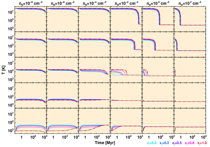
This is the same as the previous test, except now we apply a constant flux of $10^{5}$ ionizing photons ${\rm{s}}^{-1}\,{\rm{cm}}^{-2}$ through the cell, assuming the spectrum of a blackbody at $10^{5}$ K.

Fig. 33 shows the results. The black dashed lines in each plot show the equilibrium state which now is density dependent - the denser the gas the harder it is for the radiation field to battle against recombinations. Again the non-equilibrium ionized state always evolves towards the equilbrium one at a gas density dependent rate, though note that here it takes a maximum of $\sim 10$ Myr, which is much shorter than it can take in the zero photon flux case.

C.3 Temperature convergence with zero ionizing photon flux

Now cooling is turned on, and we compare the RAMSES-RT non-equilibrium temperature evolution with that of equilibrium RAMSES (though keep in mind it has been adjusted to contain the exact same cooling rates as RAMSES-RT). Each of the 5 rows in fig. 34 shows cooling for a range of decreasing initial temperatures, from top to bottom. The color-codings (initial ionization states) and columns (hydrogen number densities) are the same as before. The solid colored lines show non-equilibrium cooling in RAMSES-RT and the black dashed lines represent equilibrium cooling in RAMSES starting from the same temperature.

Clearly the temperature evolution is quite similar between equilibrium/non-equilibrium cooling, especially if the initial ionization fraction is ’correct’, i.e. if it matches the equilibrium one at the initial temperature.

The final temperature reached in the non-equilibrium case is usually a bit lower than in the equilibrium case. This is independent of gas density and initial temperature (as long as the initial temperature allows for cooling to happen). The reason for this is that the non-equilibrium ionization evolution lags behind the instantaneous equilibrium one, so there is always a somewhat larger reservoir of electrons in the non-equilibrium case. Electrons are the primary cooling agents, and complete electron depletion completely stops cooling, so it makes sense that if the electrons deplete more slowly, cooling is more effective and can bring the gas to a lower final temperature.

C.4 Temperature convergence with nonzero ionizing photon flux

This is the same as the previous test, except now we apply a constant flux of $10^{5}$ ionizing photons ${\rm{s}}^{-1}\,{\rm{cm}}^{-2}$, assuming the spectrum of a blackbody at $10^{5}$ K. The results are shown in Fig. 35. Things are much the same as before, except that the non-equilibrium temperature seems to converge to a value which is much closer to the the equilibrium one - because of the ionizing flux there is always a reservoir of electrons both in the equilibrium and non-equilibrium evolution, which makes for a much closer match in the final temperature.

Although the final temperature reached is identical between the two methods, the evolution towards that final temperature can be quite different, depending on the initial ionization states.

A zoom-in on one of the plots is shown in Fig. 36, and reveals that there is very little difference between the final temperatures reached. The little difference there is results from interpolation from cooling-rate tables in RAMSES equilibrium cooling and it can be decreased further by increasing the size of these tables.

C.5 Thermochemistry tests conclusions

The main conclusions of the one-cell thermochemistry tests are:

• We always eventually reach the equilibrium ionization state with the non-equilibrium method…

• …but this can take a very long time to happen for diffuse gas, even more than a Hubble time.

• Non-equilibrium temperature evolution of the gas is quite dependent on the initial ionization fraction of the gas at intermediate temperatures and low densities…

• …but in the end we reach the same or at least a very similar temperature as in the equilibrium case.

• The convergence of the non-equilibrium solver towards the results of the equilibrium solver of RAMSES, given the same cooling rate expressions, suggests that our thermochemistry solver is robust and correct.

Figure 36: Close-up of temperature convergence, for the UV inclusive test with initial temperature $T\approx 10^{5}$ K and $n_{\rm{H}}=10^{-2}$ ${\rm{cm}}^{-3}$

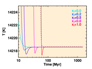
Appendix D On multi-stepping in the AMR level hierarchy

As discussed in §5.2, solving hydrodynamics over an AMR grid with a multi-stepping approach always leaves ill-defined states at inter-level boundaries between the start and finish of the coarse level timestep. This imposes severe constraints on how the RT can be coupled to the hydrodynamics, and essentially means that RT cannot be sub-cycled within multi-stepping hydrodynamics. Here we will clarify this point in detail.

Hydrodynamic advection across the boundaries of a cell is performed in an operator-split fashion, such that the advection is solved separately across a discretized timestep for each boundary. In order for the solver to be consistent, i.e. for the result at the end of the timestep to be independent of the order in which the boundaries are accounted for, the solver must work from the same initial cell state ${\mathcal{U}}$ for all the inter-cell updates. Thus, a copy is first made of the original cell states involved, i.e.

$${\mathcal{U}}\rightarrow{\widetilde{\mathcal{U}}},$$ (95)

where we can term ${\mathcal{U}}$ the source state and ${\widetilde{\mathcal{U}}}$ the destination state. Using ${\mathcal{U}}$ as source terms for the intercell fluxes, the advection can be solved with some computational method (e.g. Godunov solver for the hydrodynamics in RAMSES and an HLL/GLF flux function for the RT advection in RAMSES-RT), which performs the update on ${\widetilde{\mathcal{U}}}$. To take a concrete example, each RT advection update, Eq. 22, uses ${\widetilde{\mathcal{U}}}$ for the update (the LHS term and the first RHS term), but the intercell fluxes are derived from ${\mathcal{U}}$, i.e. ${\mathcal{F}}({\mathcal{U}})$. Once all the updates (6 per cell) have been collected, the cell update is made final by:

$${\widetilde{\mathcal{U}}}\rightarrow{\mathcal{U}}.$$ (96)

In the $\tt{amr\_step(\ell)}$ hierarchy in RAMSES, such copies are made of all $\ell$ cells before the AMR recursion, and the update is made final after the recursion has returned and the $\tt{hydro\_solver}$ has been called at the current level, i.e. advection has been performed over the timestep over the current level and all finer levels.

This allows cell states to be updated not only at the current level, but also (twice) in all neighbouring cells at the next coarser level. The coarser level update is only partial though, because it only reflects the intercell fluxes across inter-level boundaries, and fluxes across other boundaries (same level or next coarser level) will only be accounted for when the coarser level time-step is advanced. Until then, these coarser level neighbour cells have two gas states, ${\mathcal{U}}$ and ${\widetilde{\mathcal{U}}}$. This is shown schematically in Fig. 37.

Figure 37: Level $\ell$ gas state updates via intercell fluxes also perform partial gas updates in neighbouring cells at level $\ell-1$. The example shown corresponds to the hierarchy from Fig. 5. Steps 3 and 4 at the finest level also include partial updates of neighbouring $\ell_{\rm{max}}-1$ cells, but these neighbour cell states are not fully updated until all the intercell fluxes are taken into account, which is in step 5 from Fig. 5.

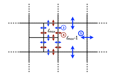
If RT subcycling is to be done at each AMR fine-level step, over the whole grid, the question is, which cell state do we use for the thermochemistry, i.e. the interaction between photons and gas, in those inter-level boundary cells?

Choosing one but not the other leads to an obvious and severe inconsistency between the source and destination states. If the thermochemistry does the update on ${\widetilde{\mathcal{U}}}$, then a gas element which is transported from one cell to a neighbour during the following hydro transport is not thermochemically evolved over the time-step, because it originates from ${\mathcal{U}}$. If instead the update is done on ${\mathcal{U}}$, a gas element which stays still in any cell over the following hydro transport step is not thermochemically evolved over the time-step. One might then just update both states via thermochemistry, i.e. apply it on each cell twice. This does not really make sense for these inter-level intercell boundary cells that have ${\mathcal{U}}\neq{\widetilde{\mathcal{U}}}$, as ${\widetilde{\mathcal{U}}}$ doesn’t represent a true state but is rather an intermediate and temporary quantity that exists between well-defined times. Also, it would be really non-trivial to implement: applying thermochemistry on each of the states also implies transporting the photons through two different states in each cell, which creates alternative time-lines for the radiative transfer!

Thus, subcycling RT within multi-stepping hydrodynamics in a conservative way is not possible (or at least non-trivial), which has led us to disallow RT subcycling within the hydro timestep in our implementation.

Appendix E Interaction rate coefficients adopted in RamsesRT

Here we collect the rate coefficients used in RAMSES-RT for hydrogen and helium interactions, which are fitted functions taken from various sources. These are, in order of appearance, collisional ionization rates, recombination rates, cooling rates (collisional ionization, recombination, collisional excitation, bremsstrahlung, Compton and dielectric recombination), and photoionization cross sections.

E.1 Collisional ionization rate coefficients

Those are in units of [$\rm{cm}^{3}\,\rm{s}^{-1}$] and are taken from Cen (1992), with temperature everywhere assumed in Kelvin:

$$\beta_{{\rm{H\textsc{i}}}}(T) =5.85\times 10^{-11}\ \sqrt{T}\ \left(1+\sqrt{\frac{T}{10^{5}}}\right)^{-1}\ e^{-157\ 809.1/T}$$

$$\beta_{{\rm{He\textsc{i}}}}(T) =2.38\times 10^{-11}\ \sqrt{T}\ \left(1+\sqrt{\frac{T}{10^{5}}}\right)^{-1}\ e^{-285\ 335.4/T}$$

$$\beta_{\rm{He\textsc{ii}}}(T) =5.68\times 10^{-12}\ \sqrt{T}\ \left(1+\sqrt{\frac{T}{10^{5}}}\right)^{-1}\ e^{-631\ 515/T}$$

E.2 Recombination rate coefficients

These are all taken from Hui & Gnedin (1997). For readability, we use the following unitless functions:

$$\lambda_{{\rm{H\textsc{i}}}}(T) =\frac{315\ 614\ K}{T}$$

$$\lambda_{{\rm{He\textsc{i}}}}(T) =\frac{570\ 670\ K}{T}$$

$$\lambda_{\rm{He\textsc{ii}}}(T) =\frac{1\ 263\ 030\ K}{T}$$

The coefficients are as follows, all in units of [$\rm{cm}^{3}\,\rm{s}^{-1}$]:

$$\alpha^{\rm{A}}_{\rm{H\textsc{ii}}}(T) =1.269\times 10^{-13}\ \frac{\lambda^{1.503}_{{\rm{H\textsc{i}}}}}{[1+(\lambda_{{\rm{H\textsc{i}}}}/0.522)^{0.47}]^{1.923}}$$

$$\alpha^{\rm{A}}_{\rm{He\textsc{ii}}}(T) =3\times 10^{-14}\ \lambda^{0.654}_{{\rm{He\textsc{i}}}}$$

$$\alpha^{\rm{A}}_{\rm{He\textsc{iii}}}(T) =2.538\times 10^{-13}\ \frac{\lambda^{1.503}_{\rm{He\textsc{ii}}}}{[1+(\lambda_{\rm{He\textsc{ii}}}/0.522)^{0.47}]^{1.923}}$$

$$\alpha^{\rm{B}}_{\rm{H\textsc{ii}}}(T) =2.753\times 10^{-14}\ \frac{\lambda^{1.5}_{{\rm{H\textsc{i}}}}}{[1+(\lambda_{{\rm{H\textsc{i}}}}/2.74)^{0.407}]^{2.242}}$$

$$\alpha^{\rm{B}}_{\rm{He\textsc{ii}}}(T) =1.26\times 10^{-14}\ \lambda^{0.75}_{{\rm{He\textsc{i}}}}$$

$$\alpha^{\rm{B}}_{\rm{He\textsc{iii}}}(T) =5.506\times 10^{-14}\ \frac{\lambda^{1.5}_{\rm{He\textsc{ii}}}}{[1+(\lambda_{\rm{He\textsc{ii}}}/2.74)^{0.407}]^{2.242}}$$

Table 2: Photoionization cross section parameters – see Eq. 97

Ion species	$\epsilon_{0}$ [eV]	$\sigma_{0}$ [$\rm{cm}^{2}$]	$P$	$y_{a}$	$y_{w}$	$y_{0}$	$y_{1}$
Hi	$0.4298$	$5.475\ 10^{-14}$	$2.963$	$32.88$	$0$	$0$	$0$
Hei	$0.1361$	$9.492\ 10^{-16}$	$3.188$	$1.469$	$2.039$	$0.4434$	$2.136$
Heii	$1.720$	$1.369\ 10^{-14}$	$2.963$	$32.88$	$0$	$0$	$0$

E.3 Cooling rate coefficients

The temperature used in these coefficients is assumed everywhere in Kelvin. Collisional ionization cooling rate coefficients [$\rm{erg}\,\rm{cm}^{3}\,\rm{s}^{-1}$] (Cen, 1992):

$$\zeta_{{\rm{H\textsc{i}}}}(T) =1.27\times 10^{-21}\ \sqrt{T}\ \left(1+\sqrt{\frac{T}{10^{5}}}\right)^{-1}\ e^{-157\ 809.1/T}$$

$$\zeta_{{\rm{He\textsc{i}}}}(T) =9.38\times 10^{-22}\ \sqrt{T}\ \left(1+\sqrt{\frac{T}{10^{5}}}\right)^{-1}\ e^{-285\ 335.4/T}$$

$$\zeta_{\rm{He\textsc{ii}}}(T) =4.95\times 10^{-22}\ \sqrt{T}\ \left(1+\sqrt{\frac{T}{10^{5}}}\right)^{-1}\ e^{-631\ 515/T}$$

Case A and B recombination cooling rate coefficients [$\rm{erg}\,\rm{cm}^{3}\,\rm{s}^{-1}$] (Hui & Gnedin, 1997):

$$\eta^{A}_{\rm{H\textsc{ii}}}(T) =1.778\times 10^{-29}\ T\ \frac{\lambda^{1.965}_{{\rm{H\textsc{i}}}}}{[1+(\lambda_{{\rm{H\textsc{i}}}}/0.541)^{0.502}]^{2.697}}$$

$$\eta^{A}_{\rm{He\textsc{ii}}}(T) =k_{\rm{B}}\ T\alpha^{\rm{A}}_{\rm{He\textsc{ii}}}\ =\ k_{\rm{B}}\ T\ 3\times 10^{-14}\ \lambda^{0.654}_{{\rm{He\textsc{i}}}}$$

$$\eta^{A}_{\rm{He\textsc{iii}}}(T) =8\times 1.778\times 10^{-29}\ T\ \frac{\lambda^{1.965}_{\rm{He\textsc{ii}}}}{[1+(\lambda_{\rm{He\textsc{ii}}}/0.541)^{0.502}]^{2.697}}$$

$$\eta^{B}_{\rm{H\textsc{ii}}}(T) =3.435\times 10^{-30}\ T\ \frac{\lambda^{1.97}_{{\rm{H\textsc{i}}}}}{[1+(\lambda_{{\rm{H\textsc{i}}}}/2.25)^{0.376}]^{3.72}}$$

$$\eta^{B}_{\rm{He\textsc{ii}}}(T) =k_{\rm{B}}\ T\alpha^{\rm{B}}_{\rm{He\textsc{ii}}}\ =\ k_{\rm{B}}\ T\ 1.26\times 10^{-14}\ \lambda^{0.75}_{{\rm{He\textsc{i}}}}$$

$$\eta^{B}_{\rm{He\textsc{iii}}}(T) =8\times 3.435\times 10^{-30}\ T\ \frac{\lambda^{1.97}_{\rm{He\textsc{ii}}}}{[1+(\lambda_{\rm{He\textsc{ii}}}/2.25)^{0.376}]^{3.72}}$$

Collisional excitation cooling rate coefficients [$\rm{erg}\,\rm{cm}^{3}\,\rm{s}^{-1}$] (Cen, 1992):

$$\psi_{{\rm{H\textsc{i}}}}(T) =7.5\times 10^{-19}\ \left(1+\sqrt{\frac{T}{10^{5}}}\right)^{-1}\ e^{-118\ 348/T}$$

$$\psi_{\rm{He\textsc{ii}}}(T) =5.54\times 10^{-17}\ T^{-0.397}\left(1+\sqrt{\frac{T}{10^{5}}}\right)^{-1}e^{-473\ 638/T}$$

Bremsstrahlung cooling rate coefficients [$\rm{erg}\,\rm{cm}^{3}\,\rm{s}^{-1}$] (Osterbrock & Ferland, 2006):

$$\theta_{\rm{H\textsc{ii}}}(T) =1.42\times 10^{-27}\sqrt{T}$$

$$\theta_{\rm{He\textsc{ii}}}(T) =1.42\times 10^{-27}\sqrt{T}$$

$$\theta_{\rm{He\textsc{iii}}}(T) =4\times 1.42\times 10^{-27}\sqrt{T}$$

Compton cooling/heating rate coefficient [$\rm{erg}\,\rm{s}^{-1}$] (Haiman, Thoul & Loeb, 1996), with $a$ the cosmological expansion factor and $T_{\gamma}\equiv 2.727/a$ K the temperature of the cosmic background radiation.:

$$\varpi(T,a) =1.017\times 10^{-37}\ \left(\frac{2.727}{a}\right)^{4}\ \left(T-\frac{2.727}{a}\right)$$

Dielectronic recombination cooling rate coefficient [$\rm{erg}\,\rm{cm}^{3}\,\rm{s}^{-1}$] (Black, 1981):

$$\omega_{\rm{He\textsc{ii}}}(T) =1.24\times 10^{-13}T^{-1.5}e^{-470\ 000/T}\left(1+0.3e^{-94\ 000/T}\right)$$

E.4 Cross sections

Table 3: Photoionization energies and corresponding frequencies

Ion species	$\epsilon_{ion}$	$\nu_{ion}$
Hi	$\epsilon_{{\rm{H\textsc{i}}}}=13.60$   eV	$\nu_{{\rm{H\textsc{i}}}}=3.288\ 10^{15}$    $\rm{s}^{-1}$
Hei	$\epsilon_{{\rm{He\textsc{i}}}}=24.59$   eV	$\nu_{{\rm{He\textsc{i}}}}=5.946\ 10^{15}$    $\rm{s}^{-1}$
Heii	$\epsilon_{\rm{He\textsc{ii}}}=54.42$   eV	$\nu_{\rm{He\textsc{ii}}}=1.316\ 10^{16}$    $\rm{s}^{-1}$

Expressions for frequency dependent photoionization ${\rm{H\textsc{i}}}-$, $\rm{He\textsc{ii}}-$ and $\rm{He\textsc{iii}}-$ cross sections are used in RAMSES-RT to derive photon group attributes from stellar populations (Appendix B). These expressions are taken from Verner et al. (1996) (via Hui & Gnedin, 1997) and are given in [$\rm{cm}^{2}$] as a function of photon energy $\epsilon$ by

$$\sigma(\epsilon)=\sigma_{0}\left[(x-1)^{2}+y_{w}^{2}\right]\frac{y^{0.5P-5.5}}{(1+\sqrt{y/y_{a}})^{P}} \mbox{, if $\epsilon\geq\epsilon_{ion}$},$$ (97)

(and $0\ \rm{cm}^{2}$ otherwise), where

$$x\equiv\frac{\epsilon}{\epsilon_{0}}-y_{0},$$

and

$$y\equiv\sqrt{x^{2}+y_{1}^{2}},$$

and the fitting parameters $\sigma_{0}$, $\epsilon_{0}$, $y_{w}$, $P$, $y_{a}$, $y_{0}$, and $y_{1}$ are given in Table 2. The ionization energies $\epsilon_{ion}$ and corresponding frequencies $\nu_{ion}$ are given in Table 3.

References

- Abel, Norman & Madau (1999) Abel T., Norman M. L., Madau P., 1999, ApJ, 523, 66
- Abel & Wandelt (2002) Abel T., Wandelt B. D., 2002, MNRAS, 330, L53
- Agertz et al. (2007) Agertz O. et al., 2007, Monthly Notices of the Royal Astronomical Society, 380, 963
- Altay, Croft & Pelupessy (2008) Altay G., Croft R. A. C., Pelupessy I., 2008, MNRAS, 386, 1931
- Alvarez, Bromm & Shapiro (2006) Alvarez M. A., Bromm V., Shapiro P. R., 2006, ApJ, 639, 621
- Anninos et al. (1997) Anninos P., Zhang Y., Abel T., Norman M. L., 1997, New Astronomy, 2, 209
- Aubert & Teyssier (2008) Aubert D., Teyssier R., 2008, MNRAS, 387, 295
- Aubert & Teyssier (2010) Aubert D., Teyssier R., 2010, ApJ, 724, 244
- Baek et al. (2009) Baek S., Di Matteo P., Semelin B., Combes F., Revaz Y., 2009, A&A, 495, 389
- Baek et al. (2010) Baek S., Semelin B., Di Matteo P., Revaz Y., Combes F., 2010, A&A, 523, 4
- Black (1981) Black J. H., 1981, MNRAS, 197, 553
- Bruzual & Charlot (2003) Bruzual G., Charlot S., 2003, MNRAS, 344, 1000
- Cantalupo & Porciani (2011) Cantalupo S., Porciani C., 2011, Monthly Notices of the Royal Astronomical Society, 411, 1678
- Cantalupo et al. (2005) Cantalupo S., Porciani C., Lilly S. J., Miniati F., 2005, ApJ, 628, 61
- Cen (1992) Cen R., 1992, ApJS, 78, 341
- Cen (2002) Cen R., 2002, AJS, 141, 211
- Cen & Fang (2006) Cen R., Fang T., 2006, ApJ, 650, 573
- Ciardi et al. (2001) Ciardi B., Ferrara A., Marri S., Raimondo G., 2001, MNRAS, 324, 381
- Ciardi, Stoehr & White (2003) Ciardi B., Stoehr F., White S. D. M., 2003, Monthly Notice of the Royal Astronomical Society, 343, 1101
- Commerçon et al. (2011) Commerçon B., Teyssier R., Audit E., Hennebelle P., Chabrier G., 2011, A&A, 529, 35
- Croft & Altay (2008) Croft R. A. C., Altay G., 2008, MNRAS, 388, 1501
- Dijkstra & Loeb (2009) Dijkstra M., Loeb A., 2009, MNRAS, 396, 377
- Dubroca & Feugeas (1999) Dubroca B., Feugeas J., 1999, Comptes Rendus de l’Académie des Sciences - Series I - Mathematics, 329, 915
- Finlator, Dave & Ozel (2011) Finlator K., Dave R., Ozel F., 2011, ApJ, 743, 169
- Finlator, Özel & Davé (2009) Finlator K., Özel F., Davé R., 2009, MNRAS, 393, 1090
- Gnedin (2000) Gnedin N. Y., 2000, ApJ, 535, 530
- Gnedin & Abel (2001) Gnedin N. Y., Abel T., 2001, New Astronomy, 6, 437
- Gnedin & Ostriker (1997) Gnedin N. Y., Ostriker J. P., 1997, Astrophysical Journal v.486, 486, 581
- González, Audit & Huynh (2007) González M., Audit E., Huynh P., 2007, A&A, 464, 429
- Haiman, Thoul & Loeb (1996) Haiman Z., Thoul A. A., Loeb A., 1996, Astrophysical Journal v.464, 464, 523
- Harten, Lax & Leer (1983) Harten A., Lax P. D., Leer B. v., 1983, SIAM review, 25, 35
- Hasegawa & Semelin (2013) Hasegawa K., Semelin B., 2013, Monthly Notices of the Royal Astronomical Society, 428, 154
- Hopkins et al. (2012) Hopkins P. F., Kereš D., Murray N., Quataert E., Hernquist L., 2012, Monthly Notices of the Royal Astronomical Society, 427, 968
- Hopkins, Quataert & Murray (2011) Hopkins P. F., Quataert E., Murray N., 2011, MNRAS, 417, 950
- Hui & Gnedin (1997) Hui L., Gnedin N. Y., 1997, MNRAS, 292, 27
- Iliev et al. (2006a) Iliev I. T. et al., 2006a, MNRAS, 371, 1057
- Iliev et al. (2006b) Iliev I. T., Mellema G., Pen U.-L., Merz H., Shapiro P. R., Alvarez M. A., 2006b, MNRAS, 369, 1625
- Iliev et al. (2009) Iliev I. T. et al., 2009, MNRAS, 400, 1283
- Kohler, Gnedin & Hamilton (2007) Kohler K., Gnedin N. Y., Hamilton A. J. S., 2007, ApJ, 657, 15
- Krumholz, Klein & McKee (2012) Krumholz M. R., Klein R. I., McKee C. F., 2012, ApJ, 754, 71
- Krumholz et al. (2007) Krumholz M. R., Klein R. I., McKee C. F., Bolstad J., 2007, ApJ, 667, 626
- Laursen & Sommer-Larsen (2007) Laursen P., Sommer-Larsen J., 2007, ApJ, 657, L69
- Leitherer et al. (1999) Leitherer C. et al., 1999, AJS, 123, 3
- Levermore (1984) Levermore C. D., 1984, Journal of Quantitative Spectroscopy and Radiative Transfer, 31, 149
- Martel & Shapiro (1998) Martel H., Shapiro P. R., 1998, MNRAS, 297, 467
- Maselli, Ciardi & Kanekar (2009) Maselli A., Ciardi B., Kanekar A., 2009, MNRAS, 393, 171
- Maselli, Ferrara & Ciardi (2003) Maselli A., Ferrara A., Ciardi B., 2003, MNRAS, 345, 379
- Mellema et al. (2006) Mellema G., Iliev I. T., Alvarez M. A., Shapiro P. R., 2006, New Astronomy, 11, 374
- Mihalas & Mihalas (1984) Mihalas D., Mihalas B. W., 1984, New York
- Miralda-Escudé, Haehnelt & Rees (2000) Miralda-Escudé J., Haehnelt M., Rees M. J., 2000, ApJ, 530, 1
- Nakamoto, Umemura & Susa (2001) Nakamoto T., Umemura M., Susa H., 2001, MNRAS, 321, 593
- Ocvirk & Aubert (2011) Ocvirk P., Aubert D., 2011, MNRAS, 417, L93
- Oppenheimer & Schaye (2013) Oppenheimer B. D., Schaye J., 2013, arXiv, 1303, 19
- Osterbrock & Ferland (2006) Osterbrock D. E., Ferland G. J., 2006, Astrophysics of gaseous nebulae and active galactic nuclei
- Pawlik, Milosavljević & Bromm (2013) Pawlik A. H., Milosavljević M., Bromm V., 2013, ApJ, 767, 59
- Pawlik & Schaye (2008) Pawlik A. H., Schaye J., 2008, MNRAS, 389, 651
- Pawlik & Schaye (2009) Pawlik A. H., Schaye J., 2009, MNRAS, 396, L46
- Pawlik & Schaye (2011) Pawlik A. H., Schaye J., 2011, Monthly Notices of the Royal Astronomical Society, 412, 1943
- Petkova & Springel (2009) Petkova M., Springel V., 2009, Monthly Notices of the Royal Astronomical Society, 396, 1383
- Petkova & Springel (2011a) Petkova M., Springel V., 2011a, Monthly Notices of the Royal Astronomical Society, 415, 3731
- Petkova & Springel (2011b) Petkova M., Springel V., 2011b, Monthly Notices of the Royal Astronomical Society, 412, 935
- Pierleoni, Maselli & Ciardi (2009) Pierleoni M., Maselli A., Ciardi B., 2009, MNRAS, 393, 872
- Powell, Slyz & Devriendt (2011) Powell L. C., Slyz A., Devriendt J., 2011, MNRAS, 414, 3671
- Razoumov & Cardall (2005) Razoumov A. O., Cardall C. Y., 2005, MNRAS, 362, 1413
- Reynolds et al. (2009) Reynolds D. R., Hayes J. C., Paschos P., Norman M. L., 2009, Journal of Computational Physics, 228, 6833
- Ricotti, Gnedin & Shull (2002) Ricotti M., Gnedin N. Y., Shull J. M., 2002, ApJ, 575, 33
- Rijkhorst et al. (2006) Rijkhorst E.-J., Plewa T., Dubey A., Mellema G., 2006, A&A, 452, 907
- Rosdahl & Blaizot (2012) Rosdahl J., Blaizot J., 2012, MNRAS, 2837
- Scannapieco et al. (2012) Scannapieco C. et al., 2012, Monthly Notices of the Royal Astronomical Society, 423, 1726
- Shapiro et al. (2006) Shapiro P. R., Iliev I. T., Alvarez M. A., Scannapieco E., 2006, ApJ, 648, 922
- Shin, Trac & Cen (2008) Shin M. S., Trac H., Cen R., 2008, ApJ, 681, 756
- Sokasian et al. (2004) Sokasian A., Yoshida N., Abel T., Hernquist L., Springel V., 2004, MNRAS, 350, 47
- Sun (1996) Sun P., 1996, Journal of Computational Physics, 127, 152
- Susa (2006) Susa H., 2006, Publications of the Astronomical Society of Japan, 58, 445
- Tasker et al. (2008) Tasker E. J., Brunino R., Mitchell N. L., Michielsen D., Hopton S., Pearce F. R., Bryan G. L., Theuns T., 2008, Monthly Notices of the Royal Astronomical Society, 390, 1267
- Teyssier (2002) Teyssier R., 2002, A&A, 385, 337
- Toro (1999) Toro E. F., 1999, Riemann Solvers and Numerical Methods for Fluid Dynamics: A Practical Introduction. Berlin
- Trac & Pen (2004) Trac H., Pen U.-L., 2004, New Astronomy, 9, 443
- Vaytet, Audit & Dubroca (2010) Vaytet N., Audit E., Dubroca B., 2010, Numerical Modeling of Space Plasma Flows, 429, 160
- Verhamme, Schaerer & Maselli (2006) Verhamme A., Schaerer D., Maselli A., 2006, A&A, 460, 397
- Verner et al. (1996) Verner D. A., Ferland G. J., Korista K. T., Yakovlev D. G., 1996, Astrophysical Journal v.465, 465, 487
- Wadsley, Veeravalli & Couchman (2008) Wadsley J. W., Veeravalli G., Couchman H. M. P., 2008, Monthly Notices of the Royal Astronomical Society, 387, 427
- Whalen & Norman (2006) Whalen D., Norman M. L., 2006, AJS, 162, 281
- Wise & Abel (2008) Wise J. H., Abel T., 2008, ApJ, 685, 40
- Wise & Abel (2011) Wise J. H., Abel T., 2011, MNRAS, 414, 3458
- Yajima et al. (2012) Yajima H., Li Y., Zhu Q., Abel T., 2012, Monthly Notices of the Royal Astronomical Society, 424, 884
- Zahn et al. (2007) Zahn O., Lidz A., McQuinn M., Dutta S., Hernquist L., Zaldarriaga M., Furlanetto S. R., 2007, ApJ, 654, 12